1

Contents of Verilog Reference Guide

Contents of Verilog Reference Guide_____________________________________1

Always Procedural Block ______________________________________________3

Arithmetic Operators__________________________________________________5

Array______________________________________________________________7

Bit-Select __________________________________________________________9

Bit-wise Operators __________________________________________________10

Block Statement ____________________________________________________12

Blocking Assignment ________________________________________________14

Case Statement ____________________________________________________15

Comment _________________________________________________________17

Concatenation _____________________________________________________19

Conditional Operator ________________________________________________20

Continuous Assignment ______________________________________________21

Data Types ________________________________________________________23

Delays ___________________________________________________________24

Disable Statement __________________________________________________27

Equality Operators __________________________________________________28

Events ___________________________________________________________30

Expressions _______________________________________________________33

For Loop__________________________________________________________35

Forever Loop ______________________________________________________37

Function __________________________________________________________38

Gates ____________________________________________________________40

Identifier __________________________________________________________42

If Statement _______________________________________________________43

Initial Procedural Block_______________________________________________45

Integer Data Type___________________________________________________46

Integer Numbers____________________________________________________47

Logic Strength _____________________________________________________49

Logic Values_______________________________________________________50

Logical Operators ___________________________________________________51

Module Definition ___________________________________________________52

Module Instances ___________________________________________________54

2

Module Ports ______________________________________________________57

Net Data Types_____________________________________________________58

Non-Blocking Assignment_____________________________________________60

Number Representation ______________________________________________61

Operators _________________________________________________________62

Parameters________________________________________________________63

Part-Select ________________________________________________________65

Port Connections ___________________________________________________66

Primitives _________________________________________________________68

Primitive Instances __________________________________________________71

Procedural Assignments______________________________________________73

Procedural Blocks___________________________________________________75

Real Data Type_____________________________________________________77

Real Numbers______________________________________________________78

Reduction Operators ________________________________________________79

Register Data Types_________________________________________________81

Relational Operators_________________________________________________82

Repeat Loop_______________________________________________________83

Reserved Keywords _________________________________________________85

Shift Operators _____________________________________________________86

String Data Type____________________________________________________87

System Tasks and Functions __________________________________________88

Task _____________________________________________________________92

Time Data Type ____________________________________________________95

User Defined Primitive (UDP)__________________________________________96

Vector ____________________________________________________________99

Wait Statement____________________________________________________100

While Loop _______________________________________________________101

3

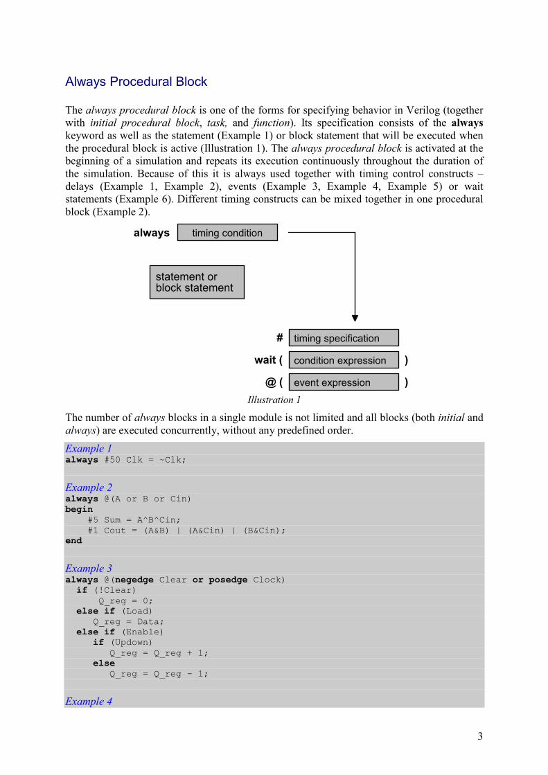
Always Procedural Block

The always procedural block is one of the forms for specifying behavior in Verilog (together with initial procedural block, task, and function). Its specification consists of the always keyword as well as the statement (Example 1) or block statement that will be executed when the procedural block is active (Illustration 1). The always procedural block is activated at the beginning of a simulation and repeats its execution continuously throughout the duration of the simulation. Because of this it is always used together with timing control constructs – delays (Example 1, Example 2), events (Example 3, Example 4, Example 5) or wait statements (Example 6). Different timing constructs can be mixed together in one procedural block (Example 2).

always

#

wait (

@ (

)

)

timing condition

event expression

condition expression

timing specification

statement orblock statement

Illustration 1

The number of always blocks in a single module is not limited and all blocks (both initial and always) are executed concurrently, without any predefined order.

Example 1 always #50 Clk = ~Clk;

Example 2 always @(A or B or Cin) begin #5 Sum = A^B^Cin; #1 Cout = (A&B) | (A&Cin) | (B&Cin); end

Example 3 always @(negedge Clear or posedge Clock) if (!Clear) Q_reg = 0; else if (Load) Q_reg = Data; else if (Enable) if (Updown) Q_reg = Q_reg + 1; else Q_reg = Q_reg - 1;

Example 4

4

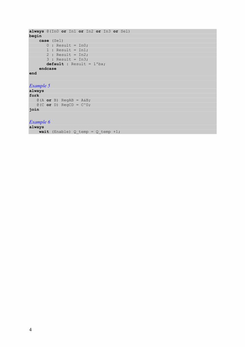
always @(In0 or In1 or In2 or In3 or Sel) begin case (Sel) 0 : Result = In0; 1 : Result = In1; 2 : Result = In2; 3 : Result = In3; default : Result = 1'bx; endcase end

Example 5 always

fork @(A or B) RegAB = A&B; @(C or D) RegCD = C^D; join

Example 6 always

wait (Enable) Q_temp = Q_temp +1;

5

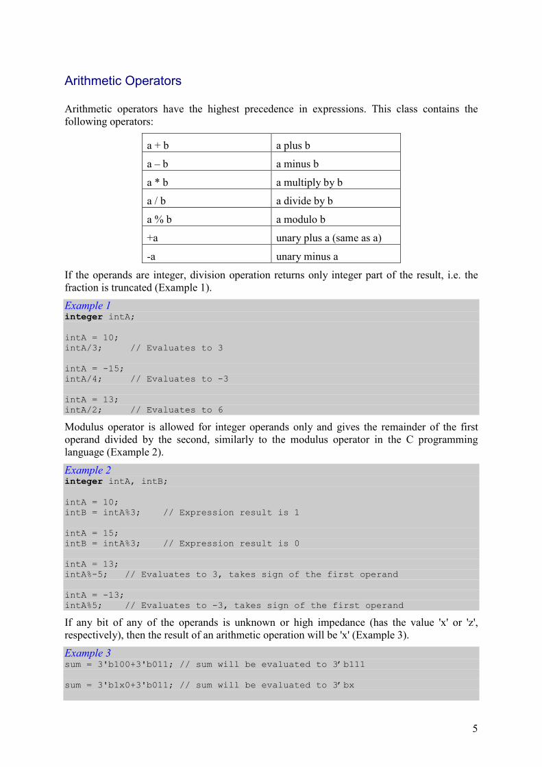
Arithmetic Operators

Arithmetic operators have the highest precedence in expressions. This class contains the following operators:

a + b a plus b

a – b a minus b

a * b a multiply by b

a / b a divide by b

a % b a modulo b

+a unary plus a (same as a)

-a unary minus a

If the operands are integer, division operation returns only integer part of the result, i.e. the fraction is truncated (Example 1).

Example 1 integer intA; intA = 10; intA/3; // Evaluates to 3 intA = -15; intA/4; // Evaluates to -3 intA = 13; intA/2; // Evaluates to 6

Modulus operator is allowed for integer operands only and gives the remainder of the first operand divided by the second, similarly to the modulus operator in the C programming language (Example 2).

Example 2 integer intA, intB; intA = 10; intB = intA%3; // Expression result is 1 intA = 15; intB = intA%3; // Expression result is 0 intA = 13; intA%-5; // Evaluates to 3, takes sign of the first operand intA = -13; intA%5; // Evaluates to -3, takes sign of the first operand

If any bit of any of the operands is unknown or high impedance (has the value 'x' or 'z', respectively), then the result of an arithmetic operation will be 'x' (Example 3).

Example 3 sum = 3'b100+3'b011; // sum will be evaluated to 3’b111 sum = 3'b1x0+3'b011; // sum will be evaluated to 3’bx

6

sum = 4'b110z+4'b0101; // sum will be evaluated to 4’bx

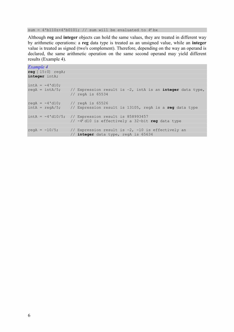
Although reg and integer objects can hold the same values, they are treated in different way by arithmetic operations: a reg data type is treated as an unsigned value, while an integer value is treated as signed (two's complement). Therefore, depending on the way an operand is declared, the same arithmetic operation on the same second operand may yield different results (Example 4).

Example 4 reg [15:0] regA; integer intA; intA = -4'd10; regA = intA/5; // Expression result is –2, intA is an integer data type, // regA is 65534 regA = -4'd10; // regA is 65526 intA = regA/5; // Expression result is 13105, regA is a reg data type intA = -4'd10/5; // Expression result is 858993457 // -4’d10 is effectively a 32-bit reg data type regA = -10/5; // Expression result is –2, -10 is effectively an // integer data type, regA is 65634

7

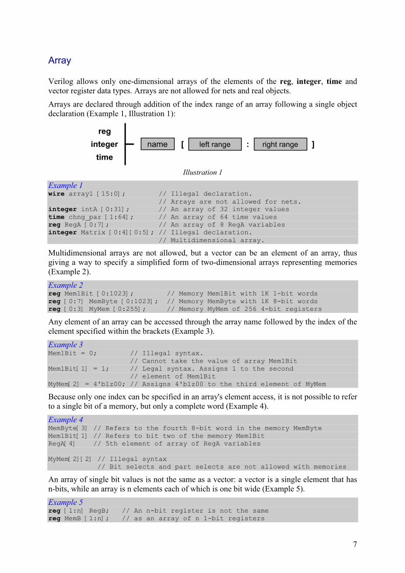
Array

Verilog allows only one-dimensional arrays of the elements of the reg, integer, time and vector register data types. Arrays are not allowed for nets and real objects.

Arrays are declared through addition of the index range of an array following a single object declaration (Example 1, Illustration 1):

reg

integer

time

][ left range :name right range

Illustration 1

Example 1 wire array1 [15:0]; // Illegal declaration. // Arrays are not allowed for nets. integer intA [0:31]; // An array of 32 integer values time chng_par [1:64]; // An array of 64 time values reg RegA [0:7]; // An array of 8 RegA variables integer Matrix [0:4][0:5]; // Illegal declaration. // Multidimensional array.

Multidimensional arrays are not allowed, but a vector can be an element of an array, thus giving a way to specify a simplified form of two-dimensional arrays representing memories (Example 2).

Example 2 reg Mem1Bit [0:1023]; // Memory Mem1Bit with 1K 1-bit words reg [0:7] MemByte [0:1023]; // Memory MemByte with 1K 8-bit words reg [0:3] MyMem [0:255]; // Memory MyMem of 256 4-bit registers

Any element of an array can be accessed through the array name followed by the index of the element specified within the brackets (Example 3).

Example 3 Mem1Bit = 0; // Illegal syntax. // Cannot take the value of array Mem1Bit Mem1Bit[1] = 1; // Legal syntax. Assigns 1 to the second // element of Mem1Bit MyMem[2] = 4'b1z00; // Assigns 4'b1z00 to the third element of MyMem

Because only one index can be specified in an array's element access, it is not possible to refer to a single bit of a memory, but only a complete word (Example 4).

Example 4 MemByte[3] // Refers to the fourth 8-bit word in the memory MemByte Mem1Bit[1] // Refers to bit two of the memory Mem1Bit RegA[4] // 5th element of array of RegA variables MyMem[2][2] // Illegal syntax // Bit selects and part selects are not allowed with memories

An array of single bit values is not the same as a vector: a vector is a single element that has n-bits, while an array is n elements each of which is one bit wide (Example 5).

Example 5 reg [1:n] RegB; // An n-bit register is not the same reg MemB [1:n]; // as an array of n 1-bit registers

8

RegB = 0; // Legal syntax MemB = 0; // Illegal syntax

9

Bit-Select

Bit-select is a form of an expression operand allowing extracting a single bit out of a vector (net or register). The bit is selected by an index, which can be either a static value or an expression (Illustration 1, Example 1). If the index value is unknown or high impedance, then the returned value will also be unknown.

][ indexvector name

Illustration 1

Example 1 reg [7:0] vect1; reg [3:0] vect2; vect1 = 8'b01z0110x; vect2 = 4'b1010; vect1[2]; // Returns 1 vect1[8]; // If the value of index is out of // bounds, then vect1[index]returns x. vect1[4*vect1[6] + vect2[1]]; // In this case index=4*1+1=5, // then vect1[index] returns z. vect1[vect1[0] & vect2[1]]; // If the value of index evaluates to x, // then vect1[index] returns x. vect2[0]; // Returns 0

It is not allowed to specify bit-select of a register declared as a real or realtime.

10

Bit-wise Operators

Bit-wise operations perform bit-wise manipulations on operands, i.e. the value of each bit of the result is determined by applying a logical operator to corresponding bits of both operands.

There are five bit-wise operators and the table below presents the results of applying them to all possible combinations of bit values:

and

& 0 1 x z

or

| 0 1 x z

xor

^ 0 1 x z

0 0 0 0 0 0 0 1 x x 0 0 1 x x

1 0 1 x x 1 1 1 1 1 1 1 0 x x

x 0 x x x x x 1 x x x x x x x

z 0 x x x z x 1 x x z x x x x

xnor

^~ ~^ 0 1 x z

not

~

0 1 0 x x 0 1

1 0 1 x x 1 0

x x x x x x x

z x x x x z x

Examples:

Example 1 wire A, B, C, D; reg [3:0] Vect1, Vect2; wire [3:0] Vect3, Vect4; // C = 1'b0 D = 1'b1 assign A = D&C; // A = 0 assign B = C^D; // B = 1 // Vect3 = 4'b0z1x Vect4 = 4'b0011 initial begin Vect1 = Vect3|Vect4; // Vect1 = 0x11 Vect2 = Vect3~^Vect4; // Vect2 = 1x1x end

If one of the operands is shorter than the other, it is filled with zeros in the most significant positions to match the sizes (Example 2).

Example 2 reg [3:0] Vect1, Vect2; wire [3:0] Vect3; wire [1:0] Vect4; // Vect3 = 4'b1010 Vect4 = 2'b11 initial

11

begin Vect1 = Vect3|Vect4; // Vect1 = 1011 Vect2 = Vect3~^Vect4; // Vect2 = 0110 end

The main difference between bit-wise and logical operators in Verilog HDL is the size of the result: in bit-wise expressions the result has the same size as the bigger operand, while in logical expressions the result is always a single bit.

12

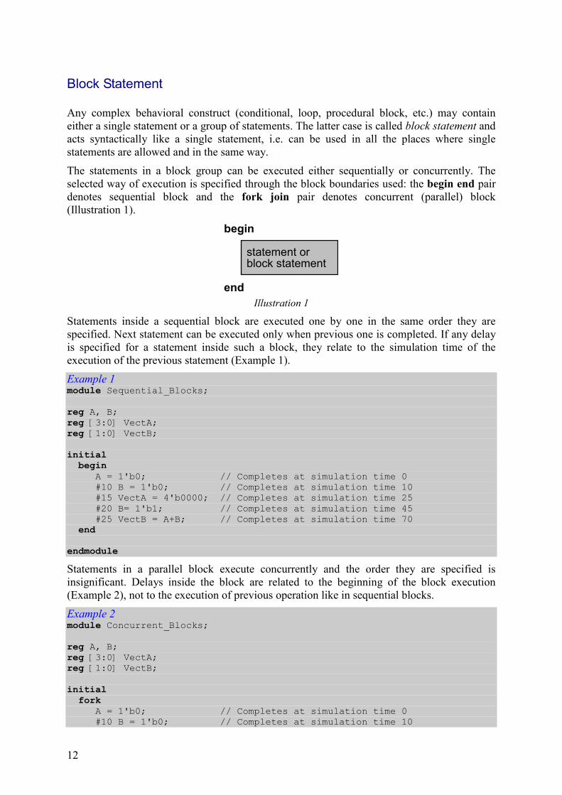
Block Statement

Any complex behavioral construct (conditional, loop, procedural block, etc.) may contain either a single statement or a group of statements. The latter case is called block statement and acts syntactically like a single statement, i.e. can be used in all the places where single statements are allowed and in the same way.

The statements in a block group can be executed either sequentially or concurrently. The selected way of execution is specified through the block boundaries used: the begin end pair denotes sequential block and the fork join pair denotes concurrent (parallel) block (Illustration 1).

begin

end

statement orblock statement

Illustration 1

Statements inside a sequential block are executed one by one in the same order they are specified. Next statement can be executed only when previous one is completed. If any delay is specified for a statement inside such a block, they relate to the simulation time of the execution of the previous statement (Example 1).

Example 1 module Sequential_Blocks; reg A, B; reg [3:0] VectA; reg [1:0] VectB; initial begin A = 1'b0; // Completes at simulation time 0 #10 B = 1'b0; // Completes at simulation time 10 #15 VectA = 4'b0000; // Completes at simulation time 25 #20 B= 1'b1; // Completes at simulation time 45 #25 VectB = A+B; // Completes at simulation time 70 end endmodule

Statements in a parallel block execute concurrently and the order they are specified is insignificant. Delays inside the block are related to the beginning of the block execution (Example 2), not to the execution of previous operation like in sequential blocks.

Example 2 module Concurrent_Blocks; reg A, B; reg [3:0] VectA; reg [1:0] VectB; initial fork A = 1'b0; // Completes at simulation time 0 #10 B = 1'b0; // Completes at simulation time 10

13

#15 VectA = 4'b0000; // Completes at simulation time 15 #20 B= 1'b1; // Completes at simulation time 20 #25 VectB = A+B; // Completes at simulation time 25 join endmodule

Block statements can be assigned individual names. The name is specified after a semicolon following the begin or fork keyword (Illustration 2).

block namebegin

fork

end

join

:

statement orblock statement

Illustration 2

Apart from enhancing readability of the code, naming blocks allows declaring local registers (Example 3) and disabling the block (Example 4)

Example 3 initial begin : Init_Vect // An integer K and MSB are static // and local to Init_Vect integer K, MSB; MSB = 8; K = 0; repeat (MSB) begin // Initialize vector elements Vector[K] = 1'b0; K = K + 1; end end

Example 4 initial begin : Clock_Generator parameter Half_Cycle = 10, Start_Value = 1'b0; Clk = Start_Value; begin : Generating forever begin #Half_Cycle Clk = ~Clk; // Named block can be disabled, // i.e., its execution can be stopped. if ($time == 200) disable Generating; end end end

14

Blocking Assignment

See procedural assignment.

15

Case Statement

The case statement is a multiple branch conditional statement. An expression, which is often a single signal or variable, is evaluated and compared to the expressions (usually values) assigned to branches (Illustration 1). The branch expressions are compared with the main in the order in which they are given. If one of the expressions matches the main expression, then the respective branch is executed. An optional default branch, representing the values that are not listed, can be used. It is denoted by the keyword default instead of a branch expression (Example 1). If there is no match of expressions and there is no default branch, no statements inside the case is executed.

casex

case item

expressionz

endcase

( )

Illustration 1

Example 1 module Mux4to1 (D0, D1, D2, D3, Sel, Result); input [1:0] D0, D1, D2, D3, Sel; output [1:0] Result; reg [1:0] Result;

always @(D0 or D1 or D2 or D3 or Sel) begin

case (Sel) 0 : Result = D0; 1 : Result = D1; 2 : Result = D2; 3 : Result = D3; default : Result = 2'bx; endcase end

endmodule

In the case statement the match must be an exact one, i.e. all the values in all the bits of both expressions must be the same with respect to all possible four logical values, including unknown and high impedance. In practical terms it means that in a case statement an insignificant bits may not be represented by ‘x’, but it should contain all four alternatives for a particular branch (Example 2).

Example 2 //improper reference to insignificant bit case (OpCode) 3'b11x : AX = BX + CX; . . .; endcase

//this branch will be executed only when the LSB is ‘x’, //even though the designer meant ‘insignificant’ //corrected version: case (OpCode) 3’b110, 3’b111, 3'b11x, 3’b11z : AX = BX + CX;

16

. . .; endcase

Listing all possible alternatives may not be viable, therefore Verilog offers two extensions to the case statement, allowing handling of don’t care conditions more naturally. The syntax of such modified case statement is the same as of the original one, except that the casez or casex keywords are used instead of case.

The casez statement (Example 3) treats high-impedance values as don’t cares, while casex (Example 4) treats this way both high-impedance and unknown value. All don’t care bits are simply not considered in the comparisons of expressions. Additionally, the high impedance value can be specified with the '?' character (Example 3).

Example 3 module Counter (Din, Clk, Clr, Load, UpDn, Dout); input [3:0] Din; input Clk, Clr, Load, UpDn; output [3:0] Dout; reg [3:0] Dout; always @ (posedge Clk) begin

casez ({Clr, Load, UpDn}) 3'b0zz : Dout = 4'b0; 3'b11? : Dout = Din; 3'b101 : Dout = Dout + 1; 3'b100 : Dout = Dout - 1; default : Dout = 4'bx; endcase end

endmodule

Example 4 module ShiftReg (Outs, Ins, Clk, Clr, Set, Shl, Shr); input [7:0] Ins; input Clk, Clr, Set, Shl, Shr; output [7:0] Outs; reg [7:0] Outs; initial

Outs = 0; always @(posedge Clk) casex ({Clr, Set, Shl, Shr}) 4'b1xxx : Outs = 0; 4'bx1xx : Outs = {Size{1'b1}}; 4'bxx1x : Outs = Outs << 1; 4'bxxx1 : Outs = Outs >> 1; default : Outs = Ins; endcase endmodule

17

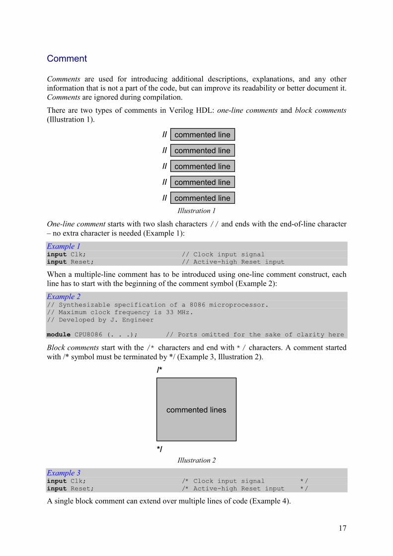
Comment

Comments are used for introducing additional descriptions, explanations, and any other information that is not a part of the code, but can improve its readability or better document it. Comments are ignored during compilation.

There are two types of comments in Verilog HDL: one-line comments and block comments (Illustration 1).

commented line//

commented line//

commented line//

commented line//

commented line//

Illustration 1

One-line comment starts with two slash characters // and ends with the end-of-line character – no extra character is needed (Example 1):

Example 1 input Clk; // Clock input signal input Reset; // Active-high Reset input

When a multiple-line comment has to be introduced using one-line comment construct, each line has to start with the beginning of the comment symbol (Example 2):

Example 2 // Synthesizable specification of a 8086 microprocessor. // Maximum clock frequency is 33 MHz. // Developed by J. Engineer module CPU8086 (. . .); // Ports omitted for the sake of clarity here

Block comments start with the /* characters and end with */ characters. A comment started

with /* symbol must be terminated by */ (Example 3, Illustration 2).

commented lines

/*

*/

Illustration 2

Example 3 input Clk; /* Clock input signal */ input Reset; /* Active-high Reset input */

A single block comment can extend over multiple lines of code (Example 4).

18

Example 4 /* Synthesizable specification of a 8086 microprocessor. Maximum clock frequency is 33 MHz. Developed by J. Engineer */ module CPU8086 (. . .); // Ports omitted for the sake of clarity here

A block comment cannot be nested in another block comment, but you can nest one-line comments in block comments.

19

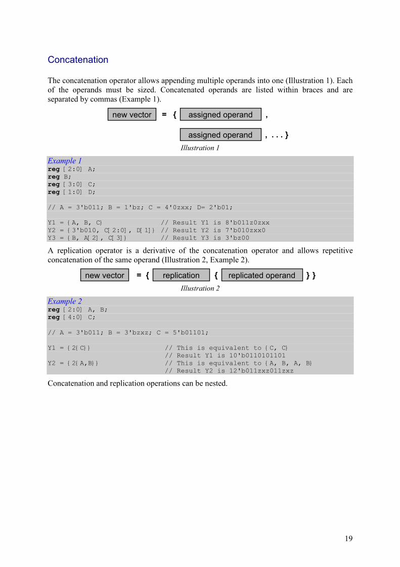
Concatenation

The concatenation operator allows appending multiple operands into one (Illustration 1). Each of the operands must be sized. Concatenated operands are listed within braces and are separated by commas (Example 1).

new vector

}

{

,

= assigned operand ,

assigned operand . . .

Illustration 1

Example 1 reg [2:0] A; reg B; reg [3:0] C; reg [1:0] D; // A = 3'b011; B = 1'bz; C = 4'0zxx; D= 2'b01; Y1 = {A, B, C} // Result Y1 is 8'b011z0zxx Y2 = {3'b010, C[2:0], D[1]} // Result Y2 is 7'b010zxx0 Y3 = {B, A[2], C[3]} // Result Y3 is 3'bz00

A replication operator is a derivative of the concatenation operator and allows repetitive concatenation of the same operand (Illustration 2, Example 2).

new vector }{= replication ,replicated operand{ }

Illustration 2

Example 2 reg [2:0] A, B; reg [4:0] C; // A = 3'b011; B = 3'bzxz; C = 5'b01101; Y1 = {2{C}} // This is equivalent to {C, C} // Result Y1 is 10'b0110101101 Y2 = {2{A,B}} // This is equivalent to {A, B, A, B} // Result Y2 is 12'b011zxz011zxz

Concatenation and replication operations can be nested.

20

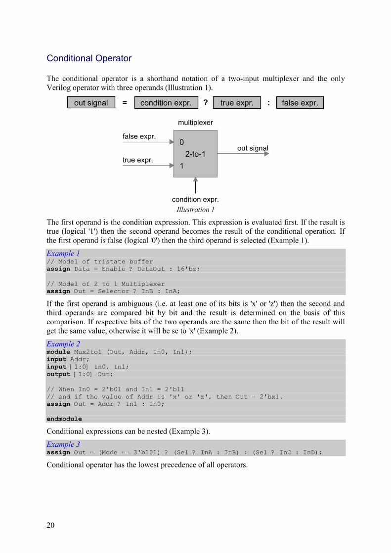
Conditional Operator

The conditional operator is a shorthand notation of a two-input multiplexer and the only Verilog operator with three operands (Illustration 1).

out signal := condition expr. true expr.? false expr.

false expr.

true expr.

condition expr.

out signal

multiplexer

0

1

2-to-1

Illustration 1

The first operand is the condition expression. This expression is evaluated first. If the result is true (logical '1') then the second operand becomes the result of the conditional operation. If the first operand is false (logical '0') then the third operand is selected (Example 1).

Example 1 // Model of tristate buffer assign Data = Enable ? DataOut : 16'bz; // Model of 2 to 1 Multiplexer assign Out = Selector ? InB : InA;

If the first operand is ambiguous (i.e. at least one of its bits is 'x' or 'z') then the second and third operands are compared bit by bit and the result is determined on the basis of this comparison. If respective bits of the two operands are the same then the bit of the result will get the same value, otherwise it will be se to 'x' (Example 2).

Example 2 module Mux2to1 (Out, Addr, In0, In1); input Addr; input [1:0] In0, In1; output [1:0] Out; // When In0 = 2'b01 and In1 = 2'b11 // and if the value of Addr is 'x' or 'z', then Out = 2'bx1. assign Out = Addr ? In1 : In0; endmodule

Conditional expressions can be nested (Example 3).

Example 3 assign Out = (Mode == 3'b101) ? (Sel ? InA : InB) : (Sel ? InC : InD);

Conditional operator has the lowest precedence of all operators.

21

Continuous Assignment

Continuous assignment is the basic statement in dataflow modeling. It defines a driver for a net and is executed whenever any of the operands in the right-hand side expression changes its value (hence the 'continuous' in its name). The new value of the expression is calculated and assigned to the net specified on the left-hand side.

Each continuous assignment statement begins with the assign keyword, followed by optional strength and delay specifications and the assignment itself (Illustration 1).

name ;= strength delay assignmentassign

# delay time specification

( )strength0,strength1

Illustration 1

As a dataflow-type statement, continuous assignment is specified outside procedural blocks, i.e. at the topmost level of a module. Inside a procedural block, only procedural assignments can be used.

The left-hand side of a continuous assignment must be a net (scalar or vector) or a concatenation of nets (Example 1). It is not allowed to use registers as targets of continuous assignments.

Example 1 module Comparator (AequalB, AlessB, AgreaterB, A, B); input A, B; output AequalB, AlessB, AgreaterB; assign AequalB = A~^B; assign AlessB = ~A&B; assign AgreaterB = A&~B; endmodule module FullAdderVer1 (Cout, Sum, A, B, Cin); input [1:0] A, B; input Cin; output [1:0] Sum; output Cout; assign {Cout,Sum} = A + B + Cin; endmodule

The expression on the right-hand side of a continuous assignment may contain operands that are nets, registers or function calls (Example 2).

Example 2 module SimpleCPU (A, B, C, Result);

22

input [3:0] A, B; input [2:0] C; output [4:0] Result; function [4:0] ALU; input [3:0] InA, InB; input [2:0] Mode; reg [4:0] Temp; begin case (Mode) 3'b000 : Temp = InA; 3'b001 : Temp = InA + InB; 3'b010 : Temp = InA - InB; 3'b011 : Temp = ~InA + 1; 3'b100 : Temp = ~InB + 1; 3'b101 : Temp = InB; 3'b110 : Temp = InA << 1; 3'b111 : Temp = InB >> 1; default : Temp = 4'bz; endcase ALU = Temp; end endfunction assign Result = ALU (A, B, C); endmodule

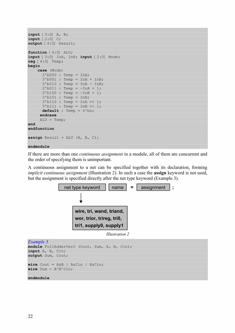
If there are more than one continuous assignment in a module, all of them are concurrent and the order of specifying them is unimportant.

A continuous assignment to a net can be specified together with its declaration, forming implicit continuous assignment (Illustration 2). In such a case the assign keyword is not used, but the assignment is specified directly after the net type keyword (Example 3).

name ;= assignmentnet type keyword

wire, tri, wand, triand,

wor, trior, trireg, tri0,

tri1, supply0, supply1

Illustration 2

Example 3 module FullAdderVer2 (Cout, Sum, A, B, Cin); input A, B, Cin; output Sum, Cout; wire Cout = A&B | A&Cin | B&Cin; wire Sum = A^B^Cin; endmodule

23

Data Types

There are three main classes of data types in Verilog HDL: nets (Example 1), registers (Example 2) and events (Example 3). Detailed information on the three classes and all types covered by them can be found in respective topics: Net Data Types, Register Data Types and Events.

Example 1 // The net data types: wire A, B, C; // Default net data type wand A_WiredAnd; wor B_WiredOr; supply0 Ground; supply1 Power; wire [31:0] Vector1; assign A = 1'bz; assign Vector1 = 32'haf101;

Example 2 // The register data types: reg RegA, RegB; reg [7:0] Vector2; reg [15:0] Memory [31:0]; integer Iteration, Value; time T_Hold; realtime T_Setup; real Value1, Value2 initial begin RegA = 'bz; Vector2 = 8'b111z010x; Iteration = 32; T_Hold = 10; T_Setup = 12.25; Value1 = 1.5; Value2 = 2.75e-2; end

Example 3 // The event data type: event Unknown_Value, OK_Value; always @ (Data) begin if (^Data === 1'bx) -> Unknown_Value; else -> OK_Value; end

24

Delays

A delay is specified as one or more values preceded by a hash ('#') symbol (Illustration 1). In primitive and module instantiations delay is specified between the primitive (or module) name and the instance name (Illustration 2). Delays of the assignments can be specified either preceding the left or right hand side of the assignment (Illustration 3).

# delay value

Illustration 1

delayprimitive or module name # instance name

Illustration 2

delay =

delay

expression# left side of assignment

left side of assignment = # expression

Illustration 3

If no delay is specified for a particular instance or assignment it is implicitly assumed that the delay is zero.

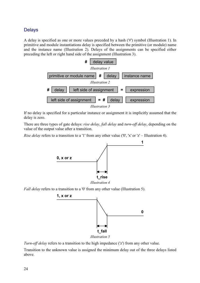
There are three types of gate delays: rise delay, fall delay and turn-off delay, depending on the value of the output value after a transition.

Rise delay refers to a transition to a '1' from any other value ('0', 'x' or 'z' – Illustration 4).

0, x or z

1

t_rise

Illustration 4

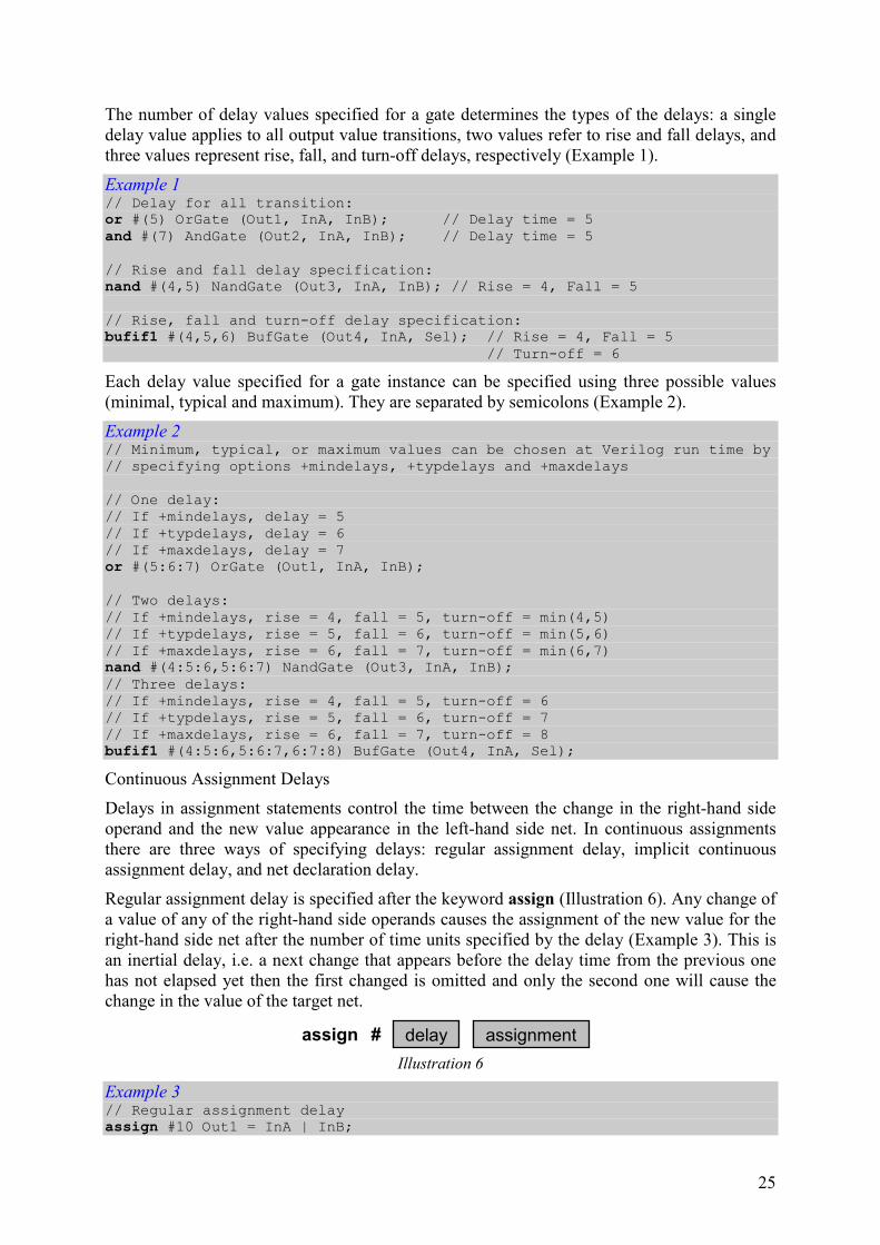
Fall delay refers to a transition to a '0' from any other value (Illustration 5).

1, x or z

0

t_fall

Illustration 5

Turn-off delay refers to a transition to the high impedance ('z') from any other value.

Transition to the unknown value is assigned the minimum delay out of the three delays listed above.

25

The number of delay values specified for a gate determines the types of the delays: a single delay value applies to all output value transitions, two values refer to rise and fall delays, and three values represent rise, fall, and turn-off delays, respectively (Example 1).

Example 1 // Delay for all transition: or #(5) OrGate (Out1, InA, InB); // Delay time = 5 and #(7) AndGate (Out2, InA, InB); // Delay time = 5 // Rise and fall delay specification: nand #(4,5) NandGate (Out3, InA, InB); // Rise = 4, Fall = 5 // Rise, fall and turn-off delay specification: bufif1 #(4,5,6) BufGate (Out4, InA, Sel); // Rise = 4, Fall = 5 // Turn-off = 6

Each delay value specified for a gate instance can be specified using three possible values (minimal, typical and maximum). They are separated by semicolons (Example 2).

Example 2 // Minimum, typical, or maximum values can be chosen at Verilog run time by // specifying options +mindelays, +typdelays and +maxdelays // One delay: // If +mindelays, delay = 5 // If +typdelays, delay = 6 // If +maxdelays, delay = 7 or #(5:6:7) OrGate (Out1, InA, InB); // Two delays: // If +mindelays, rise = 4, fall = 5, turn-off = min(4,5) // If +typdelays, rise = 5, fall = 6, turn-off = min(5,6) // If +maxdelays, rise = 6, fall = 7, turn-off = min(6,7) nand #(4:5:6,5:6:7) NandGate (Out3, InA, InB); // Three delays: // If +mindelays, rise = 4, fall = 5, turn-off = 6 // If +typdelays, rise = 5, fall = 6, turn-off = 7 // If +maxdelays, rise = 6, fall = 7, turn-off = 8 bufif1 #(4:5:6,5:6:7,6:7:8) BufGate (Out4, InA, Sel);

Continuous Assignment Delays

Delays in assignment statements control the time between the change in the right-hand side operand and the new value appearance in the left-hand side net. In continuous assignments there are three ways of specifying delays: regular assignment delay, implicit continuous assignment delay, and net declaration delay.

Regular assignment delay is specified after the keyword assign (Illustration 6). Any change of a value of any of the right-hand side operands causes the assignment of the new value for the right-hand side net after the number of time units specified by the delay (Example 3). This is an inertial delay, i.e. a next change that appears before the delay time from the previous one has not elapsed yet then the first changed is omitted and only the second one will cause the change in the value of the target net.

delay# assignmentassign

Illustration 6

Example 3 // Regular assignment delay assign #10 Out1 = InA | InB;

26

assign #15 Out2 = (InA | InB) & InC;

A delay can also be specified also for an implicit continuous assignment (Illustration 7). It has the same effect as a regular assignment delay, but is more compact (Example 4).

delay implicit continuous assignment#net type

Illustration7

Example 4 // Implicit continuous assignment delay wire #10 Out1 = InA | InB; // same as wire Out1; assign #10 Out1 = InA | InB;

A delay can be specified for a net itself, directly in its declaration. In such a case the delay is specified between the net type and name (Illustration 8) and will apply to all assignments and instantiations with this net (Example 5).

delaynet type # net name

Illustration 8

Example 5 // Net delay wire #10 Out1; assign Out1 = InA | InB; // same effect as wire Out1; assign #10 Out1 = InA | InB;

27

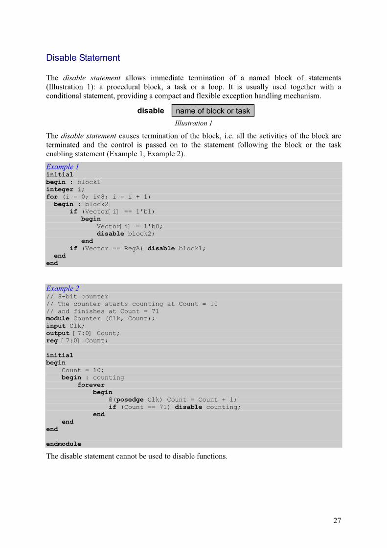
Disable Statement

The disable statement allows immediate termination of a named block of statements (Illustration 1): a procedural block, a task or a loop. It is usually used together with a conditional statement, providing a compact and flexible exception handling mechanism.

name of block or taskdisable

Illustration 1

The disable statement causes termination of the block, i.e. all the activities of the block are terminated and the control is passed on to the statement following the block or the task enabling statement (Example 1, Example 2).

Example 1 initial begin : block1 integer i; for (i = 0; i<8; i = i + 1) begin : block2 if (Vector[i] == 1'b1) begin Vector[i] = 1'b0; disable block2; end if (Vector == RegA) disable block1; end end

Example 2 // 8-bit counter // The counter starts counting at Count = 10 // and finishes at Count = 71 module Counter (Clk, Count); input Clk; output [7:0] Count; reg [7:0] Count; initial begin Count = 10; begin : counting forever begin @(posedge Clk) Count = Count + 1; if (Count == 71) disable counting; end end end

endmodule

The disable statement cannot be used to disable functions.

28

Equality Operators

Equality operators are separated from relational operators for two reasons: they have lower precedence and may cope with ambiguous values in a different way.

There are four equality operators:

a === b a equal to b, including x and z

a !== b a not equal to b, including x and z

a == b a equal to b, result may be unknown

a != b a not equal to b, result may be unknown

Similarly to relational operators, equality operator yields a single-bit result: '0' if the specified relation is false or '1' if the relation holds true. There are, however, differences in coping with unknown and high impedance values in operands.

The first two operators (=== and !==) are called case equality operators and compare two operands bit by bit considering all four possible values ('0', '1', 'x', and 'z') as valid, i.e. two operands will be considered equal if all their bits have the same values (Example 1).

Example 1 reg [3:0] regA, regB; // regA = 4'b1100 regB = 4'b0011 regA===regB // Evaluates to 0 regA!==regB // Evaluates to 1 // regA = 4'b1xz0; regB = 4'b1100; regA===regB // Evaluates to 0 regA!==regB // Evaluates to 1 // regA = 4'b1xz0; regB = 4'b1xz0; regA===regB // Evaluates to 1 regA!==regB // Evaluates to 0 // regA = 4'b1100; regB = 4'b1100; regA===regB // Evaluates to 1 regA!==regB // Evaluates to 0

The other two operators (== and !=) are called logical equality and comparison verifies equality of the values '0' and '1' only. Whenever any bit is 'x' or 'z', the result will be 'x', even if the ambiguous bit is the same in both operands (Example 2)

This example has the same input values but produces different results.

Example 2 reg [3:0] regA, regB; // regA = 4'b1100 regB = 4'b0011 regA==regB // Evaluates to 0 regA!=regB // Evaluates to 1 // regA = 4'b1xz0; regB = 4'b1100; regA==regB // Evaluates to x regA!=regB // Evaluates to x // regA = 4'b1xz0; regB = 4'b1xz0;

29

regA==regB // Evaluates to x regA!=regB // Evaluates to x // regA = 4'b1100; regB = 4'b1100; regA==regB // Evaluates to 1 regA!=regB // Evaluates to 0

30

Events

Events provide an alternative (to delays) timing control over the execution of statements. In its simplest form an event is a change of value on a net or register and is referred to through the symbol @ followed by the net or register name (Illustration 1). The statement that follows an event control is executed only when an event on the specified object is detected (Example 1).

net or register name@

Illustration 1

Two types of events are distinguished and can be specified in event control: rising edge and falling edge. The former one is specified by the posedge keyword, while the latter by the negedge keyword. The interpretation of edges is presented at Illustration 2.

To

From 0 1 x z

0 No edge posedge posedge posedge

1 negedge No edge negedge negedge

x negedge posedge No edge No edge

z negedge posedge No edge No edge

Illustration 2

Example 1 // Regular event control // Positive edge-triggered D flip-flop // with asynchronous preset module D_FlipFlop (D, Clk, Preset, Q, Qbar); input D, Clk, Preset; output Q, Qbar; reg Q, Qbar; always @ (posedge Clk) begin Q = D; Qbar = ~D; end always @ (Preset) begin if (Preset) begin assign Q = 1'b1; assign Qbar = 1'b0; end else begin deassign Q; deassign Qbar; end end endmodule

31

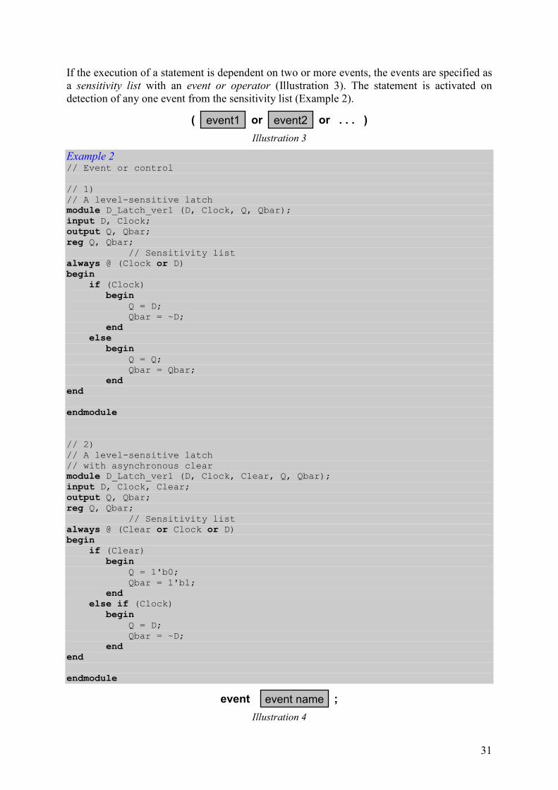
If the execution of a statement is dependent on two or more events, the events are specified as a sensitivity list with an event or operator (Illustration 3). The statement is activated on detection of any one event from the sensitivity list (Example 2).

event1 oror( )event2 . . .

Illustration 3

Example 2 // Event or control // 1) // A level-sensitive latch module D_Latch_ver1 (D, Clock, Q, Qbar); input D, Clock; output Q, Qbar; reg Q, Qbar; // Sensitivity list always @ (Clock or D) begin if (Clock) begin Q = D; Qbar = ~D; end else begin Q = Q; Qbar = Qbar; end end endmodule

// 2) // A level-sensitive latch // with asynchronous clear module D_Latch_ver1 (D, Clock, Clear, Q, Qbar); input D, Clock, Clear; output Q, Qbar; reg Q, Qbar; // Sensitivity list always @ (Clear or Clock or D) begin if (Clear) begin Q = 1'b0; Qbar = 1'b1; end else if (Clock) begin Q = D; Qbar = ~D; end end endmodule

event nameevent ;

Illustration 4

32

The events presented earlier are implicit events. Verilog HDL offers another form of events, available through separate objects of the type event (Illustration 4). Such events are called named events and do not hold any data. They can, however, be triggered explicitly (Illustration 5) and used for the control of behavioral statements in the same way as implicit events (Example 3).

event name->

Illustration 5

Example 3 // Named event control module DetectUnknown (Data, Control); input [3:0] Data; output Control; reg Control; event Unknown_Value, OK_Value; always @ (Data) begin if (^Data === 1'bx) -> Unknown_Value; else -> OK_Value; end always @ (Unknown_Value) begin $display ("Unknown value on the data bus!"); Control = 1'b0; end always @ (OK_Value) begin $display ("OK value on the data bus!"); Control = 1'b1; end endmodule

33

Expressions

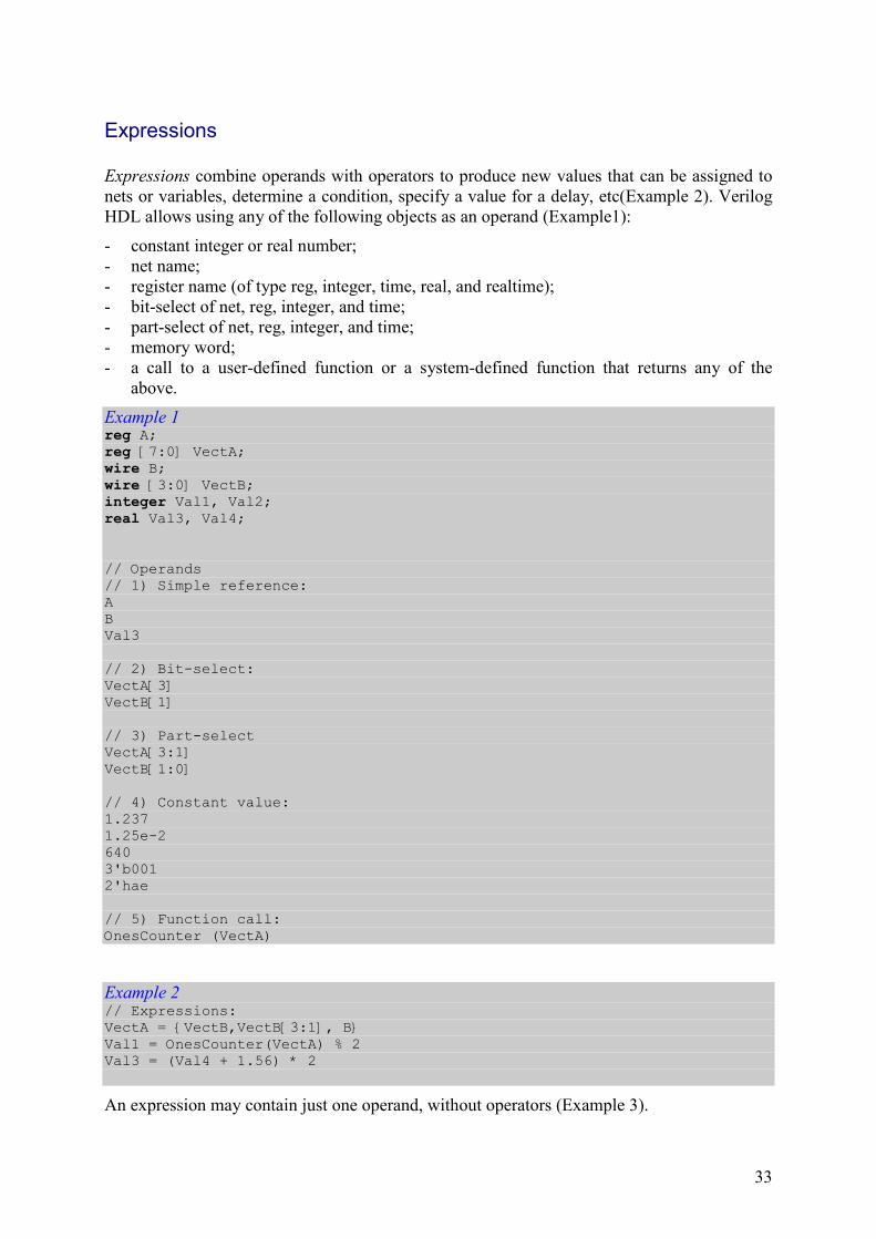
Expressions combine operands with operators to produce new values that can be assigned to nets or variables, determine a condition, specify a value for a delay, etc(Example 2). Verilog HDL allows using any of the following objects as an operand (Example1):

- constant integer or real number; - net name; - register name (of type reg, integer, time, real, and realtime); - bit-select of net, reg, integer, and time; - part-select of net, reg, integer, and time; - memory word; - a call to a user-defined function or a system-defined function that returns any of the

above.

Example 1 reg A; reg [7:0] VectA; wire B; wire [3:0] VectB; integer Val1, Val2; real Val3, Val4; // Operands // 1) Simple reference: A B Val3 // 2) Bit-select: VectA[3] VectB[1] // 3) Part-select VectA[3:1] VectB[1:0] // 4) Constant value: 1.237 1.25e-2 640 3'b001 2'hae // 5) Function call: OnesCounter (VectA)

Example 2 // Expressions: VectA = {VectB,VectB[3:1], B} Val1 = OnesCounter(VectA) % 2 Val3 = (Val4 + 1.56) * 2

An expression may contain just one operand, without operators (Example 3).

34

Example 3 VectA = 2'h10 Val3 = 1.33 B = 1'bx

35

For Loop

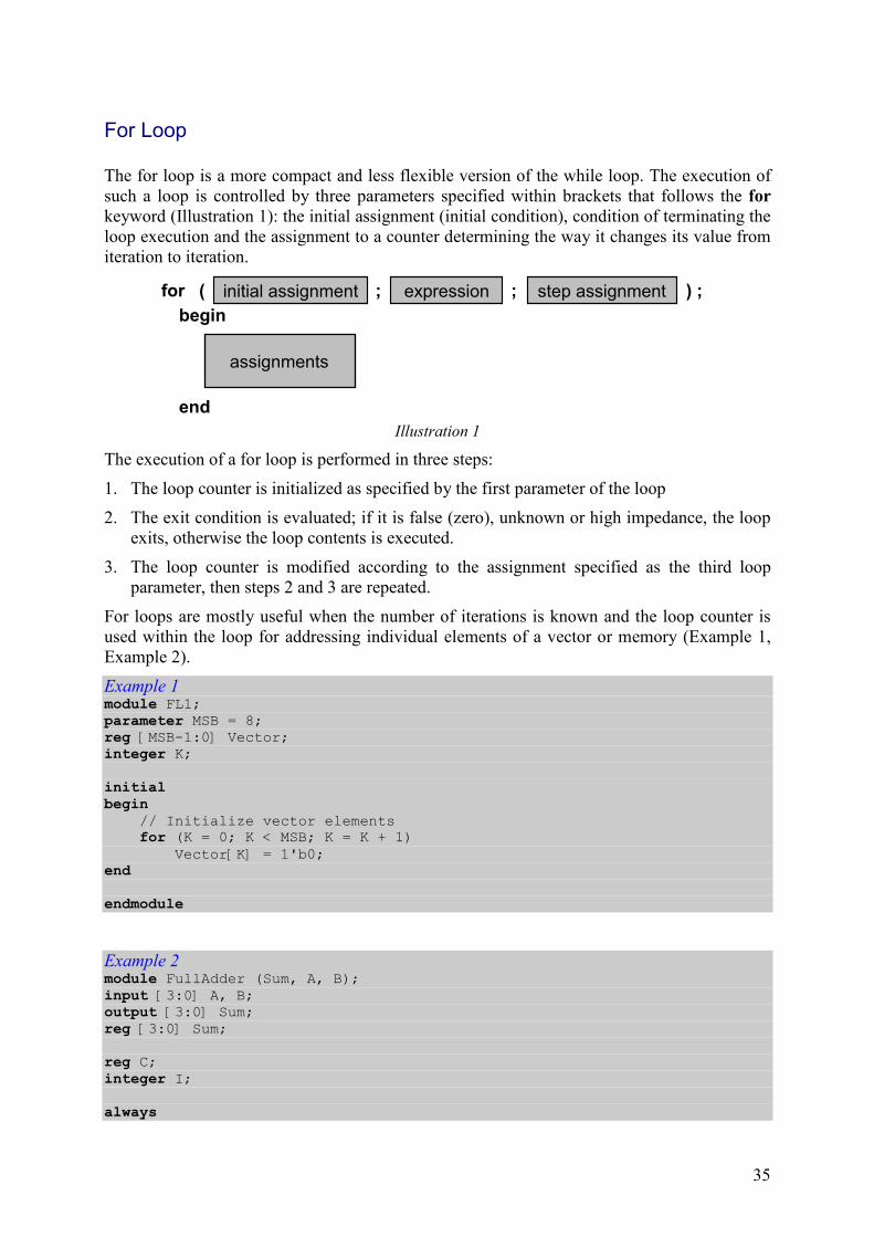
The for loop is a more compact and less flexible version of the while loop. The execution of such a loop is controlled by three parameters specified within brackets that follows the for keyword (Illustration 1): the initial assignment (initial condition), condition of terminating the loop execution and the assignment to a counter determining the way it changes its value from iteration to iteration.

begin

end

assignments

for initial assignment expression step assignment( ) ;; ;

Illustration 1

The execution of a for loop is performed in three steps:

1. The loop counter is initialized as specified by the first parameter of the loop

2. The exit condition is evaluated; if it is false (zero), unknown or high impedance, the loop exits, otherwise the loop contents is executed.

3. The loop counter is modified according to the assignment specified as the third loop parameter, then steps 2 and 3 are repeated.

For loops are mostly useful when the number of iterations is known and the loop counter is used within the loop for addressing individual elements of a vector or memory (Example 1, Example 2).

Example 1 module FL1; parameter MSB = 8; reg [MSB-1:0] Vector; integer K; initial begin // Initialize vector elements for (K = 0; K < MSB; K = K + 1) Vector[K] = 1'b0; end endmodule

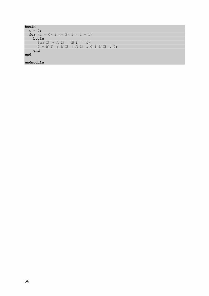
Example 2 module FullAdder (Sum, A, B); input [3:0] A, B; output [3:0] Sum; reg [3:0] Sum; reg C; integer I; always

36

begin

C = 0; for (I = 0; I <= 3; I = I + 1) begin Sum[I] = A[I] ^ B[I] ^ C; C = A[I] & B[I] | A[I] & C | B[I] & C; end end

endmodule

37

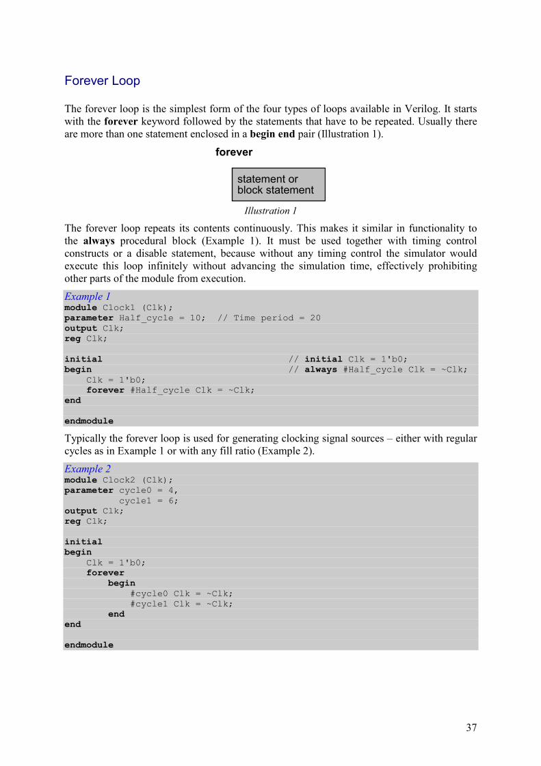
Forever Loop

The forever loop is the simplest form of the four types of loops available in Verilog. It starts with the forever keyword followed by the statements that have to be repeated. Usually there are more than one statement enclosed in a begin end pair (Illustration 1).

statement orblock statement

forever

Illustration 1

The forever loop repeats its contents continuously. This makes it similar in functionality to the always procedural block (Example 1). It must be used together with timing control constructs or a disable statement, because without any timing control the simulator would execute this loop infinitely without advancing the simulation time, effectively prohibiting other parts of the module from execution.

Example 1 module Clock1 (Clk); parameter Half_cycle = 10; // Time period = 20 output Clk; reg Clk; initial // initial Clk = 1'b0; begin // always #Half_cycle Clk = ~Clk; Clk = 1'b0; forever #Half_cycle Clk = ~Clk; end endmodule

Typically the forever loop is used for generating clocking signal sources – either with regular cycles as in Example 1 or with any fill ratio (Example 2).

Example 2 module Clock2 (Clk); parameter cycle0 = 4, cycle1 = 6; output Clk; reg Clk; initial begin Clk = 1'b0; forever begin #cycle0 Clk = ~Clk; #cycle1 Clk = ~Clk; end end endmodule

38

Function

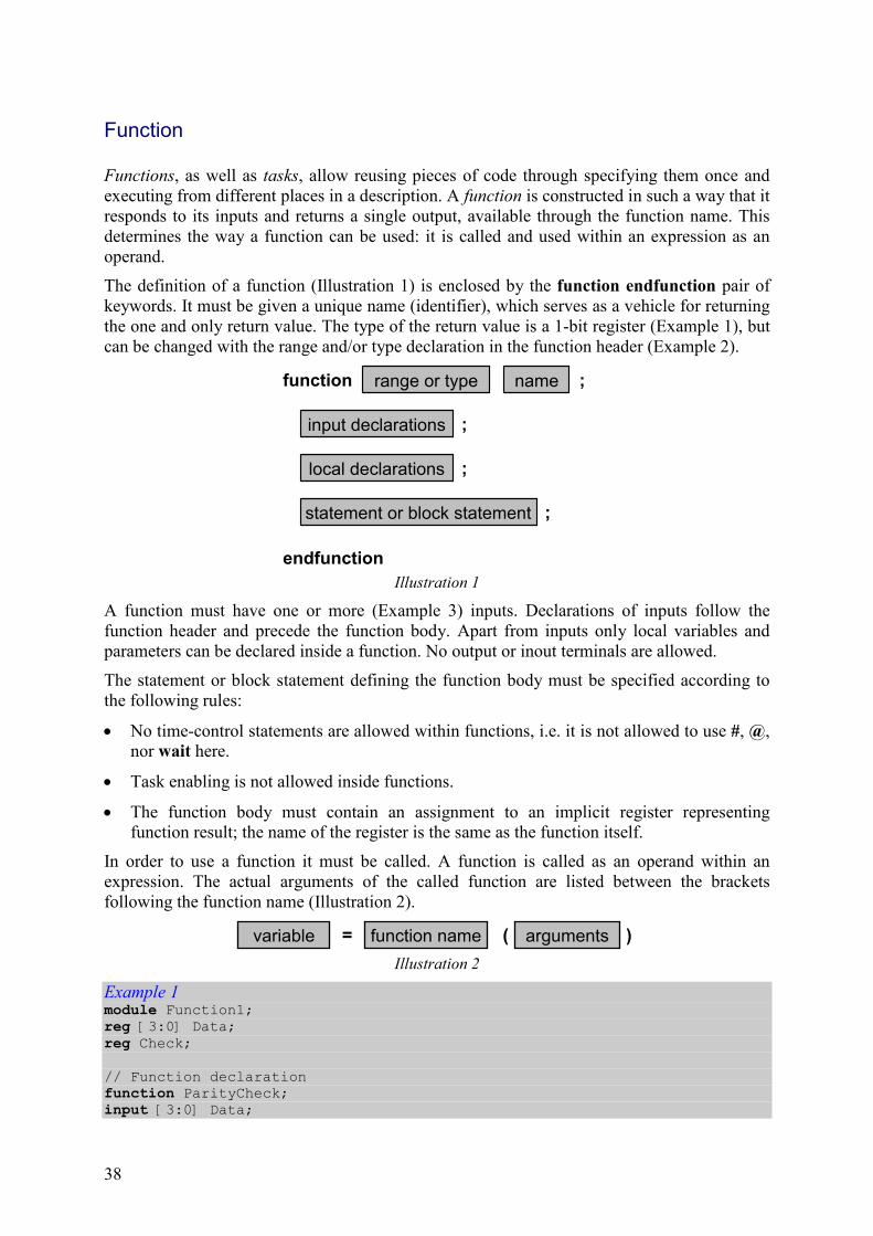
Functions, as well as tasks, allow reusing pieces of code through specifying them once and executing from different places in a description. A function is constructed in such a way that it responds to its inputs and returns a single output, available through the function name. This determines the way a function can be used: it is called and used within an expression as an operand.

The definition of a function (Illustration 1) is enclosed by the function endfunction pair of keywords. It must be given a unique name (identifier), which serves as a vehicle for returning the one and only return value. The type of the return value is a 1-bit register (Example 1), but can be changed with the range and/or type declaration in the function header (Example 2).

endfunction

function range or type

input declarations ;

;name

local declarations ;

statement or block statement ;

Illustration 1

A function must have one or more (Example 3) inputs. Declarations of inputs follow the function header and precede the function body. Apart from inputs only local variables and parameters can be declared inside a function. No output or inout terminals are allowed.

The statement or block statement defining the function body must be specified according to the following rules:

• No time-control statements are allowed within functions, i.e. it is not allowed to use #, @, nor wait here.

• Task enabling is not allowed inside functions.

• The function body must contain an assignment to an implicit register representing function result; the name of the register is the same as the function itself.

In order to use a function it must be called. A function is called as an operand within an expression. The actual arguments of the called function are listed between the brackets following the function name (Illustration 2).

=variable argumentsfunction name ( )

Illustration 2

Example 1 module Function1; reg [3:0] Data; reg Check; // Function declaration function ParityCheck; input [3:0] Data;

39

begin ParityCheck = ^Data; end endfunction always @ (Data) begin // Function call Check = ParityCheck (Data); end endmodule

Example 2 module Function2; reg [3:0] Data; reg [2:0] NumberOfZeros; // Function declaration function [2:0] Zeros; input [3:0] X; integer i; begin Zeros = 0; for (i=0;i<=3;i=i+1) if (X[i]==0) Zeros = Zeros +1; end

endfunction always @ (Data) begin // Function call NumberOfZeros = Zeros (Data); end

endmodule

Example 3 module Function3; reg [15:0] Data, LeftData, RightData; function [15:0] Shift; input [15:0] Inputs; input Left_Right; begin if (Left_Right == 0) Shift = Inputs << 1; else if (Left_Right == 1) Shift = Inputs >> 1; end endfunction always @ (Data) begin LeftData = Shift (Data, 0); RightData = Shift (Data, 1); end endmodule

40

Gates

Logical gates are predefined entities in Verilog and are known as primitives. They can be used in structural types of circuit specifications through primitive instantiations. See respective topics for details.

Example 1 module Mux2to1_ver1 (In0, In1, Sel, Out); input In0, In1, Sel; output Out; // Internal wire declarations: wire NotSel, S1, S2; // Gate instantiations: not #5 Gate1 (NotSel, Sel); and #6 Gate2 (S1, NotSel, In0); and #6 Gate3 (S2, Sel, In1); or #7 Gate4 (Out, S1, S2); endmodule

Example 2 module Mux2to1_ver2 (In0, In1, Sel, Out); input In0, In1, Sel; output Out; // Internal wire declarations: wire NotSel, S1, S2; // Gate instantiations: nand #6 Gate1 (NotSel, Sel); nand #6 Gate2 (S1, NotSel, In0); nand #6 Gate3 (S2, Sel, In1); nand #6 Gate4 (Out, S1, S2); endmodule

Example 2 module Mux2to1_ver3 (In0, In1, Sel, Out); input In0, In1, Sel; output Out; // Gate instantiations: bufif0 Buf1 (Out, In0, Sel); bufif1 Buf2 (Out, In1, Sel); endmodule

Example 4 module OneBitFullAdder_ver1 (A, B, Cin, Sum, Cout); input A, B, Cin; output Sum, Cout; // Internal wire declarations:

41

wire AxorB, AandCin, BandCin, AandB; // Gate instantiations without instance name: xor (AxorB, A, B); xor (Sum, AxorB, Cin); and (AandCin, A, Cin); and (BandCin, B, Cin); and (AandB, A, B); or (Cout, AandCin, BandCin, AandB); endmodule

Example 5 module OneBitFullAdder_ver2 (A, B, Cin, Sum, Cout); input A, B, Cin; output Sum, Cout; // Internal wire declarations: wire AxorB, AandB, AxorBandCin; // Gate instantiations without instance name: xor (AxorB, A, B); xor (Sum, AxorB, Cin); and (AxorBandCin, AxorB, Cin); and (AandB, A, B); or (Cout, AxorBandCin, AandB); endmodule

42

Identifier

Identifiers give objects unique names.

An identifier can be any sequence of letters, digits, dollar signs and underscore characters, but the first character in every identifier must be either a letter or an underscore (Example 1). Identifiers starting from a dollar sign represent system tasks and system functions.

Example 1 // Legal identifiers: Shift_Register _ShiftRegister ShiftReg FourBitReg // Illegal identifiers: 4BitRegister // Identifier may not start with a digit $BitRegister // Dollar denotes a system task or function

Verilog identifiers are case sensitive (Example 2).

Example 2 ShiftReg is different from shiftReg

Keywords can not be used as identifiers.

If a keyword or special character has to be used in an identifier, such an identifier must be preceded by a backslash (\) and terminated by a white space (space, tabulator or a new line). It is so called escaped identifier (Example 3).

Example 3 \4BitRegister // Not allowed as normal identifier, but OK as escaped \reg // Keyword used \valid! // Special character used

43

If Statement

The if statement allows conditional execution of behavioral statements. In the simplest form the if statement consists of the if keyword, expression determining the condition and the statement to be executed conditionally (Illustration 1).

if expression

statement

( )

Illustration 1

If the condition evaluates to true (i.e. nonzero value), the statement will be executed. If the condition evaluates to false (zero, 'x' or 'z') the statement inside will not be executed and the control is passed to the next statement following the if statement (Example 1).

Example 1 module ShiftReg (Outs, Ins, Enable, Clk); input [7:0] Ins; input Clk, Enable; output [7:0] Outs; reg [7:0] Outs; initial Outs = 0; always @ (posedge Clk) if (Enable) Outs = Ins; endmodule

It is possible to specify an alternative statement, which should be executed when the condition is false. Such a statement is preceded by the else keyword (Illustration 2). This form of the if-else statement executes first statement that follows the condition when the condition is true or the statement following else keyword otherwise. Conditional statements can be nested (Example 2).

if expression( )

else

statement orblock statement

statement orblock statement

Illustration 2

Example 2 module Decoder (DataIn, Enable, Out); input [4:0] DataIn; input Enable; output [15:0] Out; reg [15:0] Out;

reg [3:0] Temp;

44

integer I;

always @ (DataIn or Enable) begin

Temp = DataIn; if (!Enable) Out = 0; else for (I = 0 ; I <= 15 ; I = I + 1) if (Temp == I) Out[I] = 1; else Out[I] = 0; end

endmodule

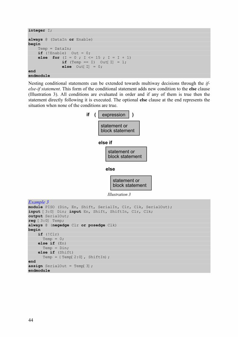
Nesting conditional statements can be extended towards multiway decisions through the if-else-if statement. This form of the conditional statement adds new condition to the else clause (Illustration 3). All conditions are evaluated in order and if any of them is true then the statement directly following it is executed. The optional else clause at the end represents the situation when none of the conditions are true.

if expression( )

else if

else

statement orblock statement

statement orblock statement

statement orblock statement

Illustration 3

Example 3 module PISO (Din, En, Shift, SerialIn, Clr, Clk, SerialOut); input [3:0] Din; input En, Shift, ShiftIn, Clr, Clk; output SerialOut; reg [3:0] Temp; always @ (negedge Clr or posedge Clk) begin

if (!Clr) Temp = 0; else if (En) Temp = Din; else if (Shift) Temp = {Temp[2:0], ShiftIn}; end

assign SerialOut = Temp[3]; endmodule

45

Initial Procedural Block

The initial procedural block is one of the forms of specifying behavior in Verilog (together with always procedural block, task, and function). Its specification consists of the initial keyword and the statement or block statement that will be executed when the procedural block is active (Illustration 1). The initial procedural block is activated at the beginning of a simulation and executes just once.

initial

begin

end

procedural statement

procedural statement

Illustration 1

The number of initial blocks in a single module is not limited and all blocks (both initial and always) are executed concurrently, without any predefined order.

Typically, initial blocks are used for initialization of values, clock generators and generating waveforms (Example 1).

Example 1 module TestVectors; reg [3:0] VectA, VectB; reg RegA, RegB, Clk; initial VectA = 4'b0000; // Single statement does not need to be grouped initial begin VectB = 4'bzzzz; // Multiple statements RegA = 1'bz; RegB = 1'bz; // need to be grouped #10 VectA = 4'b1010; #10 VectB = 4'b1111; #25 RegA = 1'b1; RegB = 1'b0; #5 VectB = 4'b0101; end initial // Clock generator begin Clk = 1'b0; forever #5 Clk = ~Clk; end initial #60 $finish; endmodule

46

Integer Data Type

integer is one of the register data types in Verilog HDL. An object is declared as integer using the integer keyword in the following way:

;,

integer register name ,

. . .

integer

integer register name

Illustration 1

Example 1 // Declaration of an integer register: integer Count;

The default initial value is zero.

Integer data objects are compatible with reg data objects and can be used exchangeable. The integer data type is introduced in the language for convenience of the user.

There is an important difference between integer and reg objects: integer values are stored as signed (in two's complement format), while reg values are always unsigned (Example 2). This has important consequence when arithmetic operation are used on such operands.

Example 2 reg [15:0]regA, regB; integer intA, intB; regA = -37; // In this case –37 will be represented // internally as 65499 intA = -37; // intA will be represented internally as -37 regB = 33; // This variable will be represented internally the same as intB = 33; // this one (33)

47

Integer Numbers

Integer numbers can be specified in decimal, hexadecimal, octal, or binary format. Decimal is default. Any integer number specified without a base is treated as an integer.

Example 1 // Legal numbers: 10 25 -12 -33 // Illegal numbers ('b' is not a decimal digit): -b1 1b0

If an integer number is specified in a non-decimal format, it requires a base format to be added (Illustration 1).

size numberbase format

Illustration 1

Base format is specified as a letter (case-insensitive) preceded by a single quote character ('). The letters used for that purpose are 'b' or 'B' for binary, 'd' or 'D' for decimal, 'h' or 'H' for hexadecimal and 'o' or 'O' for octal.

If a negative integer number is specified with a base, the unary minus sign must precede the complete number (i.e. the base). It cannot be specified between the base and the value.

Example 2 // Legal numbers: 8'b00011101 // the same as 8'B00011101 12'hafb // the same as 12'Hafb 15'h107d 15'o57340 -4'b0011 -8'hff 4'd12 -4'd11 // Illegal negative numbers: 2'b-11 4'd-12

Optionally, it can be specified with the size, which determines the number of bits for storing the number. If no size is specified, an implementation-dependent default size (at least 32 bits) is assumed:

Example 3 'd15 4'd12 -d'15 -4'd12 'hf0a7b 20'hf0a7b -'hf0a7b -20'hf0a7b 'o567 9'o567

48

When a unknown value ('x') or high impedance ('z') is used as one or more of the digits, it expands to one or more bits, depending on the base: it substitutes one bit for binary, three bits for octal and four bits for hexadecimal (Example).

Example 4 12'hazx // Equivalent to 1010zzzzxxxx 15'o56zzz // Equivalent to 101110zzzzzzzzz 16'h1xzz // Equivalent to 0001xxxxzzzzzzzz 12'o6zzz // Equivalent to 110zzzzzzzzz

If the number of digits specified is smaller than the size of the number, it is extended with the value of the leftmost digit if it is '0', 'x' or 'z' or with zeros if the leftmost digit is '1' (Example).

Example 5 8'bz110 // Equivalent to zzzzz110 12'oz34 // Equivalent to zzzzzz011100 10'hz1d // Equivalent to zz00011101 8'bx110 // Equivalent to xxxxx110 12'ox34 // Equivalent to xxxxxx011100 10'hx1d // Equivalent to xx00011101 8'b110 // Equivalent to 00000110 12'o134 // Equivalent to 000001011100 10'h11d // Equivalent to 0100011101 8'b010 // Equivalent to 00000010 12'o034 // Equivalent to 000000011100 10'h01d // Equivalent to 0000011101

Integer numbers may contain two special characters: an underscore ('_') and a question mark ('?'). An underscore has no meaning attached to it and its only purpose is to enhance readability. It can be inserted anywhere in the number except from the first character (Example 6).

Example 6 23_234_207 16'ha_b_1_0 8'b0001_1101

A question mark can be used as an alternative way of specifying the high-impedance value ('z') in numbers (Example 7).

Example 7 8'b?11?0? // Equivalent to zzz11z0z 15'o1?4? // Equivalent to 001zzz100zzz 12'hd1? // Equivalent to 11010001zzzz

49

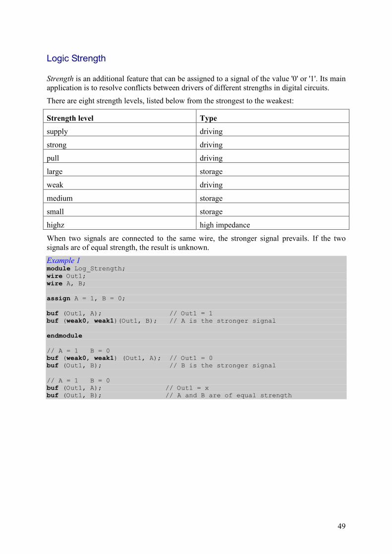
Logic Strength

Strength is an additional feature that can be assigned to a signal of the value '0' or '1'. Its main application is to resolve conflicts between drivers of different strengths in digital circuits.

There are eight strength levels, listed below from the strongest to the weakest:

Strength level Type

supply driving

strong driving

pull driving

large storage

weak driving

medium storage

small storage

highz high impedance

When two signals are connected to the same wire, the stronger signal prevails. If the two signals are of equal strength, the result is unknown.

Example 1 module Log_Strength; wire Out1; wire A, B; assign A = 1, B = 0; buf (Out1, A); // Out1 = 1 buf (weak0, weak1)(Out1, B); // A is the stronger signal endmodule

// A = 1 B = 0 buf (weak0, weak1) (Out1, A); // Out1 = 0 buf (Out1, B); // B is the stronger signal // A = 1 B = 0 buf (Out1, A); // Out1 = x buf (Out1, B); // A and B are of equal strength

50

Logic Values

Logical objects in Verilog can have any of the four values:

0 - logic zero or a false condition;

1 - logic one or a true condition;

x - unknown logic value;

z - high-impedance value.

The values 0 and 1 are logical complements of each other.

Unknown value and high-impedance can be written either in lower- and uppercase (x and z or X and Z, respectively).

Example 1 wire W1, W2; reg RegA, RegB; W1 = 1'b0; W2 = 1'b1; // Or W2 = 1 regA = 1'bz; // Or regA = 1'bZ regB = 1'bx; // Or regB = 1'bX

51

Logical Operators

There are three logical operators available:

&& logical and

|| logical or

! logical negation

Logical operations always evaluate to a single bit value: '0' (false), '1' (true) or 'x' (ambiguous).

If an operand is equal to zero, then it is a '0' (false) for a logical expression. A non-zero operand is treated as a logical '1' (true).

Example 1 reg [3:0] VectA, VectB; // VectA = 4'b1000 VectB = 4'b0 VectA && VectB // Evaluates to 0 VectA || VectB // Evaluates to 1 !VectA // Evaluates to 0 !VectB // Evaluates to 1 // VectA = 4'b1x00 VectB = 4'b1 VectA && VectB // Evaluates to x VectA || VectB // Evaluates to 1 !VectA // Evaluates to x !VectB // Evaluates to 0 integer A, B; (A==5) && (B==6) // This expression evaluates to 1 // if both A==5 and B==6 are true // and evaluates to 0 if either is false.

52

Module Definition

A module is the basic building block in Verilog (Illustration 1).

module

endmodule

declarations

concurrent statement

name of module ( ) ;list of ports

Illustration 1

A module definition begins with the module keyword and ends with the endmodule keyword.

The obligatory module name, and optional port list, port declarations and parameters must be specified as the first elements inside a module definition (Example 1).

Variable declarations, dataflow statements, instantiations of lower level modules, behavioral blocks, tasks and functions can be defined in any order and at any place inside a module definition (Example 2).

Example 1 module Full_Adder_with_varying_structure (A, B, Cin, Sum, Cout); parameter size=3; input [size-1:0] A,B; input Cin; output [size-1:0] Sum; output Cout; assign {Cout, Sum} = A + B + Cin; endmodule

Example 2 module TTL_74162 (EnT, EnP, Clear, Load, Clk, DataIn, DataOut, RCO); //==================// // Port declaration // //==================// input EnT, EnP; // EnT - enable T, EnP - Enable P input Clear, Load, Clk; input [3:0] DataIn; // Data inputs output [3:0] DataOut; // Data outputs output RCO; // RCO - Ripple Carry output //================================// // Temporary Register declaration // //================================// reg [3:0] DataOut; reg RCO; //==============// // Main process //

53

//==============// always @ (posedge Clk) begin casez ({Clear, Load, EnT, EnP}) 4'b0??? : begin DataOut = 4'b0; RCO = 1'b0; end 4'b10?? : begin DataOut = DataIn; RCO = 1'b0; end 4'b110? : begin DataOut = DataOut; RCO = 1'b0; end 4'b11?0 : begin DataOut = DataOut; RCO = 1'b0; end 4'b1111 : begin if (DataOut == 4'b1001) begin RCO = 1'b1; DataOut = 4'b0; end else begin DataOut = DataOut + 1; RCO = 1'b0; end end default : begin DataOut = 4'bxxxx; RCO = 1'bx; end endcase end endmodule

Modules cannot be nested, i.e. one module definition cannot contain another module definition between module and endmodule statements. It may, however, contain instances of other modules (Example 3).

Example 3 module Mux_2_to_1 (I0, I1, Sel, Y); //Port declarations: input I0, I1, Sel; // Input signals output Y; // Output signal wire S1, S2, S3; // Four instances of the module Nand nand gate1 (S1, Sel, Sel); nand gate2 (S2, S1, I0); nand gate3 (S3, Sel, I1); nand gate4 (Y, S2, S3); endmodule // Module definition

54

Module Instances

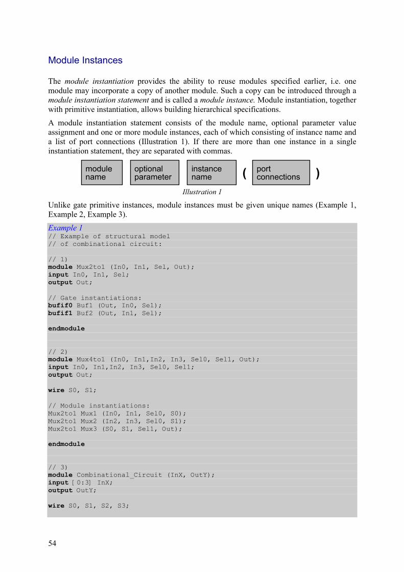
The module instantiation provides the ability to reuse modules specified earlier, i.e. one module may incorporate a copy of another module. Such a copy can be introduced through a module instantiation statement and is called a module instance. Module instantiation, together with primitive instantiation, allows building hierarchical specifications.

A module instantiation statement consists of the module name, optional parameter value assignment and one or more module instances, each of which consisting of instance name and a list of port connections (Illustration 1). If there are more than one instance in a single instantiation statement, they are separated with commas.

modulename

instancename

portconnections

optionalparameter ( )

Illustration 1

Unlike gate primitive instances, module instances must be given unique names (Example 1, Example 2, Example 3).

Example 1 // Example of structural model // of combinational circuit: // 1) module Mux2to1 (In0, In1, Sel, Out); input In0, In1, Sel; output Out; // Gate instantiations: bufif0 Buf1 (Out, In0, Sel); bufif1 Buf2 (Out, In1, Sel); endmodule

// 2) module Mux4to1 (In0, In1,In2, In3, Sel0, Sel1, Out); input In0, In1,In2, In3, Sel0, Sel1; output Out; wire S0, S1; // Module instantiations: Mux2to1 Mux1 (In0, In1, Sel0, S0); Mux2to1 Mux2 (In2, In3, Sel0, S1); Mux2to1 Mux3 (S0, S1, Sel1, Out); endmodule // 3) module Combinational_Circuit (InX, OutY); input [0:3] InX; output OutY; wire S0, S1, S2, S3;

55

// Gate instantiations: not NotGate (S0, InX[2]); xor XorGate (S1, InX[2], InX[3]); or OrGate (S2, InX[2], InX[3]); and AndGate (S3, InX[3], S0); // Module instantiation: Mux4to1 Mux (.In0(S1), .In1(S2), .In2(S3), .In3(InX[3]), .Sel0(InX[1]), .Sel1(InX[0]), .Out(OutY)); endmodule

Example 2 // Example of structural model // of 3-bit ripple asynchronous counter: // 1) module JK_MS (J, K, Clk, Clear, Q, Qbar); input J, K, Clk, Clear; output Q, Qbar; wire S1, S2, S3, S3bar, S4, S5, S6; nand Gate1 (S1, J, Clear, Clk, Qbar); nand Gate2 (S2, K, Clk, Q); nand Gate3 (S3, S1, S3bar); nand Gate4 (S3bar, S2, Clear, S3); nand Gate5 (S4, S6, S3); nand Gate6 (S5, S6, S3bar); nand Gate7 (Q, S4, Qbar); nand Gate8 (Qbar, S5, Clear, Q); nand Gate9 (S6, Clk); endmodule // 2) module RippleAsynCounter (Clock, Reset, Outputs); parameter One = 1'b1; input Clock, Reset; output [2:0] Outputs; JK_MS FF1 (.J(One), .K(One), .Clk(Clock), .Clear(Reset), .Q(Outputs[0]), .Qbar()); JK_MS FF2 (.K(One), .J(One), .Clear(Reset), .Clk(Outputs[0]), .Q(Outputs[1]), .Qbar()); JK_MS FF3 (.J(One), .K(One), .Clk(Outputs[1]), .Clear(Reset), .Q(Outputs[2]), .Qbar()); endmodule

Example 3 // Example of structural model // of 4-bit look-ahead synchronous counter: module Look_AheadSynCounter (Clock, Reset, Outputs);

56

parameter One = 1'b1, MSB = 4; input Clock, Reset; output [MSB-1:0] Outputs; wire Carry1, Carry2; JK_MS FF1 (One, One, Clock, Reset, Outputs[0], ); JK_MS FF2 (Outputs[0], Outputs[0], Clock, Reset, Outputs[1], ); and Gate1 (Carry1, Outputs[0], Outputs[1]); JK_MS FF3 (Carry1, Carry1, Clock, Reset, Outputs[2], ); and Gate2 (Carry2, Outputs[0], Outputs[1], Outputs[2]); JK_MS FF4 (Carry2, Carry2, Clock, Reset, Outputs[3], ); endmodule

57

Module Ports

Ports form an interface for a module, allowing it to communicate with its environment. The environment can communicate with a module only through its ports.

Ports are also called terminals.

Ports are specified only for those modules, which do communicate with the environment. An example of a module that does not communicate with the environment is a test bench.

The ports are listed in a port list of a module and declared fully in the port declaration inside the module. Both elements must be specified. The port list contains only the port names (Example 1).

Example 1 // Port list: module Counter (Clr, Clk, OE, Qout); . . . endmodule

All ports are of the type wire by default; therefore a port declaration contains only the type, determining the direction of the flow of data through each of them. There are three types of ports in Verilog HDL: input, output and bidirectional. They are declared using input, output, and inout keywords, respectively (Example 2).

Example 2 module Counter (Clr, Clk, OE, QOut); input Clr, OE, Clk; output [3:0] QOut; . . . endmodule

module RAM_Memory (CS, R_W, Addr, Data); input CS, R_W; input [15:0] Addr; inout [7:0] Data; . . . endmodule

The order of the port declarations need not be the same as the order of ports in the port list.

If an output port has to keep a value (i.e. it must be a registered output), this fact requires an additional declaration of the same port (Example 3). Only output ports can be registered.

Example 3 module Counter (Clr, Clk, OE, QOut); input Clr, OE, Clk; output [3:0] QOut; reg [3:0] Qout; . . . endmodule

module R0M_Memory (CS, OE, Addr, Data); input CS, OE; input [15:0] Addr; output [7:0] Data; reg [7:0] Data; . . . endmodule

58

Net Data Types

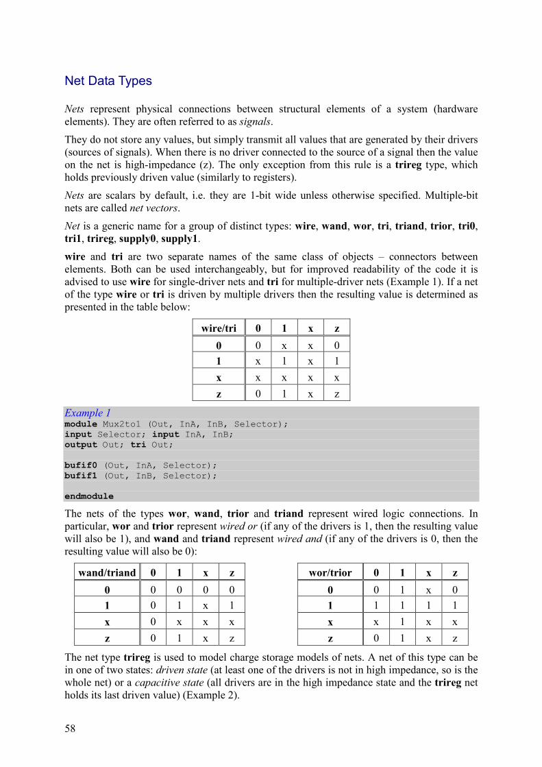
Nets represent physical connections between structural elements of a system (hardware elements). They are often referred to as signals.

They do not store any values, but simply transmit all values that are generated by their drivers (sources of signals). When there is no driver connected to the source of a signal then the value on the net is high-impedance (z). The only exception from this rule is a trireg type, which holds previously driven value (similarly to registers).

Nets are scalars by default, i.e. they are 1-bit wide unless otherwise specified. Multiple-bit nets are called net vectors.

Net is a generic name for a group of distinct types: wire, wand, wor, tri, triand, trior, tri0, tri1, trireg, supply0, supply1.

wire and tri are two separate names of the same class of objects – connectors between elements. Both can be used interchangeably, but for improved readability of the code it is advised to use wire for single-driver nets and tri for multiple-driver nets (Example 1). If a net of the type wire or tri is driven by multiple drivers then the resulting value is determined as presented in the table below:

wire/tri 0 1 x z

0 0 x x 0

1 x 1 x 1

x x x x x

z 0 1 x z

Example 1 module Mux2to1 (Out, InA, InB, Selector); input Selector; input InA, InB; output Out; tri Out; bufif0 (Out, InA, Selector); bufif1 (Out, InB, Selector); endmodule

The nets of the types wor, wand, trior and triand represent wired logic connections. In particular, wor and trior represent wired or (if any of the drivers is 1, then the resulting value will also be 1), and wand and triand represent wired and (if any of the drivers is 0, then the resulting value will also be 0):

wand/triand 0 1 x z wor/trior 0 1 x z

0 0 0 0 0 0 0 1 x 0

1 0 1 x 1 1 1 1 1 1

x 0 x x x x x 1 x x

z 0 1 x z z 0 1 x z

The net type trireg is used to model charge storage models of nets. A net of this type can be in one of two states: driven state (at least one of the drivers is not in high impedance, so is the whole net) or a capacitive state (all drivers are in the high impedance state and the trireg net holds its last driven value) (Example 2).

59

Example 2 module SimpleRegister (Out, A, Control); input A, Control; output Out; trireg Out; bufif1 (Out, A, Control); endmodule

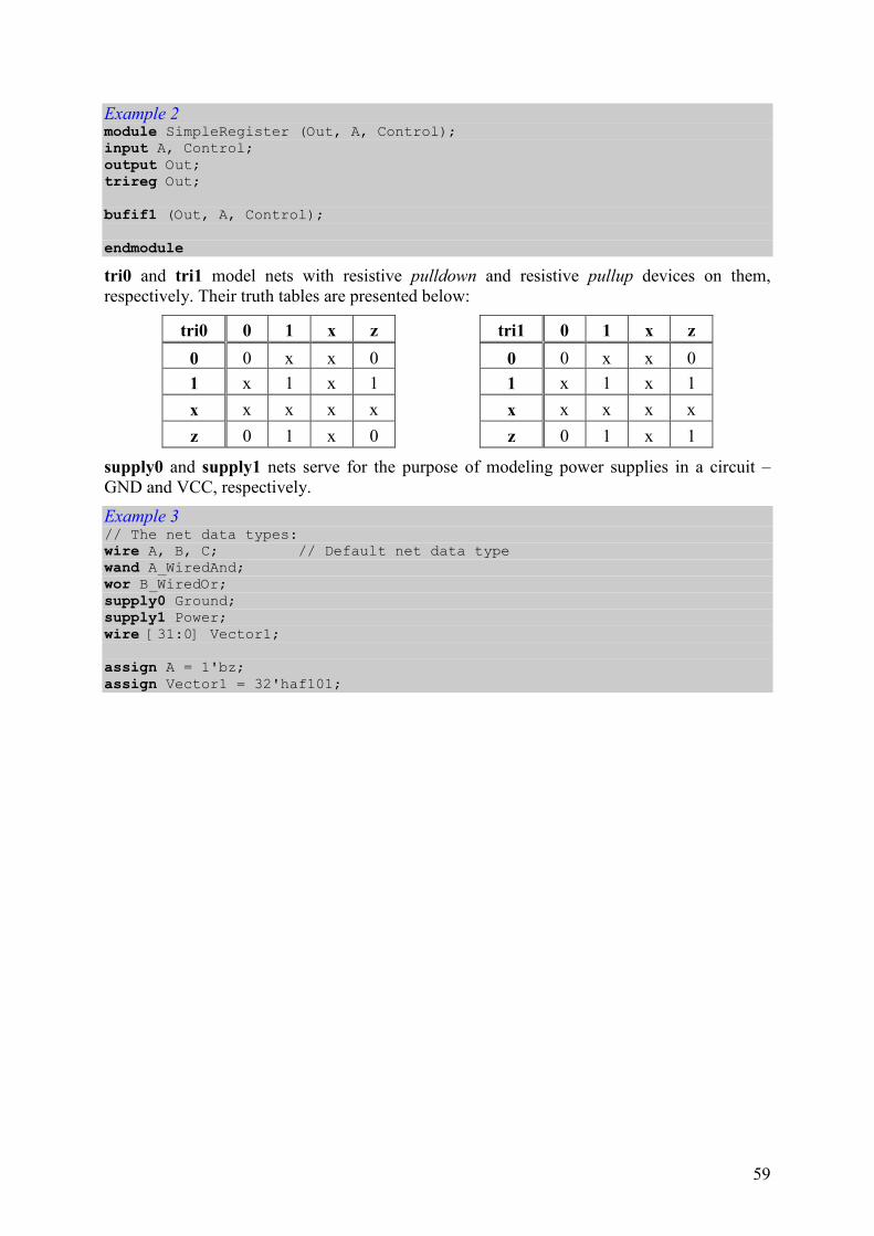
tri0 and tri1 model nets with resistive pulldown and resistive pullup devices on them, respectively. Their truth tables are presented below:

tri0 0 1 x z tri1 0 1 x z

0 0 x x 0 0 0 x x 0

1 x 1 x 1 1 x 1 x 1

x x x x x x x x x x

z 0 1 x 0 z 0 1 x 1

supply0 and supply1 nets serve for the purpose of modeling power supplies in a circuit – GND and VCC, respectively.

Example 3 // The net data types: wire A, B, C; // Default net data type wand A_WiredAnd; wor B_WiredOr; supply0 Ground; supply1 Power; wire [31:0] Vector1; assign A = 1'bz; assign Vector1 = 32'haf101;

60

Non-Blocking Assignment

See procedural assignment.

61

Number Representation

Numbers in Verilog HDL can be specified either as integer (Example 1) or real numbers (Example 2). In both cases there are different ways of representing the numbers – see Integer Numbers and Real Numbers for details.

Example 1 // Declaration of an integer registers: integer Int1, Int2; // Sized numbers: 5'b10011 // This is a 5-bit binary number 16'haafd // This is a 16-bit hexadecimal number 9'o234 // This is a 9-bit octal number 16'd255 // This is a 6-bit decimal number // Unsized numbers: 12345 // This is a 32-bit decimal number] 'haff // This is a 32-bit hexadecimal number 'o543 // This is a 32-bit octal number // Using underscore character in number: 33_345_112 12'b0011_1010_1101

Example 2 // Declaration of a real registers: real Real1, Real2; // Real numbers can be specified either in decimal // or in scientific notation // Decimal notation: 1.25 0.13 2345.254 // Scientific notation: 1.5E3 1.7e-4 23e2

62

Operators

Operators, together with operands form expressions. Operators define operations that are performed on operands in order to get new values for nets and registers.

Operators available in Verilog can be grouped according to the function they perform. The groups are listed below and each group is presented under a separate topic in this Reference Guide:

concatenation {}

arithmetic + - * / %

relational > >= < <=

logical ! && ||

equality == != === !==

bit-wise ~ & | ^ ^~ ~^

reduction & ~& | ~| ^ ^~ ~^

shift << >>

conditional ?:

If an expression contains more than one operator, then precedence rules for those operators apply. The rules determine which operators will be executed first:

unary + - ! ~ highest precedence (executed first)

* / %

binary + -

<< >>

< <= => >

== !== === !==

& ~&

^ ^~ ~^

| ~|

&&

||

?: lowest precedence

If two operators have the same precedence, they will be executed from left to right. If the order of execution based on precedence has to be changed, parentheses can be used for giving the highest precedence.

63

Parameters

Parameter is the Verilog's name for constant. Parameter objects are neither nets nor registers, as unlike the two their value cannot be changed during the runtime.

A parameter is declared with the parameter keyword (Example 1, Illustration 1):

name of parameter ,

;, . . .

parameter assignment=

name of parameter assignment=

Illustration 1

Example 1 parameter Size = 8;

Several parameters can be declared with a single parameter keyword. In such a case parameter commas separate declarations (Example 2):

Example 2 parameter DataSize = 8, BusSize = 16, MSB = 7, LSB = 0;

The value for a parameter must be a constant expression, i.e. it must be determinable at the compilation time.

The value of a parameter can be modified at compilation time with a defparam statement or in the module instance statement (Example 3).

Example 3 module Full_Adder (A, B, Cin, Sum, Cout); parameter Size=3; input [Size-1:0] A,B; input Cin; output [Size-1:0] Sum; output Cout; assign {Cout, Sum} = A + B + Cin; endmodule

module TopVer1; wire [7:0] A, B, Sum; wire Cin, Cout; // Use defparam statement defparam U1.Size = 8; // Instantiation of module Full_Adder Full_Adder U1 (A, B, Cin, Sum, Cout); endmodule

module TopVer2; wire [5:0] A, B, Sum; wire Cin, Cout;

64

// Instantiation of module Full_Adder with new Size value: Full_Adder #(6) U1 (A, B, Cin, Sum, Cout); endmodule

65

Part-Select

Part-select is a form of an expression operand allowing extracting several contiguous bits out of a vector (net or register). The selected sub-vector is determined by a range (Illustration 1). Each of the two indexes can be specified either as a constant value or a static expression (Example 1).

][ MSBvector name : LSB

Illustration 1

Example 1 wire [7:0] VectW; reg [0:5] VectR; // VectW = 8'b00111zx0; VectR = 6'bzzz01x; VectW[7:4] // Four most significant bits of vector 'VectW' // VectW[7:4] returns the bits 0011 VectR[3:5] // Three least significant bits of vector 'VectR' // VectR[3:5] returns the bits 01x VectW[2:2} // VectW[2:2] is the same as VectW[2] // and returns z

If any of the index values is unknown or high impedance, or the index falls out of the vector range, then the returned value will also be unknown (Example 2).

Example 2 wire [7:0] VectW; reg [0:5] VectR; VectW[5:7] // MSB and LSB of vector 'VectW' are reversed VectR[z:4] // Illegal non-constant expression

It is not allowed to specify part-select of a register declared as a real or realtime.

66

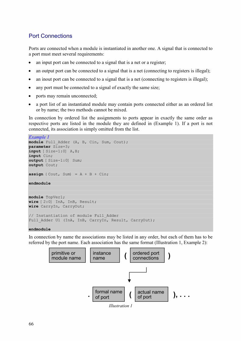
Port Connections

Ports are connected when a module is instantiated in another one. A signal that is connected to a port must meet several requirements:

• an input port can be connected to a signal that is a net or a register;

• an output port can be connected to a signal that is a net (connecting to registers is illegal);

• an inout port can be connected to a signal that is a net (connecting to registers is illegal);

• any port must be connected to a signal of exactly the same size;

• ports may remain unconnected;

• a port list of an instantiated module may contain ports connected either as an ordered list or by name; the two methods cannot be mixed.

In connection by ordered list the assignments to ports appear in exactly the same order as respective ports are listed in the module they are defined in (Example 1). If a port is not connected, its association is simply omitted from the list.

Example 1 module Full_Adder (A, B, Cin, Sum, Cout); parameter Size=3; input [Size-1:0] A,B; input Cin; output [Size-1:0] Sum; output Cout; assign {Cout, Sum} = A + B + Cin; endmodule

module TopVer1; wire [2:0] InA, InB, Result; wire CarryIn, CarryOut; // Instantiation of module Full_Adder Full_Adder U1 (InA, InB, CarryIn, Result, CarryOut); endmodule

In connection by name the associations may be listed in any order, but each of them has to be referred by the port name. Each association has the same format (Illustration 1, Example 2):

primitive ormodule name

instancename

formal nameof port

ordered portconnections( )

actual nameof port( ), . . ..

Illustration 1

67

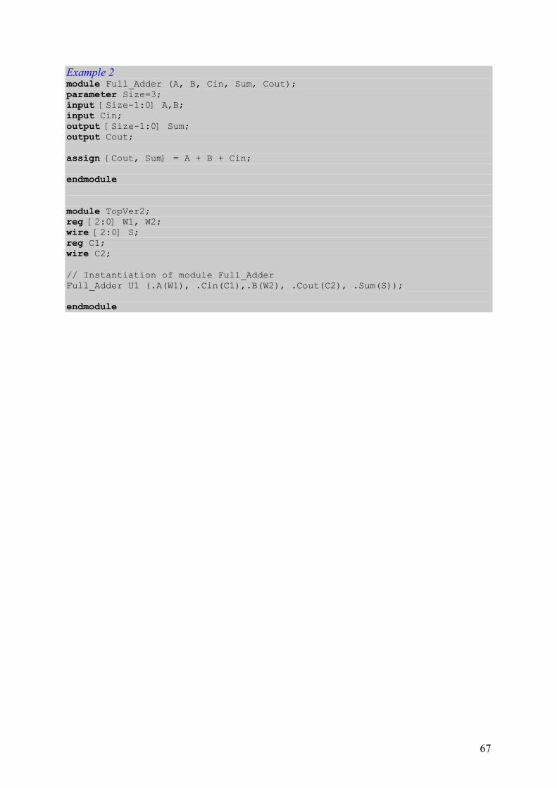
Example 2 module Full_Adder (A, B, Cin, Sum, Cout); parameter Size=3; input [Size-1:0] A,B; input Cin; output [Size-1:0] Sum; output Cout; assign {Cout, Sum} = A + B + Cin; endmodule

module TopVer2; reg [2:0] W1, W2; wire [2:0] S; reg C1; wire C2; // Instantiation of module Full_Adder Full_Adder U1 (.A(W1), .Cin(C1),.B(W2), .Cout(C2), .Sum(S)); endmodule

68

Primitives

Primitives are predefined Verilog modules specifying logical gates. They can be instantiated without the need for defining them again. Apart from predefined primitives Verilog HDL allows also using user-defined primitives (UDP). See respective topic for details.

There are three classes of logic primitives: and/or gates, buf/not gates and gates with control signal.

And/or gates have only one scalar (single bit) output and multiple scalar inputs. The first port on the port list denotes the output, while any subsequent ports determine the inputs (Example 1). This class contains six primitives: and, or, xor, nand, nor, and xnor. Their names are reserved keywords in Verilog HDL. Truth tables for two inputs for each of them are presented below:

and 0 1 x z or 0 1 x z xor 0 1 x z

0 0 0 0 0 0 0 1 x x 0 0 1 x x

1 0 1 x x 1 1 1 1 1 1 1 0 x x

x 0 x x x x x 1 x x x x x x x

z 0 x x x z x 1 x x z x x x x

nand 0 1 x z nor 0 1 x z xnor 0 1 x z

0 1 1 1 1 0 1 0 x x 0 1 0 x x

1 1 0 x x 1 0 0 0 0 1 0 1 x x

x 1 x x x x x 0 x x x x x x x

z 1 x x x z x 0 x x z x x x x

Example 1 wire Out1, Out2, Out3, Out4; wire In1, In2, In3; reg In4; and (Out1, In2, In2, In3); or (Out2, In2, In3); nand (Out3, In2, In2, In3); xor (Out4, In2, In3, In4);

Buf/not gates have one scalar input and one or more scalar outputs. The last port on the port list denotes the input, while any preceding ports determine the outputs (Example 2). This class contains two primitives: buf and not. Their names are reserved words in Verilog HDL. Truth tables for a single output for each of them are presented below:

buf not

input output input output

0 0 0 1

1 1 1 0

x x x x

z x z x

Example 2

69

wire Out1, Out2, Out3, Out4, Out5, Out6; wire In1, In2, In3, In4; buf (Out1, In1); buf (Out2, Out3,In2); not (Out4, In3); not (Out5, Out6, In4);

Gates with control signal are the Verilog way of specifying three-state buffers with or without inversion. This class contains four primitives: bufif0, bufif1, notif0, and notif1. The digit at the end of the name of the primitive (each of which is a reserved keyword) denotes the logical value of the control signal assertion. If the control signal is deasserted, the output will be set to high-impedance value as shown in the truth tables below.

CONTROL CONTROL bufif0

0 1 x z bufif1

0 1 x z

D 0 0 z L L D 0 z 0 L L

A 1 1 z H H A 1 z 1 H H

T x x z x x T x z x x x

A z x z x x A z z x x x

CONTROL CONTROL notif0

0 1 x z notif1

0 1 x z

D 0 1 z H H D 0 z 1 H H

A 1 0 z L L A 1 z 0 L L

T x x z x x T x z x x x

A z x z x x A z z x x x

Each gate with control signal has exactly three ports. The first port is the output, the second is the input and the third is the control signal (Illustration 1 and Example 3).

Control

InA OutA

bufif0 bufif1

notif0 notif1

(OutA, InA, Control) (OutB, InB, Control)

(OutC, InC, Control) (OutD, InD, Control)

Control

Control Control

OutB

OutC OutD

InB

InC InD

Illustration 1

Example 3 wire Out1, Out2, Out3, Out4; wire In1, In2; wire Control1, Control2; bufif1 (Out1, In1, Control1);

70

bufif0 (Out2, In2, Control2); notif1 (Out3, In1, Control1); notif0 (Out4, In2, Control2);

71

Primitive Instances

The primitive instantiation is a mechanism for using predefined primitives – gates or switches – in a Verilog structural specification. Each primitive instance represents a single gate and consists of the following elements (Illustration 1):

primitivename

optionalinstance name

portconnections

optionalparameter ( )

Illustration 1

- The keyword denoting the gate or switch type - An optional drive strength - An optional propagation delay - An optional identifier of the instance - An optional range for array of instances - The terminal connection list.

In its minimal form, a primitive instantiation contains only the gate type keyword and the terminal connection list (Example 1).

Example 1 module OneBitFullAdder_ver1 (A, B, Cin, Sum, Cout); input A, B, Cin; output Sum, Cout; // Internal wire declarations: wire AxorB, AandCin, BandCin, AandB; // Gate instantiations without instance name: xor (AxorB, A, B); xor (Sum, AxorB, Cin); and (AandCin, A, Cin); and (BandCin, B, Cin); and (AandB, A, B); or (Cout, AandCin, BandCin, AandB); endmodule

Often two optional elements are added to a primitive instance: a propagation delay and an identifier (Example 2).

Example 2 module Mux2to1_ver1 (In0, In1, Sel, Out); input In0, In1, Sel; output Out; // Internal wire declarations: wire NotSel, S1, S2; // Gate instantiations: not #5 Gate1 (NotSel, Sel); and #6 Gate2 (S1, NotSel, In0); and #6 Gate3 (S2, Sel, In1); or #7 Gate4 (Out, S1, S2); endmodule

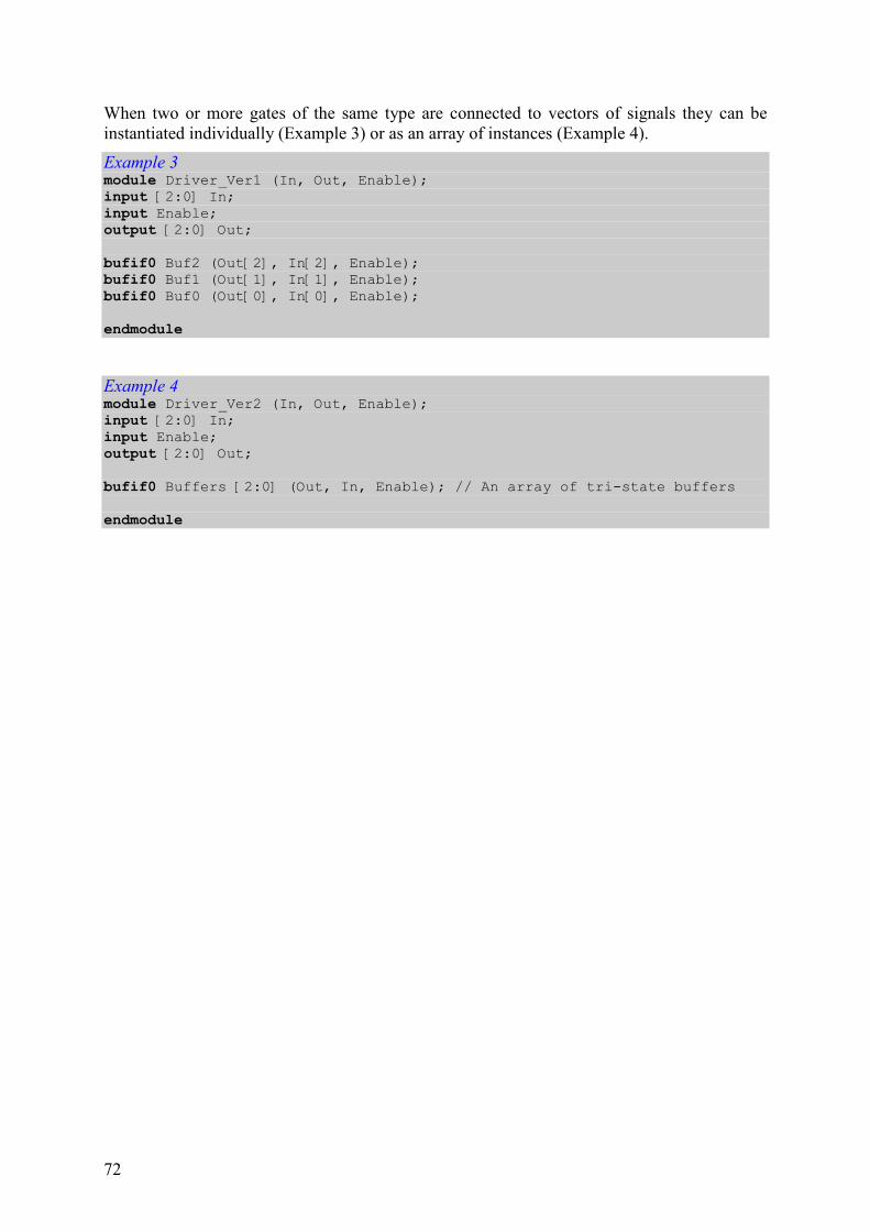
72

When two or more gates of the same type are connected to vectors of signals they can be instantiated individually (Example 3) or as an array of instances (Example 4).

Example 3 module Driver_Ver1 (In, Out, Enable); input [2:0] In; input Enable; output [2:0] Out; bufif0 Buf2 (Out[2], In[2], Enable); bufif0 Buf1 (Out[1], In[1], Enable); bufif0 Buf0 (Out[0], In[0], Enable); endmodule

Example 4 module Driver_Ver2 (In, Out, Enable); input [2:0] In; input Enable; output [2:0] Out; bufif0 Buffers [2:0] (Out, In, Enable); // An array of tri-state buffers endmodule

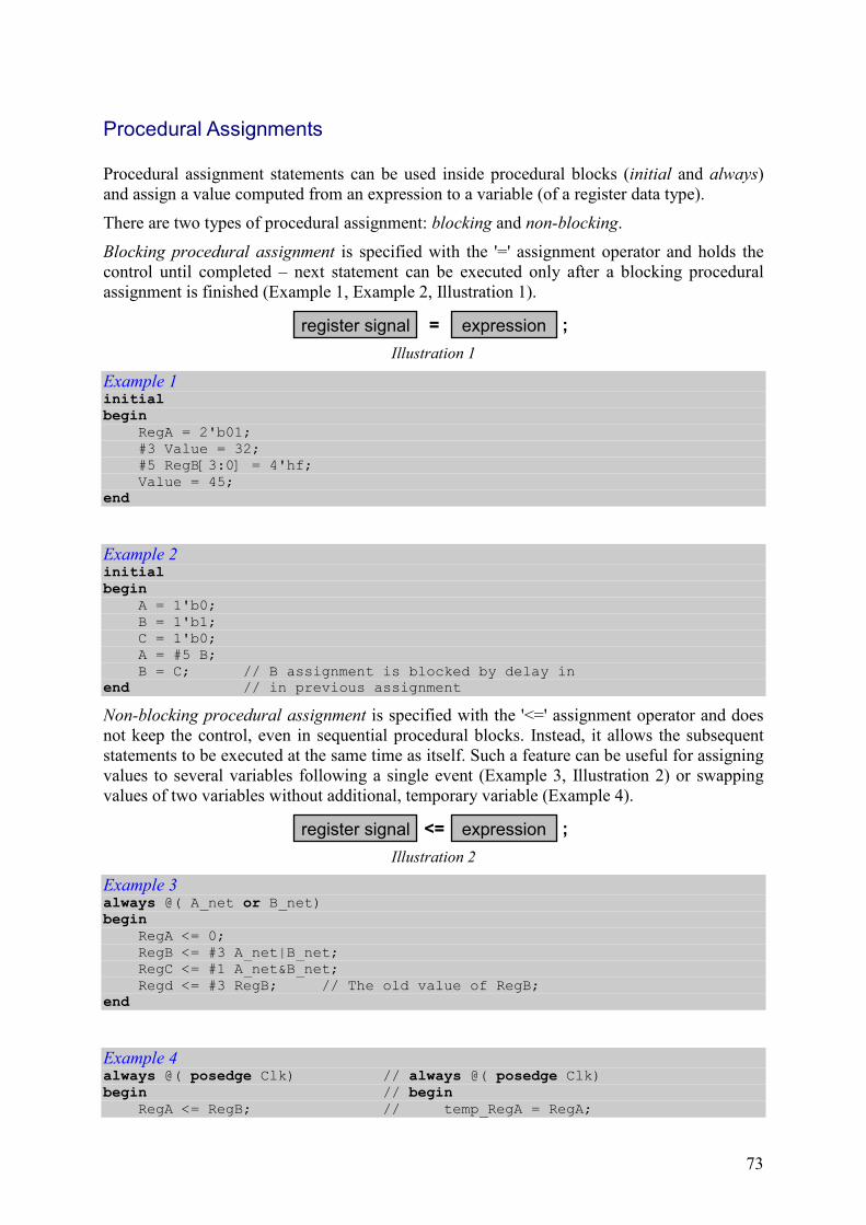
73

Procedural Assignments

Procedural assignment statements can be used inside procedural blocks (initial and always) and assign a value computed from an expression to a variable (of a register data type).

There are two types of procedural assignment: blocking and non-blocking.

Blocking procedural assignment is specified with the '=' assignment operator and holds the control until completed – next statement can be executed only after a blocking procedural assignment is finished (Example 1, Example 2, Illustration 1).

= expressionregister signal ;

Illustration 1

Example 1 initial begin RegA = 2'b01; #3 Value = 32; #5 RegB[3:0] = 4'hf; Value = 45; end

Example 2 initial begin A = 1'b0; B = 1'b1; C = 1'b0; A = #5 B; B = C; // B assignment is blocked by delay in end // in previous assignment

Non-blocking procedural assignment is specified with the '<=' assignment operator and does not keep the control, even in sequential procedural blocks. Instead, it allows the subsequent statements to be executed at the same time as itself. Such a feature can be useful for assigning values to several variables following a single event (Example 3, Illustration 2) or swapping values of two variables without additional, temporary variable (Example 4).

<= expressionregister signal ;

Illustration 2

Example 3 always @( A_net or B_net) begin

RegA <= 0; RegB <= #3 A_net|B_net; RegC <= #1 A_net&B_net; Regd <= #3 RegB; // The old value of RegB; end

Example 4 always @( posedge Clk) // always @( posedge Clk) begin // begin RegA <= RegB; // temp_RegA = RegA;

74

RegB <= RegA; // temp_RegB = RegB; end // RegA = temp_RegB; // RegA = temp_RegB; // end

75

Procedural Blocks

Procedural blocks (initial and always) (Example 1) are the two basic statements in behavioral modeling. All behavioral statements can appear only inside these blocks (Example 2).

Example 1 module Clock_Generator; parameter Half_Cycle = 10; reg Clk; initial Clk = 1'b0; // Initialize Clk at time 0 always #Half_Cycle Clk = ~Clk; // Toggle Clk every Half_Cycle endmodule

Example 2 module JK_NegEdgeFlip_Flop (Q, Qbar, J, K, Clk); input J, K, Clk; output Q, Qbar; reg Q, Qbar; reg J, K; always @ (negedge Clk or J or K) begin if ((J==0)&&(K==1)) begin Q=0; Qbar=1; end else if ((J==1)&&(K==0)) begin Q=0; Qbar=1; end else if ((J==0)&&(K==0)) begin Q=Q; Qbar=Qbar; end else ((J==1)&&(K==1)) begin Q=QBar; Qbar=Q; end end endmodule

Procedural blocks represent separate activity flows. Each activity flow can be either sequential (Example 3) or concurrent (Example 4).

Example 3 module Sequential_Blocks;

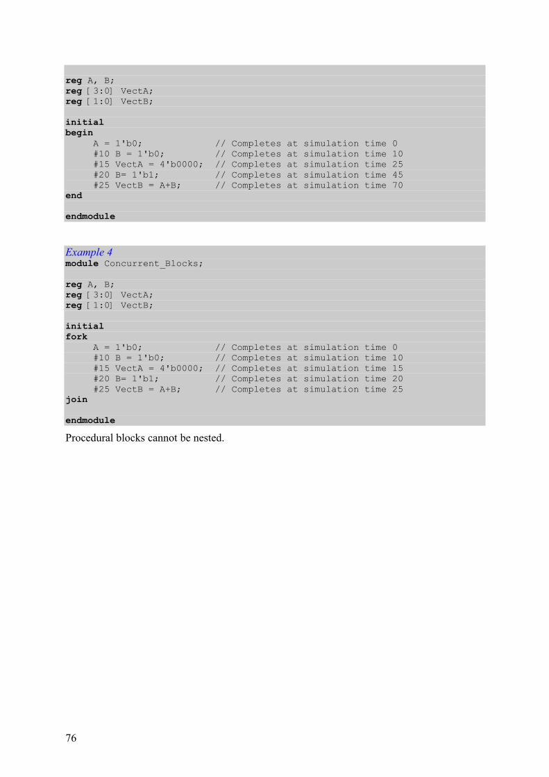
76

reg A, B; reg [3:0] VectA; reg [1:0] VectB; initial begin A = 1'b0; // Completes at simulation time 0 #10 B = 1'b0; // Completes at simulation time 10 #15 VectA = 4'b0000; // Completes at simulation time 25 #20 B= 1'b1; // Completes at simulation time 45 #25 VectB = A+B; // Completes at simulation time 70 end endmodule

Example 4 module Concurrent_Blocks; reg A, B; reg [3:0] VectA; reg [1:0] VectB; initial fork A = 1'b0; // Completes at simulation time 0 #10 B = 1'b0; // Completes at simulation time 10 #15 VectA = 4'b0000; // Completes at simulation time 15 #20 B= 1'b1; // Completes at simulation time 20 #25 VectB = A+B; // Completes at simulation time 25 join endmodule

Procedural blocks cannot be nested.

77

Real Data Type

real is one of the register data types in Verilog HDL.

An object is declared as real using the real keyword in the following way (Illustration 1, Example 1):

;,

real register name ,

. . .

real

real register name

Illustration 1

Example 1 // Declaration of a real register: real AverVal;

The default initial value is zero.

Not all Verilog operators can be used on real operands (registers or numbers). Expressions containing real operands may contain the following operators:

• unary '+' and '-';

• arithmetic '+', '-', '*' and '/';

• relational '>', '>=', '<', and '<=';

• logical '!', '&&', and '||';

• logical equality '==' and '!=';

• conditional '?:;'

• event or 'or'.

It is not allowed to use the following operators in real expressions:

• concatenation and replication '{}', '{{}}';

• modulus '%';

• case equality '===', and '!==';

• bit-wise logical operators '~', '&', '|', '^', '^~', and '~^';

• reduction operators '^', '^~', '~^', '&', '~&', '|', and '~|';

• shift operators '<<' and '>>'

It is not allowed to declare arrays of real registers.

78

Real Numbers

Real numbers can be specified either in decimal notation or in scientific notation. Underscore character ('_') can be used to improve readability. All underscores inside numbers are ignored.

When decimal notation is used at least one digit must be specified on each side of the decimal point (Example 1).

Example 1 // Correct real numbers: 1.5 0.2143 5.0 // Incorrect real numbers: .2143 5.

The exponent symbol used in scientific notation can be written either as 'e' or 'E', i.e. in lower- or uppercase (Example 2).

Example 2 // Correct real numbers: 1.5e2 3E-2 5.0e10 // Incorrect real numbers: .2143e3 5.e10

When a real number is assigned to an integer variable, it is implicitly converted by rounding to the nearest integer away from zero (Example 3).

Example 3 -26.2 will be converted to –27 26.2 will be converted to 26 -13.5 will be converted to –14 13.5 will be converted to 14

79

Reduction Operators

Reduction operators are unary, i.e. they operate on a single operand (Illustration 1). The single-bit result is determined according to the operator: in case of reduction and, reduction or and reduction xor respective logical operation is applied to the first and second bit, then to the result of this and third bit, etc. In case of reduction nand, reduction nor and reduction xnor the result is computed as an inversion of reduction and, reduction or and reduction xor, respectively.

reduction operator single operand

Illustration 1

The results of applying reduction operators to pairs of bit values are the same as in bit-wise operators and are presented below:

reduction

and

reduction

or

reduction

xor operands

& | ^

0 0 0 0 0

0 1 0 1 1

0 x 0 x x

0 z 0 x x

1 0 1 1 1

1 1 1 1 0

1 x x 1 x

1 z x 1 x

x 0 0 x x

x 1 x 1 x

x x x x x

x z x x x

z 0 0 x x

z 1 x 1 x

z x x x x

z z x x x

Example 1:

Example 1 reg [3:0] VectA, VectB, VectC, VectD; // VectA = 4'b0000 VectB = 4'b1111 VectC = 4'b0101 VectD = 4'b0111 // 1) Reduction and

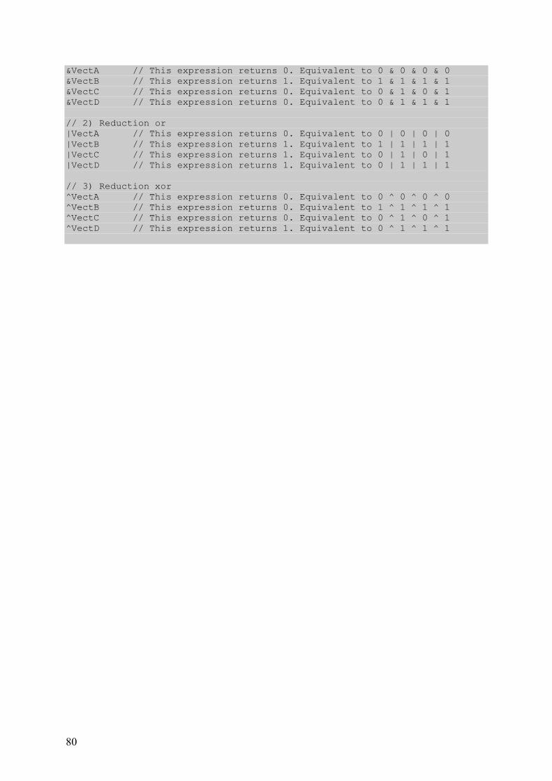
80

&VectA // This expression returns 0. Equivalent to 0 & 0 & 0 & 0 &VectB // This expression returns 1. Equivalent to 1 & 1 & 1 & 1 &VectC // This expression returns 0. Equivalent to 0 & 1 & 0 & 1 &VectD // This expression returns 0. Equivalent to 0 & 1 & 1 & 1 // 2) Reduction or |VectA // This expression returns 0. Equivalent to 0 | 0 | 0 | 0 |VectB // This expression returns 1. Equivalent to 1 | 1 | 1 | 1 |VectC // This expression returns 1. Equivalent to 0 | 1 | 0 | 1 |VectD // This expression returns 1. Equivalent to 0 | 1 | 1 | 1 // 3) Reduction xor ^VectA // This expression returns 0. Equivalent to 0 ^ 0 ^ 0 ^ 0 ^VectB // This expression returns 0. Equivalent to 1 ^ 1 ^ 1 ^ 1 ^VectC // This expression returns 0. Equivalent to 0 ^ 1 ^ 0 ^ 1 ^VectD // This expression returns 1. Equivalent to 0 ^ 1 ^ 1 ^ 1

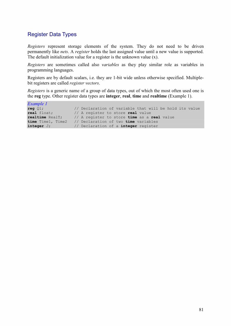
81

Register Data Types

Registers represent storage elements of the system. They do not need to be driven permanently like nets. A register holds the last assigned value until a new value is supported. The default initialization value for a register is the unknown value (x).

Registers are sometimes called also variables as they play similar role as variables in programming languages.

Registers are by default scalars, i.e. they are 1-bit wide unless otherwise specified. Multiple-bit registers are called register vectors.

Registers is a generic name of a group of data types, out of which the most often used one is the reg type. Other register data types are integer, real, time and realtime (Example 1).

Example 1 reg Q1; // Declaration of variable that will be hold its value real float; // A register to store real value realtime RealT; // A register to store time as a real value time Time1, Time2 // Declaration of two time variables integer J; // Declaration of a integer register

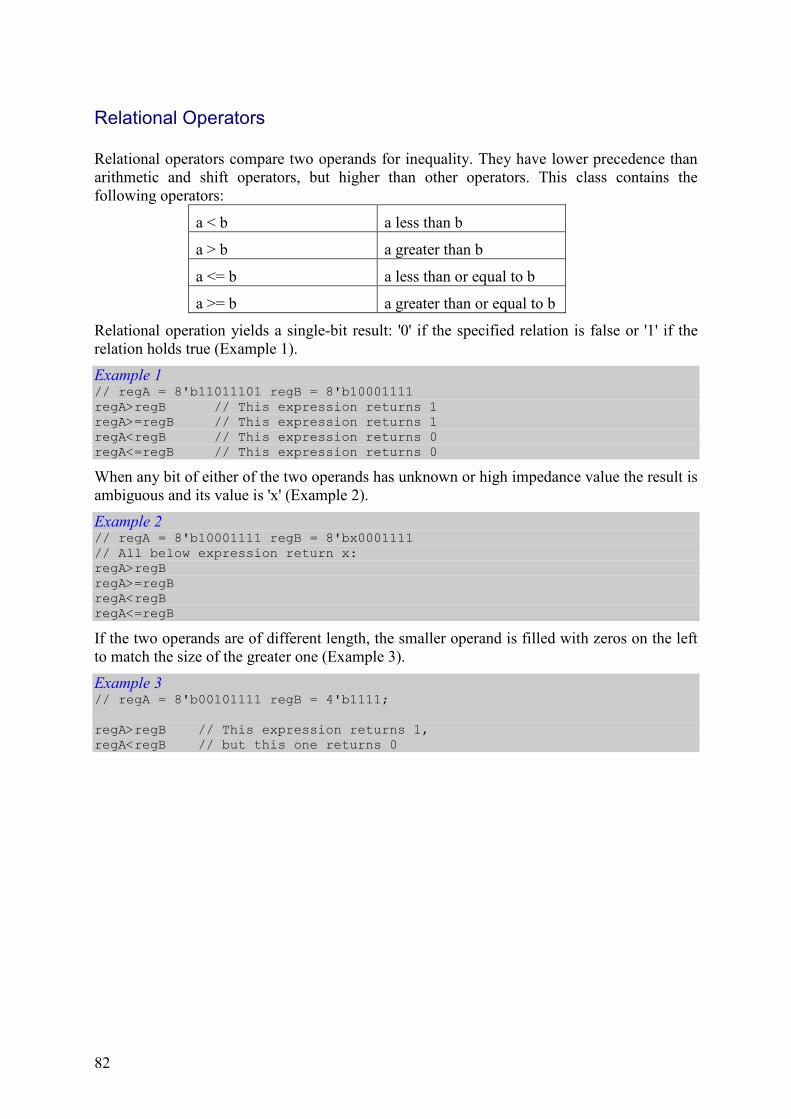
82

Relational Operators

Relational operators compare two operands for inequality. They have lower precedence than arithmetic and shift operators, but higher than other operators. This class contains the following operators:

a < b a less than b

a > b a greater than b

a <= b a less than or equal to b

a >= b a greater than or equal to b

Relational operation yields a single-bit result: '0' if the specified relation is false or '1' if the relation holds true (Example 1).

Example 1 // regA = 8'b11011101 regB = 8'b10001111 regA>regB // This expression returns 1 regA>=regB // This expression returns 1 regA<regB // This expression returns 0 regA<=regB // This expression returns 0

When any bit of either of the two operands has unknown or high impedance value the result is ambiguous and its value is 'x' (Example 2).

Example 2 // regA = 8'b10001111 regB = 8'bx0001111 // All below expression return x: regA>regB regA>=regB regA<regB regA<=regB

If the two operands are of different length, the smaller operand is filled with zeros on the left to match the size of the greater one (Example 3).

Example 3 // regA = 8'b00101111 regB = 4'b1111; regA>regB // This expression returns 1, regA<regB // but this one returns 0

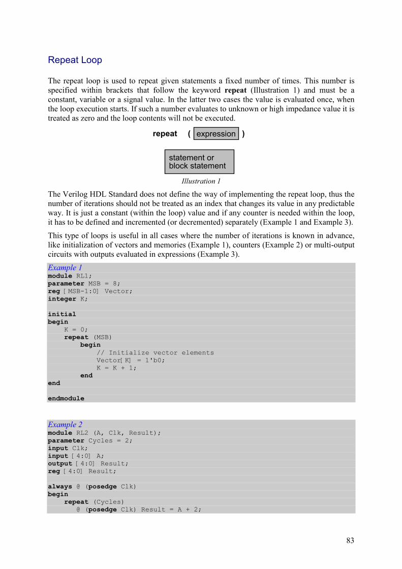
83

Repeat Loop

The repeat loop is used to repeat given statements a fixed number of times. This number is specified within brackets that follow the keyword repeat (Illustration 1) and must be a constant, variable or a signal value. In the latter two cases the value is evaluated once, when the loop execution starts. If such a number evaluates to unknown or high impedance value it is treated as zero and the loop contents will not be executed.

statement orblock statement

repeat expression( )

Illustration 1

The Verilog HDL Standard does not define the way of implementing the repeat loop, thus the number of iterations should not be treated as an index that changes its value in any predictable way. It is just a constant (within the loop) value and if any counter is needed within the loop, it has to be defined and incremented (or decremented) separately (Example 1 and Example 3).

This type of loops is useful in all cases where the number of iterations is known in advance, like initialization of vectors and memories (Example 1), counters (Example 2) or multi-output circuits with outputs evaluated in expressions (Example 3).

Example 1 module RL1; parameter MSB = 8; reg [MSB-1:0] Vector; integer K; initial begin

K = 0; repeat (MSB) begin // Initialize vector elements Vector[K] = 1'b0; K = K + 1; end end endmodule

Example 2 module RL2 (A, Clk, Result); parameter Cycles = 2; input Clk; input [4:0] A; output [4:0] Result; reg [4:0] Result; always @ (posedge Clk) begin

repeat (Cycles) @ (posedge Clk) Result = A + 2;

84

end endmodule

Example 3 module Decoder (D, En, Out); input [3:0] D; input En; output [15:0] Out; reg [15:0] Out; reg [3:0] Temp; integer I; always @ (D or En) begin

I = 16; Temp = D; if (!En) Out = 0; else repeat (15) begin if (Temp == I-1) Out[I-1] = 1; else Out[I-1] = 0; I = I-1; end end

endmodule

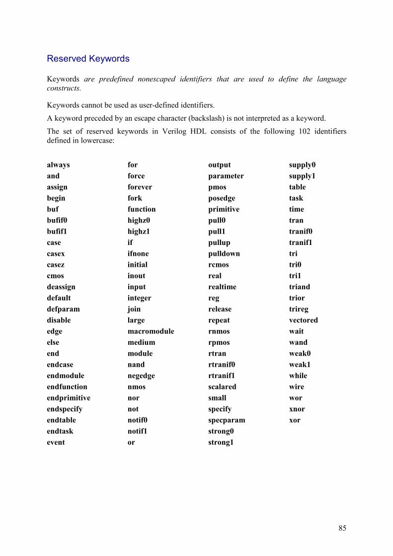
85

Reserved Keywords

Keywords are predefined nonescaped identifiers that are used to define the language constructs.

Keywords cannot be used as user-defined identifiers.

A keyword preceded by an escape character (backslash) is not interpreted as a keyword.

The set of reserved keywords in Verilog HDL consists of the following 102 identifiers defined in lowercase:

always

and

assign

begin

buf

bufif0

bufif1

case

casex

casez

cmos

deassign

default

defparam

disable

edge

else

end

endcase

endmodule

endfunction

endprimitive

endspecify

endtable

endtask

event

for

force

forever

fork

function

highz0

highz1

if

ifnone

initial

inout

input

integer

join

large

macromodule

medium

module

nand

negedge

nmos

nor

not

notif0

notif1

or

output

parameter

pmos

posedge

primitive

pull0

pull1

pullup

pulldown

rcmos

real

realtime

reg

release

repeat

rnmos

rpmos

rtran

rtranif0

rtranif1

scalared

small

specify

specparam

strong0

strong1

supply0

supply1

table

task

time

tran

tranif0

tranif1

tri

tri0

tri1

triand

trior

trireg

vectored

wait

wand

weak0

weak1

while

wire

wor

xnor

xor

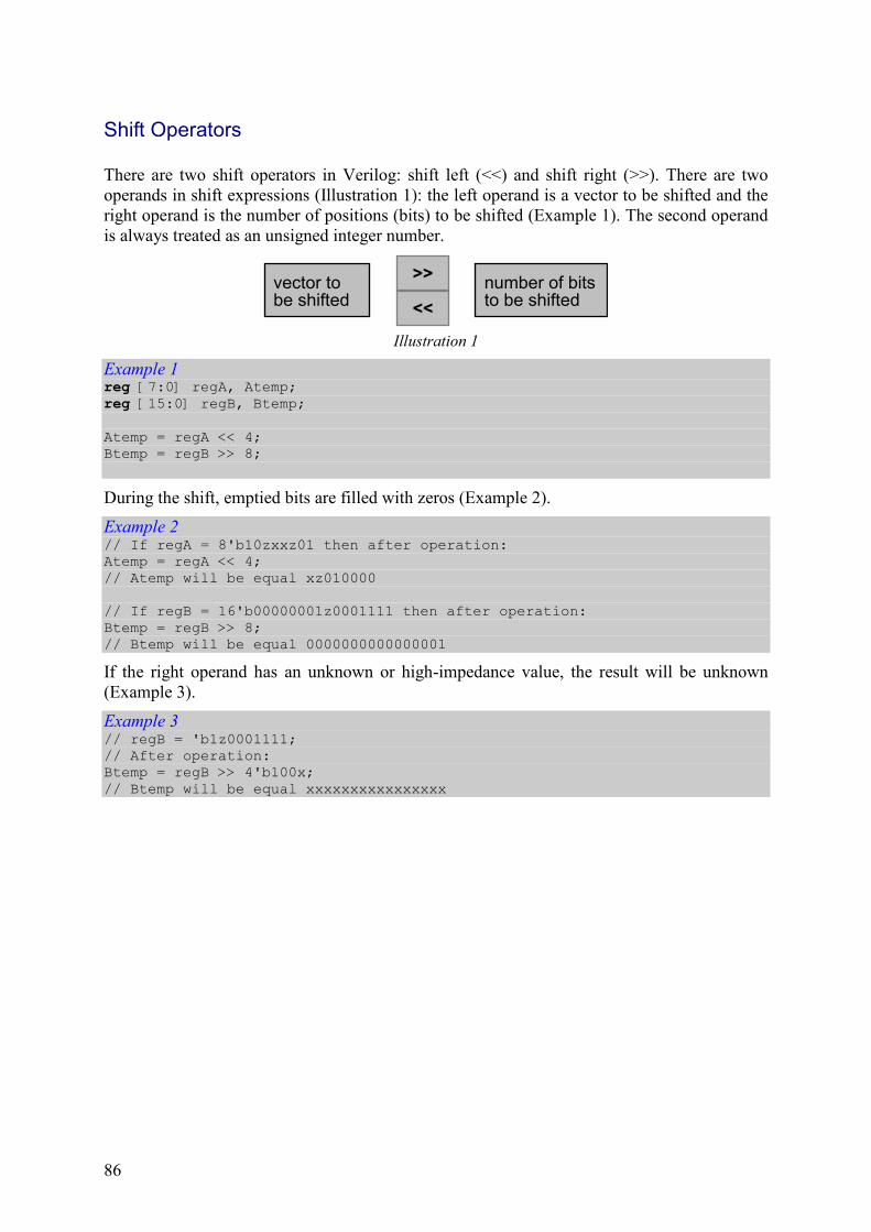
86

Shift Operators

There are two shift operators in Verilog: shift left (<<) and shift right (>>). There are two operands in shift expressions (Illustration 1): the left operand is a vector to be shifted and the right operand is the number of positions (bits) to be shifted (Example 1). The second operand is always treated as an unsigned integer number.

vector tobe shifted

number of bitsto be shifted<<

>>

Illustration 1

Example 1 reg [7:0] regA, Atemp; reg [15:0] regB, Btemp; Atemp = regA << 4; Btemp = regB >> 8;

During the shift, emptied bits are filled with zeros (Example 2).

Example 2 // If regA = 8'b10zxxz01 then after operation: Atemp = regA << 4; // Atemp will be equal xz010000 // If regB = 16'b00000001z0001111 then after operation: Btemp = regB >> 8; // Btemp will be equal 0000000000000001

If the right operand has an unknown or high-impedance value, the result will be unknown (Example 3).

Example 3 // regB = 'b1z0001111; // After operation: Btemp = regB >> 4'b100x; // Btemp will be equal xxxxxxxxxxxxxxxx

87

String Data Type

A string is a sequence of characters enclosed by double quotes. A string must fit in a single line (Illustration 1).

number of char. * 8reg [ : 1 ] string name

Illustration 1

String variables are declared as register vectors, where the width of the vector equals to the number of characters in the string multiplied by eight (Example 1).

Example 1 // A variable to store the string "Evita" should be declared as: reg [40:1] EvitaStr; // 5 characters * 8 // and the string could be assigned as: initial

begin EvitaStr = "Evita"; end

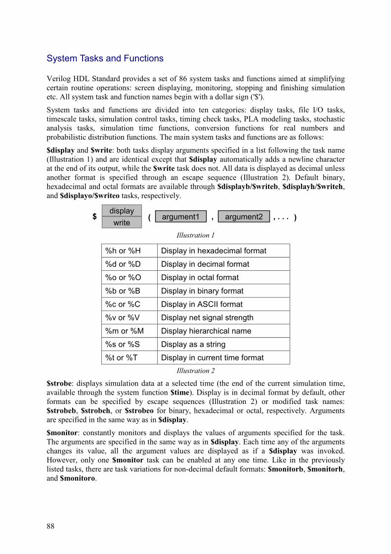
88

System Tasks and Functions

Verilog HDL Standard provides a set of 86 system tasks and functions aimed at simplifying certain routine operations: screen displaying, monitoring, stopping and finishing simulation etc. All system task and function names begin with a dollar sign ('$').

System tasks and functions are divided into ten categories: display tasks, file I/O tasks, timescale tasks, simulation control tasks, timing check tasks, PLA modeling tasks, stochastic analysis tasks, simulation time functions, conversion functions for real numbers and probabilistic distribution functions. The main system tasks and functions are as follows:

$display and $write: both tasks display arguments specified in a list following the task name (Illustration 1) and are identical except that $display automatically adds a newline character at the end of its output, while the $write task does not. All data is displayed as decimal unless another format is specified through an escape sequence (Illustration 2). Default binary, hexadecimal and octal formats are available through $displayb/$writeb, $displayh/$writeh, and $displayo/$writeo tasks, respectively.

write

display$ ( )argument1 argument2, , . . .

Illustration 1

%h or %H Display in hexadecimal format

%d or %D Display in decimal format

%o or %O Display in octal format

%b or %B Display in binary format

%c or %C Display in ASCII format

%v or %V Display net signal strength

%m or %M Display hierarchical name

%s or %S Display as a string

%t or %T Display in current time format

Illustration 2

$strobe: displays simulation data at a selected time (the end of the current simulation time, available through the system function $time). Display is in decimal format by default, other formats can be specified by escape sequences (Illustration 2) or modified task names: $strobeb, $strobeh, or $strobeo for binary, hexadecimal or octal, respectively. Arguments are specified in the same way as in $display.

$monitor: constantly monitors and displays the values of arguments specified for the task. The arguments are specified in the same way as in $display. Each time any of the arguments changes its value, all the argument values are displayed as if a $display was invoked. However, only one $monitor task can be enabled at any one time. Like in the previously listed tasks, there are task variations for non-decimal default formats: $monitorb, $monitorh, and $monitoro.

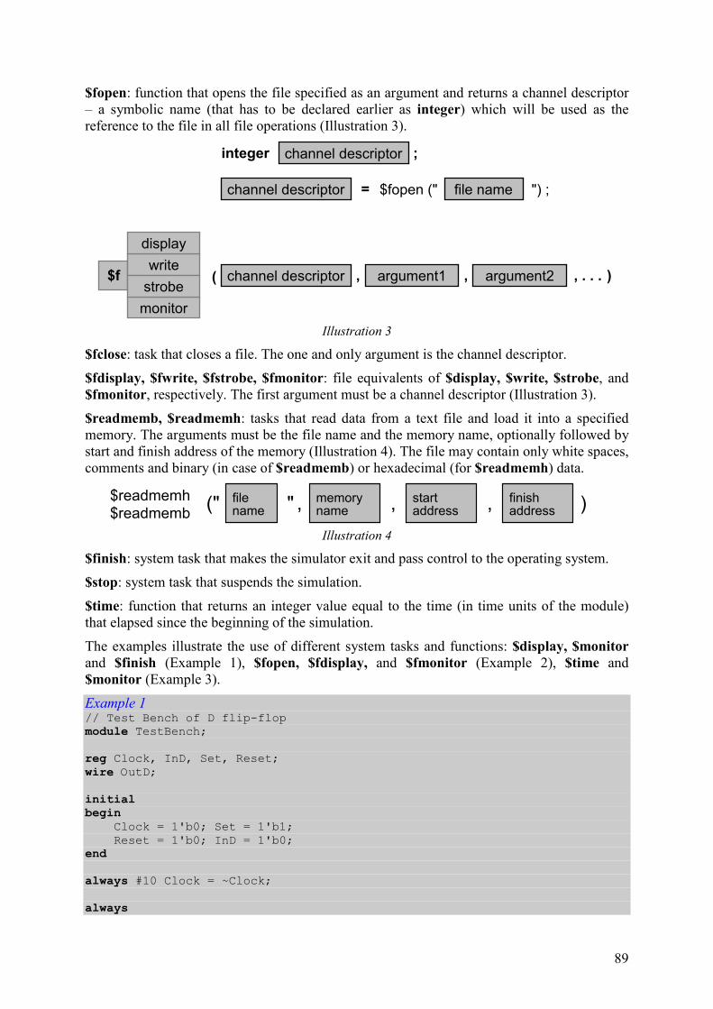
89

$fopen: function that opens the file specified as an argument and returns a channel descriptor – a symbolic name (that has to be declared earlier as integer) which will be used as the reference to the file in all file operations (Illustration 3).

write

display

$f ( )channel descriptor argument1, , . . .argument2,

monitor

strobe

integer channel descriptor ;

channel descriptor = $fopen (" file name ") ;

Illustration 3

$fclose: task that closes a file. The one and only argument is the channel descriptor.

$fdisplay, $fwrite, $fstrobe, $fmonitor: file equivalents of $display, $write, $strobe, and $fmonitor, respectively. The first argument must be a channel descriptor (Illustration 3).

$readmemb, $readmemh: tasks that read data from a text file and load it into a specified memory. The arguments must be the file name and the memory name, optionally followed by start and finish address of the memory (Illustration 4). The file may contain only white spaces, comments and binary (in case of $readmemb) or hexadecimal (for $readmemh) data.

$readmemb$readmemh finish

addressstart address

filename

memoryname(" ,, ) " ,

Illustration 4

$finish: system task that makes the simulator exit and pass control to the operating system.

$stop: system task that suspends the simulation.

$time: function that returns an integer value equal to the time (in time units of the module) that elapsed since the beginning of the simulation.

The examples illustrate the use of different system tasks and functions: $display, $monitor and $finish (Example 1), $fopen, $fdisplay, and $fmonitor (Example 2), $time and $monitor (Example 3).

Example 1 // Test Bench of D flip-flop module TestBench;

reg Clock, InD, Set, Reset; wire OutD; initial begin Clock = 1'b0; Set = 1'b1; Reset = 1'b0; InD = 1'b0; end always #10 Clock = ~Clock; always

90

begin #20 Set = 1'b0; Reset = 1'b1; #20 Set = 1'b1; #20 InD = 1'b1; #20 InD = 1'bx; #20 Reset = 1'b0; end Dflip_flop UUT (.Q(OutD), .Clear(Reset), .D(InD), .Clk(Clock), .Preset(Set)); initial begin

// The $display task displays the values of variables or // string or expressions. $display(" TIME Clk Set Reset D Q"); // The $monitor task monitors the of the variables or signals // specified in the parameter list and displays all parameters // in the list whenever the value of any one variable // or signal changes. $monitor($time," %b %b %b %b %b", Clock, Set, Reset, InD, OutD); end initial #120 $finish; endmodule

Example 2 // Test Bench of 1 to 4 line demultiplexer module TestBench; parameter Cycle1 = 10, Cycle2 =20; reg In; reg [1:0] Addr; wire [3:0] Out;

integer SimFile;

initial

begin Addr = 2'b00; In = 1'b0; end

always #Cycle1 Addr[0]= ~Addr[0];

always #Cycle2 Addr[1]= ~Addr[1];

always

begin #40 In = 1'b1; #40 In = 1'bx; end Dmux1to4 UUT (Out, In, Addr);

initial #120 $finish; // The $finish task terminates the simulation

initial begin // The $fopen task opens the file specified as an argument.

91

SimFile = $fopen("simulate.txt"); // The $fdisplay task writes the values of variables or // string or expressions to the specified file. $fdisplay(SimFile," TIME Addr In Out"); // The $fmonitor task monitors the of the variables or signals // specified in the parameter list and writes all parameters to file // when the value of any one variable or signal changes. $fmonitor(SimFile,$time," %b %b %b", Addr, In, Out); // The $time system function // provides access to current // simulation time. end endmodule

Example 3 // Using $time function. module SF_test1; parameter TimeUnit = 10.58; reg RegA; initial begin // The $time function returns // an integer that is a 64-bit time. $monitor ($time, "Register A = ", RegA); #TimeUnit RegA = 1'b0; #TimeUnit RegA = 1'b1; #TimeUnit RegA = 1'bz; // The output from this example is as follows: // 0 Register A = x // 11 Register A = 0 // 22 Register A = 1 // 33 Register A = z end endmodule

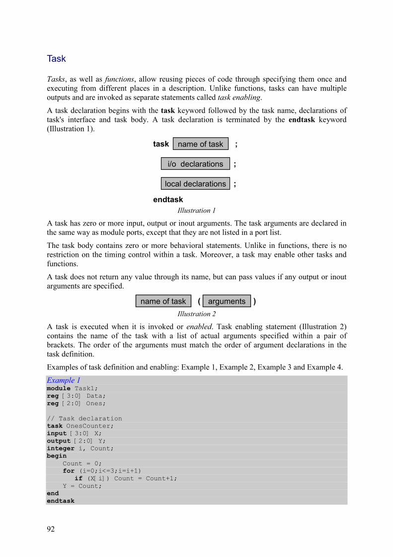
92

Task

Tasks, as well as functions, allow reusing pieces of code through specifying them once and executing from different places in a description. Unlike functions, tasks can have multiple outputs and are invoked as separate statements called task enabling.

A task declaration begins with the task keyword followed by the task name, declarations of task's interface and task body. A task declaration is terminated by the endtask keyword (Illustration 1).

endtask

task name of task

i/o declarations ;

;

local declarations ;

Illustration 1

A task has zero or more input, output or inout arguments. The task arguments are declared in the same way as module ports, except that they are not listed in a port list.

The task body contains zero or more behavioral statements. Unlike in functions, there is no restriction on the timing control within a task. Moreover, a task may enable other tasks and functions.

A task does not return any value through its name, but can pass values if any output or inout arguments are specified.

argumentsname of task ( )

Illustration 2

A task is executed when it is invoked or enabled. Task enabling statement (Illustration 2) contains the name of the task with a list of actual arguments specified within a pair of brackets. The order of the arguments must match the order of argument declarations in the task definition.

Examples of task definition and enabling: Example 1, Example 2, Example 3 and Example 4.

Example 1 module Task1; reg [3:0] Data; reg [2:0] Ones; // Task declaration task OnesCounter; input [3:0] X; output [2:0] Y; integer i, Count; begin Count = 0; for (i=0;i<=3;i=i+1) if (X[i]) Count = Count+1; Y = Count; end endtask

93

always @ (Data) // Task invocation OnesCounter (Data, Ones); endmodule

Example 2 module Task2; reg [3:0] Data; reg Check; // Task declaration task ParityCheck; input [3:0] Data; output Check; begin

Check = ^Data; end endtask

always @ (Data) // Task invocation ParityCheck (Data, Check); endmodule

Example 3 module SimpleGates1; reg A, B, AorB; reg AandB, AxorB, AxnorB; task Gates; input InA, InB; output Y1, Y2, Y3, Y4; begin Y1 = InA |InB; Y2 = InA & InB; Y3 = InA ^ InB; Y4 = ~(InA ^ InB); end endtask

always @(A or B) begin Gates (A, B, AorB, AandB, AxorB, AxnorB); end

endmodule

Example 4 module SimpleGates2;

reg A, B, AorB, AandB, AxorB; task OrGate;

94

input A, B; output Y; begin

#6 Y = A | B; end endtask task AndGate; input A, B; output Y; begin

#5 Y = A & B; end endtask task XorGate; input A, B; output Y; begin

#7 Y = A ^ B; end endtask task Gates; input InA, InB; output Y1, Y2, Y3; begin

OrGate (Y1, InA, InB); AndGate (Y2, InA, InB); XorGate (Y3, InA, InB); end endtask

always @(A or B) begin Gates (A, B, AorB, AandB, AxorB); end

endmodule

95

Time Data Type

Time is a register data type. Its purpose is to store (and make available) actual simulation time.

An object of a time type is specified with the time keyword (Example 1, Illustration 1):

;,

time register name ,

. . .

time

time register name

Illustration 1

Example 1 time Tp, Th, Ts; // Declaration of three time variables time Change_point [1:100]; // An array of times

In order to assign actual simulation time to an object of the time type the system function $time can be applied (Example 2).

Example 2 initial

act_sim_time = $time; end

The value stored in an object of the time data type is an unsigned integer. Its size is implementation-dependent, but not smaller than 64 bits.

There is no predefined relationship between simulation time stored in a time object and the real time parameters of a specified digital circuit.

96

User Defined Primitive (UDP)

User Defined Primitives (UDPs) provide a way of extending predefined gate primitives with more complex structures that can be used in the same way as language primitives.

primitive

endprimitive

port declarations

UDP body

name of UDP ( );port , , . . .port

Illustration 1

Each UDP declaration starts with the primitive keyword followed by the UDP name and port list (Illustration 1). Then each port has to be declared. The number of inputs can be one or more (maximum number depends on a compiler), but each UDP may have only one output, which has to be the first port in the port list. No bidirectional ports are allowed, as well as high impedance values. UDP body, which follows port declarations, is terminated by the endprimitive keyword.

There are two main types of UDPs: combinatorial and sequential. The UDP body is declared in different way for either of the two types.

In a combinatorial UDPs the output is determined as a function of inputs. For that reason such a primitive can be specified as a truth table. Such a table forms the UDP body and is specified between table and endtable keywords (Illustration 2). Each row contains a combination of input values and expected value of the output, separated by a colon. Each row is terminated by a semicolon. The order of inputs in each row follows the order of their declaration as ports in the port declaration section (Example 1).

table entries

input . . . outputinput

table

endtable

:

Illustration 2

Example 1 // Combinational UDPs primitive Mux2to1 (Y, Sel, A, B); output Y; input Sel, A, B; // no initialization for // combinational primitives

97

table // Sel A B : Y 0 0 ? : 0; 0 1 ? : 1; 1 ? 0 : 0; 1 ? 1 : 1; x ? ? : x; endtable endprimitive

In sequential circuits the value of the output (state) depends not only on the inputs, but also on the actual state of the circuit. This fact is reflected by the structure of the UDP body, where the table contains three groups of values (inputs, current state and next state) separated by colons (Illustration 3). Moreover, in this case it is allowed to introduce primitive initialization through the initial statement.

input . . . actual stateinput : next state:

Illustration 3

Level-sensitive sequential UDPs react to the values of inputs and the truth table is constructed with stable values (Example 2).

Example 2 // Level-sensitive sequential UDPs primitive RSLatch (Q, R, S, En); output Q; reg Q; input R, S, En;

// Initialization for // sequential primitives initial

Q = 1’b1;

table

// R S En | Q | Q* // ------------------ 0 0 1 : ? : -; 1 0 1 : ? : 0; 0 1 1 : ? : 1; 1 1 1 : ? : 1; ? ? 0 : ? : -; endtable

endprimitive

In edge-sensitive UDPs their behavior depends on the changes of the clock signal and depending on the edge the reactions of the system can be different. Because of that the truth table for the clock signal column contains specification of edges, not values (Example 3).

Example 3 // Edge-sensitive sequential UDPs primitive TFF (Q, Clk, Clr); output Q; reg Q; input Clr, Clk; // Initialization for // sequential primitives initial

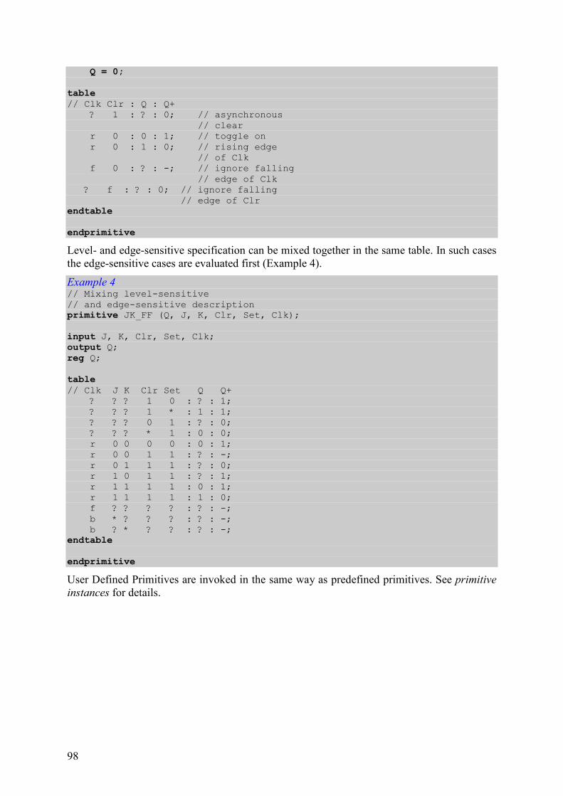
98

Q = 0;

table // Clk Clr : Q : Q+ ? 1 : ? : 0; // asynchronous // clear r 0 : 0 : 1; // toggle on r 0 : 1 : 0; // rising edge // of Clk f 0 : ? : -; // ignore falling // edge of Clk ? f : ? : 0; // ignore falling // edge of Clr endtable

endprimitive

Level- and edge-sensitive specification can be mixed together in the same table. In such cases the edge-sensitive cases are evaluated first (Example 4).

Example 4 // Mixing level-sensitive // and edge-sensitive description primitive JK_FF (Q, J, K, Clr, Set, Clk); input J, K, Clr, Set, Clk; output Q; reg Q; table // Clk J K Clr Set Q Q+ ? ? ? 1 0 : ? : 1; ? ? ? 1 * : 1 : 1; ? ? ? 0 1 : ? : 0; ? ? ? * 1 : 0 : 0; r 0 0 0 0 : 0 : 1; r 0 0 1 1 : ? : -; r 0 1 1 1 : ? : 0; r 1 0 1 1 : ? : 1; r 1 1 1 1 : 0 : 1; r 1 1 1 1 : 1 : 0; f ? ? ? ? : ? : -; b * ? ? ? : ? : -; b ? * ? ? : ? : -; endtable endprimitive

User Defined Primitives are invoked in the same way as predefined primitives. See primitive instances for details.

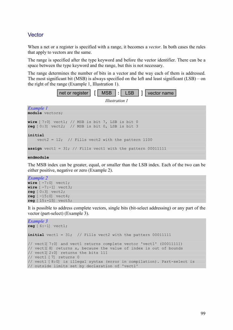
99

Vector

When a net or a register is specified with a range, it becomes a vector. In both cases the rules that apply to vectors are the same.

The range is specified after the type keyword and before the vector identifier. There can be a space between the type keyword and the range, but this is not necessary.

The range determines the number of bits in a vector and the way each of them is addressed. The most significant bit (MSB) is always specified on the left and least significant (LSB) – on the right of the range (Example 1, Illustration 1).

][ MSBnet or register : LSB vector name

Illustration 1

Example 1 module vectors; wire [7:0] vect1; // MSB is bit 7, LSB is bit 0 reg [0:3] vect2; // MSB is bit 0, LSB is bit 3 initial vect2 = 12; // Fills vect2 with the pattern 1100 assign vect1 = 31; // Fills vect1 with the pattern 00011111 endmodule

The MSB index can be greater, equal, or smaller than the LSB index. Each of the two can be either positive, negative or zero (Example 2).

Example 2 wire [-7:0] vect1; wire [-7:-1] vect3; reg [0:3] vect2; reg [-15:0] vect4; reg [15:-15] vect5;

It is possible to address complete vectors, single bits (bit-select addressing) or any part of the vector (part-select) (Example 3).

Example 3 reg [6:-1] vect1; initial vect1 = 31; // Fills vect2 with the pattern 00011111 // vect1[7:0] and vect1 returns complete vector 'vect1' (00011111) // vect1[8] returns x, because the value of index is out of bounds // vect1[2:0] returns the bits 111 // vect1 [7] returns 0 // vect1 [8:0] is illegal syntax (error in compilation). Part-select is // outside limits set by declaration of 'vect1'

100

Wait Statement

Wait statements allow level-sensitive control over the execution of a behavioral block. It blocks the execution of a block until the condition specified within brackets following the wait keyword (Illustration 1) is true. Only then the statements associated with the wait statement are executed (Example 1).

wait condition expression

statement

( )

;

Illustration 1

Example 1 // Level-sensitive latch module D_Latch (D, Clock, Q); input D, Clock; output Q; reg Q; always wait (Clock) Q = D; endmodule

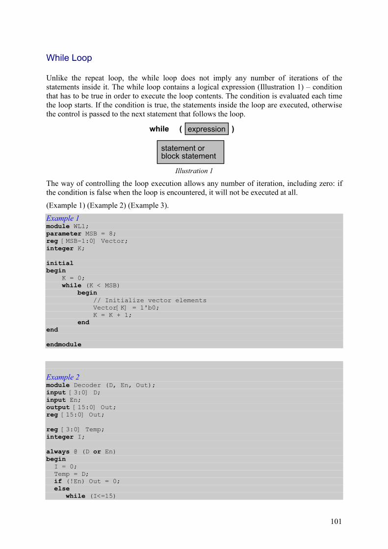
101

While Loop

Unlike the repeat loop, the while loop does not imply any number of iterations of the statements inside it. The while loop contains a logical expression (Illustration 1) – condition that has to be true in order to execute the loop contents. The condition is evaluated each time the loop starts. If the condition is true, the statements inside the loop are executed, otherwise the control is passed to the next statement that follows the loop.

statement orblock statement

while expression( )

Illustration 1

The way of controlling the loop execution allows any number of iteration, including zero: if the condition is false when the loop is encountered, it will not be executed at all.

(Example 1) (Example 2) (Example 3).

Example 1 module WL1; parameter MSB = 8; reg [MSB-1:0] Vector; integer K; initial begin

K = 0; while (K < MSB) begin // Initialize vector elements Vector[K] = 1'b0; K = K + 1; end end endmodule

Example 2 module Decoder (D, En, Out); input [3:0] D; input En; output [15:0] Out; reg [15:0] Out; reg [3:0] Temp; integer I;

always @ (D or En) begin

I = 0; Temp = D; if (!En) Out = 0; else while (I<=15)

102

begin if (Temp == I) Out[I] = 1; else Out[I] = 0; I = I+1; end end

endmodule

Example 3 module Clock3 (Clk); parameter Half_cycle = 20; // Time period = 40 output Clk; reg Clk; initial begin Clk = 1'b0; while (Clk || ~Clk) #Half_cycle Clk = ~Clk; end endmodule