constructive methods of wiener-hopf factorization || left versus right canonical wiener-hopf...
TRANSCRIPT
Operator Theory: Advances and Applications, Vol. 21 ©1986 Birkhauser Verlag Basel
LEFT VERSUS RIGHT CANONICAL WIENER-HOPF
FACTORIZATION
Joseph A. BallI) and Andr~ C. M Ran 2)
9
In this paper the existence of a right canonical Wiener-Hopf factorization for a rational matrix function is characterized in terms of a left canonical Wiener-Hopf factorization. Formulas for the factors in a right factorization are given in terms of the formulas for the factors in a given left factorization. Both symmetric and nonsymmetric factorizations are discussed.
1. INTRODUCTION
It is well known that Wiener-Hopf factorization of matrix and
opera.tor valued fUllctions has wide applications in analysis and electrical
engmeermg. Applications include convolution integral equations (see ego
[GFD, singular integral equations (see ego [CGD, Toeplitz operators, the
study of Riccati equations (see ego [W] and [H]) and, more recently, the
model reduction for linear systems. The latter application, presented in
detail by the authors in [BR 1,2] both for continuous time and discrete
time systems, lies at the basis of the present paper. We mention that
Glover [GI] first solved the model reduction problem for continuous time
systems without using Wiener-Hopf factorization.
The model reduction problem for discrete time systems as
presented m [BR 2] leads to the following question concernmg
Wiener-Hopf factorization. We are given a pxq rational matrix function
K()')=C()'I-A)-1 B with all its poles m the open unit disk, and a
number 0" > O. Cons truct the function
1) The first author was partially supported by a grant from the National Science Foundation.
2) The second author was supported by a grant from the Niels Stensen Stichting at Amsterdam.
10 Ball and Ran
(1.1 )
One needs a factorization of W(>.) of the form
(1.2) W(~) ~ X+(~-l)' [!p -Ux+(~) where X+ and its inverse is analytic on the disk. Note that (1.1) and
(1.2) constitute symmetric left and right Wiener-Hopf factorization of
W(>'), respectively. This problem was solved in [BR 21 using the
geometric factorization approach given in [BGK 11. In this paper we shall discuss the following more general
problem. Given a left canonical Wiener-Hopf factorization
with respect to a contour r, where Y + and Y _ are gIven m realization
form, give necessary and sufficient conditions for the existence of a right
canonical Wiener-Hopf factorization
and provide formulas for X and X+ m realization form. This IS discussed
m Section 2.
In Section 3 we give applications of the mam result of Section 2
to the invertibility of singular integral operators. As is well known the
invertibility of the singular integral operator on LP(r), where r is a
contour in the complex plane {:, with symbol W is equivalent to the
existence of a right canonical Wiener-Hopf factorization for W on r. Theorem 2.1 then gives necessary and sufficient conditions for the
invertibility of the singular integral operator with symbol W under the
assumption that the singular integral operator with symbol W- 1 (or with
Canonical factorization 11
symbol WT ) IS invertible and the right canonical factorization of W- 1
(respectively WT ) IS known. We thank Kevin Clancey for pointing out to
us this application of our main result.
In Sections 4 and 5 we indicate how symmetrized verSiOns of the
factorization problem can be handled also as a direct application of
Theorem 2.1. Section 4 deals with the situation where the symmetry is
with respect to the unit circle; this is the case which comes up for
discrete time systems. In Section 5 the symmetry is with respect to the
lffiagmary axis; this is germane to model reduction for con tinuous time
systems. In this way we may view some factorization formulas from [BR
1,2] needed for the model reduction problem as essentially specializations
of the more general formulas in Theorem 2.1.
2. LEFT AND RIGHT CANONICAL WIENER-HOPF
FACTORIZATION
In this section we shall analyze the existence of a right
canonical Wiener-Hopf factorization for a given rational matrix function in
terms of a gIven left canonical Wiener-Hopf factorization. The
factorizations are with respect to some fixed but general contour r m
the complex plane. The analysis is built on the geometric approach to
factorization gIven m [BGK I].
terminology from [BGK I].
We first establish some notation and
By a Cauchy contour r we mean the positively oriented
boundary of a bounded Cauchy domain in the complex plane <C; such a
contour consists of finitely many nonintersecting closed rectifiable Jordan
curves. We denote by F + the interior domains of r and by F the
complement of its closure F + in the extended complex plane <CU{oo}.
Now suppose that W is a rational mxm matrix function invertible
12 ball and Ran
at 00 and with no poles or zeros on the contour r. By a right
canonical (spectral) factorization of W with respect to r we mean a
factorization
(2.1) ()..Er)
where Wand W + are also rational mxm matrix functions such that W
has no poles or zeros on F _ (including 00) and W + has no poles or zeros
on F +. If the factors W _ and W + are interchanged in (2.1), we speak of
a left canonical (spectral) factorization.
We assume throughout that all matrix functions are analytic and
invertible at 00; without loss of generality we may then assume that the
value at 00 is the identity matrix I. By a realization for the matrix m
function W we mean a representation for W of the form
Here A is an nxn matrix (for some n) while C and Bare mxn and nxm
matrices respectively.
Left and right canonical factorizations are discussed at length in
the book [BGK 1]. There it is shown how to compute realizations for the
factors W _, W + for a right canonical factorization W=W _ W + if one knows
a realization W()")=Im +C()"In _A)-I B for W. We shall suppose that we
know the factors Y + and Y of a left canonical factorizations
W()..)=Y ()")Y ()..), say + -
and
Canonical factorization 13
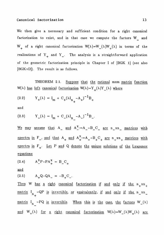
We then give a necessary and sufficient condition for a right canonical
factorization to exist, and in that case we compute the factors Wand
W + of a right canonical factorization W(A)=W jA)W +(A) in terms of the
realizations of Y + and Y _. The analysis is a straightforward application
of the geometric factorization principle in Chapter I of [BGK 1] (see also
[BGKvDj). The result is as follows.
THEOREM 2.1. Suppose that the rational mxm matrix function
W(>") has left canonical factorization W(>")=Y +(>")Y _(>..) where
and
and AX:=A -B C are n xn matrices with - - - -- - -
spectra m F , and that A and A x:=A -B Care n xn matrices with ---- +- + + ++- + +=..:..:...:.::.=
spectra m F +. Let P and Q denote the unique solutions of the Lyapunov
equations
(2.4) AXp_PA x - +
(2.5) A Q-QA = -B C . + - + -
Then W has ~ right canonical factorization if and only if the n + xn +
matrix I -QP IS invertible, .2!" equivalently, .if and only if the n _ xn n+
matrix In -PQ IS invertible. When this ~ the case, the factors W (>..)
and W +(>..) for ~ right canonical factorization W(>")=W _(>..)W +(>..) are
14 Ball and Ran
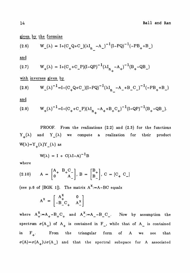
given ~ the formuias
(2.6) W_(>') = I+(C+Q+CJ(>'In -AJ-1(I-PQ)-1(-PB+ +BJ
and
with inverses given ~
and
PROOF. From the realizations (2.2) and (2.3) for the functions
Y +(>.) and Y _(>.) we compute a realization for their product
W(>')=Y +(>')Y _(>.) as
W(>.) = I + C(>'I-A)-l B
where
(see p.6 of [BGK 11). The matrix AX:=A-BC equals
where A~:=A+ -B+C+ and AX:=A -B C. Now by assumption the
spectrum u(A+) of A+ IS contained in F _, while that of A is contained
In F+. From the triangular form of A we see that
u(A)=u(A+)Uu(A_) and that the spectral subspace for A associated
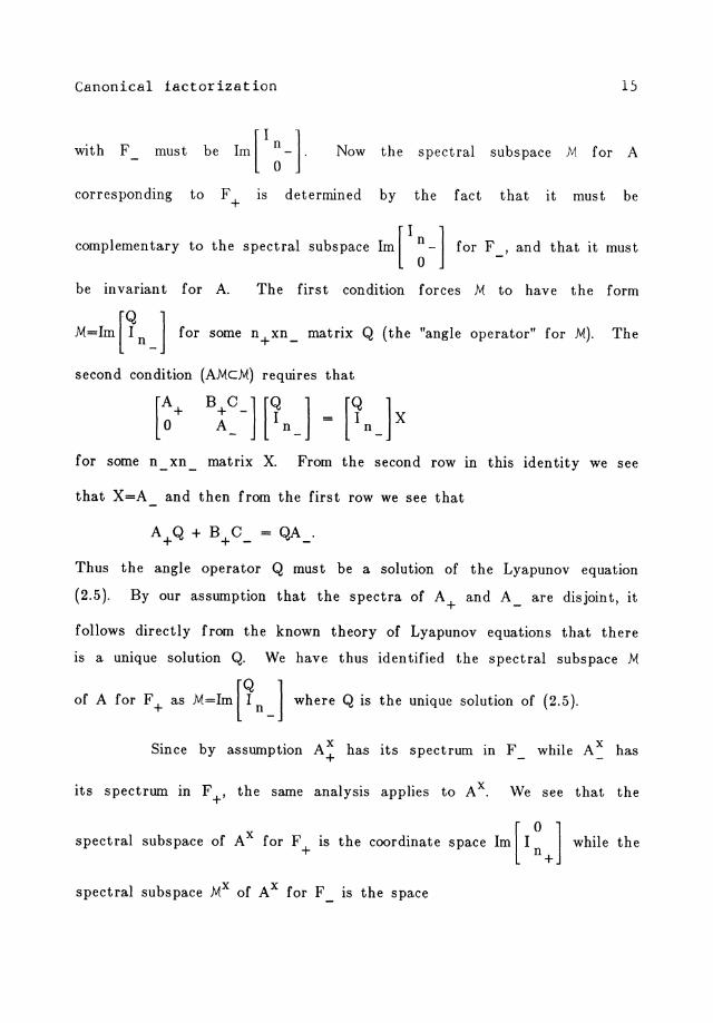
Canonical iactorization 15
with F Now the spectral subspace M for A
corresponding to F+ IS determined by the fact that it must be
complementary to the spectral subspace Im[I~-l for F , and that it must -
be invariant for A. The first condition forces M to have the form
M=lm [~n _] for some n+xn_ matrix Q (the "angle operator" for M). The
second condition (AMCM) requires that
for some n xn matrix X. From the second row ill this identity we see
that X=A and then from the first row we see that
A+Q + B+C_ = QA_.
Thus the angle operator Q must be a solution of the Lyapunov equation
(2.5). By our assumption that the spectra of A+ and A_ are disjoint, it
follows directly from the known theory of Lyapunov equations that there
is a unique solution Q. We have thus identified the spectral subspace M
of A for F + as M=Im [~n _] where Q is the unique solution of (2.5).
Since by assumption A: has its spectrum in F while A x has
its spectrum ill F +' the same analysis applies to AX. We see that the
spectral subspace of AX for F + IS the coordinate space 1m [ I: + 1 while the
spectral subspace MX of AX for F IS the space
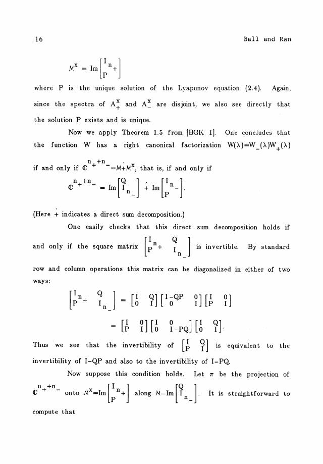
16 Ball and Ran
where P is the unique solution of the Lyapunov equation (2.4). Again,
since the spectra of A~ and A: are disjoint, we also see directly that
the solution P exists and is unique.
Now we apply Theorem 1.5 from [BGK 11. One concludes that
the function W has a right canonical factorization W(A)=W _(A)W +(A)
n +n . if and only if C + - =M+Mx, that is, if and only if
n++n C -
(Here + indicates a direct sum decomposition.)
One easily checks that this direct sum decomposition holds if
[ I QI n ]I·S I·nvertl·ble. By standard and only if the square matrix P n +
row and column operations this matrix can be diagonalized III either of two
ways:
[~n+ Q ] _ [I ~] [I OQP n [~ n In - 0
[~ n [6 ~ -PQ] [6 ~].
Thus we see that the invertibility of [~ ~] IS equivalent to the
invertibility of I-QP and also to the invertibility of I-PQ.
Now suppose this condition holds. Let IT be the projection of
Cn++n _ onto MX=lm[~n+] along M=lm[~n_]. It is straightforward to
compute that
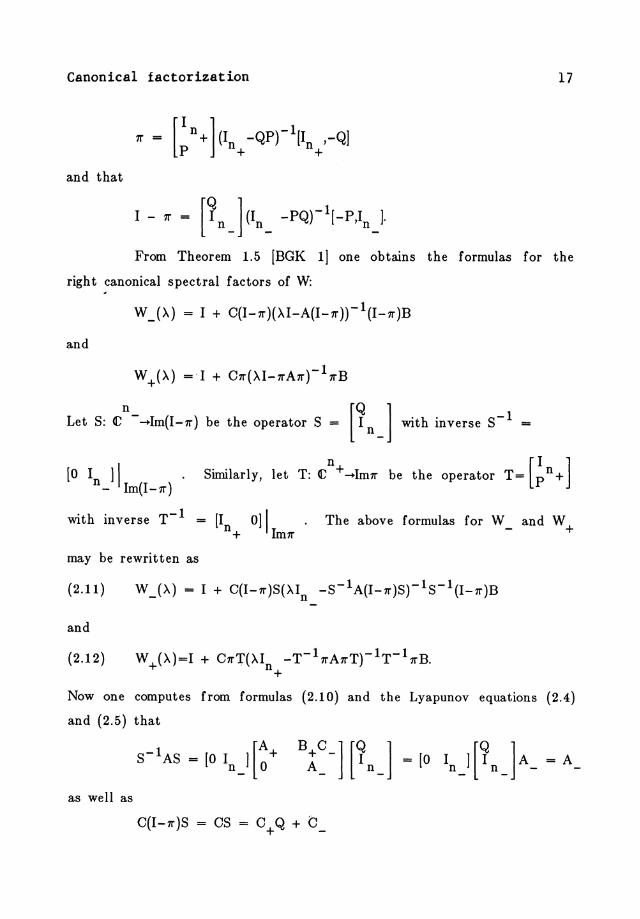
Canonical factorization 17
and that
From Theorem 1.5 [BGK 11 one obtains the formulas for the
right canonical spectral factors of W:
W _(),) = I + C(1-rr)(),I-A(I-rr))-1(I-rr)B
and
Let S: {; n_ -+lm(l-rr) be the operator S = [~n J with inverse S-1 =
[0 I II . Similarly, let T:{;n+-+lmrr be the operator T=[~n+] n _ Im(l-rr)
. h . T-1 WIt Inverse [I 011 . The above formulas for Wand W n+ Imrr - +
may be rewritten as
(2.11 )
and
W +(),)=I + CrrT(),ln -T-1rrArrT)-I T-l rrB. +
(2.12)
Now one computes from formulas (2.10) and the Lyapunov equations (2.4)
and (2.5) that
S-IAS = [0 In_I[~+ B~~_] [~nJ = [0 In_I[~nJA- = A
as well as
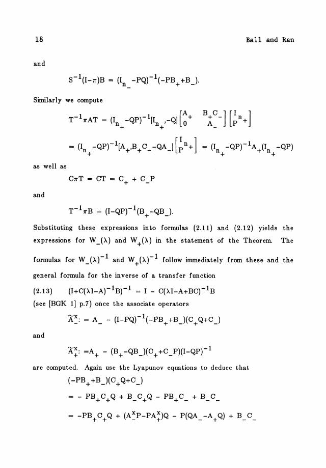
18 Ball and Ran
and
S-I(I-lI")B = (I _PQ)-I(_PB +B ). n + -
Similarly we compute
as well as
and
Substituting these expressions into formulas (2.11) and (2.12) yields the
expressions for W _(>.) and W +(>.) in the statement of the Theorem. The
formulas for W _(>.)-1 and W +(>.)-1 follow immediately from these and the
general formula for the inverse of a transfer function
(2.13)
(see [BGK 11 p.7) once the associate operators
A~: = A_ - (I_PQ)-I(_PB+ +Bj(C+Q+C_)
and
are computed. Again use the Lyapunov equations to deduce that
(-PB+ +Bj(C+Q+Cj
- PB+C+Q + B_C+Q - PB+C_ + B C
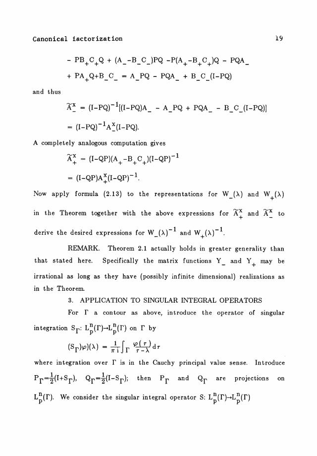
Canonical factorization
and thus
- PB+C+Q + (A_ -B_CJPQ -P(A+ -B+C+)Q - PQA_
+ PA+Q+B_C_ = A_PQ - PQA_ + B_CjI-PQ)
x: = (I-PQ)-1[(I-PQ)A_ - A_PQ + PQA_ - B_CjI-PQ)]
= (I-PQ)-1A:(I-PQ).
A completely analogous computation gives
x: = (I-QP)(A+-B+C+)(I-QP)-1
= (I-QP)A~(I-QP)-1.
19
Now apply formula (2.13) to the representations for W j>-) and W +(>-)
in the Theorem together with the above expressions for X~ and Xx to
derive the desired expressions for W _(>-)-1 and W +(>-)-1.
REMARK. Theorem 2.1 actually holds in greater generality than
that stated here. Specifically the matrix functions Y _ and Y + may be
irrational as long as they have (possibly infinite dimensional) realizations as
in the Theorem.
3. APPLICATION TO SINGULAR INTEGRAL OPERATORS
For r a contour as above, introduce the operator of singular
integration Sr: L~(r)""'L~(r) on r by
(Sr)<p)(>-) = rr\ I r <p)!>-) dT
where integration over r is in the Cauchy principal value sense. Introduce
Pr=t(I+S r ), Qr=t(I-S r ); then P r and Qr are projections on
L~(r). We consider the singular integral operator S: L~(r)""'L~(r)
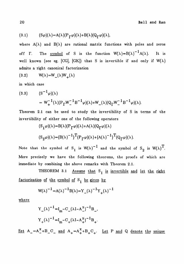
20 Ball and Ran
(3.1) (8cp)( >. )=A( >.)(P rcp)(>, )+B(>' )(QrCP)( >.),
where A(>') and B(>') are rational matrix functions with poles and zeros
off r. The symbol of 8 is the function W(>')=B(>.)-1 A(>'). It is
well known (see ego [OGI, [GKJ) that 8 is invertible if and only if W(>.)
admits a "right canonical factorization
(3.2) W(>')=W _(>.)W +(>.)
in which case
(3.3) (8- 1cp)(>.)
= W~ 1 (>.)(PrW= I B-lcp)(>.)+W _(>.)(QrW= I B-1cp)(>.).
Theorem 2.1 can be used to study the invertibility of 8 in terms of the
invertibility of either one of the following operators
(81 cp)(>.)=B(>.)(Prcp)(>.)+A(>.)(QrCP)(>')
(82cp)(>. )={B(>') -I} T (P rcp)( >. )+{A(>') -I} T (QrCP)(>').
Note that the symbol of 81 is W(>.)-1 and the symbol of 82 is W(>.)T.
More precisely we have the following theorems, the proofs of which are
immediate by combining the above remarks with Theorem 2.1.
THEOREM 3.1 Assume that 81 is invertible and let the right
factorization of the symbol of 81 be given II
y _(>.)-1=lm -0 _(>.I_A~)-1B_,
Y (>.)-1=1 -0 (>.I_AX)-1 B + m + + +.
Let P and Q denote the unique
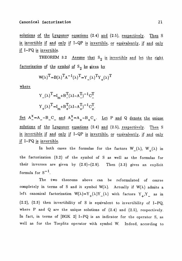
Canonical factorization 21
solutions of the Lyapunov equations (2.4) and (2.5), respectively. Then S
is invertible if and only if I-QP !5! invertible, or equivalently, if and only
if I-PQ ~ invertible.
THEOREM 3.2 Assume that 8 2 ~ invertible and let the right
factorization 2! the symbol of 8 2 be given Qy
W().)T =B().)TA -l().)T =y _().)Ty +().) T
Y _().)T =Im +B~()'I-A~)-lC~
y ().)T=I +BT()'I_AT)-lCT. + m + + +
8et A x =A -B _ C _ and A! =A + -B + C +' Let P and Q denote the unique
solutions of the Lyapunov equations (2.4) and (2.5), respectively. Then 8
is invertible if and only if I-QP ~ invertible, .2!' equivalently, if and only
if I-PQ is invertible.
In both cases the formulas for the factors W_().), W+().) in
the factorization (3.2) of the symbol of 8 as well as the formulas for
their inverses are given by (2.6)-(2.9).
formula for 8- 1.
Then (3.3) gives an explicit
The two theorems above can be reformulated of course
completely in terms of 8 and it symbol W().). Actually if W()') admits a
left canonical factorization W()')=Y +()')Y _().) with factors Y +,Y _ as m
(2.2), (2.3) then invertibility of 8 is equivalent to invertibility of I-PQ,
where P and Q are the unique solutions of (2.4) and (2.5), respectively.
In fact, in terms of [BGK 2] I-PQ is an indicator for the operator 8, as
well as for the Toeplitz operator with symbol W. Indeed, according to
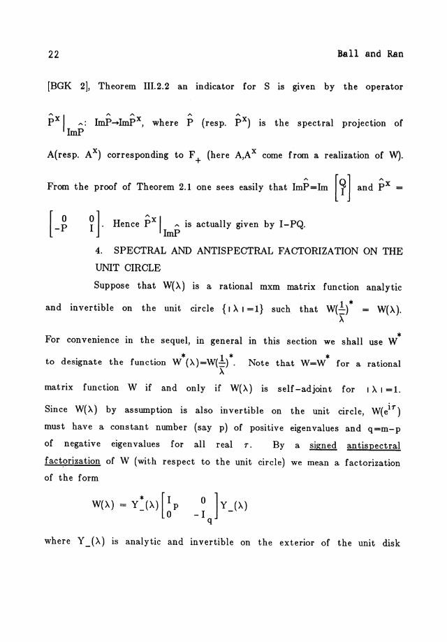
22 Ball and Ran
[BGK 2], Theorem III.2.2 an indicator for S IS given by the operator
pX I A: ImP-+ImPX, where P (resp. pX) IS the spectral projection of ImP
A(resp. AX) corresponding to F + (here A,Ax come from a realization of W).
From the proof of Theorem 2.1 one sees easily that ImP=Im [~l and pX
Hence pX I A is actually given by I-PQ. ImP
4. SPECTRAL AND ANTISPECTRAL FACTORIZATION ON THE
UNIT CIRCLE
Suppose that W( A) IS a rational mxm matrix function analytic
and invertible on the unit circle {I A I =1} such that W(.!/ = W(A). A
* For convemence 10 the sequel, in general 10 this section we shall use W
* 1 * * to designate the function W (A)=W(=). Note that W=W for a rational A
matrix function W if and only if W( A) is self -adjoin t for I A I = 1.
Since W(A) by assumption is also invertible on the unit circle, W(eiT )
must have a constant number (say p) of positive eigenvalues and q=m-p
of negative eigenvalues for all real T. By a signed antispectral
factorization of W (with respect to the unit circle) we mean a factorization
of the form
where Y _(A) is analytic and invertible on the exterior of the unit disk
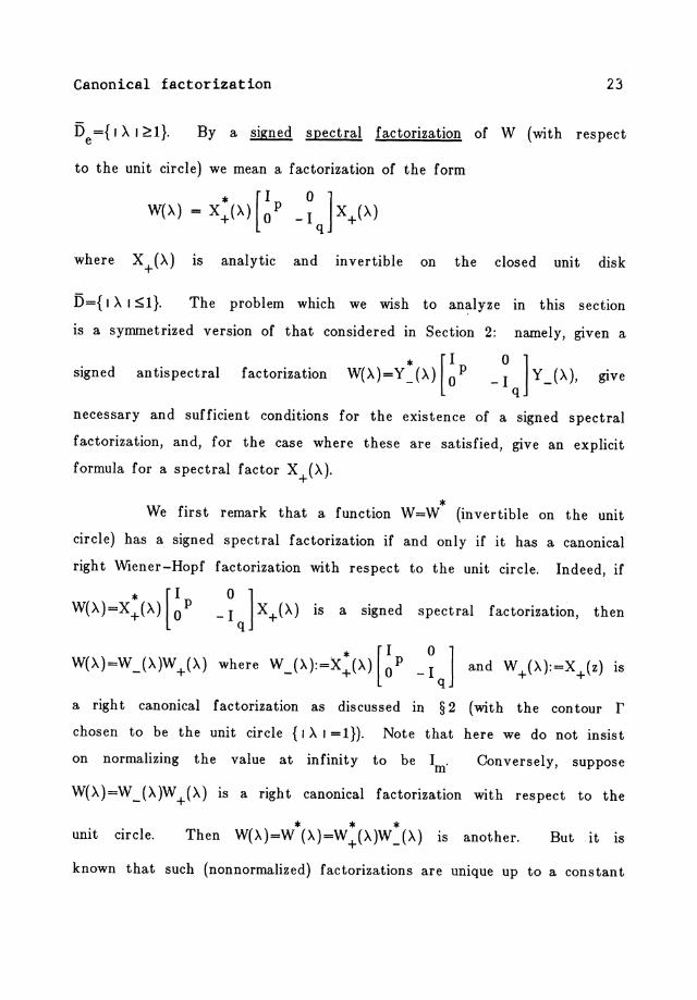
Canonical factorization 23
i5 ={ I A I ~1}. e By a signed spectral factorization of W (with respect
to the unit circle) we mean a factorization of the form
where X+(A) IS analytic and invertible on the closed unit disk
D={IAI~l}. The problem which we wish to analyze In this section
is a symmetrized version of that considered in Section 2: namely, given a
signed antispectral factorization W(A)=Y:(A) [~p _ ~ J Y _(A), gIve
necessary and sufficient conditions for the existence of a signed spectral
factorization, and, for the case where these are satisfied, give an explicit
formula for a spectral factor X +(A).
* We first remark that a function W=W (invertible on the unit
circle) has a signed spectral factorization if and only if it has a canonical
right Wiener-Hopf factorization with respect to the unit circle. Indeed, if
-~qlX+(A) is a signed spectral factorization, then
W(A)=W _(A)W +(A) where W _(A):=X:(A) [~p _ ~ q] and W +(A):=X+(z) IS
a right canonical factorization as discussed in § 2 (with the contour r chosen to be the unit circle {I A I =1}). Note that here we do not insist
on normalizing the value at infinity to be 1m' Conversely, suppose
W(A)=W jA)W +(A) is a right canonical factorization with respect to the
* * * unit circle. Then W(A)=W (A)=W +(A)W _(A) is another. But . it is
known that such (nonnormalized) factorizations are unique up to a constant
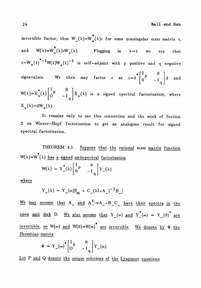
24 Ball and Ran
* invertible factor; thus W (> .. )=W (A)C for some nonsingular mxm matrix c, - +
and Plugging In A=1 we see that
c=W +(1) *-IW(1)W +(1)-1 is self -adjoint with p positive and q negative
eigenvalues. We then may factor c as c=d * [ ~ p _ ~ q 1 d and
W(A)=X:(A) [~p X+(A)=dW +(A).
_ ~ J X+(A) IS a signed spectral factorization, where
It remains only to use this connection and the work of Section
2 on Wiener-Hopf factorization to get an analogous result for signed
spectral factorization.
THEOREM 4.1. Suppose that the rational mxm matrix function
* W(A)=W (A) has .! signed antispectral factorization
Y (A) = Y (00)[1 + C (AI-A )-IB 1 - - m - - -
* * open unit disk D. We also assume that Y joo) and Y _(00) = Y _(0) ~
* invertible, ~ W(oo) and W(O)=W(oo) are invertible. We denote h \II the
Hermitian matrix
Let P and Q denote the unique solutions of the Lyapunov equations
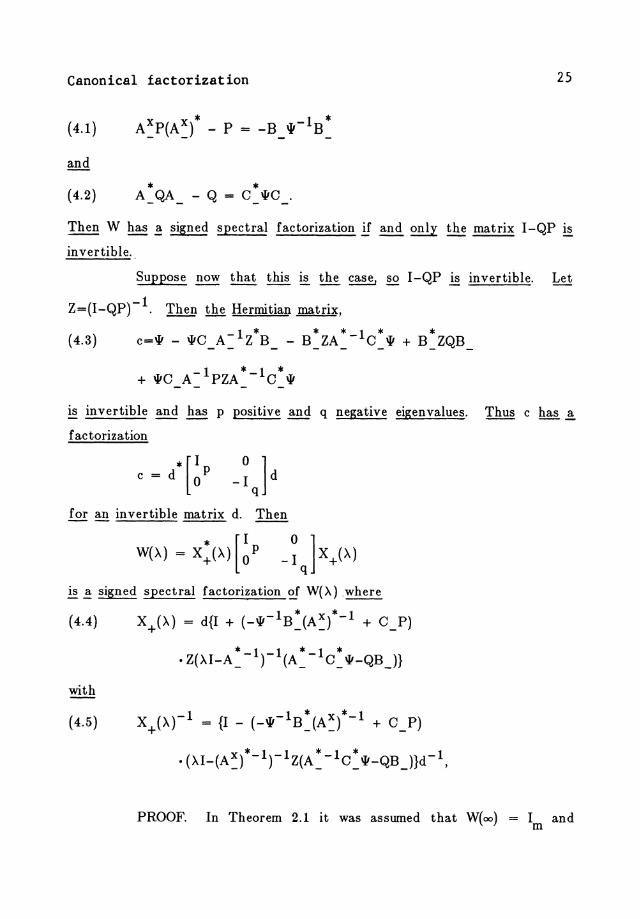
Canonical factorization 25
( 4.1)
Then W has! signed spectral factorization i! and only the matrix I-QP ~
invertible.
Suppose ~ that this is the case. §.2 I-QP is invertible. Let
Z=(I_QP)-I. Then the Hermitian matrix,
1* * *1* * (4.3) c=W - WC_A= Z B_ - B_ZA_ - C_ W + B_ZQB_
IS invertible and has p positive and q negative eigenvalues. Thus c has ~
f ac toriza tion
* [I c = d op
for ~ invertible matrix d. Then
is ~ signed spectral factorization of W(A) .where
(4.4) X+(A) = d{I + (_W- 1B:(A:)*-1 + C_P)
. Z(AI-A: -1)-I(A: -IC: W-QB_n
with
(4.5) X+(A)-1 = {I - (_w- 1B:(A:)*-1 + C_P)
• (AI-(A:) *-I)-IZ(A: -IC: w-QB J}d- 1,
PROOF. In Theorem 2.1 it was assumed that W(oo) I and m
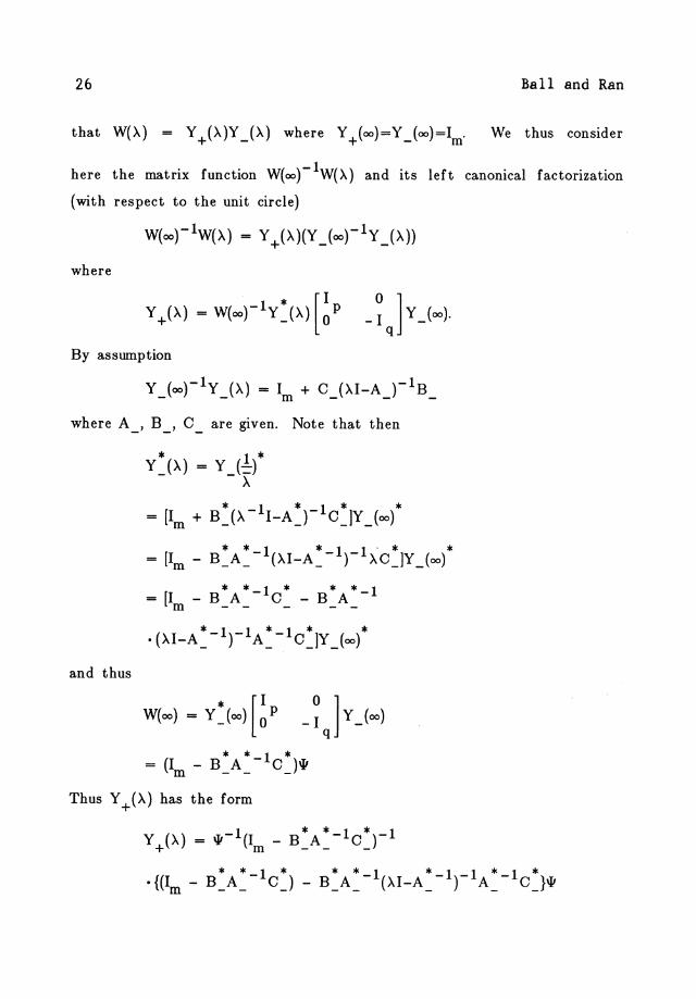
26 Ball and Ran
that W()") = Y +()")Y _()..) where Y +(oo)=Y _(oo)=lm' We thus consider
here the matrix function W(oo)-IW()..) and its left canonical factorization
(with respect to the unit circle)
where
By assumption
Y (oo)-ly ()..) = I + C ()"I-A )-I B - - m - - -
where A , B _, C _ are given. Note that then
**1* **1 = [I - B A - C - B A -m - - - --
and thus
* [I W(oo) = Y Joo) 0 P
* * 1 * = (1m - B_A_ - CJIII
Thus Y +()..) has the form
Y ()..) = 111- 1(1 _ B*A*-IC*)-1 + m - - -
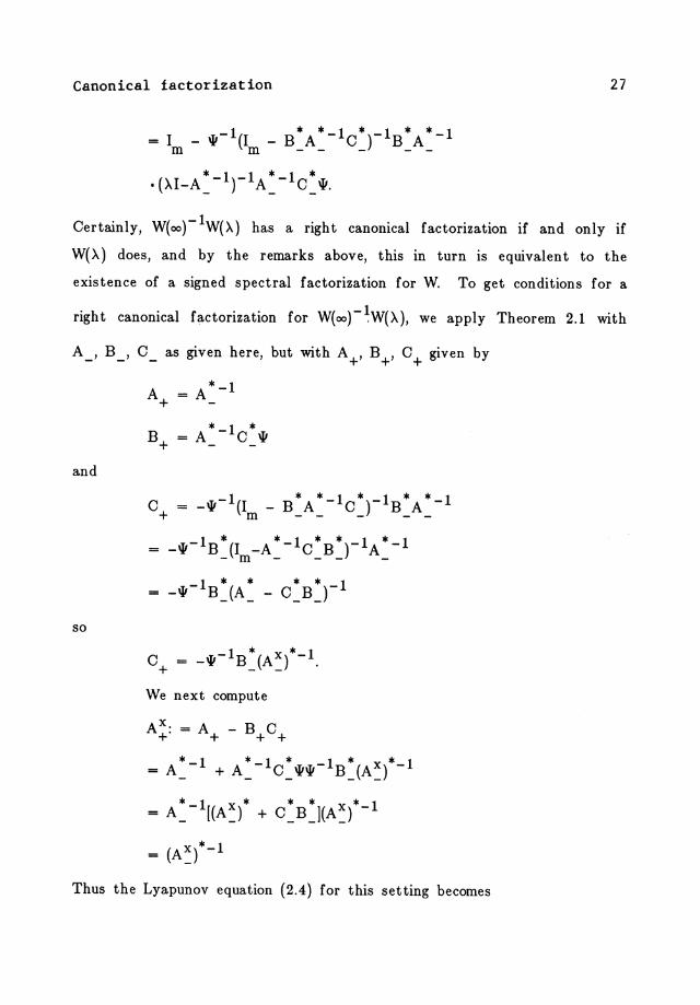
Canonical factorization 27
1 **1* 1**1 = 1 - \II - (I - B A - C ) - B A -m m -- - --
Certainly, W(oo)-lW(A) has a right canonical factorization if and only if
W(A) does, and by the remarks above, this in turn is equivalent to the
existence of a signed spectral factorization for W. To get conditions for a
right canonical factorization for W(OO)-~W(A), we apply Theorem 2.1 with
A _, B _, C _ as given here, but with A +' B +' C + given by
A+ = A*-l
and
so
We next compute
*1 * ** *1 = A_ - [(A:) + C_BJ(A:) -
= (A:)*-l
Thus the Lyapunov equation (2.4) for this setting becomes
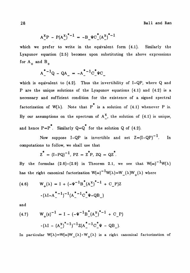
28 Ball and Ran
which we prefer to write in the equivalent form (4.1). Similarly the
Lyapunov equation (2.5) becomes upon substituting the above expressions
for A+ and B+
• 1 • 1 • A_ - Q - QA_ = -A_ - 0_1110
which is equivalent to (4.2). Thus the invertibility of I-QP, where Q and
P are the unique solutions of the Lyapunov equations (4.1) and (4.2) is a
necessary and sufficient condition for the existence of a signed spectral
• factorization of W(X). Note that P is a solution of (4.1) whenever Pis.
By our assumptions on the spectrum of A~, the solution of (4.1) is unique,
• • and hence P=P. Similarly Q=Q for the solution Q of (4.2).
Now suppose I-QP is invertible and set Z=(I_QP)-I. In
computations to follow, we shall use that
• 1 • • Z = (1-PQ) - , PZ = Z P, ZQ = QZ .
By the formulas (2.6)-(2.9) in Theorem 2.1, we see that W(oo)-IW(X)
has the right canonical factorization W(oo)-IW(X)=W _(X)W +(X) where
(4.6) W+(X) = I + (_V-lB:(A~)·-1 + O_P)Z
• (XI-A: -1)-I(A: -10 : 1I1-QB_)
and
(4.7) W+(z)-1 = I - (_1I1-1B:(A~)·-1 + O_P)
• (XI - (A~)·-I)-IZ(A: -1 0 : 111 - QB _).
In particular W(~)=W(oo)W _(~). W +(~) is a right canonical factorization of
Canonical factorization 29
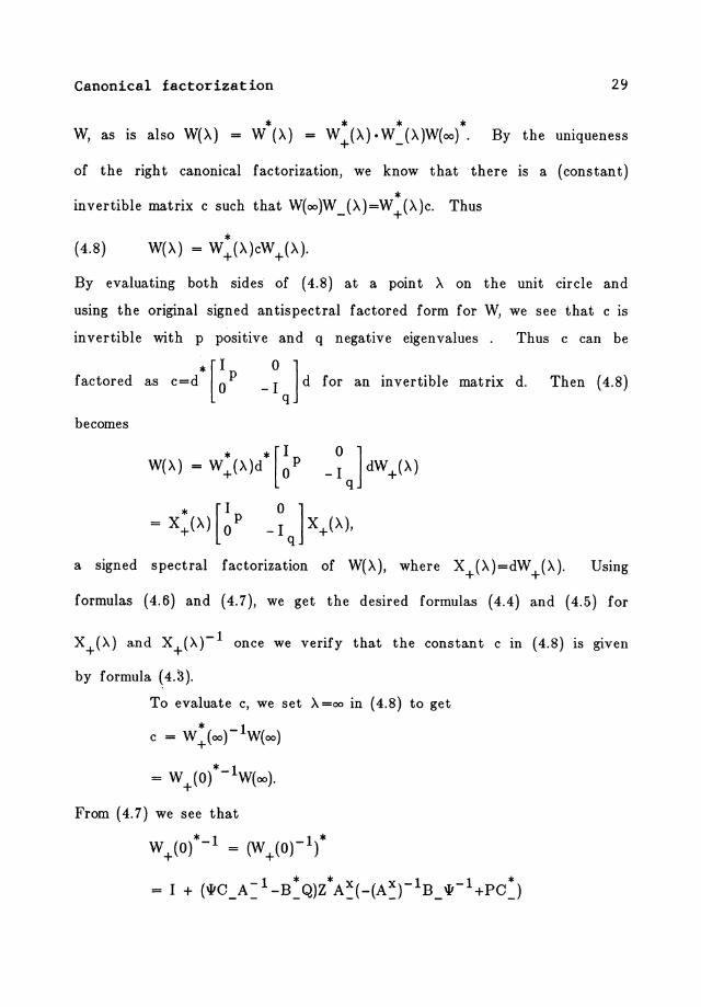
* * * * W, as is also W(>.) = W (>.) W +(>.). W J>.)W(oo). By the umqueness
of the right canonical factorization, we know that there is a (constant)
* invertible matrix c such that W(oo)W j>.)=W +(>.)c. Thus
By evaluating both sides of (4.8) at a point >. on the unit circle and
using the original signed antispectral factored form for W, we see that c IS
invertible with p positive and q negative eigenvalues. Thus c can be
factored "" e~d' [~p _ ~ J d for an invertible matrix d. Then (4.8J
becomes
* *[1 W(>.) = W +(>.)d 0 p
a signed spectral factorization of W(>'), where X+(>')=dW +(>.). Using
formulas (4.6) and (4.7), we get the desired formulas (4.4) and (4.5) for
X+(A) and X+(A)-l once we verify that the constant c in (4.8) is given
by formula (4.3).
To evaluate c, we set A =00 in (4.8) to get
* 1 c = W +(00)- W(oo)
* 1 = W +(0) - W(oo).
From (4.7) we see that
W +(0) *-1 = (W +(0)-1) *
= I + (WC_A=1_B:Q)Z*A:(-(A:)-lB_W-1+PC:)
30 ball and Ran
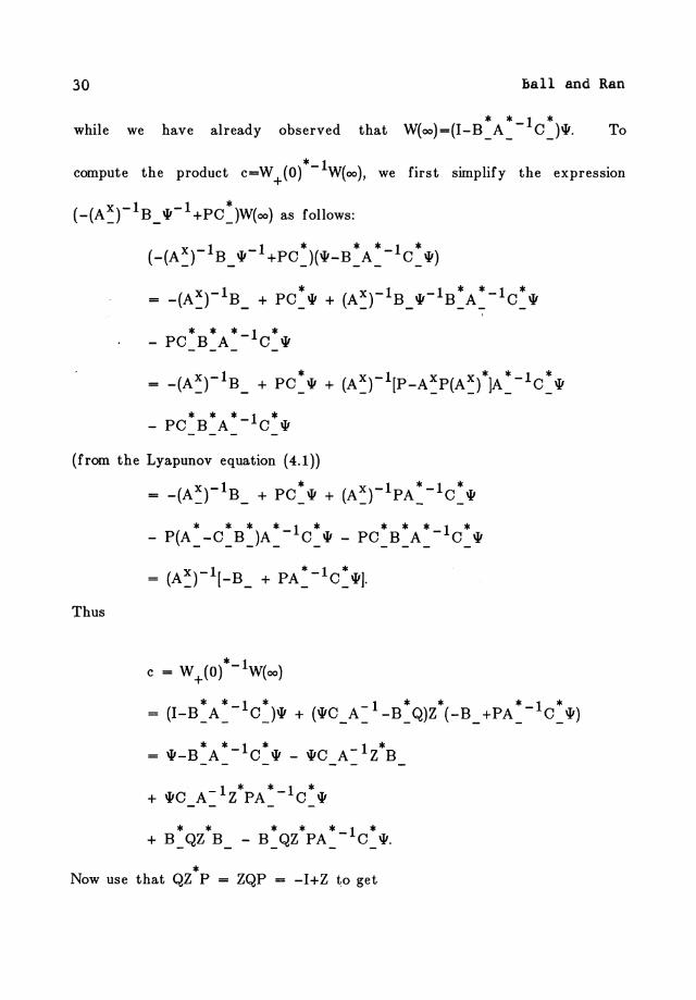
while we have already observed that * * 1 * W(oo)=(I-B _A _ - 0 Jw. To
* 1 compute the product c=W +(0) - W(oo) , we first simplify the expression
(-(A~)-IB_w-l+PO:)W(oo) as follows:
1 1 * **1* (-(A x) - B w- +PO )(w-B A - 0 w) - - - - - -
* * * 1 * - PO B A - 0 w
* * * 1 * - PO B A - 0 w
(from the Lyapunov equation (4.1))
Thus
= _(A~)-IB_ + PO: w + (A~)-lpA:-I0: w
* ** *1* ***1* - P(A _ -0 _ B JA _ - 0 _w - PO _ B _A _ - O_w
= (A~)-I[_B_ + PA: -10 : wJ.
* * 1 * 1 * = w-B A - 0 w - WO A - Z B - - -1 * * 1 * + WO A - Z P A - 0 w - -
* Now use that QZ P = ZQP = -I+Z to. get
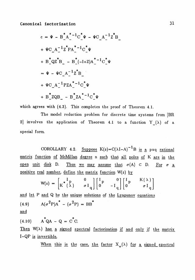
Canonical factorization 31
* *-1 * -1 * c = 111 - B A 0 111 - 1110 A Z B
1 * * 1 * + 1110 A - Z P A - 0 111 - -
+ 1110 A-1pZA*-10*1I1 - -
which agrees with (4.3). This completes the proof of Theorem 4.1.
The model reduction problem for discrete time systems from [BR
21 involves the application of Theorem 4.1 to a function Y J)..) of a
special form.
OOROLLARY 4.2. Suppose K(z)=C()..I-A)-1 B is ~ pxq rational
matrix function of McMillan degree n such that all poles of K are in the
open unit disk D. Thus ~ may assume that o-(A) c D. For 0- ~
positive real number, ~ the matrix function W(z) Q.y
and let P and Q be the unique solutions 2f the Lyapunov equations
(4.9) 2 * 2 * A(o- P)A - (0- P) = BB
* * (4.10) A QA - Q 00.
Then W()") has ~ signed spectral factorization if and only if the matrix
I-QP is invertible.
When this is the case, the factor X+()") for ~ signed spectral
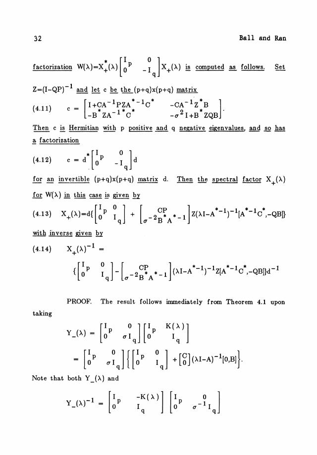
32 Ball and Ran
* [I factorization W().)=X+().) 0 P _ ~ q 1 X+().) is computed !:§.. follows. Set
Z=(I_QP)-1 and let c be the (p+q)x(p+q) matrix
(4.11)
Then c is Hermitian with p positive and q negative eigenvalues. and AQ has
a factorization
(4.12) * [I c = d. oP
for an invertible (p+q).x(p+q) matrix d. Then the spectral factor X+().)
for W()') in this case g; given £I
(4.13) X+()')=d{[~P ~ql + [oo-2~~A*-1 ]Z()'I_A*-1)-1[A*-1 C*,_QB]}
with inverse given III
(4.14) X +(). )-1
{[ ~ p ~ q] - [00 - 2~~ A * -1 ] ()'I-A *-1)-1Z[A *-1 C*,_QB]}d-1
PROOF. The result follows immediately from Theorem 4.1 upon
taking
Y_(X) - [~p u~J [~p K~:)l
- [!p u~J {[~p ~J + [~1(XI-A)-110'BI} Note that both Y _ ().) and
Canonical factorization 33
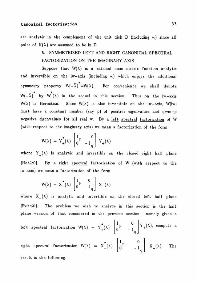
are analytic in the complement of the unit disk D (including 00) SInce all
poles of K(A) are assumed to be in D.
5. SYMMETRIZED LEFT AND RIGHT CANONICAL SPECTRAL
FACTORIZATION ON THE IMAGINARY AXIS
Suppose that W( A) is a rational mxm matrix function analytic
and invertible on the iw-axis (including 00) which enjoys the additional
- * symmetry property W( -A) =W(A). For convenience we shall denote
- * * W(-A) by W (A) in the sequel in this section. Thus on the lw-aXlS
W(A) IS Hermitian. Since W(A) is also invertible on the iw-axis, W(iw)
must have a constant number (say p) of positive eigenvalues and q=m-p
negative eigenvalues for all real w. By a left spectral factorization of W
(with respect to the imaginary axis) we mean a factorization of the form
where Y +(A) is analytic and invertible on the closed right half plane
{ReA~O}. By a right spectral factorization of W (with respect to the
iw axis) we mean a factorization of the form
where X_(A) is analytic and invertible on the closed left half plane
{ReA:50}. The problem we wish to analyze In this section is the half
plane version of that considered in the previous section: namely given a
left spectral factorization W(A)
* right spectral factorization W(A) XjA)
resul t is the following.
o ]Y+(A), -I q
compute a
The
34 Ball and Ran
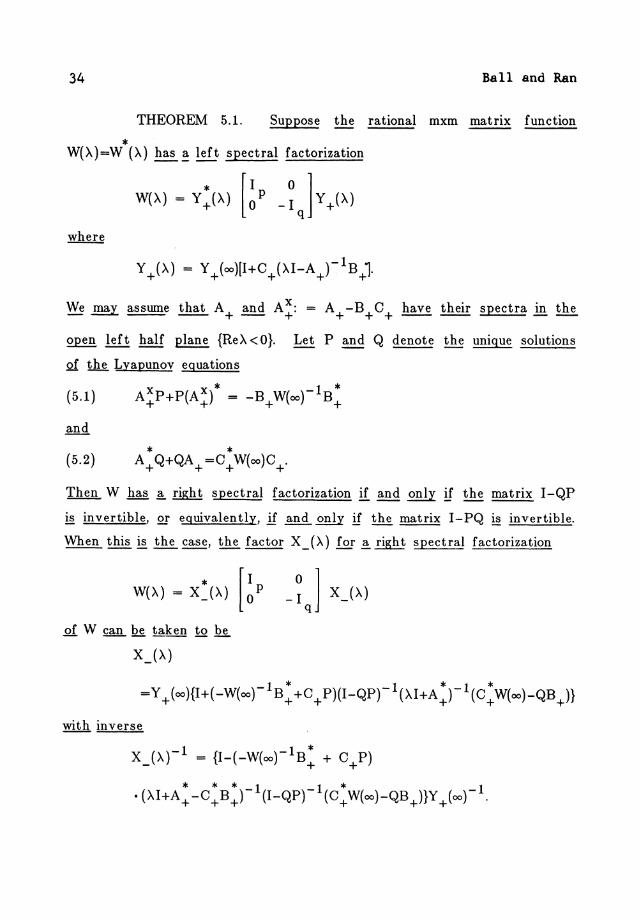
THEOREM 5.1. Suppose the rational mxm matrix function
* W(A)=W (A) has ~ left spectral factorization
We may ~e that A+ and A~: = A+ -B+O+ have their spectra in the
open left half plane {ReA < a}. Let P and Q denote the unique solutions
of the Lyapunov equations
(5.1 )
Then W has ~ right spectral factorization if and only!! the matrix I-QP
~ invertible, .Q! equivalently, if and only if the matrix I-PQ ~ invertible.
When this is the ~, the factor X_(A) for ~ right spectral factorization
X_(A)
=Y + (oo){I+ ( _W(oo)-l B: +0+ P)(I-QP)-l(AI+A :)-1(0: W(oo)-QB +)}
with inverse
x (A) -1 = {I - ( - W( 00) -1 B * + 0 P) - + +
* **1 1* 1 • (AI+A+ -O+B+)- (I-QP)- (O+W(oo)-QB+)}Y +(00)- .
Canonical factorization 35
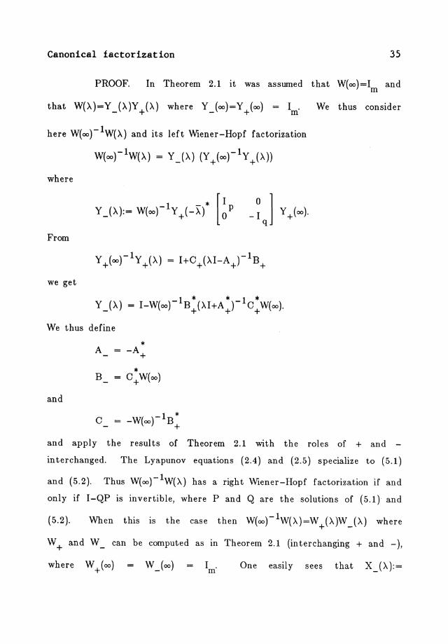
PROOF. In Theorem 2.1 it was assumed that W(oo) =1 and m
that W(A)=Y JA)Y +(A) where Y Joo)=Y +(00) = 1m' We thus consider
here W(oo)-lW(A) and its left Wiener-Hopf factorization
where
From
we get
We thus define
* A -A +
B
and
c
and apply the results of Theorem 2.1 with the roles of + and -
interchanged. The Lyapunov equations (2.4) and (2.5) specialize to (5.1)
and (5.2). Thus W(oo)-lW(A) has a right Wiener-Hopf factorization if and
only if I-QP is invertible, where P and Q are the solutions of (5.1) and
(5.2). When this is the case then W(oo)-lW(A)=W +(A)W _(A) where
W + and W _ can be computed as in Theorem 2.1 (interchanging + and -),
where W +(00) = W joo) I . m
One easily sees that XjA):=
36 Ball and Ran
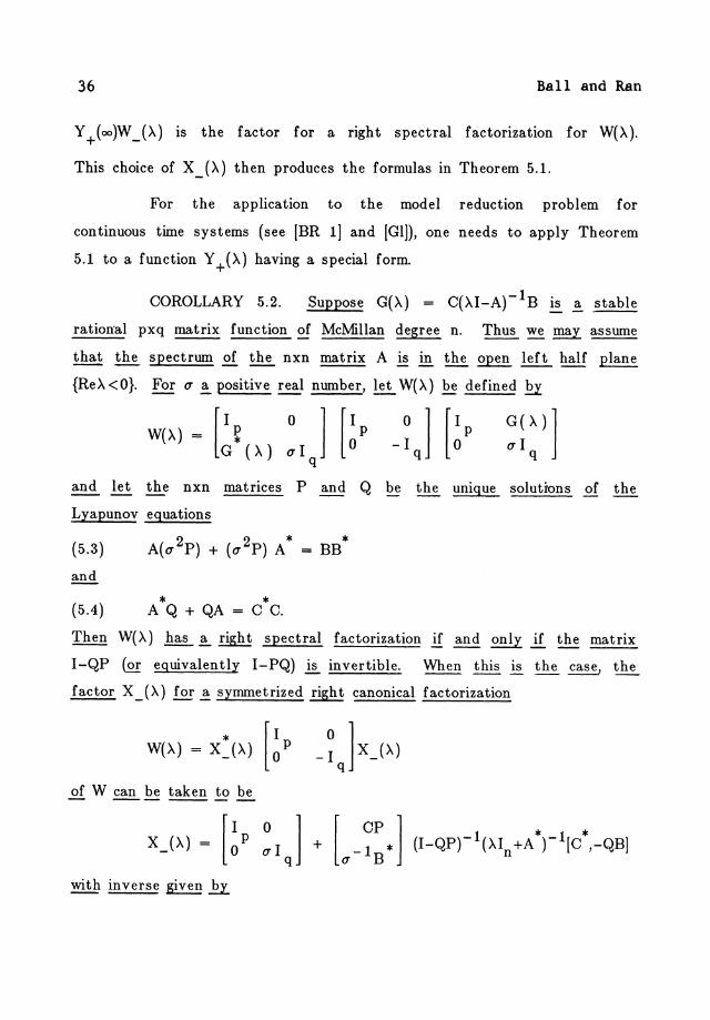
Y + (oo)W jA) IS the factor for a right spectral factorization for W(A).
This choice of X _(A) then produces the formulas in Theorem 5.1.
For the application to the model reduction problem for
continuous time systems (see [BR 11 and [GIl), one needs to apply Theorem
5.1 to a function Y +(A) having a special form.
COROLLARY 5.2. Suppose G(A) = C(AI-A)-l B is ~ stable
ration·al pxq matrix function of Mc:Millan degree n. Thus we may assume
that the spectrum of the nxn matrix A is in the open left half plane
{ReA<O}. For a ~ positive real number, let W(A) be defined £I
W( A) = [I f 0 1 [I p G (A) aI 0
q
and ~ the nxn matrices P and Q
Lyapunov equations
(5.3) 2 2 * * A(a P) + (a P) A = BB
and
* * (5.4) A Q + QA C C.
be the unique solutions of the
Then W(A) has ~ right spectral factorization if and only if the matrix
I-QP (Q! equivalently I-PQ) ~ invertible. When this is the case, the
factor X_(A) for ~ symmetrized right canonical factorization
of W can be taken to be
with inverse given .E.l:.
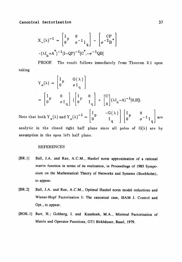
Canonical factorization 37
X_(A)-l ~ [~p ~-lIJ - [u-~:'l . (AI +A *)-I(I_QP)-I[C*,_u -IQBj
n
PROOF. The result follows inunediately from Theorem 3.1 upon
taking
1 [I Note that both Y +(A) and Y +(A)- = 0 p
analytic in the closed right half plane since all poles of G( A) are by
assumption in the open left half plane.
REFERENCES
[BR.I] Ball, J.A. and Ran, A.C.M., Hankel norm approximation of a rational
matrix function in terms of its realization, in Proceedings of 1985 Sympo-
sium on the Mathematical Theory of Networks and Systems (Stockholm),
to appear.
[BR.2] Ball, J.A. and Ran, A.C.M., Optimal Hankel norm model reductions and
Wiener-Hopf Factorization I: The canonical case, SIAM J. Control and
Opt., to appear.
[BGK.l] Bart, H.; Gohberg, I. and Kaashoek, M.A., Minimal Factorization of
Matrix and Operator Functions, OTI Birkhiiuser, Basel, 1979.
38 Ball and Ran
[BGK.2] Bart, H.; Gohberg, I. and Kaashoek, M.A., The coupling method for solv
ing integral equations, in Topics in Operator Theory Systems and Networks
(ed. H. Dym and I. Gohberg), OT 12 Birkhauser, Basel, 1983, 39-73.
[BGKvD] Bart, H.; Gohberg, I.; Kaashoek, M.A. and van Dooren, P., Factorization
of transfer functions, SIAM l. Control and Opt. 18 (1980), 675-696.
[CG] Clancey, K. and Gohberg, I., Factorization of Matrix Functions and Singu
lar Integral Operators, OT3 Birkhiiuser, Basel, 1981.
[Gl] Glover, K., All optimal Hankel-norm approximations of linear multivari
able systems and their V°-error bounds, Int. l. Control 39 (1984), 1115-
1193.
[GF] Gohberg, I.C. and Feldman, LA., Convolution Equations and Projection
Methods for their Solutions, Amer. Math. Soc. (Providence), 1974.
[GK] Gohberg, I.C. and Krupnik, N.la., Einfuhrung in die Theorie der eindi
mensionalen singuliiren Integraloperatoren, Birkhiiuser, Basel, 1979.
[H] Helton, J. W ., A spectral factorization approach to the distributed stable
regulator p'roblem: the algebraic Riccati equation, SIAM J. Control and
Opt. 14 (1976), 639-661.
[W] Willems, J., Least squares stationary optimal control and the algebraic Ric-
cati equation, IEEE Trans. Aut. Control AC-16 (1971),621-634.
J.A. Ball Department of Mathematics Virginia Tech Blacksburg, VA 24061 USA
A.C.M Ran Subfaculteit cler Wiskunde en Informatica Vrije Universiteit 1007 Me Amsterdam The Netherlands