modal scattering at an impedance transition in a … · modal scattering at an impedance transition...

Modal Scattering at an Impedance Transitionin a Lined Flow Duct

Sjoerd W. Rienstra∗Eindhoven University of Technology, 5600 MB Eindhoven, The Netherlands.

Nigel Peake†

University of Cambridge, Cambridge CB3 0WA, UK.

An explicit Wiener-Hopf solution is derived to describe the scattering of duct modes at a hard-soft wallimpedance transition in a circular duct with uniform mean flow. Specifically, we have a circular duct r =1,−∞ < x < ∞ with mean flow Mach number M > 0 and a hard wall along x < 0 and a wall of impedanceZ along x > 0. A minimum edge condition at x = 0 requires a continuous wall streamline r = 1 + h(x, t), nomore singular than h = O(x1/2) for x ↓ 0.

A mode, incident from x < 0, scatters at x = 0 into a series of reflected modes and a series of transmittedmodes. Of particular interest is the role of a possible instability along the lined wall in combination with theedge singularity. If one of the “upstream” running modes is to be interpreted as a downstream-running insta-bility, we have an extra degree of freedom in the Wiener-Hopf analysis that can be resolved by application ofsome form of Kutta condition at x = 0, for example a more stringent edge condition where h = O(x3/2) atthe downstream side. The question of the instability requires an investigation of the modes in the complex fre-quency plane and therefore depends on the chosen impedance model, since Z = Z(ω) is essentially frequencydependent.

The usual causality condition by Briggs and Bers appears to be not applicable here because it requires atemporal growth rate bounded for all real axial wave numbers. The alternative Crighton-Leppington criterion,however, is applicable and confirms that the suspected mode is usually unstable.

In general, the effect of this Kutta condition is significant, but it is particularly large for the plane waveat low frequencies and should therefore be easily measurable. For ω → 0, the modulus tends to |R001| →(1 + M)/(1 − M) without and to 1 with Kutta condition, while the end correction tends to ∞ without and to afinite value with Kutta condition. This is exactly the same behaviour as found for reflection at a pipe exit withflow, irrespective if this is uniform or jet flow.

Nomenclature

E = entire function, viz. a constantJm = ordinary Bessel function of the first kinds of order mh = perturbed position wall streamlinem = circumferential modal wave numberM = Mach numberµ, ν = radial modal ordern = unit outer normal vectors at r = 1v, p, ρ, c, φ = time-harmonic velocity, pressure, density, sound speed, potential perturbationsx , r , θ , t = axial, radial, azimuthal angle, time coordinateex , er , eθ = unit vectors in x , r , θ -directionαmν = radial modal wave numberγ = reduced radial wave numberκ = axial wave number

∗Associate Professor, Department of Mathematics & Computer Science, Eindhoven University of Technology, P.O. Box 513, 5600 MB Eind-hoven, The Netherlands. AIAA Member.

†Professor, Department of Applied Mathematics & Theoretical Physics, University of Cambridge, Centre for Mathematical Sciences, Wilber-force Road, Cambridge CB3 0WA, United Kingdom. AIAA member.

1 of 19

American Institute of Aeronautics and Astronautics

σ = reduced axial wave numberσmν , = reduced axial modal wave number hard-wall ductτmν , = axial modal wave number soft-wall ductψ = scattered potentialω = angular frequency; Helmholtz number� = reduced frequency

I. Introduction

SOUND transmission through a lined flow duct may be described by a sum of modes if geometry, lining and meanflow are independent of the axial coordinate. Mathematically, modes (in some cases including a continuous spec-

trum) form a complete basis for the representation of the sound field, but physically, they are each also (self-similar)solutions of the equations. Therefore, they provide much insight into the physical behaviour of the sound propagation.Most of our knowledge of duct acoustics is based on understanding the modes.

The modes in lined circular ducts with uniform mean flow are nearly completely understood.1 With hard wallswe have a finite number of cut-on (axially propagating) and infinitely many cut-off (axially exponentially decaying)modes. With soft walls this difference is slightly blurred; all modes decay exponentially but some are weakly cut-offwhile the others are heavily cut-off. Apart from this difference in axial direction, there is also a marked difference inthe cross-wise (radial) direction. Most modes are present throughout the duct, but some exist only near the wall. Theydecay exponentially in the radial direction away from the wall. These modes are called surface waves. Some exist bothwith and without flow, but some only with mean flow (of either type at most 2 per circumferential order for a hollowduct, 4 for an annular duct). The ones that exist only with mean flow are thus called hydrodynamic surface waves.1

By analogy with the Helmholtz instability along an interface between two media of different velocities, it wasrecognised by Ffowcs Williams and Tester2 that one such hydrodynamic surface wave may have the character of aninstability. This means that the mode seems to propagate in the upstream direction while it decays exponentially, but inreality its direction of propagation is downstream and it increases exponentially. Tester2 verified this conjecture by thecausality argument of Briggs and Bers3–5 (using physically reasonable frequency dependent impedance models) andfound that the suspected surface wave indeed may be an instability, at least according to the Briggs-Bers formalism.This was confirmed analytically by Rienstra in [1] for an incompressible limit of waves along an impedance of mass-spring-damper type, but now using the related causality criterion of Cright & Leppington.12, 26

Extending these ideas, Koch and Möhring6 analysed by a generalised Wiener-Hopf solution the scattered soundfield in a 2D duct with mean flow and a finite lined section. Their (Briggs-Bers) causality analysis was slightlyincomplete because they considered only frequency independent impedances, but otherwise they found results similarto Tester. If there is no instability wave available, the liner’s leading edge singularity could be no less than ratherstrong. If there is an instability this singularity can be weak, similar to the Kutta condition for a trailing edgea. Thesingularity at the liner’s trailing edge is more difficult to model9, 10 (the proper modelling may well be a nonlinear oneand involve essentially a finite thickness mean flow boundary layer) and the scattering by this edge may add a certainamount of uncertainty to the results. This, however, is greatly overshadowed by the fact that the field obtained in thelined section becomes exponentially large when the instability is included. This is in the greatest contrast with anyexperimental evidence, apart from some weak indication reported by Ffowcs Williams.11

It is therefore still an open question if these modes are really unstable, or maybe essentially nonlinear for anyreasonable acoustic amplitude because of the very high amplification rate.

On the other hand, this is not very unlike the situation for the jet. In agreement with theory, an instability indeedemerges from the exit edge, but further downstream the predicted Helmholtz instability is much less than is observed,because it quickly reaches the nonlinear regime. Still the major predicted acoustic consequences due to the excitationof the instability are very well described by linear theory12–25 and it makes sense to investigate a common situation.

In the jet exit problem we know that the instability may be excited by vortex shedding from a sharp edge. In theinviscid models we are dealing with, the vortex shedding is enforced by application of the Kutta condition.7, 23 Byanalogy we propose here the canonical problem of a duct, consisting of a semi-infinite hard-walled section and a semi-infinite lined section, with a mean flow that runs from the hard-walled to the soft-walled parts. The liner instability,if available, will be excited by application of some form of Kutta condition. Rather than the Briggs-Bers criterion

aThis Kutta condition essentially results from a delicate balance between viscous effects, nonlinear inertia and acceleration, described by a formof triple deck theory.7,8 It would be of interest to investigate if any consistent high-Reynolds triple deck or otherwise structure is possible that iscompatible with an absent instability and no Kutta condition.

2 of 19


(BB) we will use the Crighton-Leppington12, 26 causality test (CL), because, as we will show, BB is not applicablehere, while it gives sometimes different answers than CL. In the cases considered, the suspected mode is more oftendetected as an instability by CL than by BB.

Similar problems were proposed for the semi-infinite 2D problems27, 28 and for the 2D duct with a finite linedsection.6 Unfortunately, in all these cases the acoustically detectable difference between the situation with and withoutan instability is relatively small and experimental verification seems difficult. We will show that in the low Helmholtznumber limit of a circular duct there results a very large acoustical difference between presence and absence of theinstability. In similar problems for the exhaust jet it has been shown experimentally that the excitation of an instabilityis really physical and the effect on the acoustics is just as big as the theory predicts.16, 18–21

Although the present problem might be solved for most practical engineering purposes in a satisfactory way bymode matching, this method is not useful here as it provides no control of the edge singularity other than a posterioriby checking the convergence rate of the modal amplitudes. A much better approach in this respect is the Wiener-Hopftechnique.29 The problem of sound scattered in a semi-infinite duct is very apt to be treated by this method, while theedge singularity plays a most prominent role via the order of a polynomial function.

The pioneering Wiener-Hopf solution by Heins & Feshbach30 without flow is almost as classical as the relatedproblem for the unflanged pipe exit by Levine & Schwinger,31 but we will not follow their approach. To include flowand Kutta condition in a convenient way, we will use a 3D version of the 2D analysis outlined in [28].

II. The problem

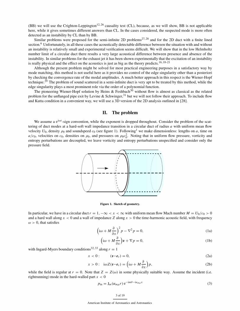
We assume a eiωt -sign convention, while the exponent is dropped throughout. Consider the problem of the scat-tering of duct modes at a hard-soft wall impedance transition in a circular duct of radius a with uniform mean flowvelocity U0, density ρ0 and soundspeed c0 (see figure 1). Following1 we make dimensionless: lengths on a, time ona/c0, velocities on c0, densities on ρ0, and pressures on ρ0c2

0. Noting that in uniform flow pressure, vorticity andentropy perturbations are decoupled, we leave vorticity and entropy perturbations unspecified and consider only thepressure field.

Figure 1. Sketch of geometry.

In particular, we have in a circular duct r = 1,−∞ < x < ∞ with uniform mean flow Mach number M = U0/c0 > 0and a hard wall along x < 0 and a wall of impedance Z along x > 0 the time-harmonic acoustic field, with frequencyω > 0, that satisfies (

iω + M∂

∂x

)2p − ∇2 p = 0, (1a)(

iω + M∂

∂x

)v + ∇ p = 0, (1b)

with Ingard-Myers boundary conditions32, 33 along r = 1

x < 0 : (v· er ) = 0, (2a)

x > 0 : iωZ(v· er ) =(

iω + M∂

∂x

)p, (2b)

while the field is regular at r = 0. Note that Z = Z(ω) in some physically suitable way. Assume the incident (i.e.rightrunning) mode in the hard-walled part x < 0

pin = Jm(αmµr) e−imθ−iκmµx (3)

3 of 19


where m ≥ 0, Jm is the m-th order ordinary Besselfunction of the first kind34. −α2mµ is an eigenvalue of the Laplace

operator in a circular cross section with Neumann boundary conditions, and given by

α1−mmµ J′

m(αmµ) = 0, (4)

i.e. the non-trivial zeros of J′m . αmµ is usually called the radial modal wave number. The axial modal wave number

κmµ is defined through the dispersion relation

α2mµ + κ2

mµ = (ω − Mκmµ)2 (5)

such that the branch is taken with Re(κmµ) > 0 if the mode is cut-on or Im(κmµ) < 0 if the mode is cut-off. Due tocircumferential symmetry, the scattered wave will depend on θ via e−imθ only, and we will from here on assume thatp := p e−imθ where the exponent will be dropped.

After introducing the velocity potential with v = ∇φ, we can integrate (1b) to get

(iω + M

∂

∂x

)φ + p = 0. (6)

(The integration constant is not important.) So we have for the corresponding incident mode

φin = i

ω − Mκmµpin. (7)

We introduce the scattered part ψ of the potential by

φ = φin + ψ. (8)

It is convenient to reformulate the boundary condition by way of the wall stream line given by

r = 1 + Re(h(x) eiωt−imθ). (9)

We have then at r = 1 (note that ∂∂r φin = 0 at r = 1)

∂ψ

∂r= 0 for x < 0, (10a)

∂ψ

∂r=

(iω + M

∂

∂x

)h for x > 0, (10b)

p = iωZh for x > 0. (10c)

We expect some singular behaviour at x = 0, but no more than what goes together with a continuous wall streamline,so h(0) = 0 and h(x+) ≤ O(xη) for a η > 0.

III. The Wiener-Hopf analysis

We introduce the Fourier transforms to x

ψ̂(κ, r) =∫ ∞

−∞ψ(x, r) eiκx dx, (11a)

H+(κ) =∫ ∞

0h(x) eiκx dx, (11b)

P−(κ) =∫ 0

−∞

(iω + M

∂

∂x

)ψ(x, 1) eiκx dx, (11c)

to obtain for ψ̂ the Bessel-type equation

∂2ψ̂

∂r2 + 1

r

∂ψ̂

∂r+

[(ω − Mκ)2 − κ2 − m2

r2

]ψ̂ = 0. (12)

4 of 19


We introduce the reduced frequency�, Fourier wavenumber σ and radial wave number γ as follows.

β =√

1 − M2, ω = β�, κ = �

β(σ − M)

�γ =√(ω − Mκ)2 − κ2 = �

√1 − σ 2, γ =

√1 − σ 2 where Im(γ ) ≤ 0.

(13)

With (10a), (10b) and (11b) we arrive at the solution

ψ̂ = A(σ ) Jm(�γ r), (14a)

A(σ ) = i1 − Mσ

βγ J′m(�γ )

H+. (14b)

Since (iω + M

∂

∂x

)ψ = pin − p, (15)

we have along the wall r = 1

i(ω − Mκ)A Jm(�γ ) = P− +∫ ∞

0pin eiκx dx −

∫ ∞

0p eiκx dx, (16)

which reduces to

i(ω − Mκ)A Jm(�γ ) = P− + i Jm(αmµ)

κ − κmµ− iωZ H+, (17)

and

− �

β2 (1 − Mσ)2Jm(�γ )

γ J′m(�γ )

H+ + iβ�Z H+ = P− + iβ Jm(αmµ)

�(σ − σmµ)(18)

where we introduced

σmµ =√

1 − α2mµ

�2, (19)

such that Re(σmµ) > 0 and Im(σmµ) = 0, or Im(σmµ) < 0. This yields

P−(σ )+ iβ Jm(αmµ)

�(σ − σmµ)= −K (σ )H+(σ ), (20)

where the Wiener-Hopf kernel K is defined by

K (σ ) = �

β2(1 − Mσ)2

Jm(�γ )

γ J′m(�γ )

− iβ�Z (21)

Note that Jm(�γ )/�γ J′m(�γ ) is a meromorphic function of �2γ 2 and therefore of σ 2. So K is a meromorphic

function of σ with isolated poles and zeros. The zeros, corresponding with the reduced axial wave numbers in thelined part of the duct, are given by

χ(σ) = (1 − Mσ)2 Jm(�γ )− iβ3 Zγ J′m(�γ ) = 0 (22)

denoted by σ = τmν , ν = 1, 2, . . . , for the rightrunning modes of the lower complex half plane (see figure 2). Theonly possible candidate of a rightrunning mode from the upper-half plane (which then has to be an instability) will bedenoted (following [1]) by σ = σH I , where the subscript refers to ”hydrodynamic instability” (a possible example isfound in the upper right corner of figure 2). The poles, corresponding with the reduced axial wave numbers in the hardpart of the duct, are given by

γ 1−m J′m(�γ ) = 0, (23)

denoted by σ = σmν , implicitly given by �γ = αmν , ν = 1, 2, . . . where αmν denote the non-trivial zeros of J′m . For

hard-walled ducts, the left and right running reduced wave numbers are symmetric, and so the left-running hard-wallmodes are given by σ = −σmν .

5 of 19


−2 0 2 4 6 8 10−4

−3

−2

−1

0

1

2

3

4

Figure 2. Typical location of soft-wall wave numbers τmν (indicated by ◦) and hard-wall wave numbers σmν (indicated by ×). Note the 3soft-wall surface waves. (Z = 0.8 − 2i, ω = 10,M = 0.5,m = 0.)

In the usual way29 we split K into functions that are analytic in the upper and in the lower half plane (but note apossible instability pole in the upper half plane that really is to be counted to the lower half plane; see below)

K (σ ) = K+(σ )K−(σ )

. (24)

Following appendix A, we introduce the auxiliary split functions N+ and N−, satisfying

K (σ ) = N+(σ )N−(σ )

(25)

and given by

log N±(σ ) = 1

2π i

∫ ∞

0

[ln K (u)

u − σ− ln K (−u)

u + σ

]du. (26)

The + sign corresponds with Im σ > 0 or Im σ = 0 & Re σ < 0, and the − sign with Im σ < 0 or Im σ =0 & Re σ > 0. (Use for points from the opposite side the definition K N− = N+.) Following appendix A, we obtainthe following asymptotic behaviour

N±(σ ) = O(σ±1/2). (27)

When no instability pole crossed the contour, we identify

K+(σ ) = N+(σ ), K−(σ ) = N−(σ ). (28)

When an instability pole σH I crossed the contour and is to be included among the right-running modes of the lowerhalf-plane, N− contains the factor (σ − σH I )

−1, so the causal split functions are

K+(σ ) = (σ − σH I )N+(σ ), K−(σ ) = (σ − σH I )N−(σ ). (29)

We continue with our analysis. We substitute the split functions in equation (20) to get

K−(σ )P−(σ )+ iβ Jm(αmµ)K−(σ )− K−(σmµ)

�(σ − σmµ)= −K+(σ )H+(σ )−

iβ Jm(αmµ)K−(σmµ)

�(σ − σmµ)(30)

The left hand side is a function analytic in the lower halfplane, while the right hand side is analytic in the upperhalfplane. So together they define an entire function E .

From the estimate h(x) = O(xη) for x ↓ 0 and η > 0, it follows [29, page 36] that

H+(σ ) = O(σ−η−1) (σ → ∞). (31)

6 of 19


This gives us the information to determine E . If there is no instability pole, then K+(σ )H+(σ ) = O(σ−η−1/2), and soE vanishes at infinity and has to vanish everywhere according to Liouville’s theorem.29 If there is an instability pole,we have an extra factor σ and so K+(σ )H+(σ ) = O(σ−η+1/2). This means that if η = 1/2 (no smooth streamline atx = 0, i.e. no Kutta condition), the entire function is only bounded and equal to a constant. If unmodelled physicaleffects (nonlinearities, viscosity) requires a smooth behaviour of h near x = 0, i.e. the Kutta condition, we have tochoose E = 0, as this yields η = 3/2. See figure 3.

(a) no Kutta condition, no instability (b) no Kutta condition, instability (c) Kutta condition, instability

Figure 3. Types of edge singularity. Note that in the Ingard-Myers model the perturbed wall stream line does not cross the wall. It ispositioned slightly off the wall at a distance, small compared to a wave length but large compared to any acoustic perturbation.

We will start with the assumption of an instability pole. As we will see, the other case will be automaticallyincluded in the formulas, and it will not be necessary to consider both cases separately.

We scale the constant E

E = −iβ Jm(αmµ)K−(σmµ)

�(σH I − σmµ)(1 − �) = − iβ

�Jm(αmµ)N−(σmµ)(1 − �) (32)

such that � = 0 corresponds with no excitation of the instability (no contribution from σH I ), while � = 1 correspondswith the full Kutta condition. Anything inbetween will correspond to a certain amount of instability wave, but notenough to produce a smooth solution in x = 0. It is readily verified that the assumption of no instability pole, i.e.K+ = N+ and E = 0, leads to exactly the same formula as with � = 0. So in the following we will identify withcondition � = 0 both the situation of no instability pole as well as the situation of an instability that is (for whateverreason) not excited.

The total solution is now given by the following inverse Fourier integral, with a deformation around the poleσ = σH I if � = 0. (This deformation will result in a residue contribution if x > 0.)

p = pin +�

2π iβ2 Jm(αmµ)N−(σmµ)

∫ ∞

−∞∩ (1 − Mσ)2 Jm(�γ r)

γ J′m(�γ )N+(σ )

[1

σ − σmµ− �

σ − σH I

]exp

(i�

β(M − σ)x

)dσ (33)

For x < 0 we close the contour around the lower complex half-plane, and sum over the residues of the poles inσ = −σmν , the axial wave numbers of the left-running hard-walled modes. We obtain the field

p = pin +∞∑ν=1

Rmµν Jm(αmν) exp(

i�

β(M + σmν)x

)(34)

where

Rmµν = Jm(αmµ)N−(σmµ)(1 + Mσmν )2

β2σmν

(1 − m2

α2mν

)Jm(αmν)N+(−σmν)

[1

σmν + σmµ− �

σmν + σH I

](35)

In particular

R011 = 1 + M

1 − M

N−(1)N+(−1)

[1

2− �

1 + σH I

](36)

7 of 19


For the transmitted field in x > 0 we close the contour around the upper half-plane and sum over the residuesfrom σ = τmν , σmµ and (if � = 0) σ = σH I . We note that the residue from σ = σmµ just cancels pin , while the otherresidues (except from σH I ) are found after rewriting (cf. equation (22))

γ J′m(�γ )N+(σ ) = �

β2χ(σ)N−(σ ). (37)

We obtain

p =∞∑ν=1

Tmµν Jm(βmνr) exp(

i�

β(M − τmν)x

)

− ��2

β2 Jm(αmµ)N−(σmµ)(1 − MσH I )

2

βH I J′m(βH I )N+(σH I )

Jm(βH I r) exp(

i�

β(M − σH I )x

)(38)

where βmν = �γ (τmν), βH I = �γ (σH I ), and

Tmµν = −β Jm(αmµ)N−(σmµ)(1 − Mτmν )2

χ ′(τmν)N−(τmν)

[1

τmν − σmµ− �

τmν − σH I

], (39)

while χ ′(τmν) can be further specified to be

χ ′(τmν) = −iβ2 Z Jm(βmν)

[ωτmν

(1 − m2

β2mν

− �4mν

(ωβmν Z)2

)− 2iM�mν

ωZ

], �mν = ω(1 − Mτmν)

β2. (40)

(This expression may be compared with (16) of [35].)

IV. Causality

To determine the direction of propagation of the modes, and thus detect any possible instability, we have availablethe following causality criteria:

• The Briggs-Bers3–5 formalism, where analyticity in the whole lower complexω-plane is enforced by tracing thepoles for fixed Re(ω), and Im(ω) running from 0 to −∞.

• The Crighton-Leppington12, 26 formalism, where analyticity in the whole lower complex ω-plane is enforced bytracing the poles for fixed |ω|, and arg(ω) running from 0 to − 1

2π .

Interestingly, these two methods give conflicting results as to the existence or otherwise of instability waves, and infact it turns out that it is only the Crighton & Leppington approach which can be applied in this case. However, sincethe Briggs-Bers method is in common use we will first describe its predictions in some detail, before explaining whyit is actually inapplicable here. We will then present the results from the (legitimate) application of the Crighton &Leppington procedure.

For definiteness we will model the complex, frequency-dependent impedance as a simple mass-spring-dampersystem

Z(ω) = R + iaω − ib

ω, (41)

which satisfies the fundamental requirements for Z to be physical and passive (see e.g. [36]), viz. Z is analytic andnon-zero in Im(ω) < 0, Z(ω) = Z∗(−ω) and Re(Z) > 0. We will briefly consider another possible model at the endof this section.

Turning first to the Briggs-Bers method, sample results are presented on the left of figures 4 & 5. Note that infigure 4 the instability wave starts in the first quadrant of the κ plane, but then crosses the real axis as Im(ω) → −∞.The Briggs-Bers method therefore predicts that this mode propagates downstream (i.e. its group velocity points in thedownstream direction) and that it is unstable. In contrast, note that in figure 5 the surface mode remains above the κaxis as Im(ω) → −∞, so that the Briggs-Bers method predicts that this mode propagates in the upstream directionand decays. It is straightforward to derive a criterion to distinguish between these two different cases, by consideringthe behaviour of the corresponding root of the dispersion relation (22) as Im(ω) → −∞. We write

σ = Im(ω)σ0 + σ1 + O(Im(ω)−1), (42)

8 of 19


and then note that

γJ′

m(�γ )

Jm(�γ )∼ Im(ω)σ0 + σ1 + O(Im(ω)−1). (43)

Substituting this result into (22) and equating powers of Im(ω), we find an expansion for the surface-wave modenumber in the form

κ = Im(ω)2aβ

M2− Im(ω)Rβ

M2+ i

Im(ω)

β2 M2

[M(2 − M2)− 2aβ3 Re(ω)

] + . . . . (44)

From this expression we can see straightaway that in the Briggs-Bers method instability will be predicted (i.e. the modeapproaches infinity through the lower half of the κ plane as Im(ω) → −∞) if and only if M(2− M2)/2β3 Re(ω) > a,and this condition exactly matches the behaviour seen in figures 4 & 5. Note that in figure 5(b) the critical value of afor instability is a = 0.1451, compared to the value a = 0.15 used in the computation, explaining why the trajectoryof the mode is almost parallel to the real κ axis.

−30 −20 −10 0 10 20 30 40

−30

−20

−10

0

10

20

30

−8 −6 −4 −2 0 2 4 6 8

−30

−20

−10

0

10

20

30

Figure 4. Causality contours for complex ω according to the Briggs-Bers (left) and the Crighton-Leppington (right) formalism. The crossesindicate the location of the modes when Im(ω) = 0. Both criteria agree in their conclusion about the instability. (Z = 1 − 0.9i, ω = 1,M =0.5,m = 0, a = 0.1, b = 1.)

Unfortunately, the Briggs-Bers predictions described in the previous paragraph cannot be applied to our real prob-lem. This is because there is a rather subtle, but crucial, technical condition which needs to be satisfied before theBriggs-Bers method can be used. What is required is that the system has a finitely-bounded temporal growth rate forall real κ , which allows the temporal inversion contour to be located sufficient low in the complex ω plane so as to liebelow all singularities in the ω Fourier transform. To be completely specific, consider the linear system

D

(i∂

∂ t,−i

∂

∂xφ

)= F(t)δ(x), (45)

where D is a linear operator and F(t) is the forcing such that F(t) = 0 for t < 0. Fourier transforming in t and x andinverting, we find the solution

φ(x, t) = 1

4π2

∫C

∫ ∞

κ=−∞F (ω)

D(κ, ω)eiωt−iκx dκdω. (46)

In order to have the causal response φ = 0 when t < 0 we need to choose the temporal inversion contour C to liebelow the singularities (in ω-domain) of

φ (x, ω) = 1

2πF (ω)

∫ ∞

κ=−∞e−iκx

D(κ, ω)dκ (47)

Since F(t) < 0 for t < 0, it follows that its Fourier transform, F (ω), is analytic in the lower half plane, so thatnon-analytic behaviour (in ω) of φ (x, ω) would arise from any singularity of the integrand κn(ω), i.e. given byD(κ, ω) = 0, crossing the real κ-axis for some ω ∈ C. Hence we need to choose C such that for any κn

Im(κn(ω)) = 0 for all ω ∈ C. (48)

9 of 19


0 50 100 150 200 250−60

−40

−20

0

20

40

60

80

100

120

140

−20 0 20 40 60 80

−60

−40

−20

0

20

40

60

80

(a) Z = 1 + 3.335i, ω = 10,M = 0.7,m = 0, a = 0.335, b = 0.15

0 50 100 150 200−40

−30

−20

−10

0

10

20

30

40

50

60

−40 −20 0 20 40 60−40

−30

−20

−10

0

10

20

30

40

50

60

(b) Z = 1 + 1.385i, ω = 10, M = 0.7,m = 5, a = 0.15, b = 1.15

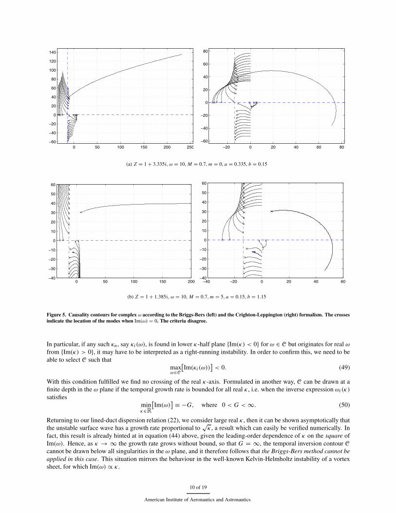
Figure 5. Causality contours for complex ω according to the Briggs-Bers (left) and the Crighton-Leppington (right) formalism. The crossesindicate the location of the modes when Im(ω) = 0. The criteria disagree.

In particular, if any such κn , say κi (ω), is found in lower κ-half plane {Im(κ) < 0} for ω ∈ C but originates for real ωfrom {Im(κ) > 0}, it may have to be interpreted as a right-running instability. In order to confirm this, we need to beable to select C such that

maxω∈C

[Im(κi (ω))

]< 0. (49)

With this condition fulfilled we find no crossing of the real κ-axis. Formulated in another way, C can be drawn at afinite depth in the ω plane if the temporal growth rate is bounded for all real κ , i.e. when the inverse expression ωi (κ)

satisfiesminκ∈R

[Im(ω)

] ≡ −G, where 0 < G < ∞. (50)

Returning to our lined-duct dispersion relation (22), we consider large real κ , then it can be shown asymptotically thatthe unstable surface wave has a growth rate proportional to

√κ , a result which can easily be verified numerically. In

fact, this result is already hinted at in equation (44) above, given the leading-order dependence of κ on the square ofIm(ω). Hence, as κ → ∞ the growth rate grows without bound, so that G = ∞, the temporal inversion contour Ccannot be drawn below all singularities in the ω plane, and it therefore follows that the Briggs-Bers method cannot beapplied in this case. This situation mirrors the behaviour in the well-known Kelvin-Helmholtz instability of a vortexsheet, for which Im(ω) ∝ κ .

10 of 19


Having decided that the Briggs-Bers method cannot be applied, we now turn to the procedure of Crighton &Leppington.12, 26 The analysis described in [12] concerns the causal solution for scattering of acoustic waves by asemi-infinite vortex sheet, and in many ways can therefore be thought of as being analogous to problem considered inthe present paper. Specifically, the difficulty associated with the unbounded growth rate of the vortex sheet is handledin [12,26] by first supposing that the argument of ω is close to (with the present sign convention) − 1

2π . This approachis guaranteed to yield a causal result, since the solution then decays to zero as t → −∞. Once the Fourier transformhas been determined with imaginary ω, the idea is then to attempt to analytically continue the Fourier transform backto the physically-relevant case of real ω. So we set

ω = |ω| exp(iϕ), (51)

and allow ϕ to increase from − 12π to 0. As ϕ increases, the singularities in the Fourier transform will move in the κ

plane, and to retain analyticity we must deform the κ inversion contour so as to prevent any singularities crossing it.The singularities correspond to the κ roots of (22), and their motion in typical cases is shown in figures 4 and 5. Notethat in each case it is only the single surface wave which crosses the real κ axis, having started in the lower half ofthe κ plane when ϕ = − 1

2π . It therefore follows that, in order to avoid a pole crossing, the κ inversion contour mustbe deformed so as to run above this pole. This means that the surface wave is picked up when the spatial contour isclosed in the lower half plane for x > 0, and corresponds to a downstream instability. We can therefore conclude thatin each of the cases described in figures 4 & 5 the Crighton-Leppington method predicts that the system is unstable.

For the special case of a semi-infinite 2D half-space in the incompressible limit it was shown in [1] analytically thatthe system is unstable according to the Crighton-Leppington procedure. In general, however, it appears that in order touse this procedure to test the stability of our system we need to solve the dispersion relation numerically, tracking theprogress of the possible instability in the κ plane as ϕ is increased from − 1

2π to 0. Additional to the incompressiblelimit, we can make further algebraic progress for large values of Re(ω). In much the same way as for the Briggs-Bersmethod, we write

σ = |ω| exp(iϕ)σ0 + σ1 + O(|ω|−1), (52)

and after some algebra find that the unstable surface wave is given by

κ = −βa|ω|2M2

exp(2iϕ)+(

iβ3 R

M2+ 2

M− M

) |ω| exp(iϕ)

β2+ O(|ω|−1). (53)

We now follow the Crighton-Leppington procedure of increasing ϕ from − 12π to 0, and we see from (53) that Im(κ) <

0 when ϕ = − 12π (since M < 1) and Im(κ) > 0 when ϕ = 0 (since R > 0). This shows us that this mode has crossed

the real κ axis as ϕ is increased, so that it is indeed a genuine instability. Note that even if a = 0 the mode still crossesthe real κ axis, although in this case the typical spatial growth rates are rather smaller, scaling on |ω| rather than |ω2|.

In summary, we can conclude that our system is genuinely unstable for the situations described in figures 4 & 5,as well as in the limit of large real frequency. It should be noted, however, that this conclusion may be dependent onthe functional dependence of Z on ω, and different impedance models need to be studied on a case-by-case basis. Wedo note that for another common case, the Helmholtz-resonator model, the conclusion of instability at large Re(ω) isalso obtained. Writing (for positive constants m and L)

Z = R + imω − i cot(ωL), (54)

and noting that cot z → i as z → ∞ with Im(z) < 0, we see that the large-Re(ω) expansion for the wavenumber isagain given by (53), but with R replaced by R + 1. It then follows that the mode still crosses the real κ-axis as ϕ isincreased, so that the system is again unstable.

V. Low-frequency asymptotics

An interesting limit in the present context is the one for small ω. In this case only the reflection coefficient R011 ofthe plane wave is of interest. We have for small ω

K (σ ) = −2(1 − Mσ)2

β2γ (σ)2+ O(ω) (ω → 0). (55)

The double zeros σ = M−1 arise from two modes, one from the upper half plane and one from the lower half plane,that meet each other at ω = 0. These modes are of surface wave type1 because the radial wave number is purely

11 of 19


imaginary, but for low ω the radial decay is so slow that their confinement to the wall inside the duct is meaningless.The mode from the upper half plane is (in all cases considered) the instability σH I . The other one is in the nomenclatureof [1] the right-running acoustic surface wave σS R . In the present notation it is a mode from the set {τ0ν}, sayb, τ01 or(to avoid any ambiguity) τ+

01. For smal but non-zero ω they are asymptotically given by

σH I = M−1 + 12 (1 + i)β2 M−2

√ωZ + . . . (56a)

τ+01 = M−1 − 1

2 (1 + i)β2 M−2√ωZ + . . . (56b)

This is illustrated by figure 6. The first two left and right-running modes are drawn as a function of Z = 1 + iλ,where λ is varied from ∞ (hard wall) to −∞ (again hard wall). Starting as the right-running hard-wall plane waveσ01 = 1, τ+

01 becomes slightly complex, resides near M−1 when λ = 0, but returns to its starting hard-wall value whenλ → −∞. The second right-running mode τ+

02 (the first cut-off) disappears to real −∞. The left-running mode τ−01

starts as the hard-wall plane-wave mode −σ01 = −1, then moves to the right, resides near M−1 when λ = 0 (where itapparently has changed its character and has become a right-running instability wave !) and then, instead of returningto its original hard-wall value, it disappears to real +∞. Its position has been taken over by the second left-runningmode τ−

02.

−15 −10 −5 0 5 10 15 −35

−30 −25 −20 −15 −10 −5 0 5 10 15 20 25 30 35

τ−01, σH I

τ+01

τ−02

τ+02

(a) ω = 0.1,Re(Z) = 1,m = 0,M = 0.5

−2 −1 0 1 2 3 4 −1

−0.5

0

0.5

1

−σ01 σ01

τ−01, σH I

τ+01

τ−02

(b) ω = 0.01,Re(Z) = 1,m = 0,M = 0.5

Figure 6. Modal wave numbers τ±0ν as they traverse the complex σ -plane for varying impedance Z = 1 + iλ.

Now we can approximate the split functions

N+(σ ) � −21 − Mσ

β2(1 − σ), N−(σ ) � 1 + σ

1 − Mσ, (57)

not necessarily with the same multiplicative factor as would arise from representation (A.9). This yields for the planewave reflection coefficient

R011 � −1 + M

1 − M

(1 − 2M�

1 + M

)+ . . . (ω → 0), (58)

resulting in the remarkably different values R011 = −1 for � = 1 and R011 = −(1 + M)/(1 − M) for � = 0,irrespective of Z (although the limit Z → ∞, ω → 0 will be non-uniform). This result is exactly the same as foundfor the low frequency plane wave reflection coefficients of a semi-infinite duct with jet or uniform mean flow.14, 19–22

The instability wave corresponding to (56a), with axial wave number the Strouhal number ω/M , vanishes inpressure, due to the factor (1 − MσH I ), but survives in the potential or velocity. The transmission coefficient of the

bThere is no obvious way of sorting soft-wall modes; see figure 6.

12 of 19


wave corresponding to (56b), with the same axial wave number, appears to be

T011 � 12�

(1 + M

1 − M

)1/2 + . . . (59)

VI. Results

In order to illustrate the above results we have evaluated numerically (see Appendix A) the reflection coefficientsR011 of the plane wave mode mµ = 01 into itself as a function of frequency ω, and reflection coefficient R111 of themode mµ = 11 into itself. The impedance is rather arbitrarily picked as Z = 1 − 2i and the Mach number M = 0.5.Both modulus |R.11| and phase φ.11 are plot but for the lower frequencies the plane wave phase is reformulated to anend correction δ011, i.e. the virtual point beyond x = 0, scaled by ω, where the wave seems to reflect with condition|p| is minimal. Since ∣∣∣e−i ω

1+M x +R011 ei ω1−M x

∣∣∣2 = 1 + |R011|2 + 2|R011| cos(

2ω1−M2 x + φ011

)is minimal if 2ω

1−M2 x + φ011 = π , so

δ011 = (1 − M2)π − φ011

2ω. (60)

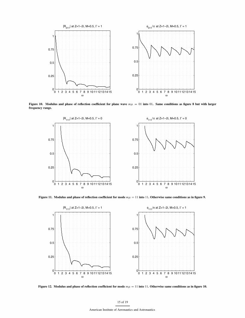
In order to facilitate comparison with the low ω-analysis, the results are both given for a small interval 0 ≤ ω ≤ 1 and alarge interval 0 ≤ ω ≤ 15. (The endcorrection is given only for the small interval because it loses its meaning for largerfrequencies.) The most striking result is probably the confirmation of the analytically found reflection coefficients 1(Kutta condition; figure 7 left) and (1 + M)/(1 − M) (no Kutta condition; figure 8 left) for ω → 0, and in additionthat the end correction tends to a finite value (Kutta condition; figure 7 right) and to ∞ (no Kutta condition; figure 8right). This is also in exact analogy with the jet.21 Note that this behaviour is not related to ω = 0 being a resonancefrequency because R111 tends to 1 at its first resonance frequency in both cases (figures 11 and 12).

VII. Conclusions

An explicit Wiener-Hopf solution is derived to describe the scattering of duct modes at a hard-soft wall impedancetransition at x = 0 in a circular duct with uniform mean flow. A mode, incident from the hard-walled upstream part,is scattered into reflected hard-wall and transmitted soft-wall modes. A plausible edge condition at x = 0 requires atleast a continuous wall streamline r = 1 + h(x, t), no more singular than h = O(x1/2) for x ↓ 0. By analogy witha trailing edge scattering problem, the possibility of vortex shedding from the hard-soft transition would allow us toapply the Kutta condition and require the edge condition to be no more singular than corresponding to h = O(x3/2)

for x ↓ 0.The physical relevance of this Kutta condition is still an open question. It all depends on the direction of prop-

agation of the soft-wall modes. The Wiener-Hopf analysis shows that no Kutta condition can be applied if none ofthe apparently up-stream running, decaying, soft-wall modes is in reality a downstream-running instability. However,causality analyses in the complex frequency domain, taking into account the frequency dependence of the impedance,indicate that under certain circumstances one soft-wall mode (per circumferential order) is to be considered as aninstability. In this cases we may be able to enforce a Kutta condition and thus excite the instability.

As the growth rate of this presumed instability may be very high, it remains to be seen if this result is an artefactof the linearised model or really representative of reality. There is apparently a need for clarifying and distinguishingexperiments to be carried out.

We presented the results for either cases (Kutta and no Kutta condition), and showed that the difference is, forcertain choices of parameters, big enough for experimental verification. In particular, the pressure reflection coefficientfor the plane wave in the low Helmholtz number regime is near unity for Kutta, and near (1 + M)/(1 − M) for the noKutta condition case.

A. Appendix

Split functions

The complex function K (σ ) has poles and zeros in the complex plane, in particular also along the real axis. We need toevaluate K , written as a quotient of two function that are analytic in upper and lower halfplane, along the real κ-axis.

13 of 19


0 0.1 0.2 0.3 0.4 0.5 0.6 0.7 0.8 0.9 10

0.25

0.5

0.75

1

1.25

1.5

1.75

2

2.25

2.5

2.75

3

ω

|R011

| at Z=1−2i, M=0.5, Γ = 0

0 0.1 0.2 0.3 0.4 0.5 0.6 0.7 0.8 0.9 10

0.25

0.5

0.75

1

1.25

1.5

1.75

2

2.25

2.5

ω

δ011

at Z=1−2i, M=0.5, Γ = 0

Figure 7. Modulus of reflection coefficient and end correction for plane wave mµ = 01 into 01, where plane wave is incident from hard-walled section to lined section with impedance Z = 1 − 2i, while M = 0.5. Without Kutta condition at x = 0.

0 0.1 0.2 0.3 0.4 0.5 0.6 0.7 0.8 0.9 10

0.25

0.5

0.75

1

ω

|R011

| at Z=1−2i, M=0.5, Γ = 1

0 0.1 0.2 0.3 0.4 0.5 0.6 0.7 0.8 0.9 10

0.1

0.2

0.3

0.4

0.5

ω

δ011

at Z=1−2i, M=0.5, Γ = 1

Figure 8. Modulus of reflection coefficient and end correction for plane wave mµ = 01 into 01, where plane wave is incident from hard-walled section to lined section with impedance Z = 1 − 2i, while M = 0.5. With Kutta condition at x = 0.

0 1 2 3 4 5 6 7 8 9 1011121314150

0.5

1

1.5

2

2.5

3

ω

|R011

| at Z=1−2i, M=0.5, Γ = 0

0 1 2 3 4 5 6 7 8 9 1011121314150

0.5

1

ω

φ011

/π at Z=1−2i, M=0.5, Γ = 0

Figure 9. Modulus and phase of reflection coefficient for plane wave mµ = 01 into 01. Same conditions as figure 7 but with larger frequencyrange.

14 of 19


0 1 2 3 4 5 6 7 8 9 1011121314150

0.25

0.5

0.75

1

ω

|R011

| at Z=1−2i, M=0.5, Γ = 1

0 1 2 3 4 5 6 7 8 9 1011121314150

0.25

0.5

0.75

1

ω

φ011

/π at Z=1−2i, M=0.5, Γ = 1

Figure 10. Modulus and phase of reflection coefficient for plane wave mµ = 01 into 01. Same conditions as figure 8 but with largerfrequency range.

0 1 2 3 4 5 6 7 8 9 1011121314150

0.25

0.5

0.75

1

ω

|R111

| at Z=1−2i, M=0.5, Γ = 0

0 1 2 3 4 5 6 7 8 9 1011121314150

0.25

0.5

0.75

1

ω

φ111

/π at Z=1−2i, M=0.5, Γ = 0

Figure 11. Modulus and phase of reflection coefficient for mode mµ = 11 into 11. Otherwise same conditions as in figure 9.

0 1 2 3 4 5 6 7 8 9 1011121314150

0.25

0.5

0.75

1

ω

|R111

| at Z=1−2i, M=0.5, Γ = 1

0 1 2 3 4 5 6 7 8 9 1011121314150

0.25

0.5

0.75

1

ω

φ111

/π at Z=1−2i, M=0.5, Γ = 1

Figure 12. Modulus and phase of reflection coefficient for mode mµ = 11 into 11. Otherwise same conditions as in figure 10.

15 of 19


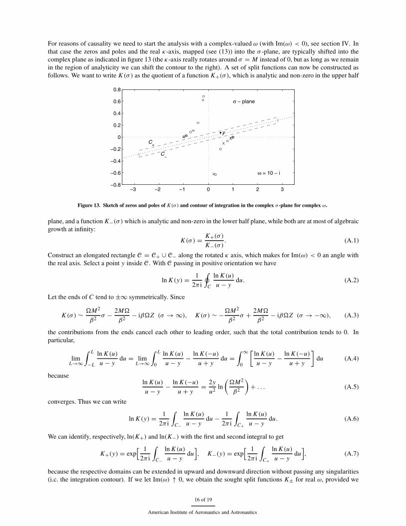
For reasons of causality we need to start the analysis with a complex-valued ω (with Im(ω) < 0), see section IV. Inthat case the zeros and poles and the real κ-axis, mapped (see (13)) into the σ -plane, are typically shifted into thecomplex plane as indicated in figure 13 (the κ-axis really rotates around σ = M instead of 0, but as long as we remainin the region of analyticity we can shift the contour to the right). A set of split functions can now be constructed asfollows. We want to write K (σ ) as the quotient of a function K+(σ ), which is analytic and non-zero in the upper half

−3 −2 −1 0 1 2 3−0.8

−0.6

−0.4

−0.2

0

0.2

0.4

0.6

0.8

C−

C+

y

ω = 10 − i

σ − plane

Figure 13. Sketch of zeros and poles of K (σ ) and contour of integration in the complex σ -plane for complex ω.

plane, and a function K−(σ ) which is analytic and non-zero in the lower half plane, while both are at most of algebraicgrowth at infinity:

K (σ ) = K+(σ )K−(σ )

. (A.1)

Construct an elongated rectangle C = C+ ∪ C− along the rotated κ axis, which makes for Im(ω) < 0 an angle withthe real axis. Select a point y inside C. With C passing in positive orientation we have

ln K (y) = 1

2π i

∮C

ln K (u)

u − ydu. (A.2)

Let the ends of C tend to ±∞ symmetrically. Since

K (σ ) ∼ �M2

β2 σ − 2M�

β2 − iβ�Z (σ → ∞), K (σ ) ∼ −�M2

β2 σ + 2M�

β2 − iβ�Z (σ → −∞), (A.3)

the contributions from the ends cancel each other to leading order, such that the total contribution tends to 0. Inparticular,

limL→∞

∫ L

−L

ln K (u)

u − ydu = lim

L→∞

∫ L

0

ln K (u)

u − y− ln K (−u)

u + ydu =

∫ ∞

0

[ln K (u)

u − y− ln K (−u)

u + y

]du (A.4)

becauseln K (u)

u − y− ln K (−u)

u + y= 2y

u2 ln

(�M2

β2

)+ . . . (A.5)

converges. Thus we can write

ln K (y) = 1

2π i

∫C−

ln K (u)

u − ydu − 1

2π i

∫C+

ln K (u)

u − ydu. (A.6)

We can identify, respectively, ln(K+) and ln(K−) with the first and second integral to get

K+(y) = exp[ 1

2π i

∫C−

ln K (u)

u − ydu

], K−(y) = exp

[ 1

2π i

∫C+

ln K (u)

u − ydu

], (A.7)

because the respective domains can be extended in upward and downward direction without passing any singularities(i.c. the integration contour). If we let Im(ω) ↑ 0, we obtain the sought split functions K± for real ω, provided we

16 of 19


allow for any possible contour deformation if an instability pole crosses the real axis (see section IV). It is, however,more convenient not to retain this deformed contour but write

K (σ ) = N+(σ )N−(σ )

(A.8)

where both N+ and N− are now always given by the expression

log N±(σ ) = 1

2π i

∫ ∞

0

[ln K (u)

u − σ− ln K (−u)

u + σ

]du (A.9)

with the + sign corresponding with Imσ > 0 or Im σ = 0 & Re σ < 0, and the − sign with Im σ < 0 or Im σ =0 & Re σ > 0. (Use for points from the opposite side the definition K N− = N+.) As the split functions are definedup to a multiplicative constant that is determined by the method of calculation, It is instructive to note that constantsand simple products are split by (A.9) as follows.

c = c1/2

c−1/2 , (σ − c+)(σ − c−) = −i(σ − c−)−i(σ − c+)−1 (Im(c±) ≷ 0). (A.10)

When no instability pole crossed the contour, we identify

K+(σ ) = N+(σ ), K−(σ ) = N−(σ ). (A.11)

When an instability pole σH I crossed the contour, and is to be included among the right-running modes of the lowerhalf-plane, we write

K+(σ ) = (σ − σH I )N+(σ ), K−(σ ) = (σ − σH I )N−(σ ). (A.12)

When we writeK (σ ) = i�M2β−2γ (σ)L(σ ), (A.13)

then L is a well-behaved function, satisfying L(σ ) → 1 both for σ → ∞ and −∞, and can be split by the presentmethod into functions that remain bounded (see [29], p.15, Theorem C). The factor γ (σ) can be split by inspectioninto the quotient of (1 − σ)1/2 and (1 + σ)−1/2. As a result we have the asymptotic estimates

N+(σ ) = O(σ 1/2), N−(σ ) = O(σ−1/2) for σ → ±∞, (A.14)

leading to corresponding behaviour for K+ and K−, depending on the included instability pole.

Numerical evaluation of K±For numerical evaluation of the split functions, we need to evaluate the integral (A.9). First, we have to deal with

any possible zeros and poles along the real axis. A natural way to avoid them is by deforming the contour into theupper complex plane, but taking good care to avoid any crossing of other poles or zeros (cf. [22]) A suitable choicewas found to be given by the parameterisation u = ξ(t) where

ξ(t) = t + id4t/q

3 + (t/q)4, 0 ≤ t < ∞. (A.15)

q + id denotes the position of the top of the indentation (see figure 14). d and q are adjustable constants and have to bechosen such that q is large enough to avoid the real wavenumbers (usually between 0.5 and 1), while d is positive butnot too large in order to avoid closing in surface waves. This was tested in all cases considered by visual inspection.For example for very small Z (see [1]), and for m = 0 and very small ω, there is a surface wave that approaches the realvalue σ = M−1 from above. The next step is to change the infinite integral into a finite integral by the transformationt = ζ(s) where

ζ(s) = s

(1 − s)2, 0 ≤ s ≤ 1. (A.16)

This particular choice ensures that the resulting integral is easily evaluated by standard routines because the limitingvalue of the integrand at s = 1 is just zero. This is seen as follows. After both transformations we have∫ ∞

0

[ln K (u)

u − σ− ln K (−u)

u + σ

]du =

∫ 1

0

[ln K (ξ(ζ(s)))

ξ(ζ(s))− σ− ln K (−ξ(ζ(s)))

ξ(ζ(s))+ σ

]ξ ′(ζ(s))ζ ′(s) ds (A.17)

For s ↑ 1, i.e. u → ∞, we have[ln K (ξ(ζ(s)))

ξ(ζ(s))− σ− ln K (−ξ(ζ(s)))

ξ(ζ(s))+ σ

]ξ ′(ζ(s))ζ ′(s) = 4σ ln

(�M2

β2

)(1 − s)+ · · · → 0. (A.18)

17 of 19


−4 −3 −2 −1 0 1 2 3 4−1

−0.5

0

0.5

1

Figure 14. Deformed integration contour given by equation (A.15). Both u = ξ(t) and u = −ξ(t) are drawn. (Z = 2 − i, ω = 10, M =0.5,m = 0, d = 0.2, q = 0.6.)

Acknowledgements

S.W. Rienstra’s contribution was for the greater part carried out under a grant of the Royal Society at the Universityof Cambridge. The financial support is greatly acknowledged.

The assistance of Peter in’t Panhuis with the implementation of (A.15) and (A.17) is much appreciated.

References1S.W. Rienstra, “A Classification of Duct Modes Based on Surface Waves”, Wave Motion, 37 (2), 119–135, 2003.2B.J. Tester, “The Propagation and Attenuation of Sound in Ducts Containing Uniform or ‘Plug’ Flow.” Journal of Sound and Vibration, 28(2),

151–203, 19733A. Bers and R.J. Briggs, MIT Research Laboratory of Electronics Report No. 71 (unpublished), 19634R.J. Briggs, Electron-Stream Interaction with Plasmas, Monograph no. 29, MIT Press, Cambridge Massachusetts, 19645A. Bers, ”Space-Time Evolution of Plasma Instabilities – Absolute and Convective”, Handbook of Plasma Physics: Volume 1 Basic Plasma

Physics, edited by A.A. Galeev and R.N. Sudan, North Holland Publishing Company, Chapter 3.2, 451 – 517, 19836W. Koch, W. Möhring, “Eigensolutions for liners in uniform mean flow ducts”, AIAA Journal, 21, 200–213, 1983.7P.G. Daniels, ”On the Unsteady Kutta Condition”, Quarterly Journal of Mechanics and Applied Mathematics, 31, 49–75, 19858S.W. Rienstra, “Sound Diffraction At A Trailing Edge”, Journal of Fluid Mechanics, 108, 443–460, 1981.9M.E. Goldstein, ”The coupling between flow instabilities and incident disturbances at a leading edge, Journal of Fluid Mechanics, 104,

217–246, 198110D.G. Crighton and D. Innes, ”Analytical models for shear-layer feed-back cycles, AIAA81-0061, AIAA Aerospace Sciences Meeting, 19th,

St. Louis, Mo., Jan. 12-15, 198111J.E. Ffowcs Williams, Annual Review of Fluid Mechanics, 9, 447-468, 1977.12D.G. Crighton and F.G. Leppington, “Radiation Properties of the Semi-Infinite Vortex Sheet: the Initial-Value Problem”, Journal of Fluid

Mechanics 64(2), 393–414, 197413R.M. Munt, ” The interaction of sound with a subsonic jet issuing from a semi-infinite cylindrical pipe”, Journal of Fluid Mechanics, 83(4),

609–640, 197714R.M. Munt, ” Acoustic radiation properties of a jet pipe with subsonic jet flow: I. The cold jet reflection coefficient”, Journal of Sound and

Vibration, 142(3), 413–436, 199015J.D. Morgan, “The interaction of sound with a semi-infinite vortex sheet”, Quarterly Journal of Mechanics and Applied Mathematics, 27,

465–487, 197416D.W. Bechert, ”Sound absorption caused by vorticity shedding, demonstrated with a jet flow”, Journal of Sound and Vibration, 70, 389–405,

198017D.W. Bechert, ”Excitation of instability waves in free shear layers. Part 1. Theory”, Journal of Fluid Mechanics, 186, 47–62, 198818M.S. Howe, ”Attenuation of sound in a low Mach number nozzle flow, Journal of Fluid Mechanics, 91, 209–229, 197919A.M. Cargill, ”Low-frequency sound radiation and generation due to the interaction of unsteady flow with a jet pipe”, Journal of Fluid

Mechanics, 121, 59–105, 198220A.M. Cargill, ”Low frequency acoustic radiation from a jet pipe - A second order theory”, Journal of Sound and Vibration, 83, 339–354,

198221S.W. Rienstra, “A small Strouhal number analysis for acoustic wave-jet flow-pipe interaction”, Journal of Sound and Vibration, 86, 539–556,

198322S.W. Rienstra, “Acoustic Radiation from a Semi-infinite Annular Duct in a Uniform Subsonic Mean Flow”, Journal of Sound and Vibration,

94(2), 267–288, 1984.

18 of 19


23D.G. Crighton, ”The Kutta condition in unsteady flow”, Annual Review of Fluid Mechanics, 17, 411–445, 198524M.C.A.M. Peters, A. Hirschberg, A.J. Reijnen, and A.P.J. Wijnands, ”Damping and reflection coefficient measurements for an open pipe at

low Mach and low Helmholtz numbers”, Journal of Fluid Mechanics, 256, 499–534, 199325A. Cummings, ”Acoustic nonlinearities and power losses at orifices, AIAA Journal, 22, 786–792, 198326D.S. Jones and J.D. Morgan, “The Instability of a Vortex Sheet on a Subsonic Stream under Acoustic Radiation”, Proc. Camb. Phil. Soc. 72,

465–488, 197227M.C. Quinn and M.S. Howe, “On the production and absorption of sound by lossless liners in the presence of mean flow”, Journal of Sound

and Vibration 97 (1), 1–9, 198428S.W. Rienstra, “Hydrodynamic Instabilities and Surface Waves in a Flow over an Impedance Wall”, Proceedings IUTAM Symposium ’Aero-

and Hydro-Acoustics’ 1985 Lyon, 483–490, Springer-Verlag, Heidelberg, (ed. G. Comte-Bellot and J.E. Ffowcs Williams), 198629B. Noble, Methods based on the Wiener-Hopf Technique, Pergamon Press, London, 1958.30A.E. Heins and H. Feshbach, ”The coupling of two acoustical ducts”, Journal of Mathematics and Physics, 26, 143–155, 1947.31H. Levine and J. Schwinger, ”On the radiation of sound from an unflanged circular pipe”, Journal Phys. Rev., 73, 383–406, 194832K.U. Ingard,“Influence of Fluid Motion Past a Plane Boundary on Sound Reflection, Absorption, and Transmission”. Journal of the Acousti-

cal Society of America 31(7), 1035–1036, 195933M.K. Myers, “On the acoustic boundary condition in the presence of flow”, Journal of Sound and Vibration, 71 (3), 429–434, 198034M. Abramowitz and I.A. Stegun, Handbook of Mathematical Functions, National Bureau of Standards, Dover Publications, Inc., New York,

1964.35S.W. Rienstra and B.J. Tester, ”An Analytic Green’s Function for a Lined Circular Duct Containing Uniform Mean Flow”, AIAA paper

2005-3020, 11th AIAA/CEAS Aeroacoustics Conference, 10-12 May 2005, Monterey, CA, USA36S.W. Rienstra, “1D Reflection at an Impedance Wall”, Journal of Sound and Vibration, 125, 43–51, 1988.

19 of 19


modal scattering at an impedance transition in a … · modal scattering at an impedance transition...

Documents