linear system with random process input lti system with … · · 2014-11-18• process linear...

Lecture Notes 8

Random Processes in Linear Systems

• Linear System with Random process Input

• LTI System with WSS Process Input

• Process Linear Estimation

◦ Infinite smoothing filter

◦ Spectral Factorization

◦ Wiener Filter

EE 278B: Random Processes in Linear Systems 8 – 1

Linear System with Random Process Input

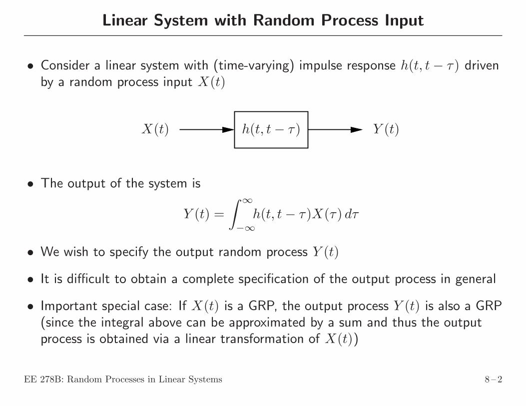
• Consider a linear system with (time-varying) impulse response h(t, t− τ) drivenby a random process input X(t)

PSfrag

X(t) Y (t)h(t, t− τ)

• The output of the system is

Y (t) =

∫ ∞

−∞

h(t, t− τ)X(τ) dτ

• We wish to specify the output random process Y (t)

• It is difficult to obtain a complete specification of the output process in general

• Important special case: If X(t) is a GRP, the output process Y (t) is also a GRP(since the integral above can be approximated by a sum and thus the outputprocess is obtained via a linear transformation of X(t))


• We focus on finding the mean and autocorrelation functions of Y (t) in terms ofthe mean and autocorrelation functions of the input process X(t) and theimpulse response of the system h(t, t− τ)

We are also interested in finding the crosscorrelation function between X(t) andY (t) defined as

RXY (t1, t2) = E(X(t1)Y (t2))

Note that unlike RX(t1, t2), RXY (t1, t2) is not necessarily symmetric in t1 andt2. However, RXY (t1, t2) = RY X(t2, t1)

• To find the mean of Y (t), consider

E(Y (t)) = E

(∫ ∞

−∞

h(t, t− τ)X(τ) dτ

)

=

∫ ∞

−∞

h(t, t− τ) E(X(τ)) dτ

• The crosscorrelation function between Y (t) and X(t) is

RY X(t1, t2) = E(Y (t1)X(t2))

= E

(∫ ∞

−∞

h(t1, t1 − τ)X(τ)X(t2) dτ

)

=

∫ ∞

−∞

h(t1, t1 − τ)RX(τ, t2) dτ


• The autocorrelation function of Y (t) is

RY (t1, t2) = E(Y (t1)Y (t2))

= E

(∫ ∞

−∞

h(t2, t2 − τ)X(τ)Y (t1) dτ

)

=

∫ ∞

−∞

h(t2, t2 − τ)RY X(t1, τ) dτ

=

∫ ∞

−∞

∫ ∞

−∞

h(t2, t2 − τ2)h(t1, t1 − τ1)RX(τ1, τ2) dτ1 dτ2

The average power isE(Y 2(t)) = RY (t, t)

• Example (Integrator): Let X(t) be a white noise process with autocorrelationfunction RX(τ) = (N/2)δ(τ) and let the linear system be an ideal integrator,i.e.,

Y (t) =

∫ t

0

X(τ) dτ

Find the mean and autocorrelation functions and the average power of theintegrator output Y (t), for t > 0


This example is motivated by several applications:

◦ Noise in an image sensor pixel: the white noise models the photodetector shotnoise, which is integrated with the signal over a capacitor before sampling

◦ Noise in a voltage controlled oscillator (for phase locked loops)

• Solution: The mean is

E(Y (t)) =

∫ t

0

E(X(τ)) dτ = 0

To obtain the autocorrelation function and average power for this case, we canspecialize the previous results to

RY X(t1, t2) =

∫ t1

0

N

2δ(t2 − τ) dτ

=

N

2, for t2 ≤ t1

0, otherwise


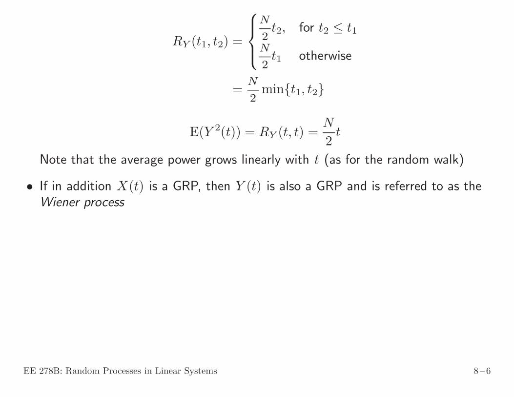
RY (t1, t2) =

N

2t2, for t2 ≤ t1

N

2t1 otherwise

=N

2min{t1, t2}

E(Y 2(t)) = RY (t, t) =N

2t

Note that the average power grows linearly with t (as for the random walk)

• If in addition X(t) is a GRP, then Y (t) is also a GRP and is referred to as theWiener process


LTI System with WSS Process Input

• Consider a linear time invariant (LTI) system with real impulse response h(t) andtransfer function H(f) = F(h(t)), driven by WSS process X(t), −∞ < t < ∞

PSfrag

X(t) Y (t)h(t)

• We want to characterize its output Y (t) = X(t) ∗ h(t) =∫ ∞

−∞

X(τ)h(t− τ)dτ

• It turns out (not surprisingly) that if the system is stable, i.e.,∣

∣

∣

∫∞

−∞h(t) dt

∣

∣

∣= |H(0)| < ∞, then X(t) and Y (t) are jointly WSS, which

means that:

◦ X(t) and Y (t) are WSS, and

◦ Their crosscorrelation function RXY (t1, t2) is time invariant, i.e.,

RXY (t1, t2) = E(X(t1)Y (t2)) = RXY (t1 + τ, t2 + τ) for all τ


• Relabel RXY (t1, t2) for jointly WSS X(t), Y (t) as RXY (τ), where τ = t1 − t2

RXY (τ) = RXY (t2 + τ, t2) = RXY (t2 + (t1 − t2), t2) = RXY (t1, t2)

Again RXY (τ) is not necessarily even. However,

RXY (τ) = RY X(−τ)

• Example: Let Θ ∼ U[0, 2π]. Consider two processes

X(t) = α cos(ωt+Θ) and Y (t) = α sin(ωt+Θ)

These processes are jointly WSS, since each is WSS (in fact SSS) and

RXY (t1, t2) = E[

α2 cos(ωt1 +Θ) sin(ωt2 +Θ)]

=α2

4π

∫ 2π

0

[

sin(ω(t1 + t2) + 2θ)− sin(ω(t1 − t2))]

dθ

= −α2

2sin(ω(t1 − t2))

• We define the cross power spectral density for jointly WSS processes X(t), Y (t)as

SXY (f) = F(RXY (τ))


• Example: Let Y (t) = X(t) + Z(t), where X(t) and Z(t) are zero meanuncorrelated WSS processes. Show that Y (t) and X(t) are jointly WSS, andfind RXY (τ) (in terms of RX and RZ) and SXY (f) (in terms of SX and SZ)

Solution: First, we show that Y (t) is WSS, since it is zero mean and

RY (t1, t2) = E[

(X(t1) + Z(t1))(X(t2) + Z(t2))]

= E(

X(t1)X(t2))

+ E(

Z(t1)Z(t2))

(X(t), Z(t) zero mean, uncorrelated)

= RX(τ) +RZ(τ)

Taking the Fourier transform of both sides, SY (f) = SX(f) + SZ(f)

To show that Y (t) and X(t) are jointly WSS, we need to show that theircrosscorrelation function is time invariant

RXY (t1, t2) = E[

X(t1)(X(t2) + Z(t2))]

= E(

X(t1)X(t2))

+ E(

X(t1)Z(t2))

= RX(t1, t2) + 0 (X(t), Z(t) zero mean, uncorrelated)

= RX(τ)

Taking the Fourier transform, SXY (f) = SX(f)


Output Mean, Autocorrelation, and PSD

Theorem: Let X(t), t ∈ R, be a WSS process input to a stable LTI system withreal impulse response h(t) and transfer function H(f). Then the input X(t) andoutput Y (t) are jointly WSS with:

1. E(Y (t)) = H(0) E(X(t))

2. RY X(τ) = h(τ) ∗RX(τ)

3. RY (τ) = h(τ) ∗RX(τ) ∗ h(−τ)

RX(τ) RY (τ)h(τ) h(−τ)RY X(τ)

4. SY X(f) = H(f)SX(f)

5. SY (f) = |H(f)|2SX(f)

SX(f) SY (f)H(f) H(−f)SY X(f)


Remark: For a discrete time WSS process X(n) and a stable LTI system h(n),X(n) and the output process Y (n) are jointly WSS and we can similarly findRY (n), . . .

Proof: Note that here the LTI system is in steady state

1. To find the mean of Y (t), consider

E(Y (t)) = E

(∫ ∞

−∞

X(τ)h(t− τ) dτ

)

=

∫ ∞

−∞

E(X(τ))h(t− τ) dτ

= E(X(t))

∫ ∞

−∞

h(t− τ) dτ = E(X(t))H(0)

2. To find the crosscorrelation function between Y (t) and X(t), consider

RY X(τ) = E(

Y (t+ τ)X(t))

= E

(∫ ∞

−∞

h(α)X(t+ τ − α)X(t) dα

)


=

∫ ∞

−∞

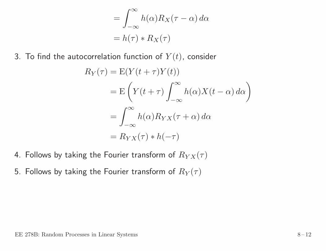
h(α)RX(τ − α) dα

= h(τ) ∗RX(τ)

3. To find the autocorrelation function of Y (t), consider

RY (τ) = E(Y (t+ τ)Y (t))

= E

(

Y (t+ τ)

∫ ∞

−∞

h(α)X(t− α) dα

)

=

∫ ∞

−∞

h(α)RY X(τ + α) dα

= RY X(τ) ∗ h(−τ)

4. Follows by taking the Fourier transform of RY X(τ)

5. Follows by taking the Fourier transform of RY (τ)


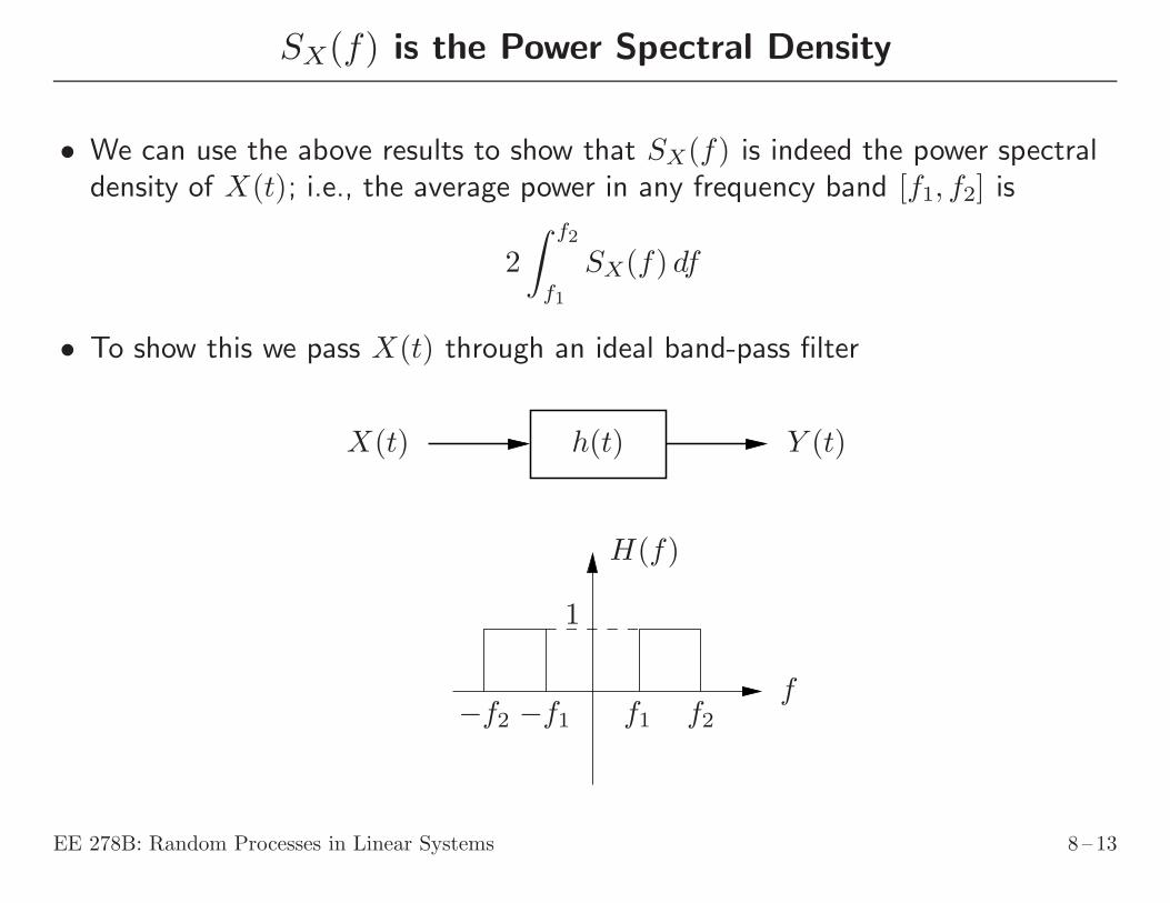
SX(f) is the Power Spectral Density

• We can use the above results to show that SX(f) is indeed the power spectraldensity of X(t); i.e., the average power in any frequency band [f1, f2] is

2

∫ f2

f1

SX(f) df

• To show this we pass X(t) through an ideal band-pass filter

X(t) Y (t)h(t)

H(f)

1

f−f2 −f1 f1 f2


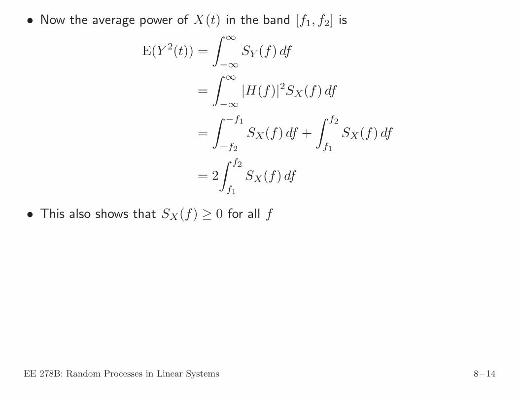
• Now the average power of X(t) in the band [f1, f2] is

E(Y 2(t)) =

∫ ∞

−∞

SY (f) df

=

∫ ∞

−∞

|H(f)|2SX(f) df

=

∫ −f1

−f2

SX(f) df +

∫ f2

f1

SX(f) df

= 2

∫ f2

f1

SX(f) df

• This also shows that SX(f) ≥ 0 for all f


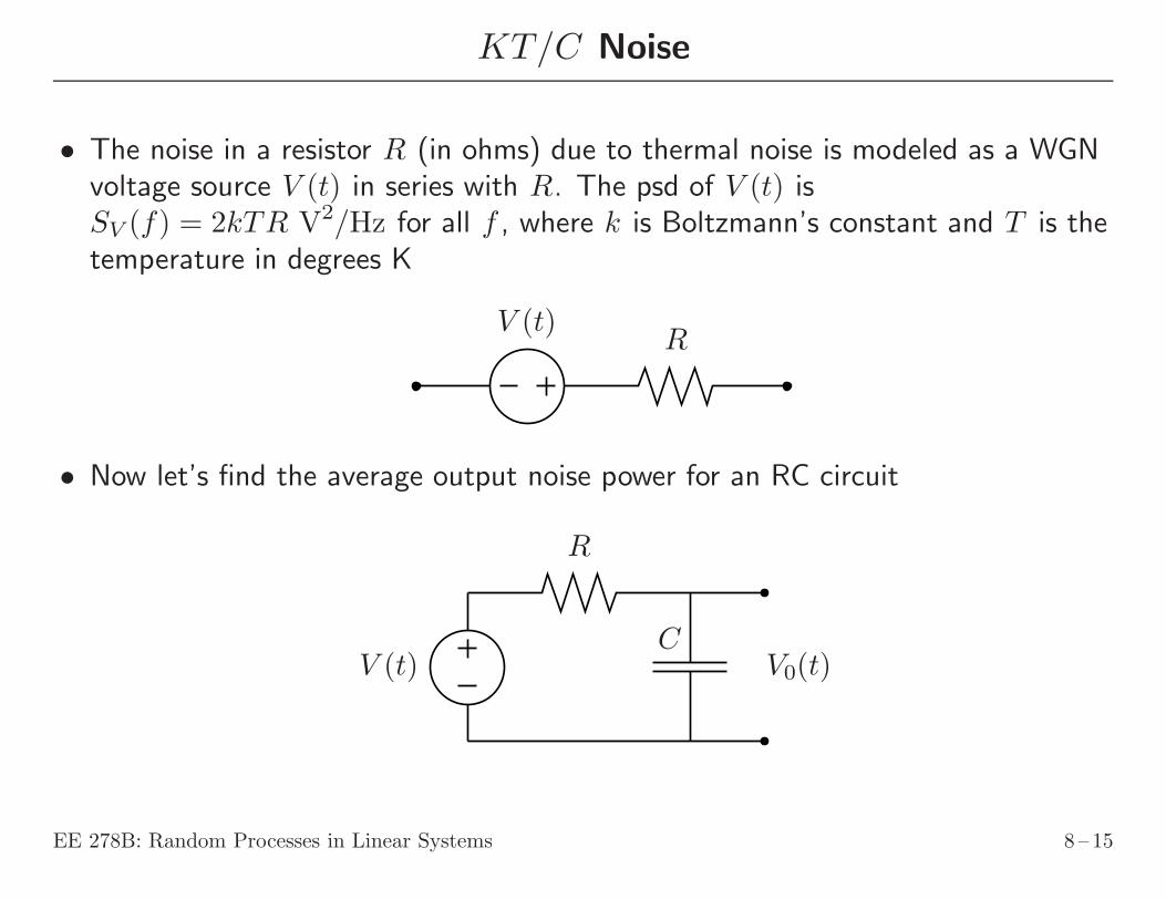
KT/C Noise

• The noise in a resistor R (in ohms) due to thermal noise is modeled as a WGNvoltage source V (t) in series with R. The psd of V (t) isSV (f) = 2kTR V2/Hz for all f , where k is Boltzmann’s constant and T is thetemperature in degrees K

V (t)R

• Now let’s find the average output noise power for an RC circuit

R

CV (t) V0(t)


• First we find the transfer function for the circuit

H(f) =1

1 + i2πfRC⇒ |H(f)|2 = 1

1 + (2πfRC)2

• Now we write the output psd in terms of the input psd as

SVo = SV (f)|H(f)|2 = 2kTR1

1 + (2πfRC)2, −∞ < f < ∞

• Thus the average output power is

E(V 2o (t)) =

∫ ∞

−∞

SVo(f)df

=2kTR

2πRC

∫ ∞

−∞

1

1 + (2πfRC)2d(2πfRC)

=kT

πC

∫ ∞

−∞

1

1 + x2dx

=kT

πCarctanx

∣

∣

∣

∣

+∞

−∞

=kT

πCπ =

kT

C,

which is independent of R!


Autoregressive Moving Average Process

• Let Xn, −∞ < n < ∞, be a discrete time white noise process with averagepower N

The autoregressive moving average (ARMA) process of order (p, q), Yn,−∞ < n < ∞, is defined as

Yn = −p

∑

k=1

αkYn−k +

q∑

l=0

βlXn−l

where β0 = 1, α1, . . . , αp and β1, . . . , βq are fixed parameters

• This process can be viewed as the output of an LTI system with transfer function

H(f) =1 +

∑ql=1 βle

−i2πfl

1 +∑p

k=1αke−i2πfk, |f | < 1

2

Therefore, the PSD of Yn is SY (f) = |H(f)|2N for |f | < 1/2


• Moving average (MA) process of order q: Let α1 = · · · = αp = 0, then Yn issimply a weighted sum of the q + 1 most recent Xn samples with weights(1, β1, . . . , βq), i.e.,

Yn =

q∑

l=0

βlXn−l, and the transfer function of the LTI system is

H(f) = 1 +

q∑

l=1

βle−i2πfl, |f | < 1

2

• Communication channel with intersymbol interference: The Xn processrepresents the transmitted information symbols and 1, β1, . . . , βq are thecoefficients of the channel impulse response

The process Yn is the interference-impaired received symbols

• Autoregressive (AR) process of order p: Let β1 = · · · = βn = 0. Then

Yn = −p

∑

k=1

αkYn−k +Xn, and the transfer function of the LTI system is

H(f) =1

1 +∑p

k=1αke−i2πfk, |f | < 1

2


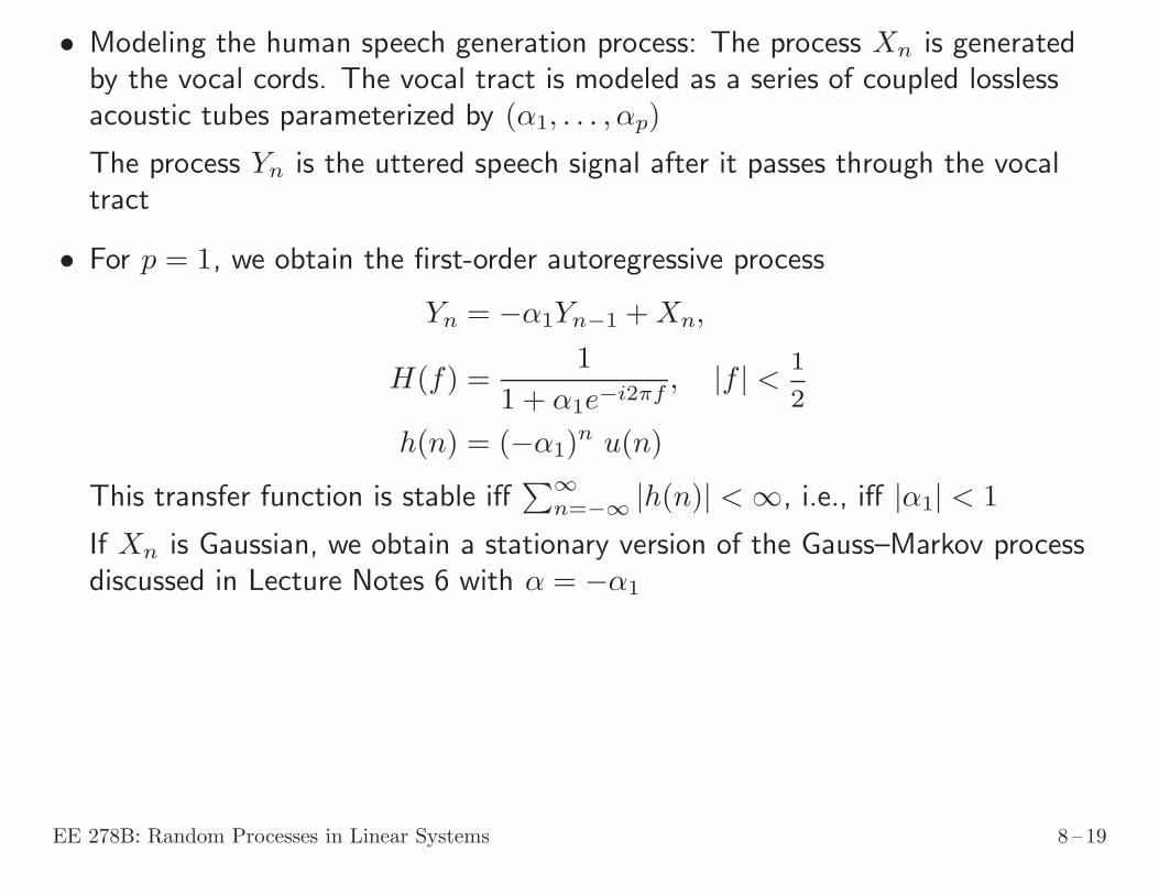
• Modeling the human speech generation process: The process Xn is generatedby the vocal cords. The vocal tract is modeled as a series of coupled losslessacoustic tubes parameterized by (α1, . . . , αp)

The process Yn is the uttered speech signal after it passes through the vocaltract

• For p = 1, we obtain the first-order autoregressive process

Yn = −α1Yn−1 +Xn,

H(f) =1

1 + α1e−i2πf, |f | < 1

2

h(n) = (−α1)n u(n)

This transfer function is stable iff∑∞

n=−∞ |h(n)| < ∞, i.e., iff |α1| < 1

If Xn is Gaussian, we obtain a stationary version of the Gauss–Markov processdiscussed in Lecture Notes 6 with α = −α1


Sampling Theorem for Bandlimited WSS Processes

• Recall the Nyquist sampling theorem for bandlimited deterministic signals:

◦ Let x(t) be a signal with Fourier transform X(f) such that X(f) = 0 forf /∈ [−B,B]

◦ We sample the signal at rate 1/T to obtain the sampled signal

yn = x(nT ) for n = . . . ,−2,−1, 0, 1, 2, . . .

The Fourier transform of the sequence yn,

Y (f) =∞∑

n=−∞

X(f − n/T ),

is periodic with period 1/T

◦ To recover the signal, we pass yn through an ideal low pass filter ofbandwidth 1/T . The Fourier transform of the reconstructed signal is

X(f) = Y (f) · ⊓(fT )

◦ Hence if the sampling rate 1/T ≥ 2B , X(f) = X(f) and the signal can bereconstructed perfectly from its samples


• It turns out that a similar result holds for sampling of bandlimited WSS randomprocesses

• Sampling theorem for WSS processes:

◦ Let X(t) be a continuous time WSS process with zero mean andautocorrelation function RX(τ) and PSD SX(f) = 0 for f /∈ [−B,B]

◦ We sample X(t) at rate 1/T to obtain the sampled (discrete time) processYn = X(nT ) with

µY (n) = E(Yn) = E(X(nT )) = 0,

RY (n1, n2) = E(Yn1Yn2) = E(X(n1T )X(n2T )) = RX((n1 − n2)T )

Hence Yn is WSS with zero mean and autocorrelation function

RY (n) = RX(nT )

The PSD of Yn,

SY (f) =∞∑

n=−∞

SX(f − n/T ),

is periodic with period 1/T


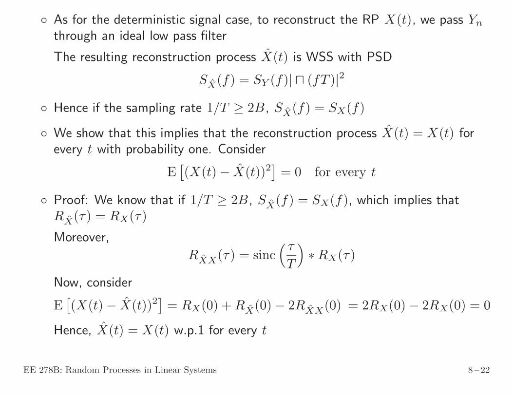
◦ As for the deterministic signal case, to reconstruct the RP X(t), we pass Yn

through an ideal low pass filter

The resulting reconstruction process X(t) is WSS with PSD

SX(f) = SY (f)| ⊓ (fT )|2

◦ Hence if the sampling rate 1/T ≥ 2B , SX(f) = SX(f)

◦ We show that this implies that the reconstruction process X(t) = X(t) forevery t with probability one. Consider

E[

(X(t)− X(t))2]

= 0 for every t

◦ Proof: We know that if 1/T ≥ 2B , SX(f) = SX(f), which implies thatRX(τ) = RX(τ)

Moreover,

RXX(τ) = sinc( τ

T

)

∗RX(τ)

Now, consider

E[

(X(t)− X(t))2]

= RX(0) +RX(0)− 2RXX(0) = 2RX(0)− 2RX(0) = 0

Hence, X(t) = X(t) w.p.1 for every t


Process Linear Estimation

• Let X(t) and Y (t) be zero mean jointly WSS processes with knownautocorrelation and crosscorrelation functions RX(τ), RY (τ), and RXY (τ)

• We observe the random process Y (α) for t− a ≤ α ≤ t+ b (−a ≤ b) and wishto find the MMSE linear estimate of the signal X(t), i.e., X(t) such that theMSE = E

[

(X(t)− X(t))2]

is minimized

• The linear estimate is of the form

X(t) =

∫ a

−b

h(τ)Y (t− τ) dτ

• By the orthogonality principle, the MMSE linear estimate must satisfy(

X(t)− X(t))

⊥ Y (t− τ) , −b ≤ τ ≤ a

orE[

(X(t)− X(t))Y (t− τ)]

= 0 , −b ≤ τ ≤ a


Thus, for −b ≤ τ ≤ a, we must have

RXY (τ) = E[

X(t)Y (t− τ)]

= E[

X(t)Y (t− τ)]

= E

(∫ a

−b

h(α)Y (t− α)Y (t− τ) dα

)

=

∫ a

−b

h(α)RY (τ − α) dα

So, to find h(α) we need to solve an infinite set of integral equations

• Solving these equations analytically is not possible in general. However, it canbe done for two important special cases:

◦ Infinite smoothing : when a, b → ∞◦ Filtering : when a → ∞ and b = 0 (Wiener–Hopf equations)


Infinite Smoothing Filter

• When a, b → ∞, the integral equations for the MMSE linear estimate become

RXY (τ) =

∫ ∞

−∞

h(α)RY (τ − α) dα , −∞ < τ < +∞

In other words,RXY (τ) = h(τ) ∗RY (τ)

• The Fourier transform convolution theorem gives the transfer function for theoptimal infinite smoothing filter :

SXY (f) = H(f)SY (f) ⇒ H(f) =SXY (f)

SY (f)


• The minimum MSE is

MSE = E[

(X(t)− X(t))2]

= E[

(X(t)− X(t))X(t)]

− E[

(X(t)− X(t))X(t)]

= E[

(X(t)− X(t))X(t)]

(by orthogonality)

= E[

(X(t)2]

− E[

X(t)X(t)]

To evaluate the second term, consider

RXX(τ) = E(X(t+ τ)X(t))

= E(

X(t+ τ)

∫ ∞

−∞

h(α)Y (t− α) dα)

=

∫ ∞

−∞

h(α)RXY (τ + α) dα = RXY (τ) ∗ h(−τ)

Therefore

E(X(t)X(t)) = RXX(0) =

∫ ∞

−∞

H(−f)SXY (f) df =

∫ ∞

−∞

|SXY (f)|2SY (f)

df ,


and the minimum MSE is

E[

(X(t)− X(t))2]

= E[

(X(t)2]

− E(

X(t)X(t))

=

∫ ∞

−∞

SX(f) df −∫ ∞

−∞

|SXY (f)|2SY (f)

df

=

∫ ∞

−∞

(

SX(f)− |SXY (f)|2SY (f)

)

df

• Example (Additive White Noise Channel): Let X(t) and Z(t) be zero meanuncorrelated WSS processes with

SX(f) =

{

P2 |f | ≤ B

0 otherwise

SZ(f) =N

2for all f

Here the signal X is bandlimited white noise, and Z is white noise

Find the optimal infinite smoothing filter for estimating X(t) given

Y (τ) = X(τ) + Z(τ) , −∞ < τ < +∞and the MSE for the estimate produced by this filter


The power spectral densities of X and Z are shown below

SX(f)

SZ(f)

H(f)

P2

N2

PP+N

f

f

f

−B

−B

B

B


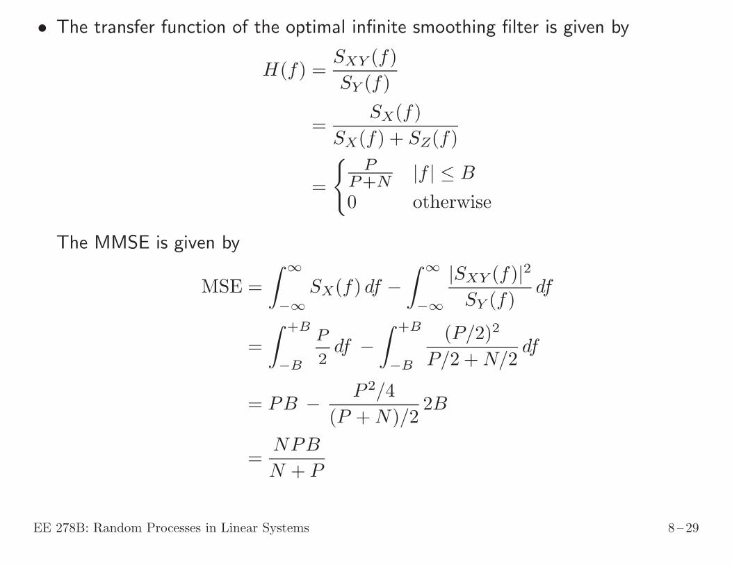
• The transfer function of the optimal infinite smoothing filter is given by

H(f) =SXY (f)

SY (f)

=SX(f)

SX(f) + SZ(f)

=

{

PP+N |f | ≤ B

0 otherwise

The MMSE is given by

MSE =

∫ ∞

−∞

SX(f) df −∫ ∞

−∞

|SXY (f)|2SY (f)

df

=

∫ +B

−B

P

2df −

∫ +B

−B

(P/2)2

P/2 +N/2df

= PB − P 2/4

(P +N)/22B

=NPB

N + P


Spectral Factorization

• It can be shown that the power spectral density SX(f) of WSS process X(t)has a square root, i.e., a transfer function H(f) such that

SX(f) = H(f)H∗(f) = |H(f)|2

This is similar to the square root of a covariance (correlation) matrix for arandom vector discussed in Lecture notes 4

• As for the random vector case, the square root of a PSD, H(f), and its inverse1/H(f) can be used for coloring and whitening of WSS processes, e.g.,

◦ Coloring:

X(t) H(f) Y (t)

SX(f) = 1 SY (f) = S(f)


◦ Whitening:

Y (t) 1/H(f) X(t)

SX(f) = 1SY (f) = S(f)

Here X(t) is the innovation process of Y (t)

• It turns out that under certain conditions, the PSD S(f) of a WSS process hasa causal square root, that is, S+(f) such that S(f) = S+(f)S−(f), whereS−(f) = (S+(f))∗ is an anticausal filter (note the similarity to the square rootfor correlation matrix via Cholesky decomposition)

• In particular, if S(f) is a rational PSD for a continuous time WSS process, i.e.,

S(f) = c(2πif + a1)(2πif + a2) . . . (2πif + am)

(2πif + b1)(2πif + b2) . . . (2πif + bn),

then it can be factorized into product of causal and anticausal square roots

Proof: Since S(f) is real and nonnegative, S∗(f) = S(f), if the denominatorhas factor (2πif + b), Re(b) > 0, then it must have factor (−2πif + b∗).Similarly, if numerator has factor (2πif + a), Re(a) > 0, then it must havefactor (−2πif + a∗)


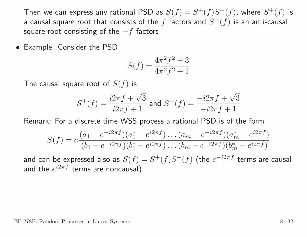
Then we can express any rational PSD as S(f) = S+(f)S−(f), where S+(f) isa causal square root that consists of the f factors and S−(f) is an anti-causalsquare root consisting of the −f factors

• Example: Consider the PSD

S(f) =4π2f2 + 3

4π2f2 + 1

The causal square root of S(f) is

S+(f) =i2πf +

√3

i2πf + 1and S−(f) =

−i2πf +√3

−i2πf + 1

Remark: For a discrete time WSS process a rational PSD is of the form

S(f) = c(a1 − e−i2πf)(a∗1 − ei2πf) . . . (am − e−i2πf)(a∗m − ei2πf)

(b1 − e−i2πf)(b∗1 − ei2πf) . . . (bm − e−i2πf)(b∗m − ei2πf)

and can be expressed also as S(f) = S+(f)S−(f) (the e−i2πf terms are causaland the ei2πf terms are noncausal)


• Example: Consider the PSD for a discrete time process

S(f) =3

5− 4 cos(2πf)

The causal square root is

S+(f) =

√3

2− e−i2πfand S−(f) =

√3

2− ei2πf

Spectral factorization theorem: In general, a PSD S(f) has a causal square rootif it satisfies the Paley-Wiener condition

∫ ∞

−∞

logS(f)

1 + 4π2fdf > −∞ for continuous time process

∫ 1/2

−1/2

logS(f) df > −∞ for discrete time process

• These condition are not always satisfied. For example they are not satisfied forbandlimited processes

• Remark: We assume throughout that F−1[S+(f)] is real ; henceS−(f) = S+(−f)


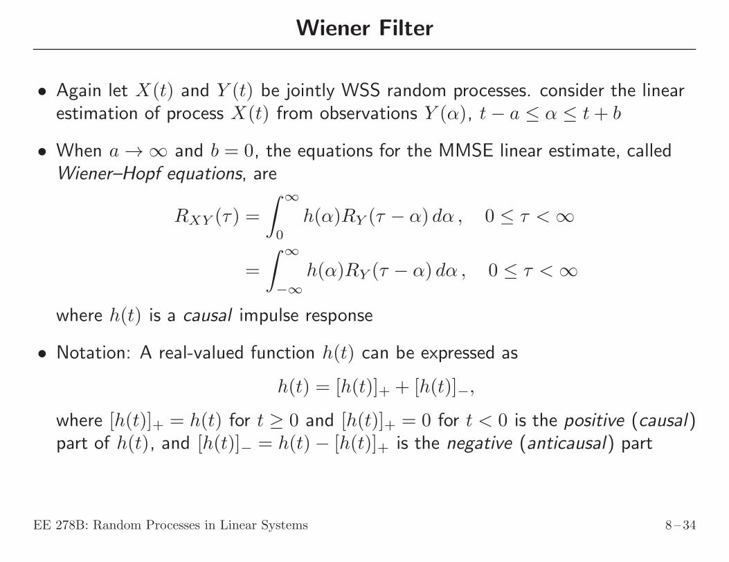
Wiener Filter

• Again let X(t) and Y (t) be jointly WSS random processes. consider the linearestimation of process X(t) from observations Y (α), t− a ≤ α ≤ t+ b

• When a → ∞ and b = 0, the equations for the MMSE linear estimate, calledWiener–Hopf equations, are

RXY (τ) =

∫ ∞

0

h(α)RY (τ − α) dα , 0 ≤ τ < ∞

=

∫ ∞

−∞

h(α)RY (τ − α) dα , 0 ≤ τ < ∞

where h(t) is a causal impulse response

• Notation: A real-valued function h(t) can be expressed as

h(t) = [h(t)]+ + [h(t)]−,

where [h(t)]+ = h(t) for t ≥ 0 and [h(t)]+ = 0 for t < 0 is the positive (causal)part of h(t), and [h(t)]− = h(t)− [h(t)]+ is the negative (anticausal) part


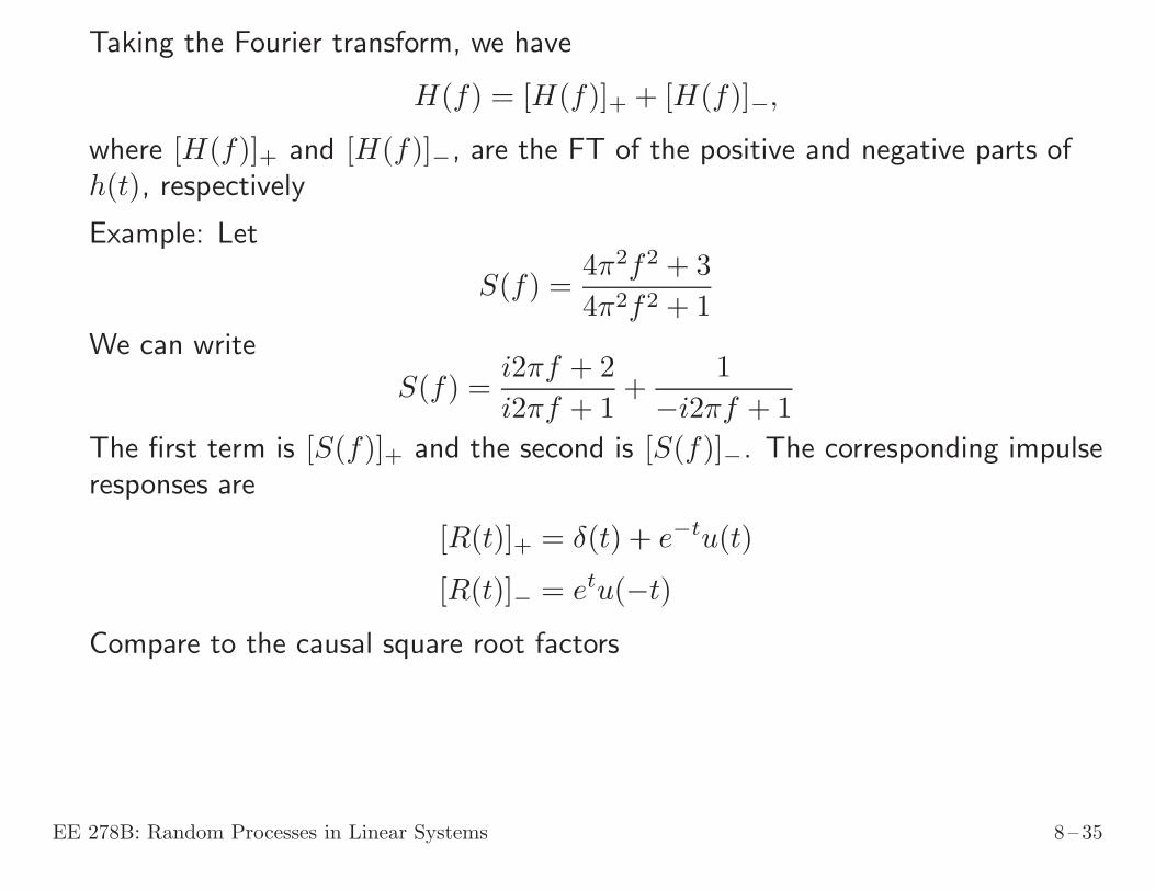
Taking the Fourier transform, we have

H(f) = [H(f)]+ + [H(f)]−,

where [H(f)]+ and [H(f)]−, are the FT of the positive and negative parts ofh(t), respectively

Example: Let

S(f) =4π2f2 + 3

4π2f2 + 1

We can write

S(f) =i2πf + 2

i2πf + 1+

1

−i2πf + 1

The first term is [S(f)]+ and the second is [S(f)]−. The corresponding impulseresponses are

[R(t)]+ = δ(t) + e−tu(t)

[R(t)]− = etu(−t)

Compare to the causal square root factors


• Now, back to the linear estimation problem. First assume that the observationprocess Y (τ) is white, i.e., RY (τ) = δ(τ), then the Wiener–Hopf equationsreduce to

RXY (τ) = h(τ) , 0 ≤ τ < ∞,

i.e., h(τ) = [RXY (τ)]+

and the corresponding transfer function is

H(f) =

∫ ∞

0

RXY (τ)e−2πifτ dτ,

i.e., H(f) = [SXY (f)]+

• For general SY (f) with causal square root S+Y (f), we first whiten the process to

obtain Y (τ) with RY (τ) = δ(τ), then convolve with [RXY (τ)]+

Y (t)1

S+Y(f) X(t)

Y (t)[SXY (f)]+


• Now to find RXY (τ), let g(t) = F−1[1/S+Y (f)] and consider

RXY (τ) = E(X(t+ τ)Y (τ))

= E(X(t+ τ)Y (t) ∗ g(t))= RXY (τ) ∗ g(−τ)

Taking the Fourier Transform we have

SXY (f) =SXY (f)

S−Y (f)

Hence,

[SXY (f)]+ =

[

SXY (f)

S−Y (f)

]

+

The transfer function of the Wiener filter is then given by

H(f) =1

S+Y (f)

[

SXY (f)

S−Y (f)

]

+


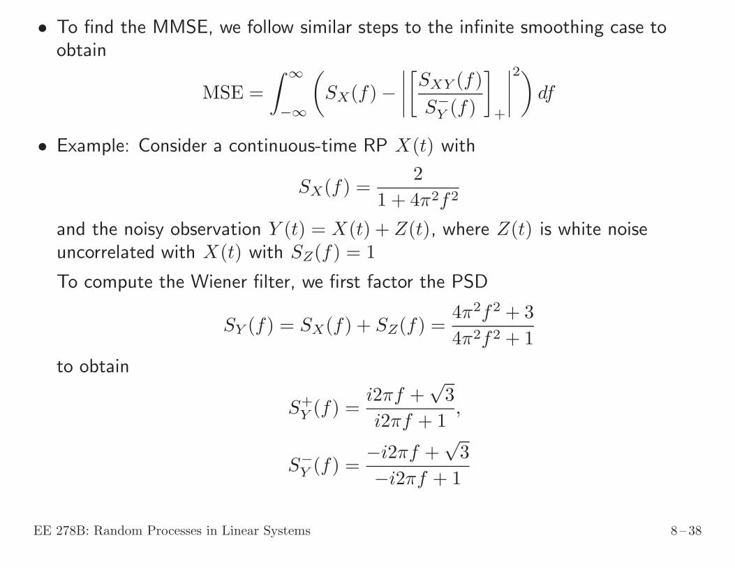
• To find the MMSE, we follow similar steps to the infinite smoothing case toobtain

MSE =

∫ ∞

−∞

(

SX(f)−∣

∣

∣

∣

[

SXY (f)

S−Y (f)

]

+

∣

∣

∣

∣

2)

df

• Example: Consider a continuous-time RP X(t) with

SX(f) =2

1 + 4π2f2

and the noisy observation Y (t) = X(t) + Z(t), where Z(t) is white noiseuncorrelated with X(t) with SZ(f) = 1

To compute the Wiener filter, we first factor the PSD

SY (f) = SX(f) + SZ(f) =4π2f2 + 3

4π2f2 + 1

to obtain

S+Y (f) =

i2πf +√3

i2πf + 1,

S−Y (f) =

−i2πf +√3

−i2πf + 1


The crosspower spectral density SXY (f) = SX(f), hence

SXY (f)

S−Y (f)

=2

1 + 4π2f2· −i2πf + 1

−i2πf +√3

=2

(i2πf + 1)(−i2πf +√3)

=

√3− 1

i2πf + 1+

√3− 1

−i2πf +√3

The first term is causal and the second term is anticausal. Therefore,[

SXY (f)

S−Y (f)

]

+

=

√3− 1

i2πf + 1

Hence, the Wiener filter is

H(f) =

√3− 1

i2πf +√3

h(t) = (√3− 1) e−

√3t u(t)


The MSE is

MSE =

∫ ∞

−∞

2√3− 2

1 + 4π2f2df =

√3− 1

• Example: Consider a discrete-time RP X(t) with

SX(f) =3

5− 4 cos(2πf)

and the noisy observation Y (t) = X(t) + Z(t), where Z(t) is white noise,independent of X(t), with SZ(f) = 1

Again we factor the PSD

SY (f) = SX(f) + SZ(f) =8− 4 cos(2πf)

5− 4 cos(2πf)

to obtain

S+Y (f) =

√

4− 2√3 · 2 +

√3− e−i2πf

2− e−i2πf

S−Y (f) =

√

4− 2√3 · 2 +

√3− ei2πf

2− ei2πf


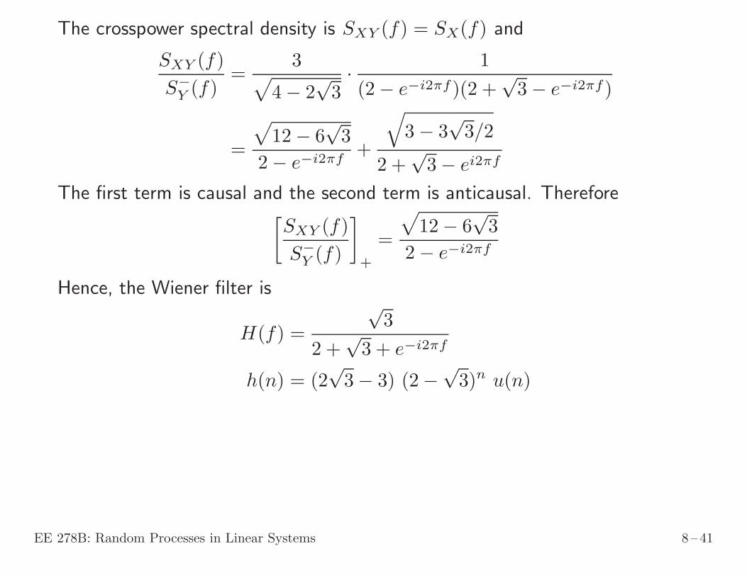
The crosspower spectral density is SXY (f) = SX(f) and

SXY (f)

S−Y (f)

=3

√

4− 2√3· 1

(2− e−i2πf)(2 +√3− e−i2πf)

=

√

12− 6√3

2− e−i2πf+

√

3− 3√3/2

2 +√3− ei2πf

The first term is causal and the second term is anticausal. Therefore[

SXY (f)

S−Y (f)

]

+

=

√

12− 6√3

2− e−i2πf

Hence, the Wiener filter is

H(f) =

√3

2 +√3 + e−i2πf

h(n) = (2√3− 3) (2−

√3)n u(n)


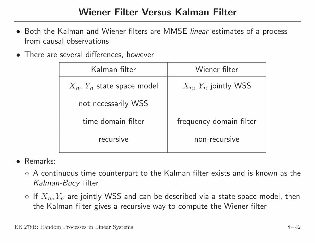
Wiener Filter Versus Kalman Filter

• Both the Kalman and Wiener filters are MMSE linear estimates of a processfrom causal observations

• There are several differences, however

Kalman filter Wiener filter

Xn, Yn state space model Xn, Yn jointly WSS

not necessarily WSS

time domain filter frequency domain filter

recursive non-recursive

• Remarks:

◦ A continuous time counterpart to the Kalman filter exists and is known as theKalman-Bucy filter

◦ If Xn, Yn are jointly WSS and can be described via a state space model, thenthe Kalman filter gives a recursive way to compute the Wiener filter


linear system with random process input lti system with … · · 2014-11-18• process linear...

Documents