computational elements for strapdown systems educational notes/rto-en... · computational elements...

Computational Elements for Strapdown Systems

Paul G. SavageStrapdown Associates, Inc.

Maple Plain, Minnesota 55359 USA

ABSTRACT

This paper provides an overview of the primary strapdown inertial system computational elements andtheir interrelationship. Using an aircraft type strapdown inertial navigation system as a representativeexample, the paper provides differential equations for attitude, velocity, position determination, associatedintegral solution functions, and representative algorithms for system computer implementation. For theinertial sensor errors, angular rate sensor and accelerometer analytical models are presented includingassociated compensation algorithms for correction in the system computer. Sensor compensationtechniques are discussed for coning, sculling, scrolling computation algorithms and for accelerometer outputadjustment for physical size effect separation and anisoinertia error. Navigation error parameters aredescribed and related to errors in the system computed attitude, velocity, position solutions. Differentialequations for the navigation error parameters are presented showing error parameter propagation in responseto residual inertial sensor errors (following sensor compensation) and to errors in the gravity model used inthe system computer.

COORDINATE FRAMES

As used in this paper, a coordinate frame is an analytical abstraction defined by three mutuallyperpendicular unit vectors. A coordinate frame can be visualized as a set of three perpendicular lines (axes)passing through a common point (origin) with the unit vectors emanating from the origin along the axes. Inthis paper, the physical position of each coordinate frame’s origin is arbitrary. The principal coordinateframes utilized are the following:

B Frame = "Body" coordinate frame parallel to strapdown inertial sensor axes.N Frame = "Navigation" coordinate frame having Z axis parallel to the upward vertical at the local

position location. A "wander azimuth" N Frame has the horizontal X, Y axes rotatingrelative to non-rotating inertial space at the local vertical component of earth's rateabout the Z axis. A "free azimuth" N Frame would have zero inertial rotation rate ofthe X, Y axes around the Z axis. A "geographic" N Frame would have the X, Y axesrotated around Z to maintain the Y axis parallel to local true north.

E Frame = "Earth" referenced coordinate frame with fixed angular geometry relative to the rotatingearth.

I Frame = "Inertial" non-rotating coordinate frame.

NOTATION

V = Vector without specific coordinate frame designation. A vector is a parameter that has lengthand direction. Vectors used in the paper are classified as “free vectors”, hence, have nopreferred location in coordinate frames in which they are analytically described.

VA = Column matrix with elements equal to the projection of V on Coordinate Frame A axes. Theprojection of V on each Frame A axis equals the dot product of V with the coordinate FrameA axis unit vector.

RTO-EN-SET-116(2008) 3 - 1

VA × = Skew symmetric (or cross-product) form of VA represented by the square matrix0 - VZA VYA

VZA 0 - VXA

- VYA VXA 0

in which VXA , VYA , VZA are the components of VA. The

matrix product of VA × with another A Frame vector equals the cross-product of VA

with the vector in the A Frame.

CA2

A1 = Direction cosine matrix that transforms a vector from its Coordinate Frame A2 projection

form to its Coordinate Frame A1 projection form.

ωA1A2 = Angular rate of Coordinate Frame A2 relative to Coordinate Frame A1. When A1 is non-

rotating, ωA1A2 is the angular rate that would be measured by angular rate sensors

mounted on Frame A2.

= d dt

= Derivative with respect to time.

t = Time.

1. INTRODUCTION

The primary computational elements in a strapdown inertial navigation system (INS) consist ofintegration operations for calculating attitude, velocity and position navigation parameters using strapdownangular rate and specific force acceleration for input. The computational form of these operations originatefrom two basic sources: time rate differential equations for the navigation parameters and analytical errormodels describing the error characteristics of the strapdown inertial angular rate sensors and accelerometersproviding the angular rate and specific force acceleration measurement data. The latter is the source forcompensation algorithms used in the system computer to correct predictable errors in the inertial sensoroutputs. The former is the source for digital integration algorithms resident in system software forcomputing the navigation parameters. Both are the source for error propagation equations used to describethe behavior of navigation parameter errors in the presence of residual sensor errors remaining aftercompensation.

This paper provides examples of each of the aforementioned computational elements and theirinterrelationship. For the digital integration algorithms, the examples are selected to emphasize a structuralgoal of being based (to the greatest extent possible) on closed-form analytically exact integral solutions tothe navigation parameter time rate differential equations. Such a structure significantly simplifies theintegration algorithm software validation process based on a comparison with closed-form exact solutiondynamic model simulators designed to thoroughly exercise the exact solution algorithms under test(Reference 26). For properly derived and programmed algorithms, the comparison will yield identicallyzero difference, thereby providing a clear unambiguous algorithm software validation. Once validated, suchalgorithms can be used as a generic set suitable for all strapdown inertial applications. Associated algorithmdocumentation is also simplified because algorithm derivations are classical analytical formulations andexplanations/numerical-error-analysis justification for application dependent approximations are notrequired because there are none. Modern day strapdown system computer technology (high throughput,long floating point word-length) allows the general use of such exact solution algorithms without penalty.Similarly, the sensor compensation algorithms shown in the paper are a generic set based on the exactinverse of classical sensor error models without first order approximations (as has been commonly used inthe past to save on computer throughput).

The form of the navigation error propagation equations are based on analytical definitions of the attitude,velocity, position error parameters. Several choices are possible. Two of the most common sets are


3 - 2 RTO-EN-SET-116(2008)

illustrated in the paper and equivalencies between the two described. An example of the error propagationequations based on one of the sets is provided.

This paper is an updated version of Reference 22. Reference 22 is a condensed summary of materialoriginally published in the two volume textbook Strapdown Analytics (Ref. 20), the second edition of whichhas been recently published (Reference 25). Strapdown Analytics provides a broad detailed exposition ofthe analytical aspects of strapdown inertial navigation technology. This version of the Reference 22 paperalso incorporates new material from the recently published paper A Unified Mathematical Framework ForStrapdown Algorithm Design (Reference 23) - also provided in Section 19.1 of the second edition ofStrapdown Analytics (Reference 25). Equations in this paper (as in Reference 22) are presented withoutproof. Their derivations are provided in Reference 20 (or 25) and in Reference 23 as delineated throughoutthe paper (by Reference 20 or 25 section number and by Reference 23 equation number). Documentsdelineated in the paper's References listing that are not cited in the body of the paper are those cited inReference 20 (or 25) that are specifically related to the paper's subject matter.

2. REPRESENTATIVE STRAPDOWN INERTIAL NAVIGATION DIFFERENTIALEQUATIONS

This section describes a typical set of basic attitude/velocity/position integration and accelerationtransformation operations performed in a strapdown INS. The integration operations are described in theform of continuous differential equations that when integrated in the classical analytical continuous sense,provide the attitude, velocity and position data generated digitally in the strapdown system computer. Thealgorithms described in Section 4 are designed to achieve the same numerical result by digital integration asthe continuous integration of the differential equations presented in this section.

2.1 Attitude

For a terrestrial (earth) based inertial navigation system (e.g., for aircraft), sensor assembly angularattitude orientation is usually described as an “attitude direction cosine matrix” (or attitude quaternion)relating sensor assembly axes (the “body” or B Frame) to locally level attitude reference coordinates (NFrame). Attitude determination consists of integrating the associated time rate differential equations for theselected attitude parameters. For an attitude reference formulation based on direction cosines the attitudetime rate differential equations are given by (Ref. 20 (or 25) Sects. 4.1 and 4.1.1):

CBN

= CBN

ωIBB

× - ωINN

× CBN

ωIEN

= CNE T

ωIE E

ωENN

≡ ρN = FC

N uUp

N × vN + ρZN uZN

N (1)

ωINN

= ωIEN

+ ωENN

where

ρN = Conventional notation for ωEN

N, also known as “transport rate”, and analytically defined as

the angular rate of Frame N relative to Frame E.

ρZN = Vertical component of ρN. For a "wander azimuth" N Frame, ρZN is zero. For a "free

azimuth" N Frame, ρZN is the downward vertical component of earth's inertial angular rate.

FCN

= Curvature matrix in the N Frame that is a function of position location over the earth.

v = Velocity (rate of change of position) relative to the earth.uUp = Unit vector upward at the current position location (parallel to the N Frame Z axis).


RTO-EN-SET-116(2008) 3 - 3

The equivalent quaternion formulation (Ref. 20 (or 25) Sect. 4.1) is as follows:

qBN

= 12

qBN

ωIBB

- 12

ωINN

qBN

(2)

where

qBN

= Attitude quaternion relating coordinate Frames B and N.

ωIBB

, ωINN

= Quaternions with vector components equal to ωIBB

, ωINN

and zero for the scalar

components.

The CNE

matrix in Equations (1) defines the system angular position location in earth reference

coordinates, hence, is sometimes denoted as the “position” direction cosine matrix (or the equivalent

position quaternion). The CNE

matrix is calculated by integrating its differential equation (described in

Section 2.3) using ωINN

(N Frame "platform" rotation rate) as input. For earth's zero altitude surface

reference modeled as an ellipsoid of revolution around earth's rotation axis (i.e., the conventional approach),

Reference 20 (or 25) Sections 5.2.4 and 5.3 develop the following exact expression for the FCN

curvature

matrix in Equations (1) based on an E Frame definition having Y axis parallel to earth's axis of rotation:

FCN

=

FC11 FC12 0

FC21 FC22 0

0 0 0

FC11 = 1rl

1 + D212

feh FC12 = 1rl

D21 D22 feh

FC21 = 1rl

D21 D22 feh FC22 = 1rl

1 + D222

feh (3)

rl = R0 (1 - e) 2

1 + D232

1 - e 2 - 1 3 / 2

+ h

feh ≡ 1 - e 2 - 1

1 + D232

1 - e 2 - 1 1 + h

R0 1 + D23

2 1 - e 2 - 1

where

Dij = Element in row i column j of CNE

.

e = Ellipticity of earth's reference surface ellipsoid.R0 = Earth's equatorial radius.rl = Local radius of curvature at altitude in the North/South (latitude change) direction.h = Altitude from earth's reference surface ellipsoid to the current position location (positive above

the earth's surface).

2.2 Velocity

The velocity data in an inertial navigation system is typically computed as an integration of velocity ratedescribed in the navigation N Frame. The velocity of interest is usually defined as the time rate of changeof position relative to the earth in a coordinate frame that rotates at earth's rotation rates (i.e., the E Frame):


3 - 4 RTO-EN-SET-116(2008)

vE ≡ RE

(4)

whereR = Position vector from earth's center to the current position location.

In the N Frame, the velocity is then:

vN = CEN

vE (5)

Based on this definition, the time rate differential equation for velocity is (Ref. 20 (or 25) Sect. 4.3):

vN

= CBN

aSFB

+ gN - ωIEN

× ωIE N

× RN - ωINN

+ ωIEN

× vN (6)

whereaSF = Specific force acceleration defined as the instantaneous time rate of change of velocity

imparted to a body relative to the velocity it would have sustained without disturbances inlocal gravitational vacuum space. Sometimes defined as total velocity change rate minusgravity. Accelerometers measure aSF .

g = Mass attraction gravity at the current position location minus mass attraction gravity at the

center of the earth. Sometimes denoted as "gravitation" (Ref. 2 Sect. 4.4).

For the quaternion attitude formulation approach in Section 2.1, the CBN

aSFB

term in Equation (6) would

be replaced by the vector part of the quaternion product qBN

aSFB

qBN

* in which qBN

* is the conjugate of qBN

and aSFB

is the quaternion with aSFB

for its vector component and zero for its scalar component.

Alternatively, once qBN

is calculated by integrating Equation (2), it can be converted to the equivalent CBN

direction cosine matrix (Ref. 20 (or 25) Sect. 7.1.2.4) which is then directly compatible with Equation (6) asshown.

Reference 20 (or 25) Section 5.4.1 shows how gN - ωIEN

× ωIE N

× RN in Equation (6) can be calculated

without singularities based on a classical gravity model defined in the E Frame (Ref. 2 Sect. 4.4 and Ref. 3).The latter references model gravity on and above earth's zero altitude surface. Reference 20 (25) Section5.4 extends the model for negative altitudes (i.e., below earth's surface).

2.3 Position

Position relative to the earth is often described by altitude above the earth and the angular orientation ofthe current local vertical direction in earth coordinates (the E Frame). The angular position parameters arecommonly represented by latitude and longitude, however, to avoid mathematical singularities, the angularposition parameters are frequently represented in the form of the N to E position direction cosine matrix (orthe equivalent quaternion). The time rate differential equations for the position direction cosine matrix andaltitude are as follows (Ref. 20 (or 25) Sects. 4.4.1.1 and 4.4.1.2):

CNE

= CNE

ρN× h = uUpN

⋅ vN (7)

2.4 Attitude, Velocity, Position Output Conversion

An advantage for using CBN

, CNE

(or their quaternion equivalents), vN, and h as the basic navigation

parameters calculated by integration is that the associated differential equations have no singularities for all


RTO-EN-SET-116(2008) 3 - 5

INS attitude orientations and position locations. Once calculated, they can be output from the INS directlyand/or converted into other formats for output (e.g., roll, pitch, heading attitude; north, east, verticalvelocity; latitude, longitude, altitude position - Ref. 20 (or 25) Sects. 4.1.2, 4.3.1, and 4.4.2.1).

3. Integral Solutions For The Navigation Parameters

The digital integration algorithms resident in the strapdown system computer are based on integratedforms of the Section 2 navigation parameter differential equations over a digital integration update cycle.For modern day algorithms, the integrated form is structured into two operations; 1. Basic digital updatingoperations used to increment the attitude/velocity/position parameters over each update cycle, and 2. Highspeed integration operations that account for high frequency angular-rate/acceleration inputs between eachupdate cycle (coning effects in attitude determination, sculling effects in velocity determination, andscrolling effects in position determination). The bulk of the computations are contained in the basicoperations that can be structured based on closed-form exact integral solutions to the Section 2 differentialequations. Use of exact closed-form solutions for the basic operations translates directly into computerintegration algorithm forms that are easily verified by simple and direct simulation techniques (Ref. 26).

3.1 Attitude

The classical exact integral solution to the Section 2.1 direction cosine attitude rate equation is as follows(Ref. 20 (or 25) Sects. 7.1.1, 7.1.1.1, and 7.1.1.2):

CBm

Nm-1 = CBm-1

Nm-1 CBI(m)

BI(m-1)

CBm

Nm = CNI(m-1)

NI(m) CBm

Nm-1

CBI(m)

BI(m-1) = I + f1(φm) φm× + f2(φm) φm× 2

(8)

CNI(m-1)

NI(m) = I - f1(ζm) ζm× + f2(ζm) ζm× 2

f1 (χ) ≡ sin χ

χ f2 (χ) ≡

1 - cos χ

χ2

wherem = System computer cycle time index for basic navigation parameter updating.Bm, Nm = Coordinate Frame B and N orientations at navigation computer cycle time m.BI(m) , NI(m) = Discrete orientation of the B and N Frames in non-rotating inertial space (I) at

computer cycle time tm.I = Identity matrix.

φm, ζm = Rotation vector equivalents to the CBI(m)

BI(m-1) and CNI(m-1)

NI(m) direction cosine matrices (See

Reference 20 (or 25) Section 3.2.2 for rotation vector definition).

φm, ζm = Magnitudes of φm, ζm.

χ = Dummy angle parameter.

Reference 20 (or 25) Sections 7.1.2, 7.1.2.1 and 7.1.2.2 provide the equivalent quaternion formulation

integral solution which also is a function of the identical φm, ζm rotation vectors.


3 - 6 RTO-EN-SET-116(2008)

Under constant inertial angular rates of the B and N Frames (ωIBB

and ωINN

), the φm, ζm rotation vectors

equal the simple integral of the B and N Frame inertial angular rates over the tm-1 to tm time interval.

Under dynamic angular rate conditions, φm, ζm contain small additional "coning" terms that account for

dynamic variations. The computation of φm and ζm is discussed in Section 3.4.

All of Equations (8) are analytically exact under general dynamic angular-rate conditions. An importantpoint to recognize is that both direction cosine and quaternion based attitude algorithms have exact solutions

using the identical φm, ζm rotation vector inputs. Hence, contrary to outdated popular belief, modern dayquaternion and direction cosine attitude algorithm formulations have equal accuracy.

3.2 Velocity

The velocity algorithm implemented in the navigation software can be formulated from the integral ofEquation (6) using a trapezoidal integration approximation for the small and/or slowly varying terms (Ref.20 (or 25) Sects. 7.2, 7.2.2, 7.2.2.2 and 7.2.2.2.1 - note correction to Equation (7.2.2-4)):

vmN

= vm-1N

+ ΔvSFm

N + ΔvG/CORm

N

ΔvG/CORm

N = vG/COR

N dt

tm-1

tm

≈ 12

3 vG/CORm-1

N - vG/CORm-2

N Tm

vG/CORN

≡ gN - ωIEN

× ωIE N

× RN - ωINN

+ ωIEN

× vN

ΔvSFm

N =

12

CNI(m-1)

NI(m) + I ΔvSFm

Nm-1 ≈

12

2 CNI(m-2)

NI(m-1) - CNI(m-3)

NI(m-2) + I ΔvSFm

Nm-1(9)

ΔvSFm

Nm-1 = CBm-1

Nm-1 ΔvSFm

Bm-1

ΔvSFm

Bm-1 = CBI (t)

BI(m-1) aSFB

dttm-1

tm

= I + f2(φm) φm× + f3(φm) φm× 2

ηm

CBI (t)BI(m-1) = I + CBI (t)

BI(m-1) ωIBB

× dτtm-1

t

f3 (χ) ≡ 1

χ2 1 -

sin χ

χ

whereBI(t) = B Frame orientation in non-rotating inertial space at time t after tm-1.

ΔvSFm = Velocity change from computer cycle m-1 to m due to specific force acceleration.

ΔvG/CORm = Velocity change from computer cycle m-1 to m due to gravity and Coriolis

acceleration. The approximate form shown is an extrapolation based on past (not yetupdated) values of velocity and position.

ηm = Velocity translation vector from computer cycle m-1 to m.t = General time in navigation.

τ = Dummy time parameter.


RTO-EN-SET-116(2008) 3 - 7

The approximate form shown for ΔvSFm

N is based on CNI(m-1)

NI(m) (part of the Equations (8) with (18) attitude

computations) being updated following the velocity and position update.

The ΔvSFm

Bm-1 expression in Equations (9) utilizes a velocity translation vector ηm (analogous to the rotation

vector φm) to generate an analytically exact solution for ΔvSFm

Bm-1 under general dynamic angular-

rate/specific-force conditions. The velocity translation vector concept was introduced by the author inReference 23 as part of a unified framework for strapdown attitude/velocity/position integration algorithm

formulation. Under constant B Frame specific force and inertial angular rate (aSFB

and ωIBB

), the ηm velocity

translation vector equals the simple integral of B Frame specific force over the tm-1 to tm time interval.

Under dynamic angular-rate/specific-force conditions, ηm contains a small additional "sculling" term that

accounts for dynamic variations. The computation of ηm is discussed in Section 3.4.

Except for trapezoidal integration error in the small and/or slowly varying terms, all of Equations (9) areanalytically exact under general dynamic angular-rate/specific-force conditions.

3.3 Position

The position algorithm implemented in the navigation software can be formulated from the integral ofEquations (7) using an extrapolated trapezoidal integration approximation for the small and/or slowlyvarying terms (Ref. 20 (or 25) Sects. 7.3.1, 7.3.3 and 7.3.3.1 - note correction to Equations (7.3.3-4)):

hm = hm-1 + Δhm

CNE(m)

E = CNE(m-1)

E CNE(m)

NE(m-1)

CNE(m)

NE(m-1) = I + f1 ξm + f2 ξm ξm× ξm×

ξm ≈ ρN dt

tm-1

tm

≈ 12

3 ρZNm-1 - ρZNm-2 uUpN

Tm + 3 FCm-1

N - FCm-2

N uUp

N × ΔRm

N

Δhm = uUpN

⋅ ΔRmN

ΔRmN

≡ vN dttm-1

tm

≈ vm-1N

+ 12

ΔvG/CORm

N Tm + ΔRSFm

N(10)

ΔRSFm

N =

16

CNm-1

Nm - I ΔvSFm

Nm-1 Tm + CBm-1

Nm-1 ΔRSFm

Bm-1

≈ 16

2 CNm-2

Nm-1 - CNm-3

Nm-2 - I ΔvSFm

Nm-1 Tm + CBm-1

Nm-1 ΔRSFm

Bm-1

ΔRSFm

Bm-1 = tm-1

t

CBI(τ1)BI(m-1) aSF

B dτ1 dτ

tm-1

τ

= I + 2 f3(φm) φm × + 2 f4(φm) φm × 2 κm

f4 (χ) ≡ 1

χ2

12

- 1 - cos χ

χ2


3 - 8 RTO-EN-SET-116(2008)

whereNE(m) = Discrete orientation of the N Frame in rotating earth space (E) at computer cycle time tm.

ξm = Rotation vector equivalent to the CNE(m)

NE(m-1) direction cosine matrix. The computation is an

extrapolated trapezoidal approximation to the exact integral of ξ over an m cycle (similar to

the Section 3.4 Equation (18) approximation for the integral of ζ in Equation (11), but using

ρN in place of ωIN

N).

ξm = Magnitude of ξm.

ζm = Calculated in Section 3.4 Equations (18).

Δhm = Altitude change from computer cycle m-1 to m.

ΔRm = Position vector change from computer cycle m-1 to m.

ΔRSFm = Specific force acceleration contribution to ΔRm.

κm = Position translation vector from cycle m-1 to m.

The ΔRSFm

Bm-1 expression in Equations (10) utilizes a position translation vector κm (analogous to the

rotation vector φm) to generate an analytically exact solution for ΔRSFm

Bm-1 under general dynamic angular-

rate/specific-force conditions. The position translation vector concept was introduced by the author inReference 23 as part of a unified framework for strapdown attitude/velocity/position integration algorithm

formulation. Under constant B Frame specific force and inertial angular rate (aSFB

and ωIBB

), the κm position

translation vector equals the simple double integral of B Frame specific force over the tm-1 to tm time

interval. Under dynamic angular-rate/specific-force conditions, κm contains a small additional "scrolling"

term that accounts for dynamic variations. The computation of κm is discussed in Section 3.4.

Except for trapezoidal integration error in the small and/or slowly varying terms, all of Equations (10) areanalytically exact under general dynamic angular-rate/specific-force conditions.

3.4 Computing The Rotation And Translation Vectors

The form of the CBI(m)

BI(m-1), CNI(m-1)

NI(m) expressions in (8) can be derived as the exact solution to Equations (1)

under constant B and N Frame inertial angular rate (Ref. 20 (or 25) Sects. 3.2.2 and 3.2.2.1). The resultwould be identical to (8), but with the rotation vectors replaced by the integrals of the B and N Frame

inertial rotation rates. Similarly, the forms of the ΔvSFm

Bm-1and ΔRSFm

Bm-1 expressions in (9) and (10) can be

derived as the exact analytic solution to the integrals in these expressions under constant B Frame inertialangular rate and specific force (Refs. 19 and 20 (or 25) Sects. 7.2.2.2 and 7.3.3). The result would be

identical to the ΔvSFm

Bm-1 and ΔRSFm

Bm-1 expressions in (9) and (10), but with the rotation vector replaced by

integrated B Frame angular rate and the velocity/position translation vectors replaced by the integral and

double integral of B Frame specific force. In fact, the ΔvSFm

Bm-1 and ΔRSFm

Bm-1 expressions in (9) and (10) were

derived in Reference 23 as the aforementioned exact solution under constant B Frame angular-rate/specific-force solution, but for general motion having the integrated B Frame angular rate term replaced by therotation vector and the integrated/doubly-integrated B Frame specific force terms replaced by the translation

vectors. This is the same approach used by Jordan in Reference 8 for introducing the CBI(m)

BI(m-1) expression in


RTO-EN-SET-116(2008) 3 - 9

(8) (which has been extended in this paper to also include CNI(m-1)

NI(m) ). For the Jordan case, the rotation vector

was formulated by approximation as integrated angular rate plus a coning correction based on theGoodman-Robinson theorem (Ref. 4). The rotation vector concept was introduced by Euler and utilized byLaning in 1949 (Ref. 10) to develop the classical exact rotation vector rate of change equation (shownsubsequently in this section) for strapdown inertial navigation application. Note: In 1971 Bortzreintroduced and applied the exact Laning rotation vector rate equation in a strapdown system/softwareimplementation (Ref. 1) for which it has since been known as the "Bortz equation".

The integral of the Laning rotation vector rate equation provides an exact solution for the rotation vector

input to the CBI(m)

BI(m-1), CNI(m-1)

NI(m) expressions in (8). Based on the previous discussion, the velocity/ position

translation vectors ηm, κm can be analytically defined as the vectors that satisfy the ΔvSFm

Bm-1 expression in

(9) and the ΔRSFm

Bm-1 expression in (10). Using this definition, References 23 or 25 (Section 19.1.5) derive

analytically exact equations for the translation vector rates of change (shown subsequently) which, when

integrated from time tm-1 to tm, provide exact solutions for ηm and κm. References 23, 25 Sect. 19.1, and20 (or 25) Sect. 7.1.1.2 then show that the following simplified forms can be utilized as accurate

approximations for the φ, ζ, η and κ rotation/translation vector rates (Ref. 23 Equations (31) or Ref. 25

Equations (19.1.8-3), and Ref. 20 (or 25) Equation (7.1.1.2-4)):

φ ≈ ωIBB +

12

α(t) × ωIBB α(t) ≡ ωIB

B dτ

tm-1

t

ζ ≈ ωINN

η ≈ aSFB

+ 12

α(t) × aSFB

- ωIBB

× υ(t) υ(t) ≡ aSFB

dτtm-1

t

(11)

κ = η(t) + 16

α(t) × υ(t) - 2 ωIBB

× Sυ(t) Sυ(t) ≡ υ dτtm-1

t

The error in the Equations (11) approximation is minimized by using a small value for the computer

update cycle time interval tm-1 to tm, thereby assuring small values of φ and ζ. Using Equations (1) for ωINN

with a trapezoidal integration algorithm (Ref. 20 (or 25) Sect. 7.1.1.2.1), the integral of Equations (11) overa computer update cycle then becomes for the rotation/translation vector inputs to Equations (8), (9) and(10):

φm = αm + Δ φConem ηm = υm + ΔηSculm κm = Sυm + ΔκScrlm (12)

ΔφConem = 12

α t × ωIBB

dttm-1

tm

Coning (13)

ΔηScul (t) = 12

α(τ) × aSFB

+ υ(τ) × ωIBB

dτtm-1

t

ΔηSculm = ΔηScul(tm) Sculling (14)


3 - 10 RTO-EN-SET-116(2008)

ΔκScrlm = 16

6 ΔηScul(t) + α(t) × υ(t) - 2 ωIBB

× Sυ(t) dttm-1

tm

Scrolling (15)

Sυ(t) = υ(τ) dτtm-1

t

Sυm = Sυ(tm)Doubly integrated

specifice force acceleration(16)

α(t) = ωIBB

dτtm-1

t

υ(t) = aSFB

dτtm-1

t

αm = α(tm)

υm = υ(tm)

Integrated inertialsensor inputs

(17)

ζm ≈ ωINN

dttm-1

tm

≈ 12

ωIEm-1

N + ωIEm

N + ρZNm-1 + ρZNm uUp

N Tm

+ 12

FCm-1

N + FCm

N uUp

N × ΔRm

N

ΔRmN

≡ vN dttm-1

tm

(18)

whereTm = Time interval between m cycle updates.tm = Time t at computer cycle m.

αm = Integrated sensed B Frame angular rate vector from computer cycle m-1 to m.

ΔφConem = Coning contribution to φm.

υm = Integrated sensed B Frame specific force vector from computer cycle m-1 to m.

ΔvSculm = Sculling contribution to ηm.

Sυm = Doubly integrated sensed B Frame specific force vector from computer cycle m-1 to m.

ΔκScrlm = Scrolling contribution to κm.

The ΔRmN

term in (18) is calculated as part of position updating operations (See Section 3.3, Equation (10)).

The approximate form shown for ζm is based on position being updated before attitude.

The ΔφConem term in (13) has been coined the “coning” term because it measures the effect of “coning

motion” components present in ωIBB

. “Coning motion” is defined as the condition when an angular rate

vector is itself rotating. For ωIBB

exhibiting pure coning motion (the ωIBB

magnitude being constant but the

vector rotating) a fixed axis in the B Frame that is approximately perpendicular to the plane of the rotating

ωIBB

vector will generate a conical surface in the I Frame as the angular rate motion ensues (hence, the term

“coning” to describe the motion). Under coning angular motion conditions, B Frame axes perpendicular to

ωIBB

appear to oscillate (in contrast with non-coning or “spinning” angular motion in which axes

perpendicular to ωIBB

rotate around ωIBB

). Note that the neglected terms in the ζ equation can also be

identified as coning associated with the ωINN

rate vector.

The ΔηSculm term in Equations (14), denoted as “sculling”, measures the “constant” contribution to ηm

created by combined dynamic angular-rate/specific-force rectification. The rectification is a maximum

under classical sculling motion defined as sinusoidal angular-rate/specific-force in which the α(t) angular


RTO-EN-SET-116(2008) 3 - 11

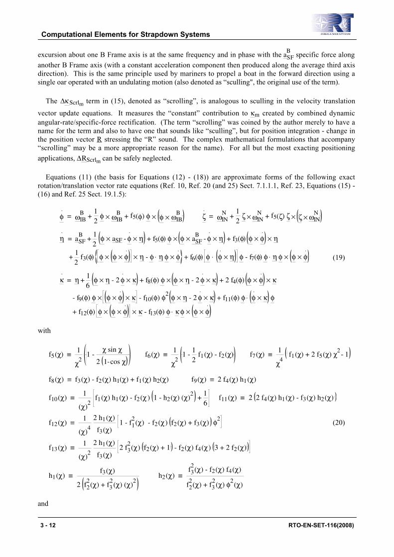
excursion about one B Frame axis is at the same frequency and in phase with the aSFB

specific force along

another B Frame axis (with a constant acceleration component then produced along the average third axisdirection). This is the same principle used by mariners to propel a boat in the forward direction using asingle oar operated with an undulating motion (also denoted as “sculling", the original use of the term).

The Δκ Scrlm term in (15), denoted as “scrolling”, is analogous to sculling in the velocity translation

vector update equations. It measures the “constant” contribution to κm created by combined dynamicangular-rate/specific-force rectification. (The term “scrolling” was coined by the author merely to have aname for the term and also to have one that sounds like “sculling”, but for position integration - change inthe position vector R stressing the “R” sound. The complex mathematical formulations that accompany“scrolling” may be a more appropriate reason for the name). For all but the most exacting positioning

applications, ΔRScrlm can be safely neglected.

Equations (11) (the basis for Equations (12) - (18)) are approximate forms of the following exactrotation/translation vector rate equations (Ref. 10, Ref. 20 (and 25) Sect. 7.1.1.1, Ref. 23, Equations (15) -(16) and Ref. 25 Sect. 19.1.5):

φ = ωIBB +

12

φ × ωIBB + f5(φ) φ × φ × ωIB

B ζ = ωINN +

12

ζ × ωINN + f5(ζ) ζ × ζ × ωIN

N

η = aSFB

+ 12

φ × aSF - φ × η + f5(φ) φ × φ × aSFB

- φ × η + f3(φ) φ × φ × η

+ 12

f3(φ) φ × φ × φ × η - φ ⋅ η φ × φ + f6(φ) φ ⋅ φ × η φ - f7(φ) φ ⋅ η φ × φ × φ (19)

κ = η + 16

φ × η - 2 φ × κ + f8(φ) φ × φ × η - 2 φ × κ + 2 f4(φ) φ × φ × κ

- f9(φ) φ × φ × φ × κ - f10(φ) φ2 φ × η - 2 φ × κ + f11(φ) φ ⋅ φ × κ φ

+ f12(φ) φ × φ × φ × κ - f13(φ) φ ⋅ κ φ × φ × φ

with

f5 (χ) ≡ 1

χ2 1 -

χ sin χ

2 1- cos χ f6 (χ) ≡

1

χ2 1 -

12

f1 (χ) - f2 (χ) f7 (χ) ≡ 1

χ4 f1 (χ) + 2 f5 (χ) χ2

- 1

f8 (χ) ≡ f3 (χ) - f2 (χ) h1(χ) + f1 (χ) h2(χ) f9 (χ) ≡ 2 f4 (χ) h1 (χ)

f10 (χ) ≡ 1

(χ)2

f1 (χ) h1 (χ) - f2 (χ ) 1 - h2 (χ) (χ)2

+ 16

f11 (χ) ≡ 2 2 f4 (χ) h1 (χ) - f3 (χ) h2 (χ)

f12 (χ) ≡ 1

(χ)4

2 h1 (χ)

f3 (χ) 1 - f1

2 (χ) - f2 (χ) f2 (χ) + f3 (χ) φ2

(20)

f13 (χ) ≡ 1

(χ)2

2 h1 (χ)

f3 (χ) 2 f3

2 (χ) f2 (χ) + 1 - f2 (χ) f4 (χ) 3 + 2 f2 (χ)

h1 (χ) ≡ f3 (χ)

2 f22

(χ) + f32

(χ) (χ)2

h2 (χ) ≡ f32

(χ) - f2 (χ) f4 (χ)

f22

(χ) + f32

(χ) φ2 (χ)

and


3 - 12 RTO-EN-SET-116(2008)

φ(t) = φ(τ) dτtm-1

t

φm = φ(tm) ζ(t) = ζ(τ) dτtm-1

t

ζm = ζ(tm)

η(t) = η(τ) dτtm-1

t

ηm = η(tm) κ(t) = κ(τ) dτtm-1

t

κm = κ(tm)

(21)

It is to be noted that the (19) with (20) translation vector rate equations are exact simplified analyticallyequivalent versions of Reference 23, Equations (15) - (16) (based on refined analysis since publication ofReference 23) - However, Equations (19) and (20) are identical to Reference 25, Equations (19.1.5-7) which

were updated after publication of Reference 23. Note also that the η, κ translation vector rates in (19) are

functions of aSFB

and rotation vector rate φ which is a function of inertial angular rate ωIBB

. In Reference 27

using dual-quaternion/screw-vector theory, Wu shows that the velocity translation vector rate is analytically

equivalent to the following further simplified exact version which is a function of aSFB

and angular rate ωIBB

rather than φ:

η = aSFB

+ 12

φ × aSF - ωIBB

× η + f5 (φ) φ × φ × aSFB

- ωIBB

× η - φ × ωIBB

× η + f14 (φ) φ ⋅ η φ × φ × ωIBB

with (22)

f14 (χ) ≡ χ + sin χ

2 χ3 1 - cos χ

- 2

χ4

As of this writing, a further simplified version of the exact position translation vector rate equation in (19)has yet to be found (Ref. 24).

Equations (19) - (22) are analytically exact under general angular-rate/specific-force dynamic conditions.It is easily verified by inspection that under constant B and N Frame inertial angular rate and constant BFrame specific force, the rotation/translation vectors reduce identically to the integrals of the first term in

their respective rate equations (i.e., integrated ωIBB

, ωINN

for φ, ζ, integrated aSFB

for η, and doubly integrated

aSFB

for κ), as they should in light of the discussion at the beginning of this section on their derivation. The

additional terms in these equations (i.e., coning, sculling and scrolling) are small contributions excited bydynamic high frequency inputs (e.g., vibration), and not by lower frequency dynamic inputs that impact theleading terms. For example, in a 7.6 g root-mean-square aircraft vibration environment, Reference 20 (or25), Section 7.4 shows that coning/sculling rates on the sensor assembly could be 9.9 deg/hr and 1.3 milli-gsworst case for a typically mounted INS (compared to lower frequency dynamic maneuver angular-rates/accelerations (e.g., 200 deg/sec and 10 gs) impacting the leading terms). Because theconing/sculling/scrolling terms are small, they can be accurately approximated by simplified versions ofthese terms in Equations (19) - (20). The principal benefit afforded by the use of rotation/translation vectorsin structuring general strapdown navigation equations is that their rate equations can thereby be drasticallysimplified with virtually negligible error (Ref. 23). The utility of the exact rotation/translation raterepresentations in (19) - (22) is to provide a valid exact base from which to formulate simplified versions(e.g., Equations (11)) used for subsequent algorithm development, and as a reference for accuracyassessment of the simplified versions (Ref. 23).


RTO-EN-SET-116(2008) 3 - 13

3.5 Summary of Main Terms Requiring Integration Algorithms

Equations (8), (9) and (10) with (12) - (18) are integral solutions to Equations (3), (6) and (7) over acomputer update cycle. For the most part, they consist of exact closed form expressions fed by the

integrated sensor output terms in Equations (13) - (17). The α, υ integrated angular rate and specific forceacceleration signals in (17) (measured by summing (integrating) angular rate sensor and accelerometerintegrated output increments) are the normal basic inputs to most strapdown inertial system algorithms. TheEquations (13) - (16) terms (coning, sculling, scrolling, doubly integrated accelerometer signals) representfunctions to be implemented by high speed digital computation algorithms operating within the basic mcycle update period.

4. DIGITAL INTEGRATION ALGORITHMS

Digital algorithms in the strapdown system computer are structured to provide integral solutions to theSection 2 differential equations based on repetitive processing at a specified computation rate. The integralsolutions in Section 3 to the Section 2 equations have such a repetitive processing structure, hence, for themost part, are the digital algorithm forms to be programmed directly in the strapdown computer. These areexact solution forms, hence, have no algorithm error if programmed as shown (except for minor trapezoidalintegration algorithm errors for the small/slowly varying terms). Exceptions are the coning, sculling,scrolling and doubly integrated sensor signal integrals in Section 3.4, Equations (13 - (16) needing highspeed digital integration algorithms for implementation. The high speed algorithm errors are a function ofthe high speed digital integration update frequency. Additionally, Taylor series expansion algorithms areneeded for the trigonometric function coefficients in Equations (8), (9) and (10) that avoid singularities

when φm or ζm are near zero. Taylor series truncation error can be designed to be negligible by carryingsufficient terms.

Integration algorithms for the coning, sculling, scrolling and doubly integrated sensor signal terms aretypically designed based on assumed approximate forms for the angular rate and specific force acceleration

history during the computer update period. Commonly assumed forms for ωIBB

and aSFB

are general

polynomials in time:

ωIBB = A0l + A1l t - t l-1 + A2l t - t l-1

2 +

aSFB = B0l + B1l t - t l-1 + B2l t - t l-1

2 + (23)

wherel = High speed computer cycle time index for high speed digital integration algorithms (within the

slower m cycles).

Ail, Bil = Coefficient vectors selected to match the ωIBB

and aSFB

signals from computer cycle l-1 to l.

The high speed updating algorithms can be structured based on truncated versions of Equations (23). Theadvantage of this approach is that the resulting digital algorithms are easily validated by simulation testingusing the truncated forms they have been designed for as inputs. The algorithm solution should match theequivalent result obtained by analytical evaluation of the Section 3.4, Equation (11) integrals under thesame truncated polynomial inputs (Ref. 26 and Ref. 20 (or 25) Sect. 11.1). Exact numerical correspondenceshould be the result for correctly structured and programmed algorithms.

Subsections to follow describe coning, sculling, scrolling and doubly integrated sensor signal digitalintegration algorithms designed to exactly match the Section 3.4, Equations (11) continuous integrals underEquations (23) polynomial inputs truncated after the A1 and B1 terms. Based on the discussion in theprevious paragraph, Reference 26 Section 2.3 describes specialized simulators for validating algorithms of


3 - 14 RTO-EN-SET-116(2008)

this structure. Following subsections also discuss singularity free algorithms for computing the f1 (χ) - f4 (χ)trigonometric functions in Sections 3.1-3.3 and whether orthogonality/normalization corrections are neededfor the attitude algorithms.

4.1 Coning Digital Integration Algorithm

A coning digital computation algorithm for Equation (13) is given by (Ref. 20 (or 25) Sect. 7.1.1.1.1):

ΔφConem = 12

αl-1 + 16

Δαl-1 × Δαl∑l

From tm-1 to tm

αl = Δαl∑l

From tm-1 to tl Δαl = dαt l-1

t l(24)

where

Δαl = Summation of integrated angular rate sensor output increments from cycle l-1 to l.

Equations (24) have been designed to be exact under Equations (23) angular rate input with the ωIBB

polynomial truncated after the A1 term.

4.2 Sculling Digital Integration Algorithm

A sculling digital computation algorithm for Equation (14) is given by (Ref. 20 (or 25) Sect. 7.2.2.2.2):

ΔηSculm = ΔηScull At tm

ΔηScull = 12

α l-1 + 16

Δα l-1 × Δυ l + υ l-1 + 16

Δυ l-1 × Δα l∑l

From tm-1 to tl (25)

υl = Δυl∑l

From tm-1 to tl Δυl = dυt l-1

t l

where

Δυl = Summation of integrated accelerometer output increments from cycle l-1 to l.

Equations (25) have been designed to be exact under Equations (23) angular rate and specific force inputs

with the ωIBB

, aSFB

polynomials truncated after the A1, B1 terms.

Note the similarity in form between the Equations (24) coning algorithm and Equations (25) scullingalgorithm. Reference 14 provides a general formula for deriving the equivalent sculling algorithm (e.g.,Equations (25)) from a previously derived coning algorithm (e.g., Equations (24)).

4.3 Scrolling And Doubly Integrated Sensor Signal Algorithms

Digital algorithms for scrolling computation and doubly integrated sensor signals for Equations (15) -(16) are given by Reference 25, Equations (19.1.11-1) (based on a similar development in Ref. 20 (or 25)Sect. 7.3.3.2 for an alternative scrolling formula):


RTO-EN-SET-116(2008) 3 - 15

ΔκScrlm = δκScrlAl + δκScrlBl∑l

From tm-1 to tm

δκScrlAl = ΔηScull-1 Tl + 12

αl-1 - 112

Δαl - Δαl-1 × ΔSυl - υl-1 Tl

+ 12

υl-1 - 112

Δυl - Δυl-1 × ΔSαl - αl-1 Tl

δκScrlBl = 13

Sυl-1 - 18

Δυ l Tl × Δα l + 16

αl-1 - 34

Δα l + 14

Δα l-1 × υl-1 + 5

12 Δυ l +

112

Δυ l-1 Tl

+ 16

αl-1 - 34

Δα l + 14

Δα l-1 × υl-1 + 5

12 Δυ l +

112

Δυ l-1 Tl (26)

ΔSαl = αl-1Tl + Tl

12 5 Δαl + Δ αl-1 ΔSυl = υl-1Tl +

Tl

12 5 Δυl + Δυl-1

Sυl = ΔSυl∑l

From tm-1 to tl Sυm = Sυl at tm

whereTl = Time interval between computer high speed l cycles.

Equations (26) have been designed to be exact under Equations (23) angular rate and specific force inputs

with the ωIBB

, aSFB

polynomials truncated after the A1, B1 terms.

4.4 Trigonometric Coefficient Algorithms

To assure that no singularities occur when φm or ζm are near zero, the following Taylor series expansion

formulas can be used for the Equations (8), (9) and (10) CBI(m)

BI(m-1), CNI(m-1)

NI(m) , ΔvSFm

Bm-1, ΔRSFm

Bm-1, trigonometric

function coefficients:

f1 (χ) = sin χ

χ = 1 -

χ2

3 ! +

χ4

5 ! - f2 (χ) =

(1 - cos χ)

χ2 =

12 !

- χ2

4 ! +

χ4

6 ! -

(27)

f3 (χ) = 1

χ2 1 -

sin χ

χ =

13 !

- χ2

5 ! +

χ4

7 ! - f4 (χ) =

1

χ2

12

- 1 - cos χ

χ2 =

14 !

- χ2

6 ! +

χ4

8 ! -

Corresponding computational algorithms are then structured from truncated versions of the former. Theseries can be truncated with a sufficient number of terms to assure "error free" performance. For example,

to assure overall eleventh order accuracy in CBI(m)

BI(m-1) (Equations (8)), this would entail carrying f1(χ) out to

tenth order (in φm) and f2(χ) out to eighth order (note, there is no ninth order term in f2(χ) ).

4.5 Orthogonality and Normalization Algorithms

Orthogonality and normalization correction algorithms can be applied to computed direction cosine

matrices (e.g., CBN

and CNE

) to preserve the proper characteristics of their rows and columns (Ref. 20 (or 25)

Sect. 7.1.1.3). Similarly, normalization algorithms can be applied to quaternion attitude representations


3 - 16 RTO-EN-SET-116(2008)

(Ref. 20 (or 25) Sect. 7.1.2.3). One of the advantages in using exact formulated attitude updatingalgorithms (e.g., Equations (8)) is that direction cosines and equivalent quaternion formulations calculatedby integration, will remain orthogonal and normal if initialized as such, independent of sensor error (Ref. 20(or 25) Sect. 3.5.1). Consequently, if computer register round-off error is negligible (as it is for mostapplications using modern day processors), there is no need for orthogonality/normality compensation.

5. STRAPDOWN SENSOR ERROR COMPENSATION

A fundamental problem with all inertial navigation systems is the inability to manufacture inertialcomponents with the inherent accuracy required to meet system requirements. To correct for thisdeficiency, compensation algorithms are included in the INS software for correcting sensor outputs forknown predictable error effects. The compensation algorithms represent the inverse of the inertial sensoranalytical model equations.

This section describes error models and compensation algorithms that can be used to correct for errors inthe strapdown inertial sensors (angular rate sensors and accelerometers), relative displacement betweenaccelerometers (“size effect”), misalignment of the strapdown sensor assembly relative to the system mount,and alignment of the system mount in the user vehicle relative to vehicle reference axes. Included is adiscussion of the application of the sensor compensation algorithms to the Section 4 strapdown inertialnavigation integration routines and their associated coning, sculling, scrolling and accelerometer size-effect/anisoinertia elements.

5.1 Sensor Error Models

This section characterizes the errors typically present in the raw inertial sensor outputs (angular ratesensors and accelerometers) and then describes a general form of compensation equations for correcting theerrors. All vectors in this section are represented in the B Frame, the designation for which has beenomitted for analytical simplicity.

The output vector from strapdown angular rate sensor and accelerometer triads can be characterized as afunction of their inputs as (Ref. 20 (or 25) Sects. 8.1.1.1 and 8.1.1.2):

ωIBPuls = 1

ΩWt0 I + FScal FAlgn ωIB + δωBias + δωQuant + δωRand

aSFPuls = 1

AWt0 I + GScal GAlgn aSF + δaBias + δaSize + δ aAniso + δaQuant + δaRand

(28)

where

ωIBPuls, aSFPuls = Angular rate sensor and accelerometer triad output vector in pulses per second.

Each axis output pulse is a digital indication that the sensor associated with thataxis has received an integrated input increment equal to that particular sensor’spulse size.

ΩWt 0, AWt 0 = Nominal pulse weight (a positive value) for each angular rate sensor (radians per

pulse) and accelerometer (fps per pulse).FScal, GScal = Angular rate sensor and accelerometer triad scale factor correction matrices;

diagonal matrices in which each element adjusts the output pulse scaling tocorrespond to the actual scaling for the particular sensor output. May include non-linear scale factor effects and temperature dependency. Nominally, FScal and GScalare zero.


RTO-EN-SET-116(2008) 3 - 17

FAlgn , GAlgn = Alignment matrices for the angular rate sensor and accelerometer triads. Each row

represents a unit vector along a particular sensor input axis as projected onto theB-Frame. May include specific force acceleration dependency. Nominally,FAlgn and GAlgn are identity.

δωBias, δ aBias = Angular rate sensor and accelerometer triad bias vectors. Each element equals thesystematic output from a sensor under zero input conditions. May haveenvironmental sensitivities (e.g., temperature, specific force acceleration forangular rate sensors, angular rate for accelerometers).

δωQuant, δaQuant = Instantaneous angular rate sensor and accelerometer triad pulse quantization

error vectors associated with the output only being provided when thecumulative input equals the pulse weight per axis.

δωRand, δaRand = Angular rate sensor and accelerometer triad random error output vectors.

δ aSize = Accelerometer triad size effect error created by the fact that due to physical size, theaccelerometers in the triad cannot be collocated, hence, do not measure components ofidentically the same acceleration vector.

δaAniso = Accelerometer triad anisoinertia error effect (present in pendulous accelerometers)

created by mismatch in the moments of inertia around the input and pendulum axes.

References 21 and 20 (or 25) Section 8.1.3 analytically describe the Equations (28) δωQuant, δaQuant

quantization error effects in strapdown inertial sensors. The δaSize size effect term (Ref. 20 (or 25) Sect.

8.1.4.1) and for pendulous accelerometers, the δaAniso anisoinertia term (Ref. 16 and Ref. 20 (or 25) Sect.8.1.4.2), are given by :

δ aSize ≡ GAlgnk

T ⋅ ωIB × l k + ωIB × ωIB × l k uk∑

k=1,3

δaAniso = KAniso ωIBk ωIBkp uk∑k=1,3

(29)

whereuk = Unit vector parallel to the accelerometer k input axis.l k = Position vector from INS navigation center to accelerometer k center of seismic mass.

GAlgnk

T = Vector formed from the kth column of GAlgn

T, the transpose of the GAlgn accelerometer

triad alignment matrixKAniso = Accelerometer anisoinertia coefficient (a generic property of the accelerometer design).

ωIBk, ωIBkp = Angular rate ωIB projections on the accelerometer k input and kp pendulum axes.

5.2 Generic Strapdown Sensor Compensation Forms

The inverse of Equations (28) form the basis for compensating the ωIBPuls, aSFPuls raw sensor outputs to

calculate the true ωIB, aSF angular-rate/specific-force-acceleration inputs for the strapdown inertialintegration operations (Ref. 20 (or 25) Sects. 8.1.1.1 and 8.1.1.2). First, Equations (28) are solved for the BFrame angular rate and acceleration input vector:

ωIB′ = ΩWt0 I + FScal

-1 ωIBPuls

aSF′ = AWt0 I + GScal

-1 aSFPuls

(30)


3 - 18 RTO-EN-SET-116(2008)

ωIB = FAlgn -1 ωIB

′ - δωBias - δωQuant - δωRand

aSF = GAlgn -1 aSF

′ - δaBias - δaSize - δ aAniso - δaQuant - δaRand

(31)

where

ωIB′ , aSF

′ = Scale factor compensated angular rate sensor and accelerometer output vectors.

Equations (30) represent the scale factor compensation equation for the raw angular rate sensor and

accelerometer triad ωIBPuls, aSFPuls outputs. Compensation for the remaining predictable errors in ωIBPuls

and aSFPuls is achieved using a simplified form of (31) in which it is recognized that the δωRand and δaRand

components are unpredictable, hence, can only be approximated by zero:

ωIB ≈ FAlgn -1 ωIB

′ - δωBias - δωQuant

aSF = GAlgn -1 aSF

′ - δaBias - δaSize - δ aAniso - δaQuant

(32)

Compensation Equations (32) are further refined to a more familiar form by introducing the followingdefinitions:

ΩWt ≡ ΩWt0 I + FScal -1 AWt ≡ AWt0 I + GScal

-1

KMis ≡ I - FAlgn -1

LMis ≡ I - GAlgn -1

(33)

KBias ≡ FAlgn -1 δ ωBias LBias ≡ GAlgn

-1 δ a Bias

Substituting (33) into (30) and (32) obtains the equivalent compensation equations:

ωIB′ = ΩWt ωIBPuls

ωIB ≈ ωIB′ - KMis ω′ - KBias - FAlgn

-1 δωQuant

(34)

aSF′ = AWt aSFPuls

aSF ≈ aSF′ - LMis aSF

′ - LBias - GAlgn -1

δaSize + δ aAniso + δaQuant

In many systems, the form of the compensation equations so derived contain linearizationapproximations to the exact inverse relations (to conserve on computer throughput). The approach takenabove is the analytically simpler expedient of using the exact inverse of the complete error model (withoutlinearization approximation) based on the assumption that modern day computers can easily handle theworkload.

5.3 Generic Strapdown Sensor Compensation Algorithms

Equations (34) are the basis for the following algorithms used to form the inputs to the Section 3navigation parameter m cycle updating operations (Ref. 20 (or 25) Sects. 8.1.2.1 and 8.1.2.2):


RTO-EN-SET-116(2008) 3 - 19

α′m = ΩWt αCntm

αm ≈ α′m - KMis α′m - KBias Tm - δαQuantCm

Sαm

′ = ΩWt SαCntm

Sαm ≈ Sαm

′ - KMis Sαm

′ - 12

KBias Tm + δαQuantCm Tm

(35)

υ′m = AWt υCntm

υm ≈ υ′m - LMis υ′m - LBias Tm - δ υSizeCm - δ υAnisoCm - δ υQuantC m

Sυm

′ = AWt SυCntm

Sυm ≈ Sυm

′ - LMis Sυm

′ - 12

LBias Tm + δυSizeCm + δυAnisoCm + δυQuantCm Tm

in which (with Equations (29)) the following definitions apply:

δυSizeCm ≡ GAlgn -1

δ aSize dttm-1

tm

≈ δ aSize dttm-1

tm

= uk ⋅ ωIB × l k + ωIB × ωIB × l k uk dt

tm-1

tm

∑k

δυAnisoCm ≡ GAlgn -1

δ aAniso dttm-1

tm

≈ δ aAniso dttm-1

tm

= KAniso uk ωIBk ωIBkp dttm-1

tm

∑k=1,3

δαQuantCm ≡ FAlgn -1

δωQuant dttm-1

tm

≈ δωQuant dttm-1

tm

(36)

δ υQuantC m ≡ GAlgn -1

δaQuant dttm-1

tm

≈ δaQuant dttm-1

tm

αCntm ≡ dαCnttm-1

tm

υCntm ≡ dυCnttm-1

tmSummation of raw sensor output pulses

over computer cycle m

where

dαCnt, dυCnt = Angular rate sensor and accelerometer instantaneous pulse output vectors.

Reference 20 (or 25) Sect. 8.1.3 (and its subsections) describe various methods for calculating the

δαQuantCm, δ υQuantC m sensor quantization compensation terms. Representative algorithms for the

δ υSizeCm , δ υAnisoCm accelerometer size effect and anisoinertia compensation terms are described next.


3 - 20 RTO-EN-SET-116(2008)

5.3.1 Representative Accelerometer Size Effect And Anisoinertia Computation Algorithms

The size effect and anisoinertia terms in Equations (36) can be calculated at the high speed l cycle ratewithin each m cycle as follows (Ref. 20 (or 25) Sects. 8.1.4.1.1.1 and 8.1.4.2):

βijm ≡ Δαil Δαjl∑l

From tm-1 to tm

δυSizeCYm = fSize - lZ2 ΔαXm - ΔαXm-1 + lX2 ΔαZm - ΔαZm-1

+ lZ2 βYZm + lX2 βXYm - lY2 βZZm + βXXm

δυSizeCZm, δυSizeCXm = Similarly by permuting subscripts.

(37)

δυAnisoCm = fSize KAniso βkpm uk∑k=1,3

wherelik = Component of lk along B Frame axis i.

fSize = Size effect algorithm computation frequency which equals the reciprocal of Tl.

Δαil = Integrated angular rate around B Frame axis i over the l-1 to l computer cycle time interval.

Δαim, Δαim-1 = Δαil for the l-1 to l cycle time intervals immediately preceding the m and m-1 cycle

times.

δυSizeCim = ith B Frame component of δυSizeCm .

The previous algorithm is designed to compute the high frequency dependent terms (βij) at the l cyclerate, use them to calculate size effect at the m cycle rate, and apply the size effect correction at the m cyclerate in Equations (35). This implies that size-effect compensation is not being applied at the l cycle rate,hence, will not be provided on the acceleration data used for high speed sculling calculations (Equations(25)). The associated sculling error is of the same order of magnitude as the basic Equations (37) size-effectcorrection, thus, cannot be ignored. Section 5.4 describes an algorithm for correcting the associated scullingerror at the m cycle rate. Alternatively, the full Equations (37) size-effect correction can be computed and

applied at the high speed l cycle rate with βijm replaced by Δαil Δαjj. The sculling computation would then

be performed with the size-effect compensated accelerometer data, thereby eliminating the previouslydescribed sculling error.

5.4 Compensation Of High Speed Algorithms For Sensor Error

The high speed algorithms described in Sections 4.1- 4.3 and 5.3.1 for coning, sculling, scrolling, doubly

integrated sensor signals, size effect and anisoinertia are based on error free values for the Δαl and Δυlintegrated angular rate sensor and accelerometer increment inputs. This implies that compensated sensorsignals are being used, thereby implying sensor compensation to be performed at the l cycle rate in forming

Δαl and Δυl. The equivalent result can also be obtained by performing the high speed computations withuncompensated sensor data, then compensating the result at the slower m cycle rate. A savings inthroughput can thereby be achieved if needed for a particular application. For the coning algorithm, theassociated operations would be as follows (Ref. 20 (or 25) Sect. 8.2.1.1):


RTO-EN-SET-116(2008) 3 - 21

ΔφConeCntm ≡ 12

αCnt(t) × dαCnttm-1

tm

Δφ ′Conem = ΩConeWt Δ φConeCntm ΔφConem = I - KMisCone Δφ ′Conem

(38)

in which

KMisCone ≡

KMisYY + KMisZZ - KMisYX - KMisZX

- KMisXY KMisZZ + KMisXX - KMisZY

- KMisXZ - KMisYZ KMisXX + KMisYY

(39)

ΩConeWt ≡

ΩWtY ΩWtZ 0 0

0 ΩWtZ ΩWtX 0

0 0 ΩWtX ΩWtY

where

αCnt(t) = α(t) as defined in Equations (11) but based on angular rate sensor output counts.

ΩWti , KMisij = Elements in row i of column i of ΩWt and row i column j of KMis.

Sensor compensation applied at the m cycle rate on uncompensated computed inputs to the accelerometersize effect and anisoinertia routines in Equations (37) would be (Ref. 20 (or 25) Sect. 8.1.4.1.4):

βijm = ΩWti ΩWtj βijCntm Δαim = ΩWti ΔαiCntm (40)

where

βijCntm, ΔαiCntm = βijm, Δαim computed with uncompensated sensor pulse output data.

Similar but more complicated operations are required for post l cycle sculling and scrolling compensationfor sensor error (Ref. 20 (or 25) Sects. 8.2.2.1 and 8.2.3.1). In most applications, however, ignoring sensormisalignment effects in the sculling, scrolling (and size-effect/anisoinertia) calculations introducesnegligible error. Based on this assumption, it then is reasonable to use the direct approach of performing

scale factor compensation on the raw angular rate sensor and accelerometer input data (i.e., applying ΩWtand AWt) at the l cycle rate, and then applying the scale factor compensated signals as input to the sculling,scrolling (and accelerometer size effect/anisoinertia) l cycle computation algorithms (Equations (25), (25)and (37)). However, such an approach can still leave significant error in the sculling/scrolling computationsexecuted using scale factor compensated sensor data without accelerometer size-effect compensation.Reference 20 (or 25), Section 8.1.4.1 shows that the residual sculling error can be accurately approximatedand corrected with:

δΔηScul-SizeCm ≈ 12

α(t) × δaSize + δ υSizeC(t) × ωIB dttm-1

tm

δυSizeC(t) ≈ δaSize dτtm-1

t

(41)

where

δΔηScul-SizeCm = Size effect correction to be applied to a ΔηSculm sculling term calculated with

accelerometer data not containing size effect compensation.


3 - 22 RTO-EN-SET-116(2008)

The δΔηScul-SizeCm correction is applied at the m cycle rate by augmenting the translation vectors in

Equations (12) as follows:

ηm = υm + ΔηSculm - δΔηScul-SizeCm

κm = Sυm + ΔκScrlm - 12

δΔηScul-SizeCm Tm

(42)

Reference 20 (or 25) Section 8.1.4.1.2 shows that δΔηScul-SizeCm in (41) can be accurately approximated by

the following algorithm whose form and magnitude is similar to the basic Equation (37) size-effectcompensation algorithm:

δΔηScul-SizeCYm = fSize 12

αZm Δα′Ym + Δα′Ym-1 lZ1 - Δα′Zm + Δα′Zm-1 lY1

- 12

αXm Δα′Xm + Δα′Xm-1 lY3 - Δα′Ym + Δα′Ym-1 lX3

+ βXXm lY3 + βZZm lY1 - βXYm lX3 - βYZm lZ1 (43)

δΔηScul-SizeCZm , δΔηScul-SizeCXm = Similarly by permuting subscripts.

where

δΔηScul-SizeCim = ith B Frame component of δΔηScul-SizeCm .

Δα′im = ith component of Δαim with only scale factor compensation.

αim = ith component of αm.

The alternative to using (42) with (43) is to apply the Equations (37) size-effect compensation at the highspeed l cycle rate to the scale factor compensated accelerometer data (i.e., using scale factor compensated

Δα l angular rate sensor data for Δαim with βijm replaced by Δαil Δαjj). The sculling computation would

then be performed with the size-effect compensated accelerometer data, thereby eliminating the Equations(41) error effect.

5.5 Compensation For Sensor Triad Attitude Error

The KMis and LMis misalignment error compensation coefficients described in Section 5.2 represent

misalignment of the strapdown sensor axes relative to nominally defined B Frame sensor coordinates. Anadditional misalignment to be compensated in the INS is misalignment of the nominal B Frame relative tothe reference axes of the user vehicle in which the INS is installed.

The attitude of the vehicle in which the strapdown inertial navigation system (INS) is installed is

determined from the attitude direction matrix CBN

, inertial sensor assembly mounting misalignments (relative

to the INS mount), and the orientation of the INS mount relative to user vehicle reference axes. An attitudedirection cosine matrix relating the user vehicle and locally level attitude reference axes can be written as(Ref. 20 (or 25) Sect. 8.3):

CVRFN

= CBN

CBM T

CVRFM

(44)

whereM = INS mount coordinate frame (the B Frame is nominally aligned to the M Frame).


RTO-EN-SET-116(2008) 3 - 23

VRF = User vehicle reference axes.

The CBM

direction cosine matrix can be defined without approximation in terms of the associated rotation

vector components as follows:

CBM

= I + sin J

J J × +

(1 - cos J)

J2 J × 2

(45)

whereJ, J = Sensor triad mount misalignment rotation error vector and its magnitude.

The J components are compensation coefficients measured during system calibration (Ref. 20 (or 25) Sect.

18.4.7.4). The CVRFM

matrix is a function of the particular mount orientation in the user vehicle.

6. STRAPDOWN INERTIAL NAVIGATION ERROR PROPAGATION EQUATIONS

The overall strapdown INS design process requires supporting analyses to develop and verifyperformance specifications. This generally entails the use of a strapdown INS error model in the form oftime rate differential equations that describe the error response of INS computed attitude/velocity/positiondata. Such error models are also fundamental to the design of Kalman filters used, in conjunction withother system inputs, for correcting the INS errors. This section describes strapdown INS error modelequations that represent the INS attitude/velocity/position navigation parameter integration routine responseto sensor errors (i.e., excluding the effect of algorithm and computer finite word-length error, errors that aregenerally negligible in a well designed modern day INS compared to sensor error effects). The term"sensor error" used in this section refers to the residual error in the sensor signals after applying the Section5 compensation corrections. It is only the residual sensor errors that generate INS navigation parameteroutput errors. The residual sensor errors arise from inaccuracy in measuring the sensor compensationcoefficients, sensor random noise outputs that are not accounted for in the compensation algorithms, shortand long term sensor instabilities, and variations in actual sensor performance from the analytical models inSection 5.1 that formed the basis for the sensor compensation algorithms.

6.1 Typical Strapdown Error Parameters

An important part of strapdown INS error model development is the definition (and selection) ofattitude/velocity/position error parameters used in the error model and their relationship to the INSintegration computed navigation parameters (or to a hypothetical set of INS navigation parameters that areanalytically related to the INS computed set). The INS computed navigation parameters described in

Sections 2 - 4 are the CBN

matrix for attitude, the vN vector for velocity, the CNE

matrix for horizontal earth

referenced position, and altitude h for vertical earth referenced position. These contain 20 individual scalarparameters, each of which develop errors in response to sensor error. Furthermore, the 18 error parameters

associated with the CBN

and CNE

matrices (9 elements each) are not independent due to natural

orthogonality/normality constraints that govern all direction cosine matrices. To circumvent the problem ofdealing with the attendant complexities, navigation error is typically described in terms of three navigationerror vectors (for attitude, velocity, and position), each consisting of three independent error components.

The error in the INS computed navigation parameters (in this case, CBN

, vN, CNE

and h) are analytical

functions of the independent error vector parameters. For example, the N Frame components of acommonly used set of attitude, velocity, and position error parameters is (Ref. 20 (or 25) Sects. 12.2.1-12.2.3 and 12.5) :


3 - 24 RTO-EN-SET-116(2008)

ψN× ≡ CEN

I - CBE

CEB

CNE

+ CBN

δαQuantB

×

δVN ≡ CEN

vE

- vE - CBN

δυQuantB

(46)

δRN ≡ CEN

RE

- RE = R CEN

CNE

- I uUpN

+ δh uUpN

where

= Designator for a system computer calculated quantity containing error. The quantity without

the designation is by definition error free (e.g., CBA

is error free and CBA

contains errors).

ψ = Small angle error rotation vector associated with the computed CBE

attitude matrix.

δV = Error in the computed v velocity vector relative to the earth measured in the E Frame.

δR = Error in the computed position vector from earth's center R measured in the E Frame.

δαQuant, δυQuant = Angular rate sensor and accelerometer triad quantization error residual(remaining after applying quantization compensation - Ref. 20 (or 25) Sect.8.1.3 and subsections).

The quantization terms in the ψ and δV equations are included to facilitate differential error equationmodeling (See further explanation at conclusion of Section 6.2 to follow).

An equivalent set of attitude, velocity, position error parameters can also be defined that are more directly

related to the CBN

, vN, CNE

, h navigation parameters computed by direct integration of Equations (1), (6) and

(7) (previous references):

γN× ≡ I - CBN

CNB

+ CBN

δαQuantB

×

δvN ≡ vN

- vN - CBN

δυQuantB

(47)

εN× ≡ CEN

CNE

- I

δh ≡ h - h

where

γ = Small angle error rotation vector in the computed CBN

attitude matrix.

δv = Error in computed velocity measured in the N Frame.

ε = Small angle error rotation vector in the computed CNE

position matrix.

δh = Error in computed altitude.

The two sets of navigation error parameters are analytically related through (previous references):


RTO-EN-SET-116(2008) 3 - 25

ψN = γN

- εN

δVN = δvN + εN × vN (48)

δRN = R εN × uUp

N + δh uUp

N

or the equivalent inverse relationships:

εN =

1R

uUpN

× δRN + εZN uUpN

δh = uUpN

⋅ δRN

(49)

δvN = δVN - εN × vN

γN = ψN

+ εN

where

εZN = Local vertical component of ε (projection on the N Frame Z axis along uUp).R = Distance from earth's center to the current position location (magnitude of R).

6.2 Inertial Sensor Error Parameters

Classical error models for the angular rate sensor and accelerometer triad outputs followingcompensation (in which the error in accelerometer size effect and anisoinertia compensation is ignored asnegligible) are as follows (Ref. 20 (or 25) Sects. 12.4 - 12.5):

δωIBB

= δKScal/Mis ωIBB

+ δKBias + δ ωRand

δaSFB

= δLScal/Mis aSFB

+ δLBias + δaRand

(50)

where

δωIBB

, δaSFB

= Angular rate sensor and accelerometer triad vector error residuals following sensor

compensation but excluding δαQuant, δυQuant quantization compensation errorresiduals.

δKScal/Mis, δLScal/Mis = Residual angular rate sensor and accelerometer scale-factor/misalignment

error matrices remaining after applying ΩWt, KMis, AWt, LMiscompensation in Equations (34).

δKBias, δLBias = Residual angular rate sensor and accelerometer bias error vectors remaining afterapplying KBias, LBias compensation in Equations (34).

Note that the δαQuant, δυQuant quantization compensation error residuals do not appear in the Equations

(50) δωIBB

, δaSFB

error definitions, but instead, show in the Equations (46) - (47) navigation parameter error

vectors. Reference 21 and Reference 20 (or 25) Section 12.5 show that this form results in the navigationerror parameter time rate propagation equations being in standard error state dynamic format (withquantization noise inputs appearing directly, not as their derivatives) as shown next.


3 - 26 RTO-EN-SET-116(2008)

6.3 Error Parameter Propagation Equations

The ψ, δV, δR error parameters defined in Section 6.1 propagate in N Frame coordinates as (Ref. 20 (or25) Sects. 12.3.3 and 12.5.1):

ψN

= - CBN

δωIB B

- ωINN

× ψ N

+ CBN

ωIB B

× δαQuant

δVN

= CBN

δaSFB

+ aSFN

× ψN -

gR

δRHN

+ F(h) gR

δR uUpN

- ωIEN

+ ωINN

× δVN + δgMdlN

- aSF N × CB

N δαQuant - CB

N ωIB

B + ωIE

N × CB

N δυQuant

F(h) = 2 For h ≥ 0 F(h) = - 1 For h < 0 (51)

δRN

= δVN - ωENN

× δRN + CBN

δυQuant

δRHN

= δRN - δR uUpN

δR = uUpN

⋅ δRN

where

δRH, δR = Horizontal and upward vertical components of δR.

δgMdl = Modeling error in g produced by variations in true gravity from the model used in the

system computer.

Equations (51) are based on attitude/velocity/position being updated in the strapdown computer at the samealgorithm repetition rate. For different repetition rates the quantization terms in these equations haverevised coefficients. Note also that the vertical velocity error equations in (51) are different for positivecompared to negative altitudes. This is a manifestation of the difference in gravity model below versusabove the earth's surface (Ref. 20 (or 25) Sect. 5.4).

Equations (51) can be integrated to calculate the response of the attitude, velocity, position errors in astrapdown INS as impacted by accelerometer, angular rate sensor, and gravity model approximation errors.The equations are based on the assumption that the INS navigation parameter integration algorithm errorand computer round-off error is negligibly small.

A similar set of N Frame error propagation equations exist for the Equations (47) γ, δv, ε, δh error

parameters (Ref. 20 (or 25) Sects. 12.3.4 and 12.5.2). Equations (51) for ψ, δV, δR and the equivalent set

for γ, δv, ε, δh can be derived from the differential of any set of strapdown inertial navigation errorpropagation equations (e.g., the set given in Section 2) with the appropriate definitions substituted for thenavigation parameter error terms (e.g., Equations (46) or (47)). Alternatively, Reference 20 (or 25) Section12.3.6 (and subsections) shows that one set of error parameter propagation equations can be derived fromanother by applying the equivalency equations relating the parameters (e.g., Equations (48) or (49)). It isimportant to recognize that the parameters selected to describe the error characteristics of a particular INScan be any convenient set and not necessarily those derived from the navigation parameter differentialequations actually implemented in the INS software. Thus, any set of error propagation equations can beused to model the error characteristics of any INS, provided that the error propagation equations and INSnavigation parameter integration algorithms are analytically correct without singularities over the range ofinterest, and that the sensor error models are appropriate for the application.


RTO-EN-SET-116(2008) 3 - 27

7. CONCLUDING REMARKS

Computational operations in strapdown inertial navigation systems are analytically traceable to basictime rate differential equations of rotational and translational motion as a function of angular-rate/specific-force-acceleration vectors and local gravitation. Modern day strapdown INS computer capabilities allowthe use of navigation parameter integration algorithms based on exact solutions to the differential equations.This considerably simplifies the software validation process and can result in a single set of universalalgorithms that can be used over a broad range of strapdown applications. Exact attitude updatingalgorithms based on direction cosines or an attitude quaternion are analytically equivalent with identicalerror characteristics that are a function of the error in the same computed attitude rotation vector inputs toeach. Modern day strapdown computational algorithms and computer capabilities render the computationalerror negligible compared to sensor error effects.

The angular-rate/specific-force-acceleration vectors input to the strapdown INS digital integrationalgorithms are measured by angular rate sensors and accelerometers whose errors are compensated in thestrapdown system computer based on classical error models for the inertial sensors. Strapdown INSattitude/velocity/position output errors are produced by errors remaining in the inertial sensor signalsfollowing compensation (due to sensor error model inaccuracies, sensor error instabilities, sensor calibrationerrors) and to gravity modeling errors. Resulting INS navigation error characteristics can be defined byvarious attitude, velocity, position error parameters that are analytically equivalent. Any set of navigationparameter error propagation equations can be used to predict the error performance of any strapdown INS.The navigation error parameters used in the error propagation equations do not have to be directly related tothe navigation parameters used in the strapdown INS computer integration algorithms.

REFERENCES

1. Bortz J. E., “A New Mathematical Formulation for Strapdown Inertial Navigation”, IEEE Transactionson Aerospace and Electronic Systems, Volume AES-7, No. 1, January 1971, pp. 61-66.

2. Britting, K. R., Inertial Navigation System Analysis, John Wiley and Sons, New York, 1971.

3. “Department Of Defense World Geodetic System 1984”, NIMA TR8350.2, Third Edition, 4 July 1997.

4. Goodman, L.E. and Robinson, A.R., "Effects of Finite Rotations on Gyroscope Sensing Devices",Journal of Applied Mechanics, Vol. 25, June 1958.

5. Ignagni, M. B., “Optimal Strapdown Attitude Integration Algorithms”, AIAA Journal Of Guidance,Control, And Dynamics, Vol. 13, No. 2, March-April 1990, pp. 363-369.

6. Ignagni, M. B., “Efficient Class Of Optimized Coning Compensation Algorithms”, AIAA Journal OfGuidance, Control, And Dynamics, Vol. 19, No. 2, March-April 1996, pp. 424-429.

7. Ignagni, M. B., “Duality of Optimal Strapdown Sculling and Coning Compensation Algorithms”, Journalof the ION, Vol. 45, No. 2, Summer 1998.

8. Jordan, J. W., “An Accurate Strapdown Direction Cosine Algorithm”, NASA TN-D-5384, September1969.

9. Kachickas, G. A., “Error Analysis For Cruise Systems”, Inertial Guidance, edited by Pitman, G. R., Jr.,John Wiley & Sons, New York, London, 1962.

10. Laning, J.H., Jr., "The Vector Analysis of Finite Rotations and Angles", Massachusetts Institute ofTechnology, Cambridge, Instrumentation Laboratory Special Report 6398-S-3, 1949.


3 - 28 RTO-EN-SET-116(2008)

11. Litmanovich, Y. A., Lesyuchevsky, V. M. & Gusinsky, V. Z., “Two New Classes of StrapdownNavigation Algorithms”, AIAA Journal Of Guidance, Control, And Dynamics, Vol. 23, No. 1,January- February 2000.

12. Mark, J.G. & Tazartes, D.A., “On Sculling Algorithms”, 3rd St. Petersburg International Conference OnIntegrated Navigation Systems, St. Petersburg, Russia, May 1996.

13. Miller, R., “A New Strapdown Attitude Algorithm”, AIAA Journal Of Guidance, Control, AndDynamics, Vol. 6, No. 4, July-August 1983, pp. 287-291.

14. Roscoe, K. M., “Equivalency Between Strapdown Inertial Navigation Coning and ScullingIntegrals/Algorithms”, AIAA Journal Of Guidance, Control, And Dynamics, Vol. 24, No. 2, March-April 2001, pp. 201-205.

15. Savage, P. G., “A New Second-Order Solution for Strapped-Down Attitude Computation”, AIAA/JACCGuidance & Control Conference, Seattle, Washington, August 15-17, 1966.

16. Savage, P. G., “Strapdown Sensors”, Strapdown Inertial Systems - Theory And Applications, NATOAGARD Lecture Series No. 95, June 1978, Section 2.

17. Savage, P. G., “Strapdown System Algorithms”, Advances In Strapdown Inertial Systems, NATOAGARD Lecture Series No. 133, May 1984, Section 3.

18. Savage, P. G., “Strapdown Inertial Navigation System Integration Algorithm Design Part 1 - AttitudeAlgorithms”, AIAA Journal Of Guidance, Control, And Dynamics, Vol. 21, No. 1, January-February1998, pp. 19-28.

19. Savage, P. G., “Strapdown Inertial Navigation System Integration Algorithm Design Part 2 - Velocityand Position Algorithms”, AIAA Journal Of Guidance, Control, And Dynamics, Vol. 21, No. 2,March-April 1998, pp. 208-221.

20. Savage, P. G., Strapdown Analytics, Strapdown Associates, Inc., Maple Plain, Minnesota, 2000.

21. Savage, P. G., "Analytical Modeling of Sensor Quantization in Strapdown Inertial Navigation ErrorEquations", AIAA Journal Of Guidance, Control, And Dynamics, Vol. 25, No. 5, September-October2002, pp. 833-842.

22. Savage, P. G., "Strapdown System Computational Elements", Advances In Navigation Sensors andIntegration Technology, NATO RTO Lecture Series No. 232, October 2003, Section 3.

23. Savage, P. G., "A Unified Mathematical Framework For Strapdown Algorithm Design", AIAA JournalOf Guidance, Control, And Dynamics, Vol. 29, No. 2, March-April 2006, pp. 237-249.

24. Savage, P. G., "Reply by the Author to Y. Wu", AIAA Journal Of Guidance, Control, And Dynamics,Vol. 29, No. 6, November-December 2006, pp. 1485-1486.

25. Savage, P. G., Strapdown Analytics - Second Edition, Strapdown Associates, Inc., Maple Plain,Minnesota, 2007.

26. Savage, P. G., "Performance Analysis Of Strapdown Systems", Low Cost Navigation Sensors andIntegration Technology, NATO RTO-EN-SET-116, October 2008, Section 4.

27. Wu, Y. "Comment on 'A Unified Mathermatical Framework for Strapdown Algorithm Design' ", AIAAJournal Of Guidance, Control, And Dynamics, Vol. 29, No. 6, November-December 2006, pp. 1482-1484.


RTO-EN-SET-116(2008) 3 - 29


3 - 30 RTO-EN-SET-116(2008)