complex methods 1b lent 2010 - the · pdf filecomplex methods 1b lent 2010 february 10, 2010...
TRANSCRIPT
Complex Methods 1B Lent 2010
February 10, 2010
Contents
1 Introduction 3
2 Books 4
3 Analytic Functions 43.1 Complex numbers and the complex plane . . . . . . . . . . . . . . . .. . . . . . . . . 43.2 Complex Valued Functions . . . . . . . . . . . . . . . . . . . . . . . . . .. . . . . . . 53.3 Analytic or holomorphic functions . . . . . . . . . . . . . . . . . .. . . . . . . . . . . 63.4 The Cauchy Riemann Equations . . . . . . . . . . . . . . . . . . . . . . .. . . . . . . 73.5 Some Consequences of the Cauchy Riemann equations . . . . .. . . . . . . . . . . . . 83.6 Harmonic Functions onR2 . . . . . . . . . . . . . . . . . . . . . . . . . . . . . . . . . 113.7 Multi-valued functions, branch points and branch cuts .. . . . . . . . . . . . . . . . . . 123.8 Stereographic Projection and the Riemann Sphere . . . . . .. . . . . . . . . . . . . . . 153.9 Riemann Surfaces . . . . . . . . . . . . . . . . . . . . . . . . . . . . . . . . .. . . . . 173.10 Conformal Mappings . . . . . . . . . . . . . . . . . . . . . . . . . . . . . .. . . . . . 173.11 The line element . . . . . . . . . . . . . . . . . . . . . . . . . . . . . . . . .. . . . . 183.12 The Moebius Map . . . . . . . . . . . . . . . . . . . . . . . . . . . . . . . . . .. . . . 203.13 *Moebius transformations as Lorentz transformations* . . . . . . . . . . . . . . . . . . 223.14 Use of Conformal mappings to solve Laplace’s equation .. . . . . . . . . . . . . . . . 23
4 Cauchy’s Theorem and Contour Integrals 244.1 Some consequences of Cauchy’s Theorem . . . . . . . . . . . . . . .. . . . . . . . . . 254.2 Taylor Series and singularities . . . . . . . . . . . . . . . . . . . .. . . . . . . . . . . 264.3 Taylor-Laurent Expansions . . . . . . . . . . . . . . . . . . . . . . . .. . . . . . . . . 264.4 Classification of singularities . . . . . . . . . . . . . . . . . . . .. . . . . . . . . . . . 284.5 Cauchy’s Integral Formula . . . . . . . . . . . . . . . . . . . . . . . . .. . . . . . . . 294.6 Consequences of Cauchy’s formula . . . . . . . . . . . . . . . . . . .. . . . . . . . . . 30
1
5 Residue Calculus 315.1 Calculating Residues . . . . . . . . . . . . . . . . . . . . . . . . . . . . .. . . . . . . 335.2 Integrating around branch cuts . . . . . . . . . . . . . . . . . . . . .. . . . . . . . . . 345.3 Integrals along the real axis or positive real axis . . . . .. . . . . . . . . . . . . . . . . 345.4 The Keyhole Contour . . . . . . . . . . . . . . . . . . . . . . . . . . . . . . .. . . . . 355.5 Jordan’s Lemma . . . . . . . . . . . . . . . . . . . . . . . . . . . . . . . . . . .. . . . 365.6 Using contour integrals to obtain Cauchy’s Principal Value . . . . . . . . . . . . . . . . 365.7 Contour Integrals used to sum infinite series . . . . . . . . . .. . . . . . . . . . . . . . 38
6 Fourier and Laplace Transforms 396.1 The Fourier Transform . . . . . . . . . . . . . . . . . . . . . . . . . . . . .. . . . . . 396.2 Evaluation of Fourier Transform by Contour Integrationand use of Jordan’s Lemma . . . 406.3 The Fourier Inversion Theorem . . . . . . . . . . . . . . . . . . . . . .. . . . . . . . . 406.4 The Convolution Theorem . . . . . . . . . . . . . . . . . . . . . . . . . . .. . . . . . 416.5 Parseval’s Theorem . . . . . . . . . . . . . . . . . . . . . . . . . . . . . . .. . . . . . 416.6 Solving O.D.E.’s . . . . . . . . . . . . . . . . . . . . . . . . . . . . . . . . .. . . . . 426.7 General Linear Systems . . . . . . . . . . . . . . . . . . . . . . . . . . . .. . . . . . . 426.8 Laplace Transformations . . . . . . . . . . . . . . . . . . . . . . . . . .. . . . . . . . 456.9 Convolution Property . . . . . . . . . . . . . . . . . . . . . . . . . . . . .. . . . . . . 476.10 Inverse Laplace Transform and Bromwich contour . . . . . .. . . . . . . . . . . . . . 496.11 Solution of initial value problems . . . . . . . . . . . . . . . . .. . . . . . . . . . . . . 506.12 Linear Integral Equations and feedback loops . . . . . . . .. . . . . . . . . . . . . . . 506.13 Use of Laplace Transform to solve P.D.E.’s . . . . . . . . . . .. . . . . . . . . . . . . 526.14 Solving the the wave equation using the Laplace Transform . . . . . . . . . . . . . . . . 53
2
1 Introduction
The course is of 16 lectures consisting of four topics of roughly equal duration with emphasis on appli-cations, rather than general theory. Thus the examples are as important as formal theorems. The topicsare
• Analytic (or holomorphic) functions , the main applications are to
a) Solving Laplace’s equation onR2, which is essential for electrostatic and fluid dynamical prob-lems.
b) Conformal Mappings, which may also be used for solving Laplace’s equation but which alsohave applications to many other problems including Cartography.
• Contour Integrals
a) Cauchy’s Theorem as an application of Stokes’s Theorem onR2.
An important application is to
b) The evaluation of real integrals such as
∫ ∞
o
dx
1 + x6,
∫ ∞
o
dx
1 + x3
∫ 2π
0
dθ
(1 + 3 cos2 θ). (1.1)
• Residue Calculuswhich is an algorithm for the evaluation of contour integrals by an examinationof the singularities of the integrand (called in this context theirpoles).
• Fourier and Laplace transformations. The first should be familiar: it allows one to reduce thesolution of ordinary and partial differential equations (O.D.E.’s and P.D.E.’s) to algebra and theevaluation of integrals using the formulae
a) if
F(f(t)) = f(ω) :=
∫ ∞
−∞f(t)e−iωt dt (1.2)
with inverse
f(t) =1
2π
∫ ∞
−∞f(ω)e+iωtdω (1.3)
The evaluation of either (1.2) or (1.3) is often most conveniently effected using contour integration.
b) The Laplace transform is defined by
L(f(t)) = f(s) :=
∫ ∞
0
e−stf(t) dt, s ∈ C (1.4)
and the inversion formula analogous to (1.3) is a contour integral.
3
2 Books
Almost all “mathematical methods ”books contain an accountof most of the material in this course. Onesuch is
G. Arfken and H. Weber,Mathematical Methods for Physicists.Rather more mathematically detailed is
H PriestleyIntroduction to Complex Analysis.
Two other good books are
I Stewart and B. TallComplex Analysis
and
M J Ablowitz and A.S. FokasComplex Variables.
The latter goes somewhat beyond the course.While preparing the lectures I made use of, among others,
E.G. PhillipsFunctions of a Complex Variable.
3 Analytic Functions
3.1 Complex numbers and the complex plane
The special flavour of complex analysis arises because one may think of the complex numbersC bothalgebraicallyas a number system andgeometricallyas a vector space. It is essential therefore to have agood geometrical intuition for the complex plane and so we shall start by briefly reviewing what shouldbe well known.
Complex numbersz are points inR2 with coordinates(x, y) ∈ R × R equipped with a commutative
and associative multiplication law written
z, z′ → zz′ = z′z (3.1)
given by(x, y)(x′, y′) = (xx′ − yy′, xy′ + x′y) (3.2)
We may take1 = (1, 0) andi = (0, 1) as a basis forR2 1 and write
z = x+ iy , with i2 = −1. (3.3)
complex conjugationis reflection in the horizontal axis
(z, y) → (x,−y) = z (3.4)
1In some textbooks for scientists and engineers one seesj used rather thani. Vectors in the complex plane, especially ofthe formejωt, with t being thought of as time are often calledphasorsand represented by arrows which, for positiveω, rotatein an anticlockwise sense as time increases. The complex conjugate of a phasor is an anti-phasor which rotates in a clockwisesense.
4
such thatzz′ = z z′ etc (3.5)
Thenormor modulusof a complex number is defined by
|z| :=√
x2 + y2 =√zz (3.6)
thepositivesquare root being taken. The planeR2 so equipped is called thecomplex planeand denoted
C.On may introducepolar coordinates(r, θ) for C \ 0, they consist of the
modulus r =√
x2 + y2 = |z| , (3.7)
and phase θ = arg z = arctan(y
x) . (3.8)
Obviously, the phaseθ is not defined at the origin(0, 0) because the all radial coordinate linesθ =constant intersect there. Moreover there is some ambiguity in takingthe inverse when definingarctan(y/xIt is also clear, that whatever origin we chose forθ, i.e. whatever radial coordinate lineθ = constant onwhich we setθ = 0,
θ is only defined up to addition of an integer multiple of2π , unless we fix a convention (3.9)
ThePrincipal Valueof the functionarctan(y/x) is defined by
−π < arg z < π (3.10)
We have not definedθ precisely along the negative real axis and it clearly jumps by 2π as we crossthe negative real axis. These elementary observations willbe important later. In the mean time we turnto
3.2 Complex Valued Functions
A complex functionor more precisely acomplex valued functionis just a mapg : C → C, which we mayalso regard as a mapg : R
2 → R2, sending
(x, y) → (u(x, y), v(x, y)) , (3.11)
i.e. z → w = u(x, y) + iv(x, y) = g(z, z) . (3.12)
It is sometimes helpful to think ofw as lying in its own “complexw plane ”. In what follows we mayneed to drop the requirement thatg be defined for allC. It may, for example only be defined in an opensubset ofC. This is done as follows. We have first
Definition An open discD(z0, R) of radiusR centred on some pointz0 given by
D(z0, R) = {z : |z − z0| < R} . (3.13)
Definition An open setU ⊂ C is a (possibly infinite) union or a finite intersection of opendiscs.
5
Sincex =
z + z
2y =
z − z
2i, (3.14)
an equivalent way of specifying a complex valued function is, as indicated in the second equation of(3.12), to usez, z rather thanx, y as coordinates forR2, considered as the domain of the mapg and henceto adopt a notation in whichg as expressed as a function ofz andz. In other words, within its domain ofdefinition, we write
w = u(z + z
2,z − z
2i) + iv(
z + z
2,z − z
2i) := g(z, z) (3.15)
Example
u = x2 − y2 + x , v = 2xy − y (3.16)
g(z, z) = z2 + z (3.17)
By contrast, if we had considered the function
u = x2 − y2 + x , v = 2xy + y (3.18)
we would have hadg(z, z) = z2 + z . (3.19)
3.3 Analytic or holomorphic functions
We see that the expressiong(z, z) giving g will in general contain bothz and z but it can happen thatterms involvingz are absent. Such functions are referred to asanalyticor holomorphic. They are alsosometime as referred to asregular. Intuitively they depend onlyz but not onz. We shall give a precisedefinition shortly. Whatever one calls them, they have many beautiful properties, and from now on weshall mainly work with such functions which we shall write as
z → w = f(z). (3.20)
Of course there is an obvious notion ofanti-analyticor anti-holomorphicfunction obtained by inter-changingz andz, One way to make precise the idea thatf does not depend onz is consider the analogueof thecomplex derivative. Supposeg is defined in a open disc aboutz0. We might consider evaluating
g′(z0) =dg
dz= lim
h→0
(g(z0 + h) − g(z0)
h
)
(3.21)
The problem is that sinceh is an infinitesimal 2-vector, as isg(z0 + h) − g(z0), and we are attempting todivide a vector by a vector and the limit may fail to exist for avariety of reasons e.g.
• g(z) may be ill-defined, for exampleg(z) = 1z2 atz0 = 0.
• more significantlythe limit may depend on the direction in which we take the limit, that is it maydepend onα = arg h.
6
Example g = zdz
dz= lim
h→0
h
h= e−2iα , α = arg h (3.22)
which clearly depends on direction, i.e. onα. We would have similar problems with say
d(zz2)
dz= lim
h→0
(z + h)(z + h)2 − zz2
h(3.23)
but not withd(z2)
dz= lim
h→0
(z + h)2 − z2
h= lim
h→02z + h = 2z . (3.24)
Thus we adopt the following
Definition f(z) is holomorphic or analytic or differentiable in an open discD(z0, R) (or more gener-ally an open setU ⊂ C) if the derivativef ′ exists∀z ∈ U .
Definition f(z) is analytic atz0 ∈ C if there exists a discD(zo, R) such thatf(z) is analytic inD(z0, R).
Definition A functionf(z) is said to be singular atz0 if it not analytic atz0
Definition An entire functionf(z) is one which is analytic in the entire complex plane
Example A polynomial inz is entire . The functionssin z andcos z are entire.It may be proved that if a function is once complex differentiable in a discD(zo, R), then it is infinitely
complex differentiable. Moreover it has a Taylor series in powers ofz, with no z’s, centred onz0 withwhich converges withinD(z0, R). This latter property is often taken as the definition of an analyticfunction. In fact it may be shown that it implies the definition which we have adopted.
3.4 The Cauchy Riemann Equations
Theorem A necessary and sufficient condition thatg(z) = u + iv to be analytic inU ⊂ C is thatu andv have continuous first partial derivatives and and such that
∂u
∂x=∂v
∂y,
∂u
∂y= −∂v
∂x(3.25)
We prove the necessity and omit the sufficiency. Ifh is real we find that
dg
dz=∂u
∂x+ i
∂v
∂x. (3.26)
If h is pure imaginarydg
dz=∂v
∂y− i
∂u
∂y. (3.27)
Equating real and imaginary parts gives the CR equations (3.25).We may make contact with our previous intuitive idea that a holomorphic function depends onz but
not z by defining∂
∂z=
1
2
( ∂
∂x− i
∂
∂y
)
,∂
∂z=
1
2
( ∂
∂x+ i
∂
∂y
)
. (3.28)
7
Thus∂z
∂z= 1 ,
∂z
∂z= 0 ,
∂z
∂z= 1 ,
∂z
∂z= 0 (3.29)
We expect that holomorphic functionf(z) = u+ iv should satisfy
∂f
∂z=
1
2
( ∂
∂x+ i
∂
∂y
)
(u+ iv) = 0 . (3.30)
Equating real and imaginary parts gives (3.25) as expected.
Example Is u = ex cos y the real part of an analytic function? If so, what isv?By the CR equations we must have
∂v
∂y= ex cos y , −∂v
∂x= −ex sin y (3.31)
One checks that mixed partials are equal and integrates
v = ex sin y + function of x (3.32)
v = ex sin y + function of y (3.33)
Thusf = ex(cos y + i sin y) = ex+iy + constant = ez + constant (3.34)
Example Is zz analytic ?
u = x2 + y2 , v = 0 , (3.35)
and the CR equations (3.25) are not satisfied.
3.5 Some Consequences of the Cauchy Riemann equations
Cor.1 (i) The productgf and (ii) the the compositionr = g ◦ f of two holomorphic maps is holomorphicBoth properties are intuitively obvious but we can prove them formally using the CR equations (3.25)
.
(i) If f(z) = u(x, y) + iv(x, y) andg(z) = s(x, y) + it(x, y), then
gf = (us− vt) + i(vs+ ut) (3.36)
Leibniz and the CR equations foru, v ands, t show that(us − vt) and(vs + ut) also satisfy the CRequations
(ii) We havew = f(z) = u(x, y) + iv(x, y) , r = g(w) = s(u, v) + it(u, v) (3.37)
the composition is
r(z) = g ◦ f == g(f(z)) (3.38)
= s(u(x, y), v(x, y)) + it(u(x, u), v(x, y)) (3.39)
8
The chain rule gives
∂xs = ∂us ∂xu+ ∂vs ∂xv (3.40)
∂yt = ∂ut ∂yu+ ∂vt ∂yv (3.41)
But
∂us = ∂vt , ∂vs = −∂ut , (3.42)
∂xu = ∂yv , ∂yu = −∂xv (3.43)
Thus∂xs = ∂yt (3.44)
A similar argument shows that∂ys = −∂xt (3.45)
Cor.2 The level setsu = constant andv = constant are orthogonal.
The normals are∇u = (∂xu, ∂yu) , ∇v = (∂xv, ∂yv) (3.46)
Thus
∇u.∇v = ∂xu∂xv + ∂yu∂yv (3.47)
= ∂yv∂xv − ∂xv∂yv = 0 , (3.48)
by the CR equations (3.25).
Cor.3
|∇u|2 = |∇v|2 =∣
∣
df
dz
∣
∣
2(3.49)
On has by (3.25)|∇u|2 = (∂xu)
2 + (∂y)2 = (∂xv)
2 + (∂yu)2 . (3.50)
Moreover
df
dz=
1
2(∂x − i∂y)(u+ iv) (3.51)
=1
2
(
∂xu+ ∂yv + i(∂xv − ∂yu))
(3.52)
= ∂xu− i∂yu (3.53)
= ∂yv + i∂xv (3.54)
(3.55)
Cor.4 The Jacobian∂(u,v)∂(x,y)
of the map is positive, i.e. the map preserves orientation
9
∂(u, v)
∂(x, y)=
∣
∣
∣
∣
∣
∣
∣
ux uy
vx vy
∣
∣
∣
∣
∣
∣
∣
= v2x + v2
y = |∇v|2 = u2x + u2
y = |∇u|2 . (3.56)
Definition A closed curvez = γ(t) is one for which there is some least valueT > 0 for whichγ(t) = γ(t + T ), ∀ t ∈ R. A simple closed curvez = γ(t) is one for which ifz(t1) = z(t2) with|t2 − t1| < T impliesti = t2 .
That is a simple closed curve does not intersect itself. Thought of as a continuous map from the circleS1 to the planeγ : S1 → R
2 it is 1 − 1 on its image. We shall often, but not always, chose the parametert along the curve such thatT = 2π and restrict the parameter to lie in the interval0 ≤ t ≤ 2π.
The Jordan Curve Theorem States that a simple closed curveγ bounds a domainD topologicallyequivalent ( i.e. continuously deformable) to the unit disc|z| < 1 and such thatγ = ∂D maps to the unitcircle |z| = 1
In what follows,we shall usually assume that the direction of increasingt is chosen so that the domainD is on one’s left hand side ast increases, as it it would if one traversed the unit circle in the direction ofincreasingθ.
The positivity of the Jacobian (3.56) has the important consequence that if one follows a simple closedcurveγ(t) = ∂D given say by a complex valued periodic function oft
z = z(t) = x(t) + iy(t) , z(t) = z(t+ 2π) (3.57)
in thez-plane with the insideD on ones left hand side ast increases . The imagew = w(t) = f(γ =f(z(t)) in the w-plane will be a closed curvef(γ) and if it is simple, then the insidef(D) will also beon one’s left hand side ast increases.
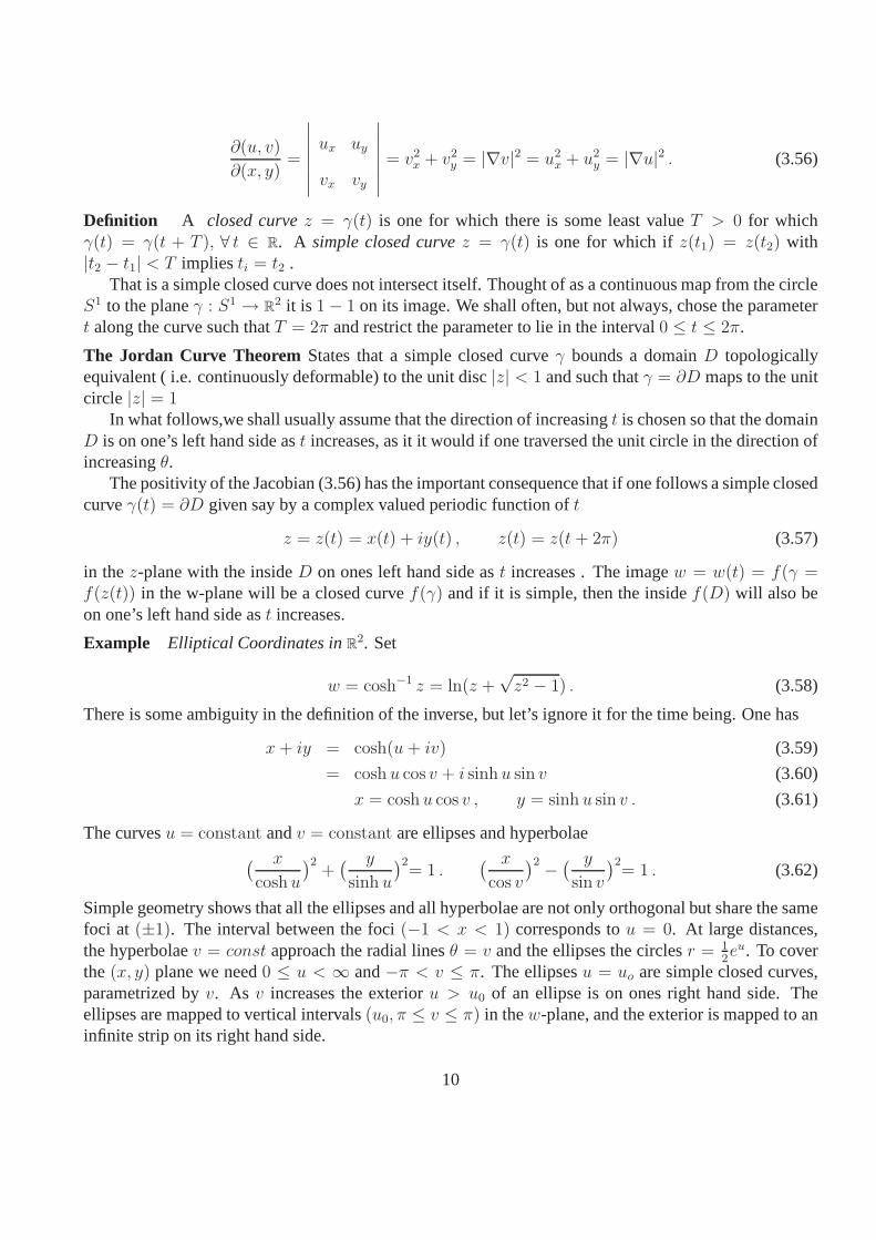
Example Elliptical Coordinates inR2. Set
w = cosh−1 z = ln(z +√z2 − 1) . (3.58)
There is some ambiguity in the definition of the inverse, but let’s ignore it for the time being. One has
x+ iy = cosh(u+ iv) (3.59)
= cosh u cos v + i sinh u sin v (3.60)
x = cosh u cos v , y = sinh u sin v . (3.61)
The curvesu = constant andv = constant are ellipses and hyperbolae( x
cosh u
)2+
( y
sinh u
)2= 1 .
( x
cos v
)2 −( y
sin v
)2= 1 . (3.62)
Simple geometry shows that all the ellipses and all hyperbolae are not only orthogonal but share the samefoci at (±1). The interval between the foci(−1 < x < 1) corresponds tou = 0. At large distances,the hyperbolaev = const approach the radial linesθ = v and the ellipses the circlesr = 1
2eu. To cover
the (x, y) plane we need0 ≤ u < ∞ and−π < v ≤ π. The ellipsesu = uo are simple closed curves,parametrized byv. As v increases the exterioru > u0 of an ellipse is on ones right hand side. Theellipses are mapped to vertical intervals(u0, π ≤ v ≤ π) in thew-plane, and the exterior is mapped to aninfinite strip on its right hand side.
10
3.6 Harmonic Functions onR2
Definition A Harmonic functionφ(x, y) onR2, or possibly a open subset or domainD ⊂ R
2, is a realvalued function satisfying Laplace’s equation
∇2φ = ∂2xφ+ ∂2
yφ = 0 . (3.63)
Clearly we needφ to be suitably smooth. Having continuous second partial derivatives is certainlysufficient for our definition to make sense. We have the following important
Proposition The real and imaginary parts of a functionf(z) which is analytic inD are harmonic.Conversely, given a harmonic functionφ(x, y) , there is a so-called conjugate harmonic functionψ(x.y)with orthogonal level sets such thatf = φ+ iψ is analytic inD.
The proof in one direction is a straight forward consequenceof the CR equations(3.25) and the equal-ity of mixed partials. One has
∂2xu = ∂x∂yv = ∂y∂xv = −∂2
yu, (3.64)
Similarly for v. Alternatively we have∂
∂zf(z) = 0 (3.65)
Thus
∂2
∂z∂zf(z) =
1
4(∂x − i∂y)(∂x + i∂y)f =
1
4
(
∂2x + ∂2
y − i∂y∂x + i∂x∂y
)
f =1
4∇2f = 0 . (3.66)
Now take real and imaginary parts of (3.66) .Converselygiven a harmonic functionφ(x, u), set
f(z) = φ+ iψ (3.67)
for someψ(x, y) to be found, and impose the CR equations (3.25)
∂xψ = −∂yφ ∂yψ = ∂xφ (3.68)
The integrability condition for the exact differential
dψ = −φydx+ φxdy (3.69)
is precisely Laplace’s equation (3.66).Alternatively, we can use the notation of vector analysis. We haveto solve
∇ψ = A (3.70)
whereA = (−∂yφ, ∂xφ, 0) (3.71)
The integrability condition is
curlA = ∇×A (3.72)
=
∣
∣
∣
∣
∣
∣
∣
∣
∣
∣
i j k
∂x ∂y ∂z
−∂yφ ∂xφ 0
∣
∣
∣
∣
∣
∣
∣
∣
∣
∣
(3.73)
= (0, 0, ∂2xφ+ ∂2
yφ) = 0 . (3.74)
11
Examplee
za = e
xa cos(
y
a) + ie
xa sin(
y
a) , a ∈ R (3.75)
These two solutions , together others obtained frome−za ande±i z
a give the solutions one would obtain ifone separates variables, i.e. makes theansatz
φ(x, y) = g(x)h(y) (3.76)
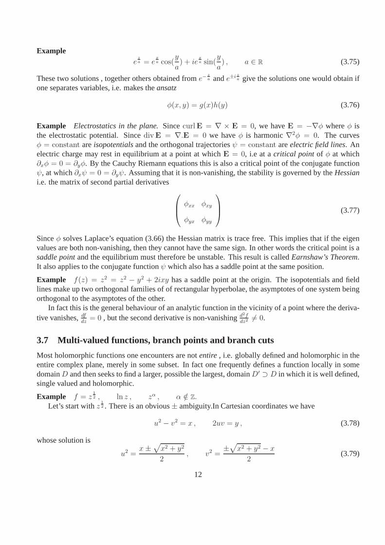
Example Electrostatics in the plane.SincecurlE = ∇ × E = 0, we haveE = −∇φ whereφ isthe electrostatic potential. Sincediv E = ∇.E = 0 we haveφ is harmonic∇2φ = 0. The curvesφ = constant areisopotentialsand the orthogonal trajectoriesψ = constant areelectric field lines. Anelectric charge may rest in equilibrium at a point at whichE = 0, i.e at acritical point of φ at which∂xφ = 0 = ∂yφ. By the Cauchy Riemann equations this is also a critical point of the conjugate functionψ, at which∂xψ = 0 = ∂yψ. Assuming that it is non-vanishing, the stability is governed by theHessiani.e. the matrix of second partial derivatives
φxx φxy
φyx φyy
(3.77)
Sinceφ solves Laplace’s equation (3.66) the Hessian matrix is trace free. This implies that if the eigenvalues are both non-vanishing, then they cannot have the same sign. In other words the critical point is asaddle pointand the equilibrium must therefore be unstable. This resultis calledEarnshaw’s Theorem.It also applies to the conjugate functionψ which also has a saddle point at the same position.
Example f(z) = z2 = z2 − y2 + 2ixy has a saddle point at the origin. The isopotentials and fieldlines make up two orthogonal families of of rectangular hyperbolae, the asymptotes of one system beingorthogonal to the asymptotes of the other.
In fact this is the general behaviour of an analytic functionin the vicinity of a point where the deriva-tive vanishes,df
dz= 0 , but the second derivative is non-vanishingd2f
dz2 6= 0.
3.7 Multi-valued functions, branch points and branch cuts
Most holomorphic functions one encounters are notentire, i.e. globally defined and holomorphic in theentire complex plane, merely in some subset. In fact one frequently defines a function locally in somedomainD and then seeks to find a larger, possible the largest, domainD′ ⊃ D in which it is well defined,single valued and holomorphic.
Example f = z12 , ln z , zα , α /∈ Z.
Let’s start withz12 . There is an obvious± ambiguity.In Cartesian coordinates we have
u2 − v2 = x , 2uv = y , (3.78)
whose solution is
u2 =x±
√
x2 + y2
2, v2 =
±√
x2 + y2 − x
2(3.79)
12
We may fix this± ambiguity by demanding thatu2 andv2 are real and positive
u2 =x+
√
x2 + y2
2, v2 =
√
x2 + y2 − x
2(3.80)
We thus have
u = ±
√
√
x2 + y2 + x
2, v = ±
√
√
x2 + y2 − x
2(3.81)
There is apparently a choice of four possible sign combinations but from the second equation of (3.78),if y > 0, the two signs must be taken to be the same, and ify < 0 they must be taken to be opposite.
We can fix the sign ofu so that the square root is positive on the real axis. This gives what is calledonebranchof the functionz
12 . If we decide thatz
12 is negative on the real axis we get the other branch.
This, slightly complicated, situation can be simplified by passing to polar coordinates. We have
z12 = r
12 e
12iθ (3.82)
Since, however we defineθ, we cannot fix it globally to better than the addition of an integral multiple of2π, we cannot expect thatz
12 to be globally better defined than up to a factor of±1. If we adopt what we
called earlier theprincipal branchfor θ−π < θ < π (3.83)
we have
−π2<θ
2<π
2(3.84)
This z12 = i just above the negative real axis andz
12 = −i just below the real axis. In order to obtain
a domainD in which z12 is single valued and holomorphic wecut or slit the complex plane along the
negative real axis(x ≤, 0). That is, we omit the negative real axis, and choose the domainD′ = C\ (x ≤0, 0). The negative real axis is referred to as abranch cut, and it includes, and ends on, the origin2 ,which is referred to as abranch point. A formal definition will be given shortly.
The function so-defined maps the cutz-plane onto the right handw-plane, i.e ontou = ℜw > 0.This is equivalent to using the upper sign forv in (3.81) wheny is positive and the lower sign wheny isnegative.
If we had chosen the lower sign in (3.81) wheny is positive and the upper sign wheny is negative,we should have obtained a different branch of the functionz
12 which maps the cutz-plane to the left hand
w-plane,i.e. tou = ℜw < 0.
Example log z. We introduce polars:
log z = log r + iθ. (3.85)
There are clearly infinitely many possible branches of the logarithm function. If we cut thez-plane alongthe negative real axis and take the principal branch forθ we get a map ofD′ = C \ (x ≤ 0, 0) into thestrip(−∞ < u <∞,−π < θ < π) . The other branches mapC\ (x ≤ 0, 0) into parallel strips displacedvertically by integer multiples of2π.
2i.e. it is the non-positive real axis
13
Example zα. We introduce polarszα = rαeiαθ (3.86)
and cut as before. Ifα is rationalα = p/q with p and q relatively prime, there will beq branches.Otherwise there will be infinitely many.
Example
(z2 − 1)12 = (r1r2)
12 exp i(
θ1 + θ22
) (3.87)
with z − 1 = r1eiθ1 , z + 1 = r2e
iθ2 .Consider what happens if we move in the complex plane around asimple closed curve. Now
• eiθ12 is 2-valued if we encirclez = 1.
• eiθ22 is 1-valued if we encirclez = 1
• eiθ12 is 1-valued if we encirclez = −1
• eiθ22 is 2-valued if we encirclez = −1
• ei(θ1+θ2
2) is single valued if we encircle bothz = 1 andz = −1 or neither.
We have at least two options for cutting. One is to cut fromz = −1 to z = +1 along the real axis.The other is to introduce two cuts from, one from−∞ to −1 along the real axis, and the other from1 to+∞ along the real axis. In both cases there at two branch points at z = ±1. Let’s take the first option,slitting the plane from−1 to +1 along the real axis. If we than take the principal branches for θ1 andθ2.(z2 − 1)
12 will then be real and positive on the positive real axis and real and negative on the negative real
axis. Just above the cut we have(z2 − 1)12 = i
√r1r2 and just below the cut(z2 − 1)
12 = −i√r1r2. The
function(z2 − 1)12 so defined has a discontinuity of2i
√r1r2across the cut (moving downwards).
To give a definition of a branch point we need to introduce the notion of a simply connected domain
Definition An open domainD ⊂ C is said to besimply connectedif every continuous closed curveγ ⊂ D can be continuously shrunk to a point, through a family of curves lying entirely withinD.
Definition We sayz0 is not a branch point of a functionf(z) if there exists a simply connected domainD containingz0 such that its restrictionf|γ = f(γ(t)) to any closed curveγ(t) ⊂ D is single valued.Otherwise we say thatz0 is a branch point.
Definition We say thatf(z) has a branch point at infinity if it is not single valued aroundall sufficientlylarge curves.
Example (z2 − 1)12 does not have a branch point at infinity
Example (z3 − 1)12 has three branch points atz = z = ei 2∂
3 andz = e−i 2∂3 . It also has a branch point
at infinity.While there is no ambiguity in locating branch points, thereis some arbitrariness in selecting a set of
branch cuts as we have seen. The criterion for a successful choice is that once they have been removed,the resultant function is single valued, at the expense of being discontinuous across the cuts.
Example The International Date LineTo understand this, and to clarify what is happening at infinity, it is convenient to consider
14
3.8 Stereographic Projection and the Riemann Sphere
Consider a unit sphereS2 in 3-dimensional Euclidean space given say by
x2 = x21 + x2
2 + x23 = 1 , (3.88)
with its south pole (SP) (i.e.x = (0, 0,−1) ) resting on (i.e. tangent to ) the planeΠ given byx3 = −1.We may map all pointsx ∈ S2 except the north pole (NP) (i.e.x = (0, 0,+1) ). onto the plane by contin-uing the straight line from the north pole through the pointx onto the planeΠ. If φ is azimuth (i.e. angleof rotation about the diameter joining the NP and SP) andβ co-latitude (i,e. the angle measured from theNP) then with a suitable choice of origin and scale the image of x = (sin β cosφ, sin β sinφ, cosβ) 3 onthe planeΠ is given by
z = x+ iy = eiφ cot(β
2) . (3.89)
Thusφ = θ modulo integer multiples of2π.
Definition The mapS2 \ NP → C is calledstereographic projection from the north pole
Intuitively the NP pole maps to infinity in the complex planeC and we can think of the sphere as thedisjoint union of the planeΠ and a point at infinity∞
S2 = Π ⊔∞ (3.90)
We could just as well have considered the planeΠ given byx3 = +1 tangent to the north pole.Stereographic projection from the south pole takesS2 \ SP to Π. Thus
S2 = Π ⊔ ∞ (3.91)
If we introduce a complex coordinatez on Π then for a suitable choice of origin and scale we have
z =1
z(3.92)
Now considerΠ × Π with coordinates(z, z). If we call Γ the mapC \ 0 → C \ 0 given by (3.92) we seethat
S2 = C × C/Γ (3.93)
Note that
SP ≡ z = 0 ≡ z = ∞ , (3.94)
SP ≡ z = 0 ≡ z = ∞ . (3.95)
DefinitionThe resultant completion of the complex numbers is called theRiemann Sphere
3In many books(φ, θ) are used for azimuth and co-latitude. Sinceθ is standard for plane polars, we don’t have that option.
15
Example Theantipodal map
φ→ −φ , β → π − β (3.96)
or
z → −1
z(3.97)
is anti-holomorphic, orientation reversing, and fixed point free.The long and short of this discussion is that to check for branch points at infinity we use (3.92) to
introduce the coordinatez and examine the pointz = 0
Example
f(z) = (z3 − 1)12 = z−
32 (1 − z3)
12 (3.98)
There is a branch point atz = 0, i.e. at infinity. as well as atz = 1 andz = e±i 2π3 , i.e. z = 1 and
z = e∓i 2π3
Branch cuts can be taken betweenz = 1 andz = ∞ along the real axis and betweenz = e±i 2π3 .
Example
f = z12 =
1
z12
(3.99)
This has a branch point at both the north and the south pole. Wecan run a branch cut along a meridianfrom pole to pole.
Example
f = (z2 − 1)12 =
1
z(1 − z2)
12 (3.100)
Sincef → 1z
at infinity (i.e for smallz) , f has a singularity at infinity ( in fact a pole ) but it isnotabranch point.
Example The International DatelineIf z = eiθ cot(β
2) we letθ = 0 be the Greenwich meridian, then local time is given by
ℑ log z = ℜw ,w = − log z (3.101)
and increase as we go eastward and decreases as we go westward. There are branch points at thenorth and south pole and by international convention a branch cut is drawn connecting the two. A glanceat an atlas will reveal that although this is a perfectly respectable branch cut it is not, for very practicalreasons, always along the meridianφ = θ = 180◦. 4.
DefinitionThe function
w = f(z) = −i log z (3.102)
mappingS6 \NP ⊔ SP to the infinite strip−πu ≤ π, −∞ < v ≤ ∞ is calledMercator’s projection.
4see http://www.phys.uu.nl/˜vgent/idl/idl.htm for details
16
3.9 Riemann Surfaces
Rather than deal with a function with many branches,fi(z) in other words a collection of functionsfi(z),i = 1, 2, . . . , n defined onn identical domains,Ui , whose boundaries∂Ui consist of a set of branch cuts,it is sometimes more convenient to think of a single functiondefined on a single domainΣ = ⊔i=n
i=1Ui
where the overline indicates that the domainsU are glued together across their common boundary branchcuts.
This can give rise to a topologically complicated object, especially if one adds in the points at infinity.The resultant construction is called ann-sheeted Riemann surface, the domains or cut planesUi beingthesheets. A detailed discussion is beyond the scope of this course.
One way to think of a Riemann surface, is to consider the subset
(z, w) = (z, f(z)) (3.103)
of C × C ≡ R4 asz varies over the complex plane or if we add the point at infinityover the Riemann
sphere. One obtains in this way a two real dimensional surface or manifold in four-dimensional Euclideanspace. It is a pleasing exercise (but far beyond the scope of this course) to show that this surface is like asoap film: it extremizes surface area.
3.10 Conformal Mappings
A general linear mapR2 → R2
x
y
→
α β
γ δ
x
y
α, β, γ, δ ∈ R (3.104)
=⇒ w = w1
2(α+ iγ − iβ + δ)z +
1
2(α + iγ + iβ − δ)z (3.105)
is not holomorphic. For example ifβ = γ = 0, we get a diagonal matrix which expands thex coordinateby a factorα and they coordinate by a factorδ. If α 6= δ this will change the angles that lines through theorigin make with the axes and with each other. Circles are taken to to ellipses. Squares with sides parallelto the axes are taken into rectangles with sides parallel to the axes, but a rectangle or even a square whosesides are not parallel to the axes will be taken to a general parallelepiped. Such transformations are calledshears. By contrast a linear holomorphic map is just the composition of a rotation and a dilatation andthus preserves angles, and takes circles to circles, and rectangles to rectangles.
For a general map we need to consider infinitesimal rectangles, or better the angles between curves.
Definition The tangent vectorT of a curvez = γ(t) in thez-plane is
T =dγ
dt=dz
dt=dx
dt+ i
dy
dt= x+ iy (3.106)
Definition The length of the tangent vector is
|T | =√
x2 + y2 =∣
∣
dγ
dt
∣
∣ (3.107)
17
DefinitionGiven two such curves,γ1 andγ2 , the angleα between them is given by
eiα =T1
T2
|T2||T1|
(3.108)
Now consider a general holomorphic map from an open set in thez-plane into an open set in the thew -plane
w = f(z) (3.109)
It will map a curvez = γ(t) in thez-plane to a curvew = γ(t) = f(γ(t)) in thew-plane. The tangentvector is
T =dγ
dt=dw
dt=df
dz
dz
dt=df
dzT (3.110)
The angle between the two curvesγ1(t) andγ2(t) is given by
eiα =T1
T2
|T2||T1|
= eiα . (3.111)
DefinitionA mapping from an open subset ofR
2 to an open subset ofR2 which preserves the angles betweencurves is is calledconformal.
From (3.110) it follows that the effect of an analytic mapping on a infinitesimal vector atz in thez-plane is to take it to an infinitesimal vector atw = f(z) in thew- plane which ismagnifiedby anamount|f ′| and rotated through an anglearg f ′. Thus an infinitesimal rectangle of sidesdx anddy istaken into and infinitesimal rectangle of sidesdu anddv which is both magnified and rotated, but itremains a rectangle. If we think ofdw as the infinitesimal displacement resulting from an infinitesimaldisplacementdz we have
dw = f ′(z)dz (3.112)
If the map were not conformal, then an infinitesimal rectangle would be mapped into a infinitesimalparallelepiped, that is it would suffer ashear.
3.11 The line element
Pythagoras’s theorem tells us that the the infinitesimal distanceds 5 between(x, y) and(x+ dx, y + dy)is given by
ds2 = dx2 + dy2 = dzdz (3.113)
In general curvilinear coordinates(u, v) say we have
d2s = E(u, v)du2 + 2F (u, v)dvdu+G(u, v)dv2 (3.114)
5One can of course easily avoid the use of the language of infinitesimals if one wishes, but it simplifies notation consider-ably,is intuitively clear, and universally used
18
for some functionsE,F,G which are often assembled into a symmetric matrix
E F
F G
(3.115)
and referred to as a “metric tensor ”. The expression (3.114)is referred to asthe line element. The angleα between the coordinate lines is given by
cosα =F√EG
(3.116)
The expression (3.114) also holds for the infinitesimal distance on a curved surface. It can be used notonly to work out distances but angles and areas as well.
In the case of a holomorphic mappingw = f(z) we have
dwdw = |f ′(z)|2dzdz (3.117)
thus all infinitesimal lengths inw-plane are scaled by a factor|f ′| as we saw above.
Example Elliptical coordinates in the planeFrom(3.58)w = f(z) = cosh−1 z
ds2 = dzdz = | sinhw|−22dwdw =1
cosh2 u− cos2 v
(
du2 + dv2)
. (3.118)
Example The SphereThe line element for the standard unit sphereS2 : x(β, φ) = (sin β cos φ, sinβ sinφ, cosβis given by
ds2 = dx.dx = dβ2 + sin2 βdφ2 . (3.119)
Note that the coordinate linesφ = constant, themeridiansand the coordinate linesβ = constant thecircles of latitudeare orthogonal.
Using the formula for stereographic projection we have
4dzdz
(1 + zz)2= dβ2 + sin2 βdφ2 . (3.120)
From this one deduces
Proposition Stereographic projection is conformalMoreover the composition of angle preserving maps is angle preserving, and we deduce from (3.102)
that
Proposition Mercator’s projection is conformalIn Mercator’sw-plane, a straight line makes a constant angle with the the vertical linesu = constant
But these are are the images of the meridians.
Definition A rhumb lineor loxodromeon the sphere is a curve making a constant angle with themeridians.
Thus
19
Proposition Rhumb lines map to straight lines under Mercator’s projection.
Definition A circle on the sphere is the intersection of the sphere with aplane. If the plane passesthrough the centre is is calledgreat circle, otherwise asmall circle. One has the following
Proposition Stereographic projection maps circles to circles.Recall that ifβ, φ are polar coordinates, the unit sphere in Euclidean space isgiven
x21 + x2
2 + x23 = 1 , (3.121)
x+ix2 = sin βeiφ , x3 = cosβ . (3.122)
A plane with unit normaln is given by
x1n1 + x2n2 + n3x3 = p , (3.123)
and will intersect the sphere providedp2 ≤ 1. If n = ni + in2, then simple calculation starting from theformula for stereographic projection (3.89) converts (3.123) to the form
∣
∣
∣z +
n
n3 − p
∣
∣
∣
2
=1 − p2
(n3 − p)2. (3.124)
Now (3.124) is the formula for a circle of centre− nn3−p
and radius√
1−p2
|n3−p| . If n3 = p the plane (3.123)contains NP and and the projection is the straight line
zn + zn = 2p . (3.125)
It follows that if two circles, either of which may great or small, intersect on the sphere with a cer-tain angle, their stereographic projections will be circles or straight lines which intersect at the sameangle. These fact were well known to Hipparchus who established then using classical Euclidean geom-etry. They are at the basis of all subsequent applications ofstereographic to astronomy, crystallography,geology etc, etc.
3.12 The Moebius Map
This is a 1-1 map of the Riemann sphere to itself given by
z → w =az + b
cz + d, ad− bc 6= 0 . (3.126)
Note thata, b, c, d andλa, λb, λc, λd λ 6= 0 give the same Moebius transformation and so one oftenimposes the condition
ad− bc = 1 . (3.127)
This doesn’t fixa, b, c, d completely becausea, b, c, d and−a,−b,−c,−d both satisfy (3.127) but givethe the same Moebius transformation. However the condition(3.127) does show that there is a six real orthree complex parameter’s worth of Moebius transformations. As a consequence we have
20
Proposition Any three distinct assigned pointsz1, z2, z3 may be mapped to any other three disinctassigned pointsw1, w2, w3 by a Moebius transformation.Since Moebius transformations form a group itis sufficient to takew1, w2, w3 = 1, 0,∞ by
w =(z − z1)(z2 − z3)
(z − z3)(z2 − z1). (3.128)
If w1, w2, w3 6= 1, 0,∞ we then compose with the inverse
w =zw3(w2 − w3) + w1(w3 − w2)
z(w2 − w1) + (w3 − w2). (3.129)
which takes0, 1,∞ tow1, w2, w3
Example Examples of Moebius transformations
w = eiαz α ∈ R a rotation (3.130)
w = kz k ∈ R a dilation (3.131)
w = z + a k ∈ C a translation (3.132)
w = az + b a, b ∈ C , a general affine map (3.133)
w = 1/z an inversion (3.134)
Now from (3.126)
w =a
c+bc− ad
a
1
cz + d, c 6= 0 (3.135)
let
f1(z) = cz + d a shear − free affine map (3.136)
f2(z) =1
zan inversion (3.137)
f3(z) =a
c+bc− ad
cz a shear − free affine map (3.138)
(3.139)
Hence
w = f3(f2(f1(z))) = f3 ◦ f2 ◦ f1(z) =az + b
cz + d. (3.140)
Thus we have the following extremely useful
Proposition Any Moebius transformation can be obtained by composing in order a shear -free affinemap, an inversion and another shear free affine map.
Now shear-free affine maps take circles to circles. What about inversions? A general circle is of theform
A(x2 + y2) +Bx+ Cy +D = 0 , A,B, C,D ∈ R i.e. (3.141)
Ar2 + r(B cos θ + C sin θ) +D = 0 . (3.142)
21
If we introduce polar coordinates in thew-planew = ρeiα = 1z
this becomes
A+ ρ(B cosα− C sinα) +Dρ2 = 0 , i.e. (3.143)
A+ (Bu− Cv) +D(u2 + v2) = 0 . (3.144)
Therefore we have, taking into account degenerate cases, the
Proposition Moebius transformations map circles and straight lines to circles and straight lines.
Example i) w = z−1z+1
mapsℜz ≥ 0 to |w| < 1, (ii) inversion mapsℜz ≥ 12
to |w − 1|2 ≤ 1.
3.13 *Moebius transformations as Lorentz transformations*
What was not known to Hipparchus, but which plays a big role inin Modern Physics is that the group ofMoebius transformations and Lorentz transformations are the same thing. To see why, considerGL(2,C)acting onC
2:
Z1
Z2
→
a b
c d
Z1
Z2
(3.145)
If z = Z1
Z2this reproduces a Moebius transformation
z → az + b
cz + d. (3.146)
The condition (3.127) implies that the matrixS =
a b
c d
lies in SL(2,C), i.e. detS = 1. However
S and−S give the same Moebius transformation and so the group of Moebius transformations may beidentified with the groupPSL(2,C) ≡ SL(2,C)/± 1, where±1 is the centre ofSL(2,C).
An event in Minkowski spacetime may be assigned coordinatest, x1, x2, x3 and the Lorentz group isby definition the subgroup ofGL(4,R) preserving the quadratic form
t2 − x21 + x2
2 + x23 . (3.147)
Associate to every such event the Hermitian matrixX = X† given by
X =
t+ x3 x1 + ix2
x1 − ix2 t− x3
. (3.148)
and consider the action ofSL(2,C)X → X ′ = SXS† (3.149)
It preserves the Hermiticity conditionX ′ = X ′† and so takes an event in Minkowski spacetime to anevent in Minkowski spacetime. Moreover it preserves the determinant
detX = detX ′ ⇔ t2 − x21 − x2
2 − x23 = t′
2 − x′21 − x′
22 − x′
23 . (3.150)
22
Thus every element ofSL(2,C) induces a Lorentz transformation. It follows from (3.149) thatS and−S induce the same Lorentz transformation. A more elaborate argument, which we will not give here,shows that every Lorentz transformation which preserves space and time orientation may be obtained bya unique Moebius transformation.
Let us return to (3.145) which we write as
Z → SZ . (3.151)
If
Z =
√2 cos β
2e
i2φ
√2 sin β
2e−
i2φ
(3.152)
thenz = Z1/Z2 = cot β2eiφ which is the formula (3.89) for stereographic projection. To discover the
sphere, note thatX = ZZ† is a Hermitian matrix with vanishing determinant in fact
X =
1 + cosβ sin βeiφ
sin βe−iφ 1 − cos β
. ⇒ (t, x1, x2, x3) = (1, sin β cosφ, sin β sin φ, cosβ) . (3.153)
Thus thecelestial sphereis a constant time slice of the future light cone of the originof Minkowskispacetime. Suppose you see three stars coming towards you inthree given directions. By an appropriateLorentz transformation, you can always pass to a frame of reference in which one is due north, one is duesouth and one is due east.
3.14 Use of Conformal mappings to solve Laplace’s equation
Suppose we wish to find a real valued solutionΨ of theDirichlet problemin some complicated domainD ⊂ C in thez-plane
∇2Ψ = 4∂2Ψ
∂z∂z= 0 , inD , Ψ|∂D = Ψo (3.154)
We try to find a holomorphic mapw = f(z) which takes takingD to a simpler domainD = f(D) inthew-plane, in which we can easily find a real valued solutionΦ of theDirichlet problemwith the sameboundary values at corresponding points of the boundary
∇2Φ = 4∂2Φ
∂w∂w= 0 , in f(D) , Φ|∂f(D) = Ψo (3.155)
Then we know thatΦ = ℜ g(w) (3.156)
for some holomorphic functiong(w) in D = f(D) . Now h = g ◦ f = g(f(z) is a holomorhic functionin D. and thus
Ψ = ℜ h(z) (3.157)
is a certainly harmonic inD and by (3.155) it also satisfies the boundary condition (3.154) on∂D .
23
ExampleLetD : y > 0, xy < 1, x > y, x2 − y2 < 1 That isD is bounded by the real axis,on whichΦ = 0,
the line through the origin at45◦, on whichΨ = 0, and the rectangular hyperbolaxy = 1 on whichΨ = 1 and the rectangular hyperbolax2 − y2 = 1 on whichΨ = 0. The mapw = z2 takesD to therectangle0 < u < 1 and0 < v < 1. One hasΦ = 0, on three sides andΦ(u, 1) = 1 on the top.
Separation of variables and Fourier’s theorem gives
Φ(u, v) =∑
bn sin(nπv) sinh(nπu) (3.158)
with
bn = 0 n even , bn =4
nπ sinh(nπu)n odd (3.159)
Thus
Φ(u, v) = ℜ(
∑
n odd
4i cos(w)
nπ sinh(nπ)
)
(3.160)
Ψ(x, y) = ℜ(
∑
n odd
4i cos(z2)
nπ sinh(nπ)
)
(3.161)
4 Cauchy’s Theorem and Contour Integrals
If f(z) is complex valued function in some domainD without singularities or branch points andγ(t) asmooth curve lying inD, so thatz(t) = γ(t), with initial point zi = γ(ti) and final pointzf = γ(tf) thenwe have the
Definition∫
γ
f(z) dz =
∫ tf
ti
f(z(t))dz
dtdt (4.1)
=
∫ tf
ti
(u+ iv)(dx+ idy) (4.2)
=
∫ tf
ti
(udx− vdy) + i
∫ tf
ti
(vdx+ udy) . (4.3)
In this context the curveγ(t) along which one integrates is often referred as acontour , even thoughit may not arise as a contour or level set of any particular real valued function in the problem. This isbecause, strictly speaking, one should distinguish between acurveand the correspondingpath. A curveis usually defined to include its parametrization. A curve isthus a map fromR ∋ t → R
2 ≡ C ∋ z(t) =x(t) + iy(y) or if it is closed curve,S1 ∋ t → R
2 ≡ C ∋ x + iy Changing the parameter changesthe curve and the speeddz
dtat which it is executed but the path or contour, i.e the point set constituting
image of the map is unchanged. Since the integral (4.3) depends only on the path and not any particularparametrization, it is called acontour integral. We refer to aclosed contourand asimple closed contourif there is some parametrization for which is is closed or simple and closed. Similarly we can chose anorientation for a contour by picking a parametrizationt for it and then specifying that “forward ”is in
24
the direction of increasingt. In what follows, I shall, not distinguish very carefully between curve andcontour unless confusion may arise.
Now suppose thatγ is any simple closed lying inD then we have
Cauchy’s Theoremstates that iff(z) is holomorphic inD then
∮
γ
f(z) dz = 0 . (4.4)
To prove this we applyStokes’s Theoremto the sub-domainD ⊂ D with boundary∂D = γ.We have
∮
γ
f(z) dz =
∮
γ
A.dx + i
∮
B.dx (4.5)
withA = (u,−v, 0) , B = (u, v, 0) . (4.6)
The CR equations (3.25) imply thatcurlA = 0 = curlB . (4.7)
There is a converse result, which we won’t prove:
Morera’s Theoremif f is continuous inD and (4.4) holds∀ γ ∈ D, thenf(z) is holomorphic inD
4.1 Some consequences of Cauchy’s Theorem
Cor.1 Path independenceIf f(z) is holomorphic inD , andD is simply connected, then
∫
γ
f(z) dz =
∫
γ′f(z) dz (4.8)
for all curvesγ andγ′ lying in D which join the same initial and final point.
Cor.2 Deformation PropertySuppose thatγ andγ′ are any two closed curves which can be continuously deformedinto one another
while lying entirely withinD, then∮
γ
f(z) dz =
∮
γ′f(z) dz (4.9)
Note thatD need not necessarily be simply connected. One sometimes says that the two closed curvesγ andγ′ arehomotopic withinD.
Cor.3 Anti-derivation propertySupposef(z) is analytic in some simply connected domainD, then there exists an analytic function
F (z), unique up to an integration constant such that for all curvesγ ∈ D connectingzi to zf
∫ zf
zi
dz = F (zf) − F (zi) . (4.10)
25
This follows easily from Stokes’s theorem and the CR equations. F (z) is defined only up to anintegration constant since if
F (z) =
∫ z
z0
f(z′) dz′ , (4.11)
wherez0 is some arbitrarily chosen point inD then (4.10) will hold for all curves inD connectingz0 toz.
4.2 Taylor Series and singularities
One has the following, result which we shall not prove
Taylor’s TheoremIf f(z) is complex differentiable in a discD(z0, R) then uniformly inD(z0, R)
f(z) =
∞∑
n=0
an(z − z0)n , ∀ |z − z0| < R (4.12)
In other words the series is uniformly and absolutely convergent withinD(z0, R) and may be differenti-ated or integrated term by term. Of course
an =1
n!f (n)(z0) =
1
n!
∣
∣
∣
∣
df
dzn
∣
∣
∣
∣
z=z0
(4.13)
.Thusholomorphicityis equivalent toanalyticity in the sense of having a convergent Taylor series (
which is sometimes taken as the definition of analytic). Moreover if f(z) is once complex differentiableit is analytic and hence complex differentiable arbitrary many times. For that reason we have not beenvery careful about the existence of continuous second derivatives when discussing the harmonicity ofholomorphic functions.
It is clear from Taylor’s Theorem, thatz0 is not a branch point or a singular point of the functionf(x). Given a holomorphic function in a discD(z0, R) one may examine the convergence of (4.12) ifone extends the radius to a larger valueR′ > R . One finds that the series remains convergent as long asD(z0, R) contains no singularities. In other words, the series diverges at the singularity nearest toz0.
4.3 Taylor-Laurent Expansions
DefinitionTheopen annulusA(z0, a, b) centred onz0 is
A(z0, a, b) = {z|a < |z − z0| < b}. (4.14)
Now suppose thatf(z) is single valued and analytic in an annulusA(z0, a, b), then
Proposition There exists a unique expansion
26
f(z) =∞
∑
−∞cn(z − z0)
n (4.15)
=
∞∑
m=0
am(z − z0)m +
∞∑
m=1
bm(z − z0)m
(4.16)
Again, we shall not prove this but note that the convergence is such that one may differentiate andintegrate term by term
Examplef(z) = e2z
(z−1)3, z = z0, We setu = z − 1 so thatz = u+ 1 and
f = e2e2u
u3=
e2
u3
(
1 + 2u+(2u)2
2!+
(2u)3
3!+
(2u)4
+ . . .)
(4.17)
= e2( 1
u3+
2
u2+
2
u+
4
3+
2u
3+ . . .
)
(4.18)
= e2( 1
(z − 1)3+
2
(z − 1)2+
2
(z − 1)+
4
3+
2(z − 1)
3+ . . .
)
(4.19)
The first three terms are the new ones and we see thatn in (4.16) only goes down ton = −3.
ExampleLaurent Series and Separation of Variables of Laplace’s’ equation in polar coordinates
∇2φ =1
r
∂
∂r(r∂φ
∂r) +
1
r2
∂2φ
∂θ2= 0. (4.20)
Separation of variables leads to
φ =∑
n=0
Anrn cos(nθ + αn) +
∑
n=1
1
rnBn cos(nθ + βn) +B0 log r (4.21)
The two series may be expressed in terms of the real parts of a Taylor-Laurent series withz0 = 0, theterms involving negative powers ofr ( the Laurent terms) being associated with sources at small radius.The terms with positive powers ofr (the Taylor terms) are associated with sources at infinity. The log rterm, which is associated with a source at the origin cannot be obtained from a Taylor-Laurent seriessincelog z is not single valued in any annulus about the origin.
Example f(z) = 1z.
For |z| < 1 we have a convergent Taylor series
1
1 − z=
∞∑
n=0
zn (4.22)
27
which has a singularity atz = 1, on thecircle of convergence. To obtain a representation convergentoutside this circle, i.e. in the annulusA(0, 1,∞) we use the fact that
1
1 − z= −1
z
1
1 − 1z
(4.23)
= −1
z
∑
n=0
1
zn(4.24)
=n=−1∑
−∞−zn (4.25)
Example f(z) = 1sin z
. Using the Taylor series forsin(z) we can obtain a seres of the form
1
sin z=
1
z
1
1 − z2
6+ z4
120+ . . .
(4.26)
=1
z+z
6+
7z3
360+ . . . (4.27)
The functiong(z) = 1sin z
− 1z
is differentiable at the origin and the series
g(z) =1
sin z− 1
z=z
6+
7z3
360+ . . . (4.28)
converges in the discD(0, π). To cancel the singularities atz = ±π coming from the zeros ofsin z atz = ±π we consider
h(z) =1
sin z− 1
z+
1
z − π+
1
z + π(4.29)
which has a Taylor series in the annulusA(0, π, 2π). Now using the Taylor-Laurent series obtained in theprevious example one deduce that in the annulusA(0, π, 2π) we have the Taylor-Laurent series
1
sin z=
(z
6+
72z3
360+ . . .
)
− 2
π
∑
n odd
(z
π)n +
1
z− 2
π
∑
n even
(π
z)n (4.30)
4.4 Classification of singularities
Definition We say thatf(z has anisolated singularityat z = z0 if the inner radiusa of the annulusin the Taylor-Laurent annulus series (4.16), can be made arbitrarily small. That is (4.16) holds holds inA(z0, 0, b) for someb > 0.
Definition If further the the coefficientscn vanish forn < −N we say thatf(z) has apole of orderNat z = z0.
Definition If N = 1 we say thatf(z) has asimple poleat z = z0.
Definition If N = ∞ we say thatf(z) has anessential singularityatz = z0.
Example The basic example of an essential singularity isf(z) = e1z .
Example If f(z) has a branch point atz = z0, thenf(z) has anon-isolatedsingularity atz = z0.
28
4.5 Cauchy’s Integral Formula
Supposef(z) has a Taylor-Laurent series (4.16) aboutz = z0, then
cn =1
2πi
∮
γ
f(z)
(z − z0)n+1dz (4.31)
For all simple closed curvesγ in the annulusA(z0, a, b)This follows immediately from the identity
∮
γ
(z − z0)m+n−1 dz = 2πδm+n,0 (4.32)
which in turns follows by settingz − z0 = ρeiφ, so thatdz = dρeiφ + ρeiφidφ, integrating around acircleρ = constant lying inside the annulusA(z0, a, b). The answer then follows for other curves by theDeformation Property. Alternatively ifm+ n 6= 0 we have
∮
γ
(z − z0)m+n−1 dz =
∮
γ
d(z − z0m+ n
)
= 0 . (4.33)
If m+ n = 0 we must integrate∮
γ
dz
z=
∮
γ
d(log z) = [ log z ] = 2πi . (4.34)
Example The Bernoulli numbersBn arise in many combinatorial problems. They are defined by
z
ez − 1= 1 =
1
2z +
1
12z2 − 1
70z4 − . . . (4.35)
=∞
∑
n=0
Bn
n!zn (4.36)
One has
Bn =n!
2πi
∮
γ
1
zn(ez − 1)dz (4.37)
Definition The coefficientc−1 given a special name. It is called theresidue of the functionf(z) atz = z0
Proposition The residuec1 of of f(z) is given by
c−1 =1
2πi
∮
γ
f(z) dz (4.38)
Read the other way: to evaluate an integral it suffices to evaluate a residue.
Cauchy’s Integral Formula If f(z) is analytic in a discD(z0, R) = A(zo, 0, R) ⊔ z0 aboutz0, then
f(z0) =1
2πi
∮
γ
f(z)
z − z0dz (4.39)
29

ExampleThe left hand side of the Cauchy Integral Formula (4.39) is a complex valued solution of Laplace’s
equation (3.66) inside the curveγ. The left hand side gives it in terms of its boundary values onγ, inwhich 1
z−z0plays the role of a type of Green’s function.
Example Gauss’s mean value theorem for harmonic functions.Takeγ = C to be a circle of radiusρ centred onz = z0. Then
f(z0) =
∮
C
f(z0 + ρeiφ)dφ
2π(4.40)
The real part of of this expression
u(x0, y0) =
∮
C
u(x0 + ρ cosφ, y0 + ρ+ ρ sinφ)dφ
2π(4.41)
gives the value of the harmonic functionu(x0, y0) = ℜf(z0) at a pointp in terms of its average valuevalue around a circle enclosingp. This is a general property of harmonic functions which may also beproved using separation of variables (4.21).
Gauss’ mean value theorem evidently implies that two harmonic functions with identical boundaryvalues are themselves identical.
4.6 Consequences of Cauchy’s formula
Cor.1 Cauchy’s InequalitySuppose that|f(z)|C < M on some circle of radiusρ aboutz = z0, then
fn(z0) <n!M
ρn. (4.42)
We have
fn(z0) =n!
2πi
∮
C
f(z)
(z − z0)n+1dz (4.43)
=n!
2πi
1
ρn
∫ 2π
0
e−inφf(z0 + ρeiφ) dφ (4.44)
Using|∫
h(z)dθ| ≤∫
|h(z)|dθ we obtain
|fn(z0)| ≤ n!
ρn
∫ 2π
0
|f(z0 + ρeiφ)| dφ2π
(4.45)
≤ n!
ρn
∫ 2π
0
Mdφ
2π(4.46)
=n!M
ρn(4.47)
Cor.2 Liouville’s Theorem States that iff(z) is entire and bounded,|f(z)| < M ∀z ∈ C thenf(z) is
30
constant.From the previous result
|f ′(z0)| <M
ρ∀ρ > 0 (4.48)
and hencef ′ = 0 for all z0 .As a special case we deduce that a bounded harmonic function defined in all ofR2 must be constant.
In fact this last result and Gauss’s Mean Value theorem hold for harmonic functions inRn for all n ≥ 2.
Cor.3 The fundamental Theorem of AlgebraEvery polynomialP (z) of degreen at at least 1 has at least one root. (and hencen roots).If P (z) is never zero thenf(z) = 1
P (z)is analytic since( 1
P (z))′ = − P (z)′
P 2(z). Now | 1
P (z)| is bounded as
|z| → ∞. Thus by LiouvilleP (z) is constant which is a contradiction.
5 Residue Calculus
The basic result is
PropositionSuppose thatf(z) is analytic inside a simple closed curveγ with the exception of a finite numbern
of isolated singularitiesz = zk at which the residue isRes[f, zk]. then
∫
γ
f(z) dz = 2πi
k=n∑
k=1
Res[f, zk] (5.1)
To prove this one deformsγ into n small contoursγk such thatγk encloses only thek’th residue totogether withk non-intersecting “railway contours ”connectingγk andγ.
Example Counting zeros of PolynomialsSupposeP (z) = a0 + a1z + . . . anz
n, an 6= 0 is a polynomial of degreen. Thenf(z) = P ′(z)P (z)
isanalytic away from the zeros ofP (z). Near an isolated simple root atz = zk
P (z) = (z − zk)gk(z) (5.2)
wheregk(z) is analytic andgk(zk) 6= 0 6= g′(zk)) . (In fact gk(z) is a a polynomial of degree(n − 1))Thus
P ′(z)
P (z)=
gk(z) + (z − zk)g′k(z)
(z − zk)gk(z)(5.3)
=1
z − zk+g′k(z)
gk(z)(5.4)
has residue1. Near a root of multiplicitynk we setP (z) = (z − zk)nkhk(z) with h(zk) 6= 0 and find that
P ′(z)
P (z)=
nk
z − zk+h′(z)
h(z)(5.5)
31
The residue is thereforeRes[P ′
P, zk] = nk We integrateP ′
Paround a large circle at infinity and use the fact
that at largezP ′(z)
P (z)≈ n
z(5.6)
Evaluating the integral we getn =
∑
nk (5.7)
In other words the sum of the zeros counted with respect to multiplicity equals the degree of the polyno-mial.
Definition A holomorphic function is said to bemeromorphicif its only singularities are isolated poles.In fact such a function may be expressed as the ratio of two entire functions.Supposef(z) is has a pole of ordermi atz = zi ,then nearz = zi we have
f =1
(z − zi)migi(z) (5.8)
Thenf ′
f= − mi
(z − zi)+g′(z)
gi(z)(5.9)
The residueRes[f ′
f, zi] = −mi.
Now if f(z) is holomorphic insideγ except for a finite number of isolated poles and zeros, andnon-vanishing onγ then
1
2πi
∮
γ
f ′(z)
f(z)dz =
∑
zeros
nk −∑
poles
mi . (5.10)
Example f = e−2z = 1 − 2
z+ 1
2(2
z)2 + . . . has a pole of infinite order at the origin with residue
Res[e−2z , 0] = −2. Thus for simple contoursγ enclosing the origin
∮
γ
e−2z dz = −4πi (5.11)
Choosing forγ a circle centred of radiusa and take real and imaginary parts, we obtain
∫ 2π
0
dθ e−2 cos θ
a cos(θ +2 sin θ
a) = −4π
a(5.12)
∫ 2π
0
dθ e−2 cos θ
a sin(θ +2 sin θ
a) = 0 . (5.13)
The second integral is trivially zero, but the first is not so obvious.
Example Show that∫ 2π
0cos2n θ dθ = 2π (2n)!
4n(n!)2.
If γ is the unit circle, one has
1
4n
∮
γ
(
z +1
z
)2n dz
z=
∫ 2π
0
cos2n θ dθ . (5.14)
32
On the other hand one may use the Binomial theorem to obtain a Taylor-Laurent series about the origin.and evalute the residue of the simple pole at the origin.
Example EvaluateI =∫ 2π
0h(cos θ, sin θ) dθ
We substituteeiθ = za
cos θ =1
2(z
a+a
z) , sin θ =
1
2i(z
a− a
z) (5.15)
Thus
I =
∫ 2π
0
h(1
2(z
a+a
z),
1
2i(z
a− a
z))dθ (5.16)
=
∫
γ
h(z)dz
iz, (5.17)
whereh(z) = h(12( z
a+ a
z), 1
2i( z
a− a
z)) and the contourγ is initially a circle of radiusa centred on the
origin. One now uses Cauchy’s theorem to evaluate the integral. This requires efficient methods for
5.1 Calculating Residues
Example If f(z) has a simple pole atz = z0 then
f(z) = c−11
(z − z0)+ c0 + c1(z − zo) + . . . (5.18)
andc−1 = lim
z→z0
(z − z0)f(z) (5.19)
Example If f(z) has a pole of ordern at z = z0 then
f(z) =c−n
(z − zo)n+
c1−n
(z − zo)n−1+ . . .
c−1
(z − z0)+ c0 + c1(z − z0) + . . . (5.20)
and(z − z0)
nf(z) = c−n + c1−n(z − zo) + . . . c−1(z − zo)n−1 + . . . (5.21)
Thusdn−1
dzn−1(z − zo)
nf(z)∣
∣
∣
z=z0
= (n− 1)! c−1 . (5.22)
Example f = z(z+1)2(z−1)
has a simple pole with residues14
at z = 1 and a pole of order 2 atz = −1
with residue−14.
Example Evaluate∫ 2π
0
dθ
(1 + 3 cos2 θ)=
∮
|z|=1
dz
iz
1
1 + 34(z + 1
z)2
(5.23)
=
∮
|z|=1
dz−4iz
3z4 + 10z2 + 3(5.24)
33
3z4 + 10z2 + 3 has four simple roots, two outside the unit circle atz = ±i√
3 and two inside the unitcircle z = ± i√
3. They give four simple poles and we need the residues of the latter two. Both of these
residues are found using the limit method to be−14
and hence
∫ 2π
0
dθ
(1 + 3 cos2 θ)= π . (5.25)
Example∫
γ1
z3−1dz, with (i) γ = {|z| = 1} and (ii)γ = {|z − 1| = 1}. There are simple poles at the
cube roots of unityz = {1, e 2πi3 , e
4πi3 } with residues1
3, e
−4πi3
3, e
−2πi3
3respectively. In case (i) all three lie
inside the unit circle and the integral is2πi3
(1 + e−4πi
3 + e−2πi
3 ) = 0 . In case (ii) onlyz = 1 lies inside thecontour and the integral equals2π
3i.
5.2 Integrating around branch cuts
Example FindI =∮
γ(z2−1)
12dz where we slit the plane along the real axis between the branchpoints
at z = ±1 an chose the branch of the function which is real and positiveon the real axis to the right ofthe branch point atz = 1 and the contour is taken to enclose the branch cut.
(z2 − 1)12 = z − 1
2z+ . . . =⇒ Res[(z2 − 1)
12 , 0] = −1
2=⇒ I = −πi . (5.26)
We can check this by shrinking the contour onto the cut and taking into account the fact that(z2 − 1)12
suffers a discontinuity across the cut . Temporarily ignoring the contribution from the branch points atz = ±1 we have in the limit
I =
∫ −1
+1
i√
1 − x2 dx−∫ +1
−1
i√
1 − x2 dx = −2i
∫ +1
−1
√1 − x2 dx = −iπ (5.27)
The contribution from branch points can be estimated by considering the contribution from a sectorof a small semi-circle of radiusǫ centred on±1. This is
I±ǫ =
∫ ±π2
∓π2
ǫieiθ(z2 − 1)12 dθ (5.28)
Since|(z2 − 1)12 | < ǫ
12M for some constantM
∣
∣I±ǫ∣
∣ < πǫ32M =⇒ lim
ǫ↓0I±ǫ = 0 . (5.29)
5.3 Integrals along the real axis or positive real axis
Proposition Supposef(x) is such that
• (i) f(x) is the real part of functionf(z) which is meromorphic function in the upper half plane.That is has a finite number of isolated polesz = zi ∈ UHP .
34
• (ii) lim|z|↑∞ zf(z) = 0 in the UHP.
Then
I =
∫ +∞
−∞f(x) dx = 2πi
∑
zi∈UHP
Res[f(z), zi] (5.30)
Example I =∫ ∞−∞
dxx6+1
. The meromorphic function 1z6+1
has six isolated simple poles atzn =
e(2n+1)πi
6 ,n = 0, 1, 2, 3, 4, 5. of which three lie in the UHP,z0, z1, z2 ∈ UHP . SinceRes[ 1z6+1
, e(2n+1)πi
6 ] =16e−
15(2n+1)πi
6 , one finds thatI = 2π3
.
Example I =∫ ∞
0dx
x3+1. Sincex3 is odd, we cannot extend the integral to−∞ < x < ∞ and take
half the result. Howeverz3 is invariant under rotations through120◦ . Thus we are inspired to considerJ =
∫
γ1
z3+1dz, whereγ starts from0 and proceeds along the real axis tox = a. We then takeγ to
proceed120◦ along a circle of radiusa in the UHP;γ then returns to0 along the radial lineθ = 2π3
. The
contour so defined encloses just one simple pole atz = eiπ3 with residueRes[ 1
z3+1,
iπ3 ] = 1
3e−
2πi3 . Taking
the limit a ↑ ∞ we drop the integral over the arc of the circle and obtain
J =2πi
3e−
2πi3 =
∫ ∞
0
dx
x3 + 1+
∫ 0
∞
e2πi3 dr
r3 + 1= (1 − e
2πi3 )I =⇒ I =
2π√27. (5.31)
5.4 The Keyhole Contour
An alternative method for evaluating the previous integralis to consider the integral
K =
∫
γ
log z
z3 + 1dz (5.32)
where the functionlog z is taken to have a branch cut along the positive real axis and to take the valuelog x just above andlog x + 2πi just below it. The contourγ starts from0 and along the real axis justabove the cut out tox = a. It follows a full circle of radiusa returning to the real axis just below the cut.The contour then returns to zero along the real axis just below the cut. For largea, there are three simplepoles insideγ at z = {z1, z2, z3} = {eπi
3 , eπi, e5πi3 } with residueslog zk
3z2k
In the limit a ↑ ∞
K =
∫ ∞
0
log x
x3 + 1dx+
∫ 0
∞
log x+ 2πi
x3 + 1dx = −2πiI =
∑
z
2πilog zk
3z2k
= −2πi (2π√27
) (5.33)
Example
I =
∫ ∞
0
xm−1
1 + x2dx , 0 < m < 2 ; m 6= 1 (5.34)
Let
J =
∮
γ
zm−1
1 + z2dz , (5.35)
35
whereγ is the keyhole contour defined above. The integrand has a branch point atz = and sim-ple poles atz = ±i. with residues−1
2e
(2±1)mπi
2 respectively. As long asm < 2, we may ignore thecontribution from the large semi circle at infinity and so
J = (1 − e2mπi)
∫ ∞
0
xm−1
1 + x2dx =⇒ I = π cot(
mπ
2) . (5.36)
5.5 Jordan’s Lemma
We have seen that ifm > 2 the contour around a semi circleγ = ∩a in the upper half plane of radiusacannot be neglected in the limita ↑ ∞. However we do have
Jordan’s Lemma
|zf(z)| < Mas |z| → ∞ =⇒ lima↑∞
∫
∩a
eimzf(z) dz = 0 , m > 0 (5.37)
∣
∣
∣
∣
∫
∩a
eimzf(z) dz
∣
∣
∣
∣
≤M
∫ π
0
e−ma sin θ dθ = 2M
∫ π2
0
e−ma sin θ dθ (5.38)
But for 0 ≤ θ ≤ π2
sin θ ≥ 2θ
π=⇒ 2M
∫ π2
0
e−ma sin θ dθ ≤ 2M
∫ π2
0
e−2ma θπ dθ = M
π
ma(1 − e−ma) , (5.39)
whence the result follows.
Example
I =
∫ ∞
−∞
cos(mx)
x2 + 1dx = ℜ
∮
γ
eimz
(z − i)(z + i)dz m > 0 , (5.40)
the contour being a semi-circle of radiusa in the UHP. The pole atz = i has residuee−m
2iand hence
I = πe−m . (5.41)
5.6 Using contour integrals to obtain Cauchy’s Principal Value
DefinitionGiven a real functionf(x) defined on some interval on[x−1, x0)⊔(x0, x+1)], thenCauchy’s Principal
Valueof its integral fromx−1 to x+1 is, if the limit exists,
PV
∫ x+1
x−1
f(x) dx = limǫ↓0
(
∫ −ǫ
x−1
f(x) dx+
∫ x+1
ǫ
f(x) dx)
(5.42)
Example
PV
∫ !
−1
dx
x3= lim
ǫ↓0
(
[
− 1
2x2
]ǫ
−1+
[
− 1
2x2
]1
ǫ
)
= 0 . (5.43)
36
It is sometimes possible to evaluate Cauchy’s Principal Value using an appropriately chosen contourintegral.
Example
I =
∫ ∞
−∞
sin x
xdx (5.44)
= limǫ↓0
(
∫ −ǫ
−∞
sin x
xdx+
∫ ∞
ǫ
sin x
xdx
)
(5.45)
= limǫ↓0
(
∫ −ǫ
−∞
eix
ixdx+
∫ ∞
ǫ
eix
ixdx
)
(5.46)
Now
J =
∮
γ
eiz
zdz = 0, (5.47)
where the contourγ = CDABC = γ1 ⊔ γ2 ⊔ γ3 ⊔ γ4 is
{ǫ < x < a; y = 0} ⊔ {UHP ⊃ |z| = a} ⊔ {−a < x < −ǫ; y = 0} ⊔ {UHP ⊃ |z| = ǫ} (5.48)
ThusCD = γ1 runs along the real axis fromx = ǫ to x = a andγ4 runs180◦ clockwise around thesemi-circle|z| = ǫ; y > 0. Now
J =
∫ B
A
eiz
zdz +
∫ C
B
eiz
zdz +
∫ D
C
eiz
zdz +
∫ A
D
eiz
zdz (5.49)
and
lima↑∞
∫ A
D
eiz
zdz = 0 (5.50)
lima↑∞
∫ B
A
eiz
zdz +
∫ D
C
eiz
zdz =
∫ −ǫ
−∞
eix
ixdx+
∫ ∞
ǫ
eix
ixdx . (5.51)
Thus
i
∫ ∞
∞
sin x
xdx = − lim
ǫ↓0
∫ 0
π
eiǫ(cos θ+i sin θ) idθ (5.52)
Hence∫ ∞
−∞
sin x
xdx = π . (5.53)
Example Relation Cauchy’s Principal value to the delta functionIf ǫ > 0, andf(x) has no singularitiesin the interval[a, b] of the real axis we have, ifa < x0 < b
∫ b
a
f(x)
x− x0 ∓ iǫdx = PV
∫ b
a
f(x)
x− x0dx± iπf(x0) . (5.54)
37
Thus considered as distributions, i.e. under the integral sign,
1
x− x0 − iǫ= PV
1
x− x0
+ iπδ(x− x0) , (5.55)
1
x− x0 + iǫ= PV
1
x− x0
− iπδ(x− x0) . (5.56)
Subtracting
2πiδ(x− x0) =1
x− x0 − iǫ− 1
x− x0 + iǫ=
2iǫ
(x− x0)2 + ǫ2, (5.57)
and therefore
δ(x− x0) =1
πlimǫ↓0
ǫ
(x− x0)2 + ǫ2. (5.58)
5.7 Contour Integrals used to sum infinite series
The functioncot(πz) is periodic period 1 and near zero,
cot(πz) =1
πz− πz
3+ . . . , (5.59)
therefore
Res[cot(πz), n] =1
πn ∈ Z . (5.60)
Thus
Res[cot(πz)
z2, n] =
1
n2πn ∈ Z \ 0 . (5.61)
Res[cot(πz)
z2, 0] = −π
3. (5.62)
Hence∮
γ
cot(πz)
z2dz = 2πi
(
−π3
+ 2n=N∑
n=1
1
πn2
)
, (5.63)
where the contourγ is a square with corners±(N + 12)(1 ± i)
Now
cot(πz) =cos(πx) cosh(πy) − i sin(πx) sinh(πy)
sin(πx) cosh(πy) − i cos(πx) sinh(πy)(5.64)
is bounded on the contour and therefore
limN↑∞
∮
γ
cot(πz)
z2dz = 0 , (5.65)
Hencen=∞∑
n=1
1
n2=π2
6(5.66)
38
Definition TheRiemann zeta functionis defined by
ζ(s) =n=∞∑
n=1
1
nsℜs > 1 . (5.67)
and so one hasζ(2) = π2
6.
6 Fourier and Laplace Transforms
6.1 The Fourier Transform
Definition In thespace domain, The Fourier Transform, FT, of a real valued functionf(x) is, whenthe integral exists, given, as a function ofwave numberk = 2π
λ, whereλ is thewavelength, by
F(f(x)) = f(k) =
∫ ∞
−∞e−ikxf(x) dx (6.1)
or in thetime domaina function ofangular frequencyω = 2πν, whereν is thefrequency
F(f(t)) = f(ω) =
∫ ∞
−∞e−iωtf(t) dt (6.2)
From the definition we have the following properties
(i) Linearity : F(f1 + f2) = F(f1) + F(f1) (6.3)
(ii) Translation : F(f(x− a)) = e−ikaF(f(x)) (6.4)
(iii) FrequencyShift : F(eik′xf(x)) = f(k − k′( (6.5)
(iv) Scaling : F(f(ax)) =1
af(k
a) (6.6)
(v) Derivation : F(
df
dx
)
= ikf(k) (6.7)
(vi) Multiplication : F(xf(x)) = idf
dk. (6.8)
(6.9)
Example A Gaussian
f(x) = e−x2
2a =⇒ adf
dx+ xf = 0 =⇒ aikf +
df
dk= 0 =⇒ f = Ae−
ak2
2 . (6.10)
But
f(0) =
∫ ∞
−∞e−
x2
2a dx =√
2πa =⇒ f =√
2πae−ak2
2 . (6.11)
.
39
6.2 Evaluation of Fourier Transform by Contour Integration and use of Jordan’sLemma
Example f(x) = 1x2+a2 , 0 < a ∈ R
f(k) =
∫ ∞
−∞e−ikx dx
a2 + x2(6.12)
For k < 0 we can close the contour in the UHP using a large semi-circle.The contribution from thelarge semi circle vanishes in the limit by Jordan’s Lemma andwe pick up the contribution from the poleatx = ia. Fork > 0 we close the contour in the lower half plane, LHP We obtain
f(k) = F(1
x2 + a2) =
π
ae−a|k| . (6.13)
Note that in this example, whilef(x) has a meromorphic extension to the complexx plane with justtwo isolated simple polesf(k) has a whole line of non-isolated singularities on the imaginary axis of thecomplexk plane
6.3 The Fourier Inversion Theorem
This states that iff(x) ∈ L1 ∩ L2, that is∫ ∞
−∞|f(x)| dx <∞ and
∫ ∞
−∞|f(x)|2 dx <∞ , (6.14)
then1
2π
∫ ∞
−∞eikxf(k) = lim
ǫ↓0
1
2
(
f(x+ ǫ) + f(x− ǫ))
. (6.15)
Example f(x) = 0, x < 0, f(x) = e−ax x > 0, a > 0 . Thus
f(k) =
∫ ∞
0
e−(ikx+ax) dx =1
a+ ik. (6.16)
The inverse Fourier Transform FT is1
2π
∫ ∞
−∞eikx 1
a+ ikdk (6.17)
The integrand has a single isolated pole in the UHP and Jordan’s Lemma applies so ifx < 0 we completein the LHP and obtainf(x) = 0 for x < 0. If x > 0 we complete in the UHP and pick up the residuecontribution givingf(x) = e−ax for x > 0. If x = 0,
1
2π
∫ ∞
−∞
1
a+ ikdk =
1
2π
∫ 0
−∞
1
a + ikdk +
1
2π
∫ ∞
0
1
a + ikdk (6.18)
=1
2π
∫ ∞
0
dk( 1
a+ ik+
1
a− ik
)
(6.19)
=1
2π
∫ ∞
0
dk2a
a2 + k2(6.20)
=1
π
[
arctan(k
a)]∞
0=
1
2(6.21)
40
as expected.
6.4 The Convolution Theorem
Definition Theconvolution f ⋆ g = g ⋆ f of two real valued functionsf andg is, when it exists,
f ⋆ g (u) =
∫ ∞
−∞f(x)g(u− x) dx = g ⋆ f (u) . (6.22)
The Convolution Theoremstates that
F(f ⋆ g) = F(f)F(g) (6.23)
6.5 Parseval’s Theorem
States that∫ ∞
−∞|f(x)|2 dx =
1
2π
∫ ∞
−∞|f(k)|2 dk (6.24)
Example We saw before thatF(
e−x2
2a
)
= Ae−ak2
2 . Thus
∫ ∞
−∞e−
x2
a dx =A2
2π
∫ ∞
−∞e−ak2
dk (6.25)
Now setu = x√a, v =
√ak and find
∫ ∞
−∞e−u2
du =A2
2πa
∫ ∞
−∞e−v2
dv =⇒ A =√
2πa , (6.26)
as before.
Definition the function of wave numberP (k) = |f(k)|2 is called thepower spectrumof f(x).
Definition Theauto-correlation functionof a real valued functionf(x) is
ρ(x) =
∫ ∞
−∞f(x− 1
2u)f(x+
1
2u) du (6.27)
= ρ(−x) (6.28)
=
∫ ∞
−∞f(x)f(x+ u) du (6.29)
= f(x) ⋆ f(−x) . (6.30)
Thus
F(ρ) = F(f(x))F(f(−x)) = F(f(x))F(f(x)) = |F(f)|2 = |f(k)|2 = P (k) . (6.31)
In other wordsthe Fourier transform of the auto correlation function equals the power spectrum
41
6.6 Solving O.D.E.’s
Example A forced damped simple harmonic oscillator
d2y
dt2+
2
τ
dy
dt+ ω2
0y = f(t) τ > 0 . (6.32)
Taking the FT and solving gives
y(t) =1
2π
∫ ∞
−∞
f(ω)
ω20 − ω2 + 2iω
τ
(6.33)
If we assumef(t) = δ(t) ⇐⇒ f(ω) = 1 theny(t) = G(t) will be the impulse response or Green’sfunction with Fourier transform .
G(ω) =1
ω20 − ω2 + 2iω
τ
(6.34)
The integrand has poles atω = iτ±
√
ω20 − 1
τ2 There are three cases
ω20 >
1
τ 2under damped (6.35)
ω20 =
1
τ 2critically damped (6.36)
ω20 <
1
τ 2over damped (6.37)
In all three cases the poles lie in the UHP. Ift < 0 we can complete the contour in the LHP and findG(t) for t < 0. If t > 0 we can complete the contour in the UHP and obtain a solution with two dampedoscillations, called transients, in the under damped case and a a non-oscillatory transient if it is critical orover damped. For a generalf(t)
y(ω) = f(ω)G(ω) (6.38)
and by the Convolution Theorem implies that
y(t) = G ⋆ F =
∫ ∞
−∞G(τ)f(t− τ) dτ . (6.39)
Note that the FT method picks out the so calledCausal Solution: if the forcef(t) vanishes fort < tithen the solution vanishes fort < ti. For that reason one refers to impulse responseG(t) as theCausalor sometimesRetardedGreen’s function.
6.7 General Linear Systems
The equation
Ld2Q
dt2+R
dQ
dt+Q
C= V (t) (6.40)
42
governs the chargeQ(t) and currentI = dQdt
flowing through an electricLCR circuit with capacitanceC, resistanceR, inductanceL andapplied voltageV (t) . Taking a FT gives
(
iLω +R +1
iωC
)
I(ω) = V (ω) = Z(ω)I(ω) , (6.41)
where
Z(ω) = iLω +R +1
iωC(6.42)
is called thecomplex impedanceof the circuit. By combining circuits in series and parallelaccording tothe rules
(i) series Z3(ω) = Z1(ω) + Z2(ω) , (6.43)
(ii) parallel1
Z3(ω)=
1
Z1(ω)+
1
Z2(ω), (6.44)
one obtains the impedanceZ(ω) of a general circuit. It is clear that in general,Z(ω) will be a rationalfunctionthat is ratio of two polynomials
Z(ω) =P1(ω)
P2(ω). (6.45)
and hences a meromorphic function ofω. In generalZ(ω) will have a finite number of isolated simplepoles.
Since
I(t) =1
2π
∫ ∞
−∞
eiωtV (ω)
Z(ω)dω =
∫ ∞
−∞G(τ)V (t− τ) dτ (6.46)
=
∫ ∞
−∞G(t− τ)V (τ) . (6.47)
with G(ω) = 1Z(ω)
, so that
G(t) =1
2π
∫ ∞
−∞
eiωt
Z(ω)dω (6.48)
the discussion above applies as long aslimω→∞ ωZ(ω) = 0. For Causality and Stability to hold,Z(ω)must be holomorphic (with no poles) in the LHP. In the case of electric circuits, this will be true if theresistances, capacitance’s and inductance’s are all non-negative.
Example Cauchy’s Integral Formula and Principal Part and Kr amers and Kroenig’s DispersionRelation
If we takeω ∈ R and run theω′ contourγ along the real axis and, passing just below the singularityatω′ = ω we have
−(πi)(
ℜG(ω) + iℑG(ω))
+ PV
∫ ∞
−∞
{ℜG(ω′) + iℑG(ω))
(ω′ − ω)dω′ = 0 . (6.49)
43
The first term comes from evaluating the integral around the small semi-circlejust below6. Thus
πℜG(ω) = −PV∫ ∞
−∞
ℑG(ω)
(ω′ − ω)dω′ (6.50)
πℑG(ω) = PV
∫ ∞
−∞
ℜG(ω)
(ω′ − ω)dω′ . (6.51)
The formulae (6.51) calledKramers Kroenigor dispersionrelations and they tell us that there arefundamental physical limits arising from Causality on the frequency characteristics of physical devices.Thus one might try try to build a perfect filter with zero phasedistortion. This would haveℑG(ω) = 0.By Kramers Kroenig it would unfortunately also haveℜG(ω) = 0.
Remark The second line of (6.47) is aninfinite dimensional matrix multiplication. Think of V (t) andI(t) as belonging to an infinite dimensional vector space and (6.470 as a linear map between them. Re-writing it as
I(t) =
∫ ∞
−∞G(t, τ)V (τ) dτ , G(t, τ) = G(t− τ) , (6.52)
and comparing with the finite dimensional analogue
Ii =∑
j
GijVj (6.53)
we see that∑
i
↔∫
dτ i↔ t j ↔ τ Gij ↔ G(t, τ) = G(t− τ) (6.54)
Formally, thereforeG(t− τ) = δ−1(t− τ) . (6.55)
A general linear systemis often thought of as made up ofBlack boxesor input-output deviceseach ofwhich has its own impedance functionZ(ω) andtransmittance functionY (ω) = 1
Z(ω). Of courseY (ω)
is just what we have calledG(ω) above.Placing boxes in parallel corresponds to addition of transmittance functions
Y3(ω) = Y2(ω) + Y1(ω) (6.56)
which corresponds to addition of matrices
G3(t, τ) = G1(t, τ) +G2(t, τ) (6.57)
Placing boxes in series corresponds to multiplication of transmittance functions
Y3(ω) = Y2(ω)Y1(ω) (6.58)
which, by the Convolution Theorem is a form of matrix multiplication
G3(t, τ) =
∫ ∞
−∞G2(t, τ
′)G1(τ′, τ) dτ ′ . (6.59)
6the same LHS arises if one takes the contourjust abovebut now there the RHS is2πiG(ω)
44
The structure (6.59) explains why Green’s functions are often calledpropagators
Example The Harmonic Response Curveis the image in the complexG(ω)-plane asω moves alonga of a large semi-circle in the lower half of the complexω-plane. The curve pursued byω is (R ∋ −a <ω < a) ⊔ {|ω| = aℑω < 0} for very largea > 0. For a stable orpassivesystem, for which , moreoverG(ω) never vanishes, the Harmonic Response Curve should have zero net winding numberW (G(γ), 0)about the origin. On other hand of one, if the semi-circle is in the UHP, the winding number about theorigin,W (G(γ), 0) counts the number of transients.
Example The damped simple harmonic oscilator
G(ω) =1
ω20 − ω2 + 2iω
τ
. (6.60)
There are two poles in the UHP. SinceG(ω) = G(−ω), the Harmonic Response Curve is reflectionsymmetric about the real axis. Asω starts from near−∞ it moves from a point near the origin in thesecond quadrant in a clockwise direction in the UHP intersecting the real axis atω = 0. It then continuesin a clockwise direction until it reaches a point near zero inthe third quadrant. Asω moves along a largesemi-circle in the LHP we have
G(ω) ≈ − 1
ω2+ . . . (6.61)
and thereforearg G(ω) runs through2π a small circle centred on the origin in the anti-clockwise sense.Thus the net winding number is zero.
On the other hand, if the large semi-circle is in the UHP, the small circle is traversed in the anti-clockwise sense and the net winding number is2.
Example The Lorentz-Dirac equation in a simple harmonic potential
d2y
dt2− ǫ
d3y
dt3+ ω2
0y = f(t) , ǫ > 0 . (6.62)
Physically was introduced to describe the motion of an elactron in a harmonic potential. The the thirdderivative term was designed to account forradiation reaction dampingdue to the energy loss by emissionof electromagnetic waves by the accelerating electron. However The system is unstable, there are twopoles the UHP and one in the LHP. The two poles in the UHP correspond to damping of the undampedoscillations of the oscillator without radiation reactionas expected. The pole in the LHP gives rise torunaway solutions.
If we were to solve the equation by the Fourier method, which assumes thaty(t) is bounded for alltimes, the electron would exhibitpre-acceleration: it starts moving before it is hit!. A causally sensiblesolution can be found using the Laplace transform.
6.8 Laplace Transformations
It often happens that one wishes to consider functions whichare not inL1 orL2, and hence for which theFT does not exist. One may then turn to the Laplace Transform
45
Definition In thespace domain, The Laplace Transform or LT of a real valued functionf(t) is, forℜssufficiently large that the integral exists
L(f(t)) = f(s) =
∫ ∞
0
e−stf(t) dt (6.63)
In fact if f(t) is exponentially bounded
|f(t)| < MeNt ,M,N > 0 , as t→ ∞ (6.64)
thenL(f(t)) = f(s) will exist and is analytic forℜs > N .For notational purposes it is convenient to restrict attention to functions which vanish fort < 0. If
f(t) is not in this class, thenH(t)f(t) where .
Definition TheHeaviside FunctionH(t) = 0 . t < 0 , H(t) = 1 , t > 0 .The Laplace Transform enjoys the following properties
(i) Linearity : L(f1 + f2) = L(f1) + L(f1) (6.65)
(ii) Translation : L(H(t− to)f(t− t0)) = e−st0L(f(t)) = e−st0 f(s) (6.66)
(iii) Scaling : L(f(at)) =1
af(s
a) (6.67)
(iv) Multiplication : L(tf(t)) = −dfds
, L(tkf(t)) = (−1)k dkf
dsk= (−1)kf(s)
(k)(6.68)
(v) Derivation : L(
df
dt
)
= sf(s) − f(0) (6.69)
The derivation property (6.69 (v)) of the LT is rather different from that of the FT. The FT offdepends on itsinitial value. Similarly
L(
df
dt
)
= sf(s) − f(0) (6.70)
L(
d2f
dt2
)
= s2f(s) − sf(0) − f ′(0) (6.71)
L(
dkf
dtk
)
= skf(s) − sk−1f(0) − sk−2f ′(0) · · · − fn−1(0) (6.72)
For this reason, the LT is much better suited to solving initial value problems than the FT.
Example
L(tn) =
∫ ∞
o
tne−st dt =n!
sn+1, n ∈ N . (6.73)
More generally we
Definition Euler’s Gamma Function
Γ(n) :=
∫ ∞
0
e−ttn−1 dt , ℜn > 0 (6.74)
46
So thatΓ(n) = (n− 1)! n = 1, 2, . . . . If one integrates by parts one finds that
Γ(n) = (n− 1)Γ(n− 1) , (6.75)
Also, on substitutingt = 12u2, one finds
Γ(1
2) =
∫ ∞
0
e−t dt√t
=
∫ ∞
0
e12u2√
2 du =√π =⇒ Γ(
3
2) = (
3
2− 1)Γ(
1
2) =
√π
2= (
1
2)! (6.76)
In factΓ(z) is holomorphic except atz = −1,−2 . . . , where it has simple poles. Evidently
L(tα) =Γ(α + 1)
tα+1, α 6= −1,−2, . . . (6.77)
6.9 Convolution Property
This isL(f ⋆ g) = f(s)g(s) (6.78)
and is proved by integration by parts.Note that iff(t) andg(t) both vanish fort < 0 then
f ⋆ g =
∫ x
0
f(t)g(x− t) dt (6.79)
Example Euler’s complete Beta function
B(p, q) =
∫ 1
0
tp−1(1 − t)q−1 dt = 2
∫ π2
0
sin2p−1 θ cos2q−1 θ dθ , (6.80)
where we have used the substitutiont = cos2 θ. One sets
f(x) = H(x)xp−1 , g(x) = H(x)xq−1 , (6.81)
soB(p, q) = f ⋆ g
∣
∣
∣
x=1, (6.82)
Now
L(
H(x)xp−1)
=Γ(p)
sp, L
(
H(x)xp−1)
=Γ(q)
sq, ⇒ L
(
f ⋆ g)
=Γ(p)Γ(q)
Γ(p + q)
Γ(p+ q)
sp+q,
(6.83)hence
f ⋆ g =Γ(p)Γ(q)
Γ(p+ q)xp+q−1 (6.84)
Settingx = 1 gives∫ π
2
0
sin2p−1 θ cos2q−1 θ dθ =1
2B(p, q) =
1
2
Γ(p)Γ(q)
Γ(p+ q). (6.85)
47
A special case is the Wallis integral∫ 2π
0
cos2n θ dθ = 2B(n+1
2,1
2). (6.86)
Using (6.75) and (6.76) one may check that one gets the same answer as using the contour integral (5.14).
Example Application of Laplace and Fourier transformations to Probability TheoryRecall that if a random variableX has probability distributionP (x)dx then the expectation value of
an observablef(x) with respect to that distribution is
EP (f(x)) =
∫
f(x)P (x)dx. (6.87)
If X andY are random variables independently distributed with probability distributionsP1(x)dx andP2(y)dy, Then
E
(
f(x)g(y))
=
∫ ∫
f(x)g(y)P1(x)P2(y) dxdy (6.88)
= EP1(f(x)) EP2(g(y)) (6.89)
If a random variableX has probability distributionP1(x)dx and a random variableY has an inde-pendent probability distributionP2(y)dy then their joint probability distribution is
P1(x)P2(y)dxdy = P1(x)P2(z − x)dxdz = P1(z − y)P2(y)dydz . (6.90)
wherez = x+ y. Thus the sumZ = X + Y has probability distributionP (z) where
P (z)dz =
∫
P1(x)P2(z − x) dx =
∫
P1(z − y)P2(y) dy . (6.91)
In other wordsP (z) is given by the convolution
P (z) = P1 ⋆ P2(z) = P2 ⋆ P1(z) . (6.92)
We define
EP
(
e−ikx)
=
∫ ∞
−∞P (x)e−ikx dx (6.93)
= F(
P (x))
(6.94)
= P (k) . (6.95)
so that the moments are given by
EP (xn) =1
(−i)nn!
dnP
dkn
∣
∣
∣
k=0(6.96)
For two independently distributed random variablesX,Y the sum has characteristic function
EP1⋆P2
(
e−ik(x+y))
= EP1
(
e−ikx)
EP2
(
e−iky)
(6.97)
= P1(k) P2(k) (6.98)
= ˜P1 ⋆ P2(k) . (6.99)
48
As anexample, suppose thatP1(x), P2(x) are Gaussians with mean zero. The FT of a Gaussian isa Gaussian centred on zero and the product of two such Gaussians is a Gaussian centred on zero. Itfollows that the sum of two Gaussian random variables is a Gaussian random variables. Writing this outin formulae allows one to calculate its standard deviation in terms of those ofP1(x) andP2(x). If theGaussians do not have mean zero one can repeat the exercise using the shift property of the FT.
In the above we assumed the sample space to beR the entire real line. However we could consider itto be the positive real axisR+. Then the moment generating function is the Laplace transform
EP
(
e−sx)
=
∫ ∞
0
P (x)e−sx dx (6.100)
= L(
P (x))
= P (s) . (6.101)
6.10 Inverse Laplace Transform and Bromwich contour
Proposition If f(s) is holomorphic forℜs > c > 0 , then
f(t) =1
2πi
∫ c+i∞
c+i∞estf(s) ds . (6.102)
ProofIf t < 0 we drag the so-calledBromwich contourℜs = c ; −∞ < v = ℑs < ∞ to the right. In the
limit ℜs→ ∞ estf(s) → 0 and sof(t) = 0 , t < 0.For t > 0, settings = u+ iv, u, v ∈ R ,
f(t) =1
2πi
∫ ∞
−∞etueiv
(
∫ ∞
0
e−st′f(t′) dt′)
idv (6.103)
=
∫ ∞
−∞eu(t−t′)f(t′)
( 1
2π
∫ ∞
−∞eiv(t−t′) dv
)
dt′ (6.104)
=
∫ ∞
1
eu(t−t′)f(t′)δ(t− t′) dt′ (6.105)
= f(t) . (6.106)
Example f(s) = 1(s−2)2
We needc > 2. For t > 0 we drag the Bromwich contour to theleft pickingup a pole contribution ats = 2. The remaining integral vanishes in the limitc→ −∞ and so
f(t) = Res[est
(s− 2)2, 2] = te2t , t > 0 . (6.107)
49
6.11 Solution of initial value problems
Example A forcedunstableoscillator
y − 3y + 2y = 4e2t , y(0) = −3 , y(0) = 5 . (6.108)
=⇒ L(y − 3y + 2y)(s) = L(4e2t)(s) =4
s− 2, (6.109)
L(y(t))(s) = L(y(t)(s) − y(0) = y(s) + 3 (6.110)
L(y(t)) = s2L(y(t)(s)− sy(0) − y(0)) = s2y(s) + 3s− 5 , (6.111)
=⇒ L(y − 3y + 2y) = (s− 1)(s− 2)y(s) + 3s− 14 =4
s− 2(6.112)
=⇒ y(s) = − 7
s− 1+
4
s− 2+
4
(s− 2)2(6.113)
=⇒ y(t) = −7et + 4e2t + 4te2t . (6.114)
It is quite impossible to solve this using the FT since the relevant FT’s don’t exist.
Example A system
y = y − x , y(0) = 1 , (6.115)
x = 5y − 3x , x(0) = 2 . (6.116)
=⇒ sy(s) − 1 = y(s) − x(s) , (6.117)
sx(s) − 2 = 5y − 3x . (6.118)
i.e.
s− 1 1
5 −(s+ 3)
y(s)
x(s)
=
1
−2
, (6.119)
=⇒
y(s)
x(s)
= − 1
s2 + 2s+ 2
−(s + 3) −1
5 (s− 1)
1
−2
, (6.120)
=⇒ y(s) =s+ 1
s2 + 2s+ 2(6.121)
=⇒ y(t) = e−t cos t (6.122)
y(s) =2s+ 3
s2 + 2s+ 2(6.123)
=⇒ x(t) = e−t(
2 cos t+ sin t)
. (6.124)
6.12 Linear Integral Equations and feedback loops
Suppose we want to solve
y(t) = f(t) −∫ t
0
K(t− τ)y(τ) dτ (6.125)
50
Taking a Laplace transformation gives
y(s) = f(s) − K(s)y(s) , ⇔ y(s) =f(s)
1 + K(s). (6.126)
Thus
y(t) =1
2πi
∫ c+i∞
c−i∞
estf(s)
1 + K(s)ds . (6.127)
More generally one could consider the system
Dy(t) = f(t) −∫ t
0
K(t− τ)y(τ) dτ , (6.128)
whereD is some differential operator whose inverse has LTG(s) . Then
y(s)
G(s)= f(s) − K(s)y(s) , ⇔ y(s) =
G(s)
1 + G(s)K(s)f(s) . (6.129)
and thus
y(t) =1
2πi
∫ c+i∞
c−i∞est G(s)f(s)
1 + G(s)K(s)ds . (6.130)
In the language of systems theory one says that the output dueto f(t) from the integral operator withkernelK(t − τ) is fed back and subtracted from the input. If the sign were reversed, we would havepositive feed back.
The same problem can be tacked using the Fourier Transform.
Example The stability of Feedback: the Nyquist stability criterionUsing the FT, the feedback equation would be
1
G(ω)y(ω) = f(ω) − K(ω)y(ω) (6.131)
so
y(ω) =G(ω)
1 + G(ω)K(ω)f(ω) . (6.132)
The quantity G(ω)
1+GK(ω)is often referred to as theclosed loop gainandGK as theopen loop gain.
The principal of afeedback amplifieris to chooseG(ω)K(ω) >> 1 so that
y(ω) ≈ f(ω)
K(ω). (6.133)
Now it is technically difficult to makeG(ω) large and independent of frequencyω, however is it techni-cally easy to makeK(ω) small and independent ofω. This allows high amplificaton with a high degreeof fidelity.
If the system without feedback, i.e. whenK(ω) = 0, is stable andG(ω) never vanishes, then thesystem with feedback will be stable if the open loop gain Harmonic Response Curve given byG(ω)K(ω)is never zero and has zero winding number about(−1, 0).
51
6.13 Use of Laplace Transform to solve P.D.E.’s
Example The diffusion equation
∂u(x, t)
∂t=
∂2u(x, t)
∂x2, x > 0 , t ≥ o , (6.134)
(i) u(x, 0) = 0 , (6.135)
(ii) lim x ↑ ∞ u(x, t) = 0 , (6.136)
(iii) u(0, t) = constant = u0 . (6.137)
We take the LT with respect tot using (i) and then (ii) to get
su(x, s) =d2u(x, s)
dx2=⇒ u = A(s)e−
√sx . (6.138)
Setx = 0 and use (iii) to get
A(s) = L(uo) , =⇒ u(x, s) =u0
se−
√sx . (6.139)
=⇒ u(x, t) =1
2πi
∫ c+i∞
c−i∞
u0
se(−
√sx+st) ds (6.140)
We take√s to be positive on the positive real axis and cut the plane along the negative real axis. The
integrand thus has a branch cut along the negative real axis and a singularity at the branch point and simplepole at the origin. Fort > 0 deform the Bromwich contour to a Keyhole contour. The contribution fromthe pole isu0. The contributions from the cut are
above the cut u(x, t) =1
2πi
∫ −∞
0
u0
se(−ix
√−s+st) ds (6.141)
below the cut =1
2πi
∫ 0
−∞
u0
se(+ix
√−s+st) ds (6.142)
(6.143)
Thus, settingu2 = −s andv2 = x√t,
u(x, t) = −u0
πi
∫ ∞
−∞eiux−tu2 du
u(6.144)
=⇒ du(x, t)
dx= −u0
π
∫ ∞
−∞eiux−tu2
du (6.145)
= −u0
π
∫ ∞
−∞e−t(u− ix
2t)2−x2
4t du (6.146)
= − u0√π
e−x2
4t
√t
(6.147)
=⇒ u(x, t) = −uo2√π
∫ x
2√
t
o
e−v2
dv + constant (6.148)
= uo
(
1 − erf(x
2√t)
)
, (6.149)
52
where
Definition The error functionerf(x) is
erf(x) =2√π
∫ x
0
e−v2
dv . (6.150)
So thaterf(0) = 0, erf(∞) = 1.
Example The diffusion equation may also be solved by noting that
L(
e−b/4t
√t
)
=
√
π
se−
√bs , b > 0 , (6.151)
which follows from∫ ∞
0
e−12(au2+ b
u2 ) du =1
2
∫ ∞
∞e−
12(au2+ b
u2 ) du =
√
π
2ae−
√ab (6.152)
which one can prove by substitutingv = u√a−
√b
u.
Example Settingb = x2 one deduces that
G(x− x′, t) =1√2πt
e−(x−x′)2
4t (6.153)
solves the diffusion equation for−∞ < x < +∞, t > 0 such that
lim|x|↑∞
G(x− x′, t) = 0 , (6.154)
limt↓0
G(x− x′, t) = δ(x− x′) . (6.155)
6.14 Solving the the wave equation using the Laplace Transform
Example The Green functionG(x − x′, t− t′) satisfies
−∇2G+∂2G
∂t2= δ(t− t′)δ(x − x′), . (6.156)
By translation invariance we setx′ = 0 = t′. Take the Laplace transform with respect tot. One has
δ(t) = H ′(t) ⇒ L(δ(t)) = sL(H(t)) = s1
s⇒ L(δ(t)) = 1 . (6.157)
Thus−∇2G(x, s) + s2G(x, s) = δ(x) . (6.158)
The solution which decays at infinity is
G(x, s) = G(r, s) =1
4πre−sr , r = |x| . (6.159)
53
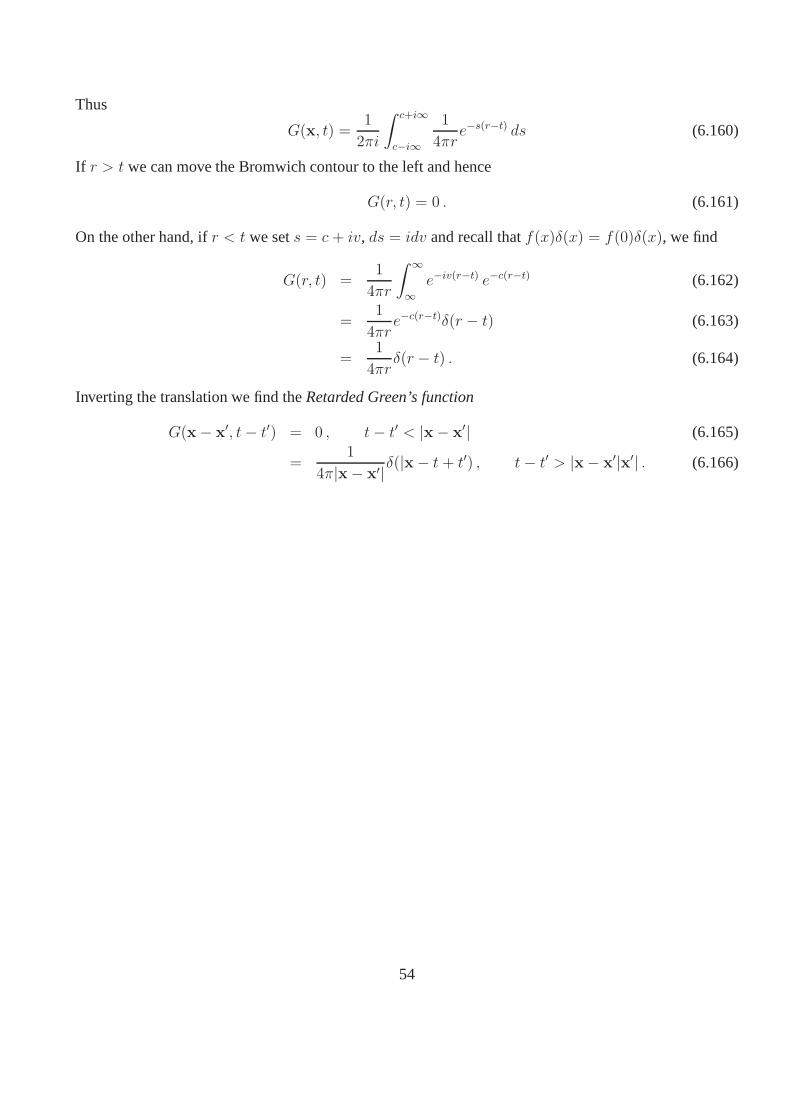
Thus
G(x, t) =1
2πi
∫ c+i∞
c−i∞
1
4πre−s(r−t) ds (6.160)
If r > t we can move the Bromwich contour to the left and hence
G(r, t) = 0 . (6.161)
On the other hand, ifr < t we sets = c + iv, ds = idv and recall thatf(x)δ(x) = f(0)δ(x), we find
G(r, t) =1
4πr
∫ ∞
∞e−iv(r−t) e−c(r−t) (6.162)
=1
4πre−c(r−t)δ(r − t) (6.163)
=1
4πrδ(r − t) . (6.164)
Inverting the translation we find theRetarded Green’s function
G(x − x′, t− t′) = 0 , t− t′ < |x − x′| (6.165)
=1
4π|x − x′|δ(|x − t+ t′) , t− t′ > |x − x′|x′| . (6.166)
54