comparing radial velocities of atmospheric lines with ... · 2012 the authors, mnrasc 420,...

Mon. Not. R. Astron. Soc. 420, 2874–2883 (2012) doi:10.1111/j.1365-2966.2011.20015.x

Comparing radial velocities of atmospheric lines with radiosondemeasurements

P. Figueira,1� F. Kerber,2 A Chacon,3 C. Lovis,4 N. C. Santos,1

G. Lo Curto,2 M. Sarazin2 and F. Pepe4

1Centro de Astrofısica, Universidade do Porto, Rua das Estrelas, 4150-762 Porto, Portugal2European Southern Observatory, Karl-Schwarzschild-Strasse 2, D-85748 Garching bei Munchen, Germany3Departamento de Fısica y Astronomıa, Universidad de Valparaıso, Av. Gran Bretana 1111, Valparaıso, Chile4Observatoire Astronomique de l’Universite de Geneve, 51 Ch. des Maillettes, Sauverny CH1290, Versoix, Switzerland

Accepted 2011 October 14. Received 2011 October 10; in original form 2011 August 29

ABSTRACTThe precision of radial velocity (RV) measurements depends on the precision attained on thewavelength calibration. One of the available options is to use atmospheric lines as a natural,freely available wavelength reference. Figueira et al. measured the RV of O2 lines using HighAccuracy Radial velocity Planet Searcher (HARPS) and showed that the scatter was only of∼10 m s−1 over a time-scale of 6 yr. Using a simple but physically motivated empirical model,they demonstrated a precision of 2 m s−1, roughly twice the average photon noise contribution.In this paper, we take advantage of a unique opportunity to confirm the sensitivity of thetelluric absorption lines’ RV to different atmospheric and observing conditions by means ofcontemporaneous in situ wind measurements. This opportunity is a result of the work doneduring site testing and characterization for the European Extremely Large Telescope (E-ELT).The HARPS spectrograph was used to monitor telluric standards while contemporaneousatmospheric data were collected using radiosondes. We quantitatively compare the informationrecovered by the two independent approaches.

The RV model fitting yielded results similar to that of Figueira et al., with lower windmagnitude values and varied wind direction. The probes confirmed the average low windmagnitude and suggested that the average wind direction is a function of time as well. However,these results are affected by large uncertainty bars that probably result from a complex windstructure as a function of height. The two approaches deliver the same results in what concernswind magnitude and agree on wind direction when fitting is done in segments of a coupleof hours. Statistical tests show that the model provides a good description of the data on alltime-scales, being always preferable to not fitting any atmospheric variation. The smaller thetime-scale on which the fitting can be performed (down to a couple of hours), the better thedescription of the real physical parameters is. We then conclude that the two methods delivercompatible results, down to better than 5 m s−1 and less than twice the estimated photon noisecontribution on O2 lines’ RV measurement. However, we cannot rule out that parameters α

and γ (dependence on airmass and zero-point, respectively) have a dependence on time orexhibit some cross-talk with other parameters, an issue suggested by some of the results.

Key words: atmospheric effects – instrumentation: spectrographs – methods: observational –techniques: radial velocities.

1 IN T RO D U C T I O N

The research on extrasolar planets is currently one of the fastestgrowing fields in astrophysics. Triggered by the pioneering work of

�E-mail: [email protected]

Mayor & Queloz (1995) on 51 Peg, it evolved into a domain of itsown, with more than 500 planets confirmed up to date. Most of theseplanets (∼90 per cent) were detected using the radial velocity (RV)induced on the star by the orbital motion of the planet around it.The measurement of precise RVs can only be done against a precisewavelength reference, and two different approaches were pursuedextensively. The first approach was the usage of a Th–Ar emission

C© 2012 The AuthorsMonthly Notices of the Royal Astronomical Society C© 2012 RAS

Comparing RV with radiosonde data 2875

lamp with the cross-correlation function (CCF) method (Baranneet al. 1996), and the second approach made use of the I2 cell alongwith the deconvolution procedure (Butler et al. 1996). In orderto measure precise RV in the infrared (IR) with CRIRES (Kaeuflet al. 2004), Figueira et al. (2010) recovered a method known fora long time: the usage of atmospheric features as a wavelengthanchor. Using CO2 lines present in the H band, the authors attaineda precision of ∼5 m s−1 over a time-scale of one week. While asimilar precision had been attained in the past in the optical domainusing O2 lines, the studies on the stability of atmospheric lines werelimited to a time-scale of up to a couple of weeks.

In order to assess the RV stability of atmospheric lines over longertime-scales, Figueira et al. (2010) used High Accuracy Radial ve-locity Planet Searcher (HARPS) archival data, spanning more thansix years. Three stars – Tau Ceti, μ Arae and e Eri – were se-lected because they provided a strong luminous background againstwhich the atmospheric lines could be measured, and were observednot only over a long time span but with high temporal frequency(in asteroseismology campaigns). The spectra were cross-correlatedagainst an O2 mask using the HARPS pipeline, which delivered theRV, bisector span (BIS) and associated uncertainties. The high in-trinsic stability of HARPS allowed one to measure these effectsdown to 1 m s−1 of precision, roughly the photon noise attained onthe atmospheric lines.

The rms of the velocities turned out to be only ∼10 m s−1, andyet well in excess of the attained photon noise. An inspection of theRV pattern on one star over one night revealed not white noise buta well-defined shape on RV, BIS, contrast and full width at half-maximum. A component of the RV signal was associated with BISvariation, which in turn was linearly correlated with the airmass atwhich the observation was performed. A second component of thesignal was interpreted as being the translation of the atmosphericlines’ centre created by the projection of an average horizontal windvector along the line of sight. These two effects were described bythe formula

� = α

(1

sin(θ )− 1

)+ β cos(θ ) cos(φ − δ) + γ, (1)

where α is the proportionality constant associated with the variationin airmass, β and δ are the average wind speed magnitude anddirection, and θ and φ are the telescope elevation and azimuth,respectively. γ represents the zero-point of the RV, which can differfrom zero. The fitting of the variables α, β, γ and δ allowed agood description of the telluric RV signal, with the scatter aroundthe fit being around 2 m s−1, or twice the photon noise. The fittingwas performed in two ways: first, allowing all parameters to varyfreely and secondly, imposing the same α and γ for different datasets. For details the interested reader is referred to the originalpaper. However, the model represented by equation (1), while beingphysically motivated, was not fully validated due to the absenceof wind measurements against which the fitted values could becompared.

Precipitable water vapour (PWV), the major contributor to theopacity of Earth’s atmosphere in the IR is among the atmosphericparameters studied during European Extremely Large Telescope(E-ELT) site testing. Hence, the mean PWV established over longtime-scales determines how well a site is suited for IR astronomy.For the E-ELT site characterization a combination of remote sensing(satellite data) and on-site data was used to derive the mean PWVfor several potential sites, taking La Silla and Paranal as reference(Kerber et al. 2010). In order to better understand the systematics inthe archival data and to obtain data at higher time resolution, a total

of three campaigns were conducted at La Silla Paranal observatoryin 2009. During each campaign all available facility instrumentsas well as dedicated IR radiometers were used to measure PWVfrom the ground (Kerber et al., in preparation; Querel, Naylor &Kerber 2011). In addition, radiosondes were launched to measurethe vertical profile of atmospheric parameters in situ, with the goalof calculating the real PWV in the atmosphere. Radiosondes are anestablished standard in atmospheric research and all other methodswere validated with respect to the radiosonde results with very highfidelity (Chacon et al. 2010; Kerber et al. 2010; Querel et al. 2010).

In the current paper, we present the results of exploiting data fromthe above campaigns: since HARPS observations and radiosondemeasurements were made in parallel we are in a position to make adirect and quantitative comparison of the wind speed parameters (βand δ). The paper is structured as follows. In Section 2 we describethe data acquisition and reduction of both observing campaigns.Section 3 is dedicated to the description of the analysis of data andsubsequent results. In Section 4 we discuss the implications of ourresults, and we conclude in Section 5 with the lessons learned fromthis campaign.

2 O B S E RVAT I O N S A N D DATA R E D U C T I O N

2.1 HARPS measurements

HARPS (Mayor et al. 2003) is a high-resolution fibre-fed cross-dispersed echelle spectrograph installed at the 3.6-m telescope atLa Silla Observatory. It is characterized by a spectral resolutionof 110 000 and its 72 orders cover the whole optical range, from380 to 690 nm. Its extremely high stability allows one to measureRV to a precision of better than 60 cm s−1 when a simultaneousTh–Ar lamp is used, and of around 1 m s−1 without the lamp. Adedicated pipeline (nicknamed DRS for Data Reduction Software)was created to allow for on-the-fly data reduction and RV calcula-tion. This pipeline delivers the RV by cross-correlating the obtainedspectra with a weighted binary mask. To calculate the atmosphericlines’ RV variation one needs only to construct a template maskrepresenting the lines to monitor. This weighted binary mask (Pepeet al. 2002) was built using the HITRAN data base (Rothman et al.2005) to select the O2 lines present in the HARPS wavelength do-main. For details on HARPS, the data reduction procedure and themask construction, the reader is referred to Figueira et al. (2010).The procedure is identical, with the exception that the observationsused in the current paper were performed without simultaneousTh–Ar.

For this programme, nine stars were observed: HR3090, HR3476,HR4748, HR5174, HR5987, HR6141, HR6930, HR7830 andHR8431, which are fast-rotating A-B stars, mostly featureless inthe optical domain and suitable to be used as telluric standards. Fordetails on the stars the reader is referred to the website ‘Stars forMeasuring PWV with MIKE’1 and to Thomas-Osip et al. (2007).A total of 1120 measurements were collected on 2009 May 8 and9 during the course of two nights of technical time. The stars wereobserved in a complex pattern in such a way that both low and highairmass and different patches of the sky were probed throughoutthe night in order to sample any variations of PWV. The main con-sequence is that even a fraction of the night with a couple of hourscan contain observations of several stars at a wide range of airmass

1 http://www.lco.cl/operations/gmt-site-testing/stars-for-measuring-pwv-with-mike/stars-for-measuring-pwv

C© 2012 The Authors, MNRAS 420, 2874–2883Monthly Notices of the Royal Astronomical Society C© 2012 RAS

2876 P. Figueira et al.

and elevation/azimuth coordinates, covering well the independentvariables of equation (1) and allowing a precise estimation of theparameters to be fitted.

2.2 Radiosonde measurements

The radiosonde (Vaisala RS-92) is a self-contained instrument pack-age with sensors to measure e.g. temperature and humidity com-bined with a GPS receiver and a radio transmitter that relays alldata in real time to a receiver on the ground. The radiosonde is tiedto a helium-filled balloon and after launch it ascends at a rate of afew m s−1 following the prevailing winds. On its ascent, the sondewill sample the local atmospheric conditions up to an altitude of∼20 km, when the balloon will burst. By that time it travels horizon-tally ∼100 km from the launch site. Since it relays its 3D locationbased on GPS location every 2 s, the wind vector exerting force onthe balloon can be deduced from the change in GPS position.

A total of 17 radiosondes were launched between 2009 May5 and 15 from the La Silla site. One or two launches were con-ducted every day/night. On the 13th no data were collected due toa technical problem when radio contact with the radiosonde waslost shortly after lunch. From the collected physical parameters, thesix of interest for our study, as well as the nominal precision ofthe measurements, are presented in Table 1. As the sondes rise inheight, they measure the two horizontal wind components on eachlayer with a nominal precision of 1 × 10−3 m s−1, much higher thanthat of contemporaneous RV measurements.

Radiosondes form the backbone of the global network coor-dinated by the World Meteorological Organization (WMO) formeasuring conditions at the surface and in Earth’s atmosphere bycombining the in situ atmospheric sounding with measurementstaken onboard ships, aircraft and satellites. Coordinated radiosondelaunches (one launch at 12:00 UTC is the minimum requirement,other launch times are 00, 06 and 18 h UTC) provide a global snap-shot of atmospheric conditions which are then used as basic inputfor describing its current state and for modelling future conditions.

The recommended maximum distance between stations is 250 kmbut the global distribution is very uneven and biased towardsheavily populated areas in the Northern hemisphere. South Amer-ica is sparsely covered with Chile-operating four stations onlyone of which (Santo Domingo, WMO station number 85586)launches two radiosondes per day at 00 and 12 UTC. Data fromall active launch sites can be found at http://weather.uwyo.edu/upperair/sounding.html.

The WMO also defines the requirements in terms of equipmentand procedures such as number of barometric pressure levels, etc.A number of different radiosondes from different manufacturersare used in various countries. To ensure comparability the WMOregularly conducts cross-calibration campaigns with parallel mea-

Table 1. The six parameters used from the data collected by radiosondes.

Parameter Unit Precision (unit) Comment

Time s 0.1 Measurement cadence of one every 2 sT K 0.1 –P hPa 0.1 –Height m 1 Limited to 30 kmu m s−1 0.01 E–W wind component, east positivev m s−1 0.01 N–S wind component, north positive

surements.2 The Vailsala radiosonde RS-92 used in our campaign isconsidered to be the most reliable and accurate commercial deviceavailable. Its minor biases in particular for day-time launches arewell documented (Jauhiainen & Lehmuskero 2005; Miloshevichet al. 2009).

The global snapshot of the state of the atmosphere, taken at 00:00and 12:00 UTC, is used as an initial condition for global meteoro-logical numerical models [GFS (1), ECMWF (2), GME (3) amongothers3].

These initial conditions are employed in numerical approxima-tions using dynamical equations, which predict the future state ofthe atmospheric circulation (Holton 2005). The models are a simpli-fication of the atmosphere because the horizontal resolution of thegrid can be between 60 km (GME) and 100 km (GFS) – and some-times more – and the vertical resolution provides only very smallnumber of layers, but on a global scale the results are very good andhave improved considerably over the past decades. There are othermodels called mesoscale models [MM5 (4), WRF (5), MesoNH (6),among others], which provide higher spatial resolution (horizontaland vertical) and use more specific dynamical equations (physicsparametrization) and better resolution of the surface terrain. Theinitial conditions for these models are usually the global modelaugmented by some local weather stations. Details on the modelsare available from the sites mentioned above.

Concerning the applicability of RS data for our purpose it is im-portant to note that the radiosonde is the accepted standard in atmo-spheric and meteorological research. For global weather forecastinga distance of the order of 250 km between the radiosonde launchstations is the desired distance but by no means is this standardachieved always, while the cadence is between 6 and 24 h. Hence,the radiosonde data set that we use for comparison with HARPSobservations is well within the accepted limits of applicability interms of spatial and time resolution.

It is evident that local topography and diurnal variations maylimit the value of a set of radiosonde data to smaller distancesand shorter periods of time. To this end there is a very instruc-tive analysis by Kalthoff et al. (2002), which is directly applica-ble to our case. They use the Karlsruhe atmospheric mesoscalemodel (KAMM) and compare with wind measurements taken atstations around 30◦ south in Chile, including the Cerro Tololo Inter-American Observatory (CTIO). La Silla (70◦44′4.′′5 W 29◦15′15.′′4S) is located within that region only about 100 km north of CTIO.Kalthoff et al. (2002) find that the wind patterns over this region

2 Performance of the Vaisala Radiosonde RS-92-SGP and Vaisala Digi-CORA Sounding System MW31 in the WMO Mauritius RadiosondeIntercomparison, 2005 February. Webpage http://www.vaisala.com/Vaisala%20Documents/White%20Papers/Vaisala%20Radiosonde%20RS92%20in%20Mauritius%20Intercomparison.pdf.3 (1) Global Forecast System (http://www.emc.ncep.noaa.gov/gmb/moorthi/gam.html).(2) European Center of Medium range Weather Forecasting (http://www.ecmwf.int/products/data/operational_system/description/brief_history.html).(3) Global Numerical Weather Prediction Model (http://journals.ametsoc.org/doi/abs/10.1175/1520-0493(2002) 130%3C0319%3ATOGIHG%3E2.0.CO%3B2).(4) The Fifth-Generation NCAR/Penn State Mesoscale Model. NCAR: Na-tional Center of Atmospheric Research (http://www.mmm.ucar.edu/mm5/).(5) Weather Research and Forecasting model (http://www.wrf-model.org/index.php).(6) Non-Hydrostatic Mesoscale Atmospheric Model (http://mesonh.aero.obs-mip.fr/mesonh/).



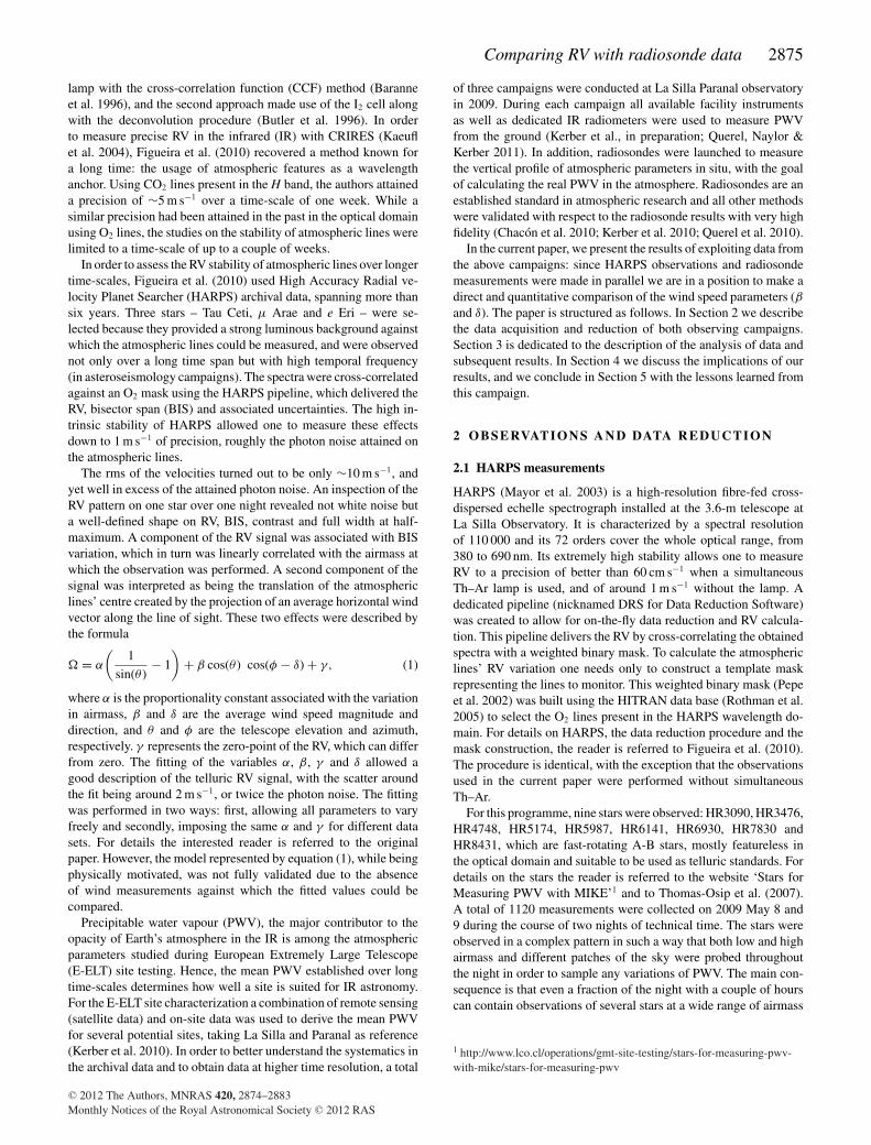
Table 2. The fitted parameters and data properties, before and after the fitted model is subtracted from it, with all parameters kept varying freely (top), andwhen α and β are imposed as the same for the data sets (bottom, marked with *).

Data set No. of observations σ (m s−1) σ(O−C) (m s−1) σph (m s−1) χ2red α (m s−1) β (m s−1) γ (m s−1) δ (◦)

08+09-05-2009 1093 5.01 4.14 2.82 2.20 7.79+0.76−0.73 8.47+0.76

−0.68 220.56+0.05−0.31 126.10+4.41

−5.56

08-05-2009 (1st n.) 554 5.36 4.38 2.92 2.12 5.74+1.87−1.81 13.93+3.12

−2.61 220.32+0.31−0.79 145.14+5.58

−13.00

09-05-2009 (2nd n.) 539 4.60 3.68 2.72 1.83 8.20+0.83−0.81 6.75+0.60

−0.50 219.95+0.36−0.04 97.75+6.67

−7.91

(1st n., section 1/3) 185 3.46 2.89 1.88 2.25 8.97+1.41−1.41 4.44+3.31

−0.89 223.58+0.97−0.75 42.17+47.29

−17.60

(1st n., section 2/3) 185 4.58 4.58 3.27 1.71 10.79+21.27−17.98 15.99+43.88

−8.00 223.96+5.24−4.91 17.22+77.04

−96.66

(1st n., section 3/3) 184 6.26 4.51 3.60 1.53 29.77+11.86−12.13 74.86+41.90

−31.07 230.09+5.25−5.30 4.28+63.12

−2.35

(2nd n., section 1/3) 180 4.80 3.30 2.52 1.73 15.50+1.70−1.71 15.98+4.50

−3.19 223.51+1.28−1.18 24.96+18.08

−7.08

(2nd n., section 2/3) 180 4.50 3.74 2.84 1.75 8.76+2.47−2.38 3.61+5.17

−0.78 220.10+0.91−0.50 90.87+31.05

−47.05

(2nd n., section 3/3) 180 3.86 3.48 2.82 1.58 −15.06+18.00−18.04 7.78+2.77

−1.77 220.61+0.74−0.70 66.26+17.98

−27.05

08-05-2009 (1st n.)* 554 5.36 4.38 2.92 2.12† 6.85 +0.76−0.77 13.57 +1.31

−1.25 220.19 +0.13−0.23 143.17 +2.94

−3.72

09-05-2009 (2nd n.)* 539 4.60 3.68 2.72 1.83† 6.85 +0.76−0.77 6.95 +0.69

−0.60 220.19 +0.13−0.23 102.14 +6.81

−8.25Global fitting parameters 1093 5.01 4.06 2.82 1.98 – – – –

(1st n., section 1/3)* 185 3.46 2.97 1.88 2.34† 8.81 +1.09−1.09 6.05 +2.00

−1.41 221.39 +0.42−0.39 127.53 +10.59

−23.16

(1st n., section 2/3)* 185 4.58 4.62 3.27 1.73† 8.81 +1.09−1.09 14.38 +8.65

−4.70 221.39 +0.42−0.39 131.27 +7.37

−53.92

(1st n., section 3/3)* 184 6.26 4.55 3.60 1.55† 8.81 +1.09−1.09 11.17 +1.44

−0.55 221.39 +0.42−0.39 77.45 +16.67

−15.42

(2nd n., section 1/3)* 180 4.80 3.49 2.52 1.90† 8.81 +1.09−1.09 8.00 +1.01

−0.73 221.39 +0.42−0.39 71.89 +14.36

−13.51

(2nd n., section 2/3)* 180 4.50 3.78 2.84 1.78† 8.81 +1.09−1.09 9.23 +4.15

−2.92 221.39 +0.42−0.39 5.39 +36.17

−7.01

(2nd n., section 3/3)* 180 3.86 3.53 2.82 1.62† 8.81 +1.09−1.09 13.47 +1.82

−1.59 221.39 +0.42−0.39 95.93 +8.41

−9.63

Global fitting parameters 1093 5.01 3.87 2.82 1.81 – – – –

Note that δ = 0◦ when wind direction points towards north and positive eastwards. The error bars on each of the fitted parameters were drawn by bootstrappingthe residuals (see text for details). Note that the χ2

red marked with † are not defined in the strict sense: they are calculated assuming four fitting parameters forthe considered subset, with the objective of allowing comparison with the corresponding unconstrained fitting.

are stable, their diurnal variations are highly reproducible and thatwind conditions are mostly stable during night time. Their mainfinding is that for altitudes between 2 and 4 km northerly windsprevail whereas above 4 km large-scale westerly winds dominate.The reason for the northerly wind is a deflection of westerly windsby the Cordillera de los Andes which forms a barrier. They pro-vide a physical explanation (their Section 4) in terms of the Froudenumber (ratio between inertial forces and buoyancy) demonstratingthat this deflected northerly flow is a naturally stable phenomenon.As mentioned La Silla is located in the same region and the windroses of Cerro Tololo (2200 m) (their fig. 7) and La Silla (2400 m)4

are very similar, clearly showing a predominance of the northerlywind.

In particular, winter months (June–August) are characterized byvery constant daily ground wind properties (fig. 5 of the samepaper). Our observations were made in May. In addition it is a well-established fact that wind conditions in the free atmosphere aremuch more stable than in the turbulent and highly variable groundlayer (see e.g. Holton 2005; Wallace & Hobbs 2006).

As a consequence of the very homogeneous overall wind structurebetween 2 and 4 km and above 4 km we have reason to believe thatthe information on the wind vectors obtained by a radiosonde willbe representative of conditions over the time span of at least a goodfraction of a night for our campaigns.

4 http://www.eso.org/gen-fac/pubs/astclim/lasilla/humidity/LSO \ _meteo_stat-2002-2006.pdf

3 A NA LY SI S AND RESULTS

3.1 HARPS measurements

We analysed the data from the nine stars as if coming from a singledata set, as there is no reason to treat them separately. As done inFigueira et al. (2010), we discarded the 27 data points with photonnoise precision worse than 5 m s−1, which correspond to only 2.5per cent of the observations.

The total RV scatter and average photon noise were 5.01 and2.82 m s−1, respectively. If one separates the set into the two nightsthat constitute it, the values for the first night are 5.36 and 2.92 m s−1,and that for the second night are 4.60 and 2.72 m s−1. We notethat the photon noise contribution to the precision from the stellarspectrum is larger than 1 m s−1, validating the choice of not usingthe lamp simultaneously with observations.

We fitted the RV variation on the two nights using equation (1),as described in Figueira et al. (2010). When fitting, we consideredsplitting the data set in three different ways and making two dif-ferent hypotheses for the parameter variation. On the splitting ofthe data set we employed (1) the same parameters for all the ob-servations, (2) an independent set of parameters per night and (3)a set of parameters for each one-third of the night. After allowingall parameters to vary freely at first, we repeated this imposing α

and γ to be the same for the whole data set in (2) and (3). Theresulting parameters, χ2

red, and scatter around the fit are presented inTable 2 for each case. The error bars were estimated by bootstrap-ping the residuals and repeating the fitting 10 000 times. The 95 percent confidence intervals were drawn from the distribution of theparameters, and the 1σ uncertainty estimations are presented.



Table 3. The probability that the residuals and original data setsare drawn from Gaussian distributions, as estimated by using theKolmogorov–Smirnov test (see text for details). We represent byPKS the fit in which the parameters can vary freely and by PKS(constfit) the fit in which α and β are imposed to be the same.

Data set PKS PKS(const fit) PKS(no fit)

08+09-05-2009 1.47e−12 – 4.32e−2508-05-2009 (1st n.) 2.10e−06 8.62e−06 6.28e−1909-05-2009 (2nd n.) 9.29e−05 4.44e−04 2.62e−10(1st n., section 1/3) 1.36e−01 4.01e−03 1.22e−05(1st n., section 2/3) 4.68e−02 5.06e−02 3.02e−02(1st n., section 3/3) 1.46e−01 4.22e−02 1.07e−05(2nd n., section 1/3) 1.81e−01 3.31e−02 5.79e−08(2nd n., section 2/3) 1.22e−01 3.41e−01 4.66e−03(2nd n., section 3/3) 1.84e−01 7.93e−02 5.33e−02

While one might be tempted to compare the χ2red of the data as a

way of quantifying the quality of the fit, there are several reasons notto do so. The first is that as one divides the data into subsets that arefitted independently, there is some ambiguity in how the χ2

red of a setis compared with the combined χ2

red of the subsets. However, moreimportant is that we are considering a problem with priors, as thereader will realize when noting that β ∈ [0, ∞[. The consequence isthat this corresponds to the fitting of a non-linear model, for whichthe number of degrees of freedom is ill-defined, as recently under-lined by Andrae, Schulze-Hartung & Melchior (2010). In order tocompare the quality of the data represented by the different models,we follow the recommendations of the same authors. We calculatethe probability that the normalized residuals of the fit are drawnfrom a Gaussian distribution with μ = 0 and σ = 1, as expectedif no signal is present and the scatter is dominated by the measure-ment uncertainty. To do so we use the Kolmogorov–Smirnov test(as implemented in Press et al. 1992) and compute the probabilityPKS which, loosely speaking, corresponds to the probability that theresiduals after fitting the model are drawn from a Gaussian distri-bution. The larger the value of PKS, the more appropriate the modelis to describe the data set in hands. We also calculated the proba-bility PKS(nofit) for normalized RVs of each data set without fittingthe model, but from which only the average value was subtracted(which corresponds to fitting only a constant). The probability foreach case on each data set is presented in Table 3.

3.2 Radiosonde measurements

The measurement of the radiosonde wind vector (u, v) as a functionof time or height, while interesting, is hardly insightful for ourobjective. We need to calculate the effect of this wind as integratedalong the line of sight, such as when it is measured by any telescopeand spectrograph on the ground. This will deliver an average windvector which can then be compared with the one obtained withHARPS (see the previous section).

A way of calculating this average wind is to consider a plane-parallel atmosphere that is composed of horizontal layers. Everyradiosonde measurement probes the properties of a layer in its as-cent. To obtain the average wind speed we weight the wind speedof each of these layers with its absorptivity. In doing so, we are con-sidering that the absorption line we measure with our spectrographis the result of the product of the transmission of all layers, and eachone of these creates a small line shifted by its respective horizontalwind. It is important to note that we do this because absorptivityis proportional to the depth of the line at the central wavelength,

and thus proportional to the spectral information contribution forthe CCF as described in Pepe et al. (2002).

The absorptivity on each layer is Ai = 1 − e−τ where τ is theoptical depth and is calculated as τ = I (T ) × AmplitudeLorentz ×σO2 (T , P ) h where I is the spectral line intensity, AmplitudeLorentz

is the relative amplitude of a Lorentzian function, σO2 is the surfacedensity of O2 and h is the height of the layer in question.

The first component of τ is I, the spectral line intensity (basi-cally the line area), and is given in [cm−1 (molecule cm−2)−1] inHITRAN. Since I is a function of T we calculated a grid of HI-TRAN I from the minimum to the maximum temperature measuredby the radiosondes, with a step of 0.1 K for all the O2 lines withinHARPS wavelength domain. For each temperature an average I wasassigned to the overall spectrum. This gives us I(T), and to obtainvalues for T in between two grid points we fitted second-degreepolynomials, which provided a very smooth description of the data.Interpolating the values provided the same wind values down to0.01 m s−1.

In order to derive the line depth, one has to apply a correction toget the amplitude of the Lorentzian function that has the equivalentarea given by 1.0/(π×HWHM), in which HWHM is the half-widthat half-maximum. The HWHM was set to 1.0, but its absolute valuedoes not affect the results significantly, for it affects all layers inthe same way. Subsequent tests showed that changing it from 0.1to 10 led to variations of the order of 0.01 m s−1 and 0.◦01 on windmagnitude and direction, much smaller than the error bars of themeasurements. The surface density σO2 (T , P ) was calculated usingthe ideal gas law and assuming a constant volume mixing ratio ofO2 of 20.946 per cent as a function of height, which is a reasonableassumption up to 80 km, and hence well justified in the range ofinterest of up to 30 km.

With this we calculated the weighted average of the velocities aswell as a weighted standard deviation. The error on the average isestimated to be the weighted standard deviation. To allow compari-son with the results from the previous section, one can calculate thevector magnitude and direction. The results are presented in Table 4and plotted in Fig. 1.

4 D I SCUSSI ON

4.1 The RV data

The first point to note when it comes to the results of Table 2is the low value of the rms of RVs over the two nights: 5 m s−1,which is less than twice the average photon noise value. As oneselects smaller sets of data, first individual nights and then subsetsof these nights, one obtains different fit parameters. This suggeststhat the parameters are variable on a time-scale smaller than onenight. The higher probability PKS presented by the short-time-scaledata sets attests to the fact that the model is more suitable to test thevariability on smaller time-scales. The fitting performed imposingthe same α and γ provides results with similar quality, better forthe complete nights fitting, poorer if the nights are divided intosubsections. Moreover, when comparing the fitted data with the rawdata, one concludes that fitting the data with the models leads toresiduals that are closer to Gaussian than subtracting a constant fromit. This means that the model description, even when less precise,still describes a fraction of the signal contained in the data and isalways preferable over using raw data.

It is insightful to compare the data with that of Figueira et al.(2010). The fitted α and β are comparable, and tend to be evenlower, while γ is similar in value. Importantly, δ varies significantly



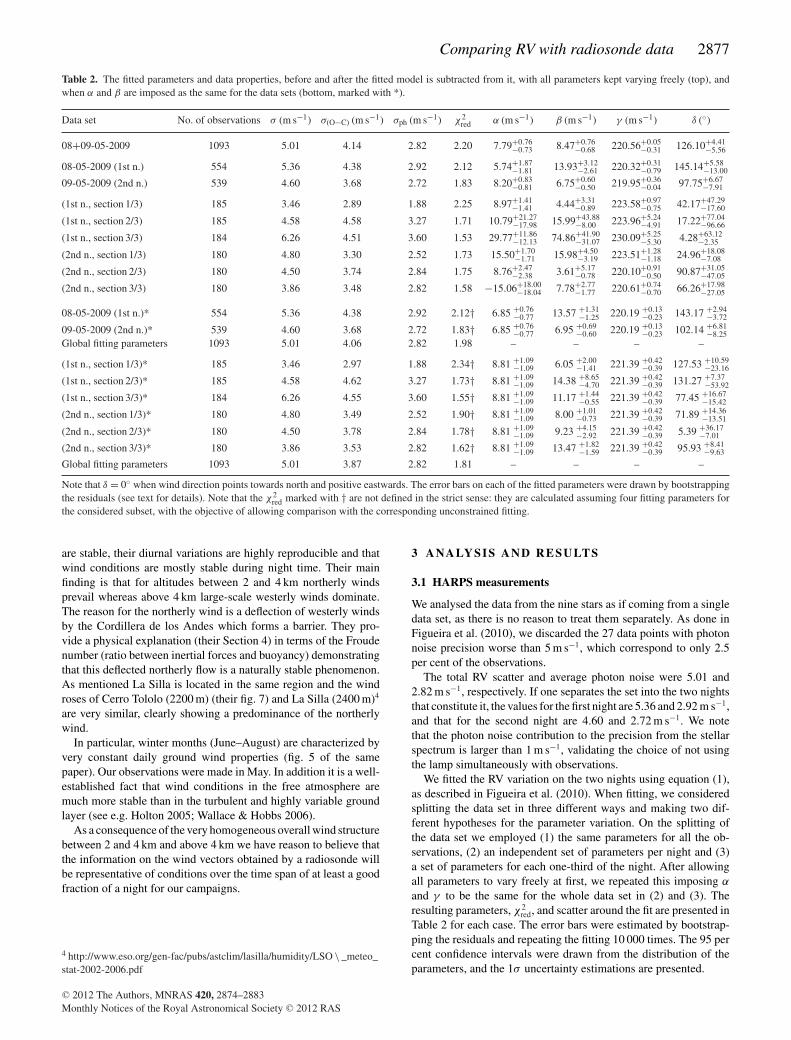
Table 4. Weighted average of wind components u and v, as well as wind vector magnitude and direction for each ofthe radiosondes launched.

Probe no. Observation date and hour u (m s−1) v (m s−1) ‖u + v‖ (m s−1) δ (◦)

1 EDT/05/05/09/1200 UTC −9.43 ± 5.71 7.91 ± 10.95 12.31 ± 8.28 −50.01 ± 42.622 EDT/06/05/09/1200 UTC −11.10 ± 5.92 5.48 ± 8.05 12.38 ± 6.39 −63.71 ± 35.543 EDT/07/05/09/0600 UTC −9.00 ± 7.53 2.40 ± 7.30 9.31 ± 7.52 −75.07 ± 45.004 EDT/08/05/09/0000 UTC 3.44 ± 8.55 4.09 ± 10.27 5.35 ± 9.60 40.03 ± 99.695 EDT/08/05/09/0600 UTC −0.58 ± 7.76 7.22 ± 9.54 7.25 ± 9.53 −4.58 ± 61.426 EDT/09/05/09/0000 UTC −3.43 ± 6.96 8.61 ± 8.40 9.27 ± 8.22 −21.70 ± 44.497 EDT/09/05/09/0600 UTC −2.50 ± 7.46 10.85 ± 8.55 11.13 ± 8.50 −12.97 ± 38.698 EDT/09/05/09/1200 UTC −3.34 ± 4.82 16.05 ± 11.78 16.40 ± 11.57 −11.75 ± 18.499 EDT/10/05/09/0000 UTC 5.16 ± 8.98 9.81 ± 9.48 11.09 ± 9.37 27.74 ± 46.9910 EDT/10/05/09/ 0600 UTC 3.12 ± 6.95 7.88 ± 7.33 8.48 ± 7.28 21.58 ± 47.3111 EDT/ 11/05/09/0000 UTC 3.24 ± 3.54 10.67 ± 7.00 11.15 ± 6.78 16.89 ± 20.3012 EDT/11/05/09/0600 UTC 2.76 ± 3.34 10.20 ± 6.31 10.57 ± 6.16 15.14 ± 19.6313 EDT/12/05/09/0000 UTC 3.63 ± 3.46 11.27 ± 6.62 11.84 ± 6.39 17.83 ± 18.7014 EDT/14/05/09/0000 UTC 14.69 ± 10.42 12.54 ± 7.69 19.31 ± 9.37 49.53 ± 26.5215 EDT/14/05/09/1200 UTC 11.00 ± 7.69 8.09 ± 5.96 13.66 ± 7.13 53.69 ± 27.7716 EDT/15/05/09/0000 UTC 10.66 ± 8.44 6.66 ± 4.69 12.57 ± 7.57 57.98 ± 27.2717 EDT/15/05/09/0600 UTC 10.32 ± 8.41 8.84 ± 6.49 13.59 ± 7.66 49.43 ± 31.05

Note that δ = 0◦ when wind direction points towards north and positive eastwards.

Figure 1. Evolution of average wind magnitude ( upper panel) and direction(lower panel), as measured by the radiosondes. The two nights during whichobservations with HARPS were performed are represented by shadowedand coloured zones. The values are presented in Table 4.

from one data set to the other, just as it varied between the data setsconsidered in the previous paper. It is important to note that the errorbars on some measurements are rather large, and the discrepancybetween some consecutive measurements can be explained by thisalone. In particular, the last two-thirds of the first night were affectedby a high photon noise contribution, and these two sets yield thefits with the largest and more asymmetric error bars and largestresiduals for the unconstrained fit. However, the scatter is alreadysmaller than twice the photon noise, with or without subtracting thefit.

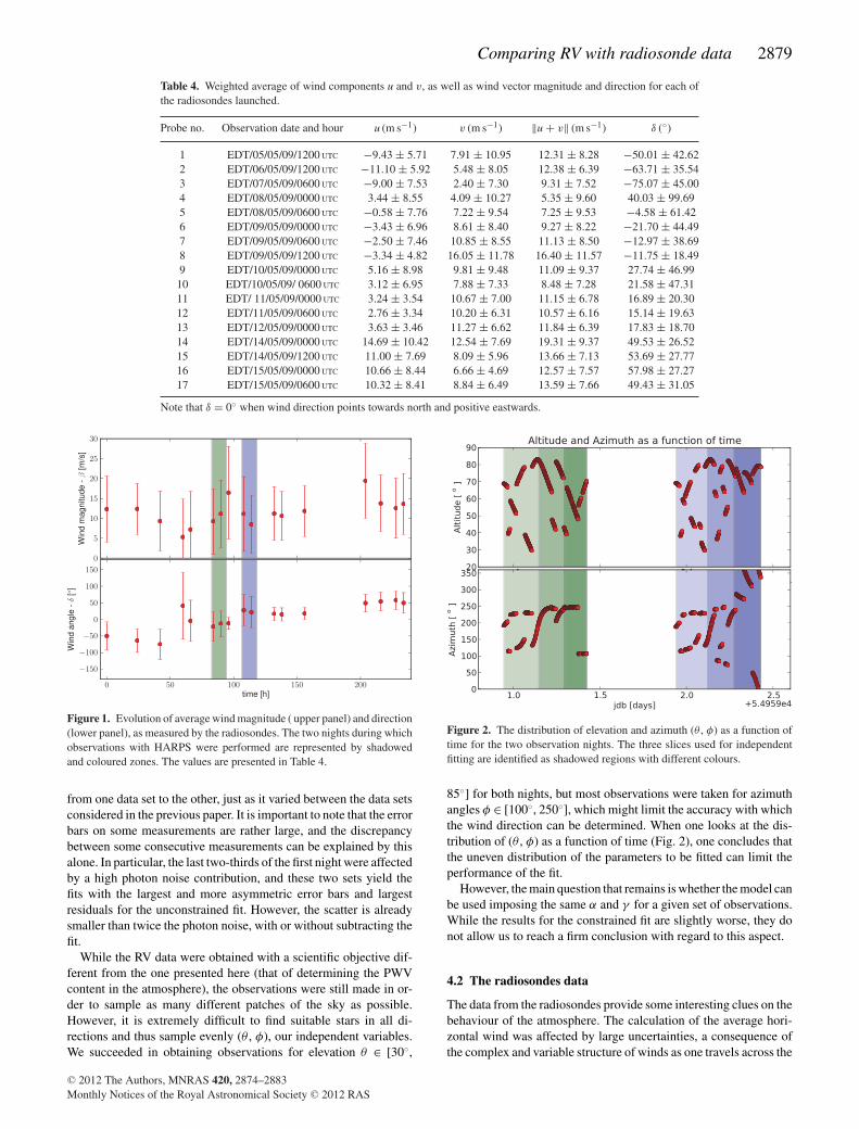
While the RV data were obtained with a scientific objective dif-ferent from the one presented here (that of determining the PWVcontent in the atmosphere), the observations were still made in or-der to sample as many different patches of the sky as possible.However, it is extremely difficult to find suitable stars in all di-rections and thus sample evenly (θ , φ), our independent variables.We succeeded in obtaining observations for elevation θ ∈ [30◦,

Figure 2. The distribution of elevation and azimuth (θ , φ) as a function oftime for the two observation nights. The three slices used for independentfitting are identified as shadowed regions with different colours.

85◦] for both nights, but most observations were taken for azimuthangles φ ∈ [100◦, 250◦], which might limit the accuracy with whichthe wind direction can be determined. When one looks at the dis-tribution of (θ , φ) as a function of time (Fig. 2), one concludes thatthe uneven distribution of the parameters to be fitted can limit theperformance of the fit.

However, the main question that remains is whether the model canbe used imposing the same α and γ for a given set of observations.While the results for the constrained fit are slightly worse, they donot allow us to reach a firm conclusion with regard to this aspect.

4.2 The radiosondes data

The data from the radiosondes provide some interesting clues on thebehaviour of the atmosphere. The calculation of the average hori-zontal wind was affected by large uncertainties, a consequence ofthe complex and variable structure of winds as one travels across the



Table 5. Weighted average of wind components u and v, as well as wind vector magnitude and direction for each of theradiosondes launched.

Data set β (m s−1) δ (◦) # Probe (Time distance) ‖u + v‖ (m s−1) δ (◦)

08+2009-05-09 8.47+0.76−0.68 126.10+4.41

−5.56 8 (4 h) 16.40 ± 11.57 −11.75 ± 18.49

2009-05-08 (1st n.) 13.93+3.12−2.61 145.14+5.58

−13.00 7 (1 h) 11.13 ± 8.50 −12.97 ± 38.69

09-05-2009 (2nd n.) 6.75+0.60−0.50 97.75+6.67

−7.91 10 (1.5 h) 8.48 ± 7.28 21.58 ± 47.31

(1st n., section 1/3) 4.44+3.31−0.89 42.17+47.29

−17.60 6 (1.5 h) 9.27 ± 8.22 −21.70 ± 44.49

(1st n., section 2/3) 15.99+43.88−8.00 17.22+77.04

−96.66 7 (0.5 h) 11.13 ± 8.50 −12.97 ± 38.69

(1st n., section 3/3) 74.86+41.90−31.07 4.28+63.12

−2.35 7 (2.5 h) 11.13 ± 8.50 −12.97 ± 38.69

(2nd n., section 1/3) 15.98+4.50−3.19 24.96+18.08

−7.08 9 (1 h) 11.09 ± 9.37 27.74 ± 46.99

(2nd n., section 2/3) 3.61+5.17−0.78 90.87+31.05

−47.05 10 (1 h) 8.48 ± 7.28 21.58 ± 47.31

(2nd n., section 3/3) 7.78+2.77−1.77 66.26+17.98

−27.05 10 (2 h) 8.48 ± 7.28 21.58 ± 47.31

Note that δ = 0◦ when wind direction points towards north and positive eastwards.

atmosphere. However, the average wind magnitude is remarkablylow, being between 5 and 16 m s−1. The values close in time are inagreement within error bars, both in what concerns magnitude anddirection. Note, in particular, the values obtained using probes 6, 7and 8, released 6 h apart and perfectly compatible within their as-signed uncertainty. It is interesting to point out that the measurementyielding the largest uncertainty on wind direction is the one withthe smallest wind magnitude value, as expected. The wind directionmeasurements also suggest a slow variation of wind direction as afunction of time.

4.3 Comparing RV and radiosondes data

In order to compare the two data sets we computed the time centre ofthe observations for each block and selected the probe measurementthat was closest in time to it. Table 5 displays the data in a way thatallows an easy comparison of the average wind vector magnitudeand direction, and the difference between the quantities obtainedwith the two different methods is presented in Fig. 3. We consideredthe unconstrained fit values for this purpose as they show higherPKS. In what concerns wind magnitude the values from the probes

Figure 3. Difference between the average wind magnitude (upper panel)and direction (lower panel) as measured by the two different methods. Thevalues are presented in Table 5. The full data set fit values are coded in red,those corresponding to single-night sets are coded in green and the nightsubdivisions are coded in blue (electronic version only).

agree with the fitted values from RV data for all data sets. The onlyoutlier is the third section of the first night, which presents a verylarge value of β and strongly asymmetric error bars. As discussedearlier, the corresponding HARPS data set has the largest photonnoise contribution, and very poor azimuth coverage (as can be seenin Fig. 2) which can explain the lower quality of the fit. In termsof wind direction, the values concerning the fit of a subsection ofthe night agree with those derived from radiosonde measurements,while those on a longer time-scale do not. The most straightforwardinterpretation is that the constant horizontal wind hypothesis doesnot hold for large time-scales. This is not surprising since windvectors are variable over time. In other words, the fit provides abetter description of the data than no fit, and the residuals are closerto Gaussianity than the raw data, as seen, but the direction hasno physical correspondence. However, as stated before, one has tonote that the σ and σ(O−C) values are already quite close to the σph

level, and that the ratio between any of the former and the latter issmaller than 2. Such ratio values are smaller than those obtained inFigueira et al. (2010), and we cannot discard the fact that we mightbe approaching the limit of extractable information from the currentdata set.

It is arguable that the model might be oversimplistic, and thesmall number of parameters and observables might fundamentallylimit the RV signal it can reproduce. Some results hint that themodel might be incomplete, and we followed these to propose andtest alternative models. However, no improvements were verifiedrelative to the basic model presented earlier. We present the resultsof this rather more exploratory digression in Appendix A.

Perfect agreement between the HARPS observations and the ra-diosonde data cannot be expected for a number of reasons listedbelow. The HARPS spectrum samples a pencil beam through theatmosphere when the star is being tracked, while the radiosondeperforms in situ measurements along its trajectory governed by theprevailing winds. Another drawback is that the atmosphere is onlysampled up to an altitude of 20 km; however, at this altitude thedensity of O2 is 10 times lower than that at the top of a mountain, sothe weight Ai is 10 times smaller. Finally, the radiosonde is expectedto oscillate like a pendulum in its ascent, introducing a signal in themeasured RV which is not rooted in the wind vector it is intendedto probe. In spite of all these limitations, the two data sets agree andprovide a coherent picture of the atmospheric impact on RV varia-tion, down to better than 5 m s−1 and less than twice the estimatedphoton noise contribution on O2 lines’ RV measurement.

A quantitative assessment of the stability of atmospheric absorp-tion lines as presented here is of very practical value for astronomy.



Telluric absorption features are imprinted on observations with as-tronomical spectrographs over a wide wavelength range, particu-larly in the IR. On one hand, this constitutes a complication sincethe features overlay the spectrum of the astronomical target leadingto blends and line shifts. Hence, all observations aiming at a highspectral fidelity in certain regions of the IR need to correct for at-mospheric transmission (e.g. Blake, Charbonneau & White 2010;Seifahrt et al. 2010; Muirhead et al. 2011), and not only necessarilyin the context of RV measurements (e.g. Uttenthaler et al. 2010).With a comprehensive characterization of the atmospheric stability,one can assess for the first time the impact of considering atmo-spheric lines to be at rest or characterized by a constant speed overa given period of time. Their stability (or lack thereof) can explain afraction of the residuals obtained today when fitting the atmospherictransmission with a forward model that yields residuals around afew per cent. On the other hand, the telluric features are also used forwavelength calibration again in particular in the IR where technicalcalibration sources are less common. For physical reasons atomicspectra emitted by lamps show fewer lines and a more uneven dis-tribution than in the optical. The Th–Ar hollow cathode lamp isthe only source whose spectrum has been fully characterized in theIR (Kerber, Nave & Sansonetti 2008), and which is being used onCRIRES, but there are limitations in line density and wavelengthcoverage. Gas cells usually also cover only a limited wavelengthrange. As a result telluric absorption lines are an attractive alter-native in parts of the IR. Based on the results presented here thestability of the atmosphere will easily support the low- and medium-resolution spectroscopy, while in particular for high-resolution andhigh-precision work one has to be cautious. The actual wind veloc-ity vector, and its variation, during the astronomical observationsof course remains unknown without independent measurements.Hence, it is not possible to derive proper error bars for a quantita-tive analysis down to the m s−1 level unless a full analysis followingthe method described in Figueira et al. (2010) is performed.

5 C O N C L U S I O N S

We used HARPS to monitor the RV variation of O2 lines in theoptical wavelength domain. We compared the fitting of a modelas described in Figueira et al. (2010) and the obtained parameterswith those delivered by contemporaneous radiosondes. The two ap-proaches deliver the same results in what concerns wind magnitudeand agree on wind direction when fitting is done in segments of acouple of hours. The large uncertainty bars on the values obtainedfrom radiosondes are likely to be a consequence of a complex windstructure as a function of height, a fact that weakens the applicabilityof the assumption of a strong horizontal wind. We cannot concludewhether the α and γ parameters should be constant as a functionof time or not, or whether a cross-term between them should be in-cluded. However, when these are fixed the wind direction does notagree with that extracted from the radiosonde, which suggests thatthe model might be incomplete at this level. We tested two differentalternative models that tried to address this possible incompletenessof the physical description, but the results were poorer than withthe base model.

Statistical tests showed that the base model provides a gooddescription of the data on all time-scales, being always preferableto not fitting any atmospheric variation, and that smaller the time-scale on which it can be performed (down to a couple of hours),the better the description of the real physical parameters is. It isimportant to note that it is for the data sets with higher PKS thatthe wind parameters derived from RV are compatible with those

extracted from radiosonde measurement. Thus, even though themodel presented in Figueira et al. (2010) can probably still berefined, the agreement is proven down to better than 5 m s−1 andless than twice the estimated photon noise contribution on O2 lines’RV measurement.

AC K N OW L E D G M E N T S

This work was supported by the European Research Coun-cil/European Community under the FP7 through starting grantagreement number 239953, as well as by Fundacao para a Cienciae a Tecnologia (FCT) in the form of grant reference PTDC/CTE-AST/098528/2008. NCS would further like to thank FCT throughprogramme Ciencia 2007 funded by FCT/MCTES (Portugal) andPOPH/FSE (EC).

This work has been funded by the E-ELT project in the context ofsite characterization. The measurements have been made possibleby the coordinated effort of the PWV project team and the obser-vatory site hosting it. We would like to thank all the technical staff,astronomers and telescope operators at La Silla who have helpedus in setting up equipment, operating instruments and supportingparallel observations. We thank the directors of La Silla Paranalobservatory (A. Kaufer, M. Sterzik and U. Weilenmann) for accom-modating such a demanding project in the operational environmentof the observatory and for granting technical time. We particularlythank the ESO chief representative in Chile, M. Tarenghi, for hissupport. It is a pleasure to thank the Chilean Director General deAeronautica Civil (in particular J. Sanchez) for the helpful collabo-ration and for reserving airspace around the observatories to ensurea safe environment for launches of radiosonde balloons. Specialthanks to the members of the Astrometeorological Group at theUniversidad de Valparaiso who supported the radiosonde launches.

R E F E R E N C E S

Andrae R., Schulze-Hartung T., Melchior P., 2010, preprint(arXiv:1012.3754)

Baranne A. et al., 1996, A&AS, 119, 373Blake C. H., Charbonneau D., White R. J., 2010, ApJ, 723, 684Butler R. P., Marcy G. W., Williams E., McCarthy C., Dosanjh P., Vogt S.

S., 1996, PASP, 108, 500Chacon A. et al., 2010, in Stepp L. M., Gilmozzi R., Hall H. J., eds,

Proc. SPIE Vol. 7733, Ground-based and Airborne Telescopes III. SPIE,Belligham, 77334K

Figueira P., Pepe F., Lovis C., Mayor M., 2010, A&A, 515, A106Figueira P. et al., 2010, A&A, 511, A55Holton J., 2005, An Introduction to Dynamic Meteorology. Academic Press,

San Diego, CAKaeufl H.-U. et al., 2004, in Moorwood A. F. M., Iye M., eds, Proc. SPIE

Vol. 5492, Ground-based Instrumentation for Astronomy, SPIE,Bellingham, p. 1218

Kalthoff N. et al., 2002, J. Applied Meteorol., 41, 953Kerber F., Nave G., Sansonetti C. J., 2008, ApJS, 178, 374Kerber F. et al., 2010, in Stepp L. M., Gilmozzi R., Hall H. J., eds, Proc.

SPIE Vol. 7733, Ground-based and Airborne Telescopes III. SPIE,Bellingham, 77331M

Mayor M. et al., 2003, Messenger, 114, 20Mayor M., Queloz D., 1995, Nat, 378, 355Miloshevich L. M., Vomel H., Whiteman D. N., LeBlanc T., 2009, J.

Geophys. Res., 114, D11305Muirhead P. S. et al., 2011, PASP, 123, 709Pepe F., Mayor M., Galland F., Naef D., Queloz D., Santos N. C., Udry S.,

Burnet M., 2002, A&A, 388, 632



Press W. H., Teukolsky S. A., Vetterling W. T., Flannery B. P., 1992, Numer-ical Recipes in FORTRAN. The Art of Scientific Computing. CambridgeUniv. Press, Cambridge

Querel R. R. et al., 2010, in Stepp L. M., Gilmozzi R., Hall H. J., eds,Proc. SPIE Vol. 7733, Ground-based and Airborne Telescopes III. SPIE,Belligham, 773349

Querel R. R., Naylor D. A., Kerber F., 2011, PASP, 123, 222Rothman L. S. et al., 2005, J. Quant. Spectros. Radiative Transfer, 96, 139Seifahrt A., Kaufl H. U., Zangl G., Bean J. L., Richter M. J., Siebenmorgen

R., 2010, A&A, 524, A11Thomas-Osip J., McWilliam A., Phillips M. M., Morrell N., Thompson I.,

Folkers T., Adams F. C., Lopez-Morales M., 2007, PASP, 119, 697Uttenthaler S. et al., 2010, in McLean I. S., Ramsay S. K., Takami H., eds,

Proc. SPIE Vol. 7735, Ground-based and Airborne Instrumentation forAstronomy III. SPIE, Bellingham, 77357A

Wallace J., Hobbs P., 2006, Atmospheric Science, An Introductory Survey.Elsevier, Burlington

A P P E N D I X A : IM P ROV I N G T H E MO D E L

The global picture obtained by analysing the data sets first separatelyand then together allows one to raise some interesting questions;within these questions lies the potential for improving the model.The first point to note is the impact on the error bars of the fittedparameters when splitting the RV data into subsets for the fit. Whenseparating the data set into two nights, the average error bars foreach parameter increase by a factor which can be slightly in ex-cess of

√2 (depending on the case, for some the increase is much

more modest), but when the nights are divided into subsets, the in-crease in the error bars exceeds that expected from the reduction ofthe number of data points used for the fit. In particular, the rel-ative increase for the δ error bars is much larger than those for

other parameters. Another interesting point then comes into view:the second and third sections of the first night show comparativelylarge error bars for the four parameters. However, this point is to betaken carefully because, as discussed, the photon noise was higherand the azimuth coverage was not as complete as for the other datasets.

These two elements point towards a cross-talk between the modelparameters. Given the simplicity of the model and large number ofdata points available, it is more likely that this behaviour comesfrom trying to fit a too simple model rather than being caused bythe lack of conditioning.

In addition, a poorer match between wind direction from thetwo methods for the constrained fit suggests that α and γ mightnot be constant for the data sets at hand. This is particularly clearfor α, while variations on γ are only of the order of a few m s−1.Such a behaviour can be explained by a correlation between α anda parameter which represents a quantity expected to change withtime. It can also be explained if this coefficient has an intrinsicdependence on time. And, naturally, it can also be explained by adependence of the model parameters – or even the RV itself – on asingle (unrepresented) quantity.

The most important hint is probably the high variability of δ andlarge error bars on its determination: this suggests that either thevariation associated with this coefficient is defined in an incompletefashion or some other quantity has a similar functional dependenceon the parameter which the δ variation tries to accommodate.

When this information is put together one concludes that themost likely improvement to the model is an additional dependenceof the airmass impact on RV on the direction of the wind. This isnot completely unexpected as a consequence of the chosen modelparametrization.

Table A1. The fitted parameters and data properties, before and after the fitted model is subtracted from it, when equation (A1) (top) and equation (A2)(bottom) are considered.

Data set No.ofobservations σ (m s−1) σ(O−C) (m s−1) σph (m s−1) χ2red α (m s−1) β (m s−1) γ (m s−1) δ (◦)

08+09-05-2009 1093 5.01 4.25 2.82 2.35 22.67+5.34−5.58 7.16+1.98

−1.93 220.51+0.19−0.49 151.66+2.25

−2.26

08-05-2009 554 5.36 4.39 2.92 2.16 12.39+7.62−7.81 15.41+4.62

−4.31 219.89+0.30−1.07 156.35+3.30

−3.04

09-05-2009 539 4.60 3.86 2.72 2.09 26.96+7.52−9.82 3.91+2.83

−2.38 219.94+0.84−0.01 145.13+3.29

−4.94

(1st n., section 1/3) 185 3.46 2.95 1.88 2.41 18.02+4.62−8.11 2.47+5.51

−2.47 222.22+1.51−0.75 159.31+20.49

−3.64

(1st n., section 2/3) 185 4.58 4.58 3.27 1.71 −9.49+194.11−211.15 8.30+97.43

−8.30 222.94+3.62−13.76 24.38+306.33

−15.99

(1st n., section 3/3) 184 6.26 4.52 3.60 1.54 −25.62+33.19−129.03 24.41+34.99

−24.41 225.04+4.60−9.71 27.60+151.36

−18.90

(2nd n., section 1/3) 180 4.80 3.87 2.52 2.36 18.43+7.45−8.38 16.77+5.29

−16.77 216.41+4.34−0.85 152.53+18.40

−2.60

(2nd n., section 2/3) 180 4.50 3.74 2.84 1.78 11.72+92.59−75.87 2.96+5.99

−2.96 220.56+1.49−0.51 71.21+116.77

−55.11

(2nd n., section 3/3) 180 3.86 3.85 2.82 1.91 −11.42+140.58−154.65 0.00+7.31

−0.00 219.11+1.74−0.85 179.39+58.91

−107.80

08+09-05-2009 1093 5.01 4.26 2.82 2.37 20.23+4.91−5.12 4.95+2.37

−2.36 220.53+0.20−0.48 151.58+2.26

−2.38

08-05-2009 554 5.36 4.39 2.92 2.18 10.54+6.98−7.39 14.53+5.59

−4.85 219.87+0.31−1.11 156.45+3.30

−3.14

09-05-2009 539 4.60 3.86 2.72 2.09 23.80+5.73−8.87 1.40+3.67

−1.40 219.97+0.84−0.01 144.63+3.15

−5.13

(1st n., section 1/3) 185 3.46 2.98 1.88 2.48 16.13+3.51−6.94 0.68+6.20

−0.68 222.22+1.27−0.84 159.69+15.13

−3.70

(1st n., section 2/3) 185 4.58 4.59 3.27 1.71 −48.80+148.22−164.41 16.10+104.09

−16.10 220.82+7.64−12.73 153.95+173.86

−146.59

(1st n., section 3/3) 184 6.26 4.52 3.60 1.54 −25.90+32.05−84.33 29.80+39.14

−29.80 225.28+3.96−10.44 25.39+152.00

−15.85

(2nd n., section 1/3) 180 4.80 3.91 2.52 2.41 15.60+6.85−8.13 15.36+5.78

−15.36 216.40+4.60−0.86 152.52+20.44

−2.54

(2nd n., section 2/3) 180 4.50 3.75 2.84 1.78 10.24+52.66−39.05 2.00+7.20

−2.00 220.43+1.74−0.56 91.03+84.63

−67.21

(2nd n., section 3/3) 180 3.86 3.83 2.82 1.89 −9.03+45.37−54.32 0.00+6.91

−0.00 219.01+1.87−1.10 179.46+68.26

−101.71

Note that δ = 0◦ when wind direction points towards north and positive eastwards. The error bars on each of the fitted parameters were drawn by bootstrappingthe residuals (see text for details).



In Figueira et al. (2010) we had already suggested that if theatmosphere has a complex vertical wind structure which cannotbe represented by a single average wind value, α might not beconsidered as constant. It is so because an increased broadening ofthe CCF (due to the span of velocities that displace the absorber)will change the correlation coefficient between the broadening andthe impact on the RV. As a consequence it will change the coefficientrelating airmass and RV, our α. To fully characterize the impact ofthis wind broadening contribution to the α coefficient is extremelydifficult and requires a line-formation model of the atmosphere,which is beyond the scope of this work. However, we can propose arefinement of our model in order to include this effect, and we testit tentatively in two alternative parametrizations to equation (1):

�′ =[α

(1

sin(θ )− 1

)+ β

]cos(θ ) cos(φ − δ) + γ, (A1)

�′′ =[α

(1

sin(θ )− 1

)+ β cos(θ )

]cos(φ − δ) + γ. (A2)

In equation (A1) we consider α to be dependent on the collinearitywith the wind direction. This is expected to be the case if there is ascatter of velocity around the central velocity β. In this parametriza-tion α contains two components: the dependence on airmass andthe broadening created by the scatter in velocity associated withit. In equation (A2) we consider a variation on this assumption inwhich only the wind direction (and not the projection of this di-rection along the line of sight) has an impact on the measured RV.The fitted parameters and quantities associated with each data setare presented in Table A1. The results of the application of theKolmogorov–Smirnov test and the PKS derived for the two casesare presented in Table A2.

Unfortunately, these modifications do not lead to an improve-ment. The PKS values are smaller than those in the previouslyconsidered cases (and the χ2

red values are larger). The cross-talkbetween different parameters is increased, with the β parameter

Table A2. The probability that the residuals and original datasets are drawn from Gaussian distributions, as estimated by us-ing the Kolmogorov–Smirnov test (see text for details), now forthe alternative models represented by equation (A1) [PKS(�′)]and equation (A2) [PKS(�′′)].

Data set PKS(�′) PKS(�′′) PKS(no fit)

08+09-05-2009 2.51e−11 6.74e−11 4.32e−2508-05-2009 7.64e−07 3.19e−07 6.28e−1909-05-2009 3.08e−06 3.51e−06 2.62e−10(1st n., section 1/3) 1.15e−02 8.14e−03 1.22e−05(1st n., section 2/3) 4.17e−02 3.22e−02 3.02e−02(1st n., section 3/3) 1.66e−01 1.84e−01 1.07e−05(2nd n., section 1/3) 1.09e−03 1.36e−03 5.79e−08(2nd n., section 2/3) 1.03e−01 9.67e−02 4.66e−03(2nd n., section 3/3) 2.95e−02 4.80e−02 5.33e−02

reaching zero within the 1σ uncertainties (given the way they werecalculated, this only means that a large number of data sets of theMonte Carlo simulations were best fitted by β = 0). As a con-sequence, one is forced to conclude that these alternative modelsincrease the correlation or cross-talk between parameters, insteadof reducing it.

One can conceive a model in which the dependence on altitudeand azimuth is concentrated in the parameters in a different way,but this dependence should stem from a physical motivation. Wethen conclude that we have probably reached the limit of extractableinformation from this data set and an improvement on the qualityof the measurements is required to take this kind of analysis anyfurther.

This paper has been typeset from a TEX/LATEX file prepared by the author.
