1

TECHNICAL DESCRIPTION OF THE CLOUD SCANNER SCORPIO 1 INTRODUCTION For the detection and tracking of point targets, Infrared Search and Track (IRST) systems have been developed by various companies in the later years of the twentieth century. A point target detection process is limited by the presence of clouds. This cloud clutter may result in false alarms. The performance of IRST systems should at least be specified for those detections. The limitations of a system may partly vary due to natural uncertainties, such as target signatures and background structure and even to technical functions as the limited amount of processing power. The performance of IRST systems should therefore be specified by the art of detection (false declarations or false alarms). The point target detection of incoming airborne targets is mostly limited by the presence of background clutter. This clutter may consist of present clouds or direct sunlight clouds. The actual effects of this cloud clutter depends on the objects present in the infrared scene, meteorological conditions, the target declaration system processing being used, etc. It also depends on the actual IRST system, hardware and software. For background analysis, e.g. for comparing different processing methods and background scenes or scenarios, it is necessary to use a defined objective clutter metric system . Such a system can make a quantitative distinction between effects due to background structures and effects due to processing methods. For statistical background analysis and comparing the performance of detection systems (IRST, FLIR) such mathematics have been developed in recent years (see Reynolds [1] and Schwering [2]). For the IRST processing background structures, which have sizes of point targets equal to that of the system's point spread function should be interpreted as clutter. Larger background structures may be of interest for clutter rejection for instance by image segmentation or pattern recognition. Insufficiently processed, cloud clutter may result in false alarms. To distinguish targets in sky-backgrounds the TNO-FEL cloud scanner was developed (figure 1.1) in cooperation with the Koninklijke Marine of the Netherlands (A87KM174). With this cloud scanner we obtained a set of nearly all kinds of sky images in the infrared wavelengths. Useful information of the sky's spatial clutter content and information for adaptive threshold setting was derived. A technical description of the cloud scanner is presented in chapter 2. Chapter 3 describes the measuring and data processing. LOWTRAN7 is used in chapter 4 to predict infrared emissions, propagation and refining models. The results with the different atmosphere parameters are also described in this chapter. With the cloud-scanner a large dataset of images was obtained. The analysis of this dataset for the connection in meteorological data is presented in chapter 6. The conclusions are presented in chapter 7.

2

CONTENTS

1) Introduction Page 1 2) Instrumentation Page 3

2.1 SCORPI Page 3 2.2 Scorpio Calibration Page 6 2.3 Scorpio Data recording Page 7

3) Scorpio Image processing Page 10 2.1 Images Page 10 2.2 Image and Clutter processing Page 12 2.3 Vertical Radiance distribution Page 16

4) Lowtran 7 Radiance calculations Page 18 4.1 Introduction Page 18 4.2 Input data Page 22 4.3 Simulations for clouds radiances Page 23 4.4 Changing the LOWTRAN7 (MODTRAN) parameters Page 24 4.5 The atmospheric model Page 25

5) Radiance measurements with different atmospheric conditions Page 25 6) Image analysis Page 30

6.1 The analysis of the generated images is to divide in three parts: On profile, clutter and clouds. Page 30

6.2 Clutter Page 32 6.3 Classification of recorded Pixels Page 35 6.4 IR object(s) to detect Page 36

7 ) Conclusions Page 37

Notes for operation with SCORPIO Page 38

A.1 External noise sources Page 38 A.2 Overload by the sun Page 38 A.3 ADC Conversion Page 39 A.4 Positioning of SCORPIO Page 39 Indices Page 39 The DuDa (Dutch-Danish) scanner Page 39 Constant false alarm rate (CFAR) detection Page 39 Appendices Page 40 Appendix A FWHM Page 40 NETD (Noise Equivalent Temperature Difference) Page 41 Appendix B Calibration of SCORPIO Page 41 REFERENCES Page 43

3

2 INSTRUMENTATION 2.1 SCORPIO To study infrared clutter characteristics of cloudy backgrounds TNO-FEL had constructed a device for the calibrated acquisition of infrared sky and cloud data. The cloud scanner Scorpio was originally developed to have a large vertical Field-Of-Regard (FOR> 60° ) and an IFOV (Instantaneous Field of View) between 0.5 and 1 mRad. Measurements are possible in the infrared wavelength bands at 4 µm and 10 µm. An exchange with the detectors of the TNO-FEL DuDa scanner 1) is possible. A quick-look facility and a threshold calibration at each horizontal scan were built in. A schematic overview of the Scorpio cloud scanner is presented in figure 2.1. The technical details of the system and the discussion of the electronic interface is also described. Scorpio is a hemisphere line scanner with dimensions of 1length x 0,4wide x 1height. meter, and weighing about 60 kg. The system operates (non-simultaneous) in the 3-5 µm and 8-13 µm infrared wavelength bands. The spectral sensitivity of the detectors is shown in figure 2.2. With these sensitivities of the detectors the radiance for a specific temperature can be calculated (figure 2.3). The band should be selected and can be easily set by a mirror selection switch on the service panel of the system. The captured image is transferred with a 5-mirror system to the selected detector. The collimating mirror with a diameter of 11 cm and a focal length of 47 cm was placed in the main box of the system. Horizontal scanning is done by the central scan-mirror at 25 revolutions/second over an azimuth of 360 degrees. Each horizontal scan is calibrated every revolution in an absolute way by using a temperature-controlled clamped-bar with a 20 degrees aperture size. This vertical bar, which is filled with an anti-freeze, is positioned in a way to screen the solar radiation, which is entering the system. This bar actually reduces the useful horizontal sight (FOR) at 340 degrees. A complete vertical scan is performed by the scan-mirror within 80 seconds of time, covering an area from -18 degrees to +72 degrees in elevation (1.125°/sec). The horizontal scans are not linear in progress, the scans are elevated for 0.785 mRad during each revolution. Scorpio only uses reflective optics and can therefore be extended in the visual region of the wave-spectrum. Synchronization pulses are created by a polychromatic disk with 800 marks during each revolution, together with the line- and frame synchronization pulses. The system produces two types of output. The most important is the analogue data output, available on two channels (a relative and an absolute channel). To create a photographic picture, the beam of a built-in HeNe-laser is electronically modulated by the analogue signal together with the synchronization and frame pulses.

4

Figure 2.1: Schematic overview of the TNO-FEL cloud scanner Scorpio.

5

Figure 2.2: The spectral sensitivity of the 4 µm and the 10 µm detectors.

6

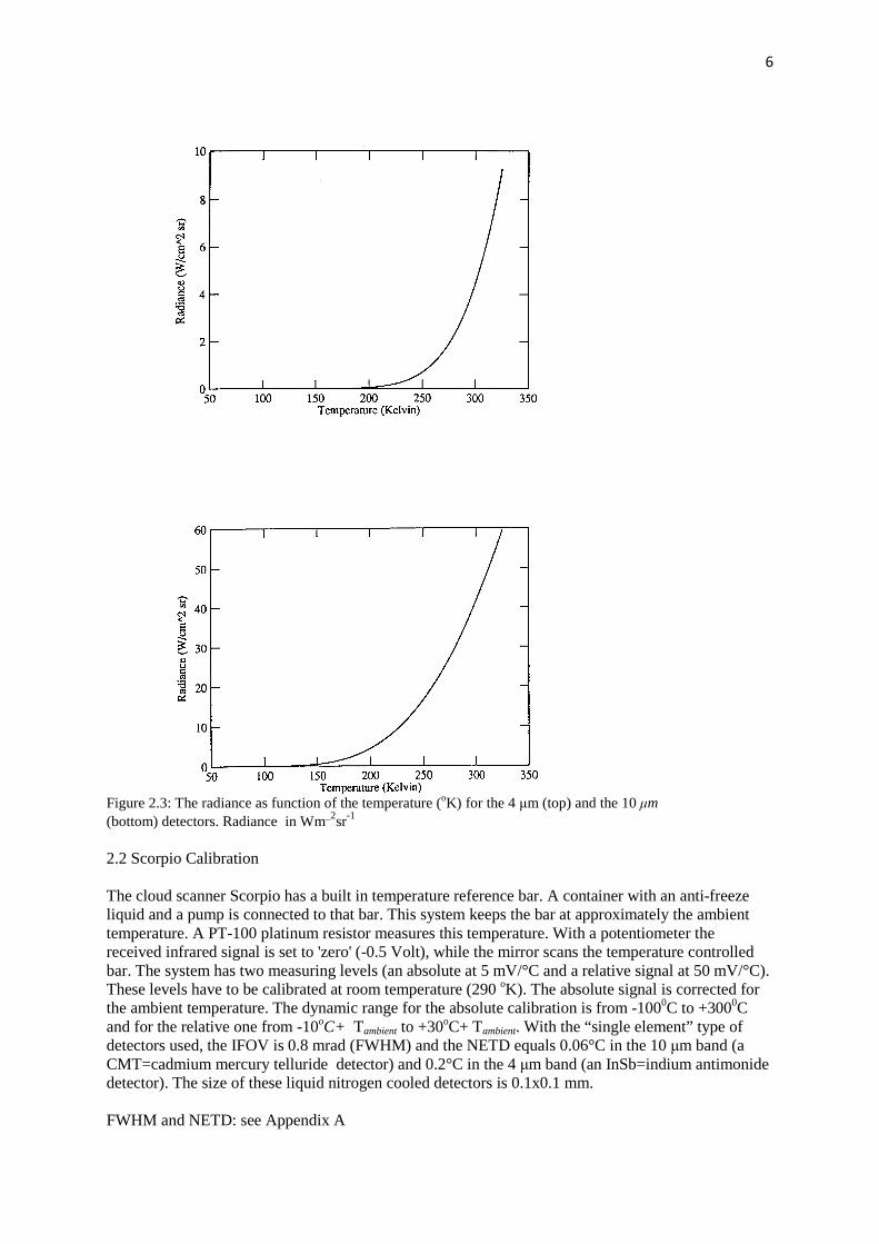
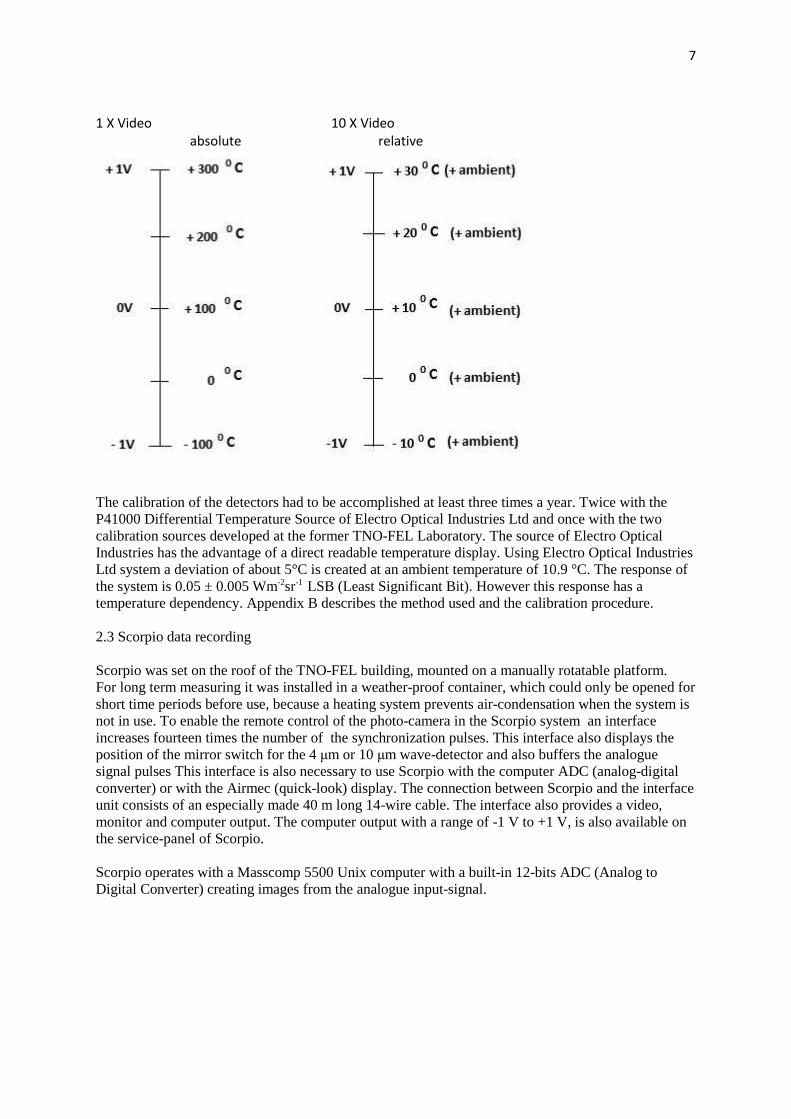
Figure 2.3: The radiance as function of the temperature (oK) for the 4 µm (top) and the 10 µm (bottom) detectors. Radiance in Wm_2sr-1 2.2 Scorpio Calibration The cloud scanner Scorpio has a built in temperature reference bar. A container with an anti-freeze liquid and a pump is connected to that bar. This system keeps the bar at approximately the ambient temperature. A PT-100 platinum resistor measures this temperature. With a potentiometer the received infrared signal is set to 'zero' (-0.5 Volt), while the mirror scans the temperature controlled bar. The system has two measuring levels (an absolute at 5 mV/°C and a relative signal at 50 mV/°C). These levels have to be calibrated at room temperature (290 oK). The absolute signal is corrected for the ambient temperature. The dynamic range for the absolute calibration is from -1000C to +3000C and for the relative one from -10oC+ Tambient to +30oC+ Tambient. With the “single element” type of detectors used, the IFOV is 0.8 mrad (FWHM) and the NETD equals 0.06°C in the 10 µm band (a CMT=cadmium mercury telluride detector) and 0.2°C in the 4 µm band (an InSb=indium antimonide detector). The size of these liquid nitrogen cooled detectors is 0.1x0.1 mm. FWHM and NETD: see Appendix A

7

1 X Video 10 X Video

absolute relative

The calibration of the detectors had to be accomplished at least three times a year. Twice with the P41000 Differential Temperature Source of Electro Optical Industries Ltd and once with the two calibration sources developed at the former TNO-FEL Laboratory. The source of Electro Optical Industries has the advantage of a direct readable temperature display. Using Electro Optical Industries Ltd system a deviation of about 5°C is created at an ambient temperature of 10.9 °C. The response of the system is 0.05 ± 0.005 Wm-2sr-1 LSB (Least Significant Bit). However this response has a temperature dependency. Appendix B describes the method used and the calibration procedure. 2.3 Scorpio data recording Scorpio was set on the roof of the TNO-FEL building, mounted on a manually rotatable platform. For long term measuring it was installed in a weather-proof container, which could only be opened for short time periods before use, because a heating system prevents air-condensation when the system is not in use. To enable the remote control of the photo-camera in the Scorpio system an interface increases fourteen times the number of the synchronization pulses. This interface also displays the position of the mirror switch for the 4 µm or 10 µm wave-detector and also buffers the analogue signal pulses This interface is also necessary to use Scorpio with the computer ADC (analog-digital converter) or with the Airmec (quick-look) display. The connection between Scorpio and the interface unit consists of an especially made 40 m long 14-wire cable. The interface also provides a video, monitor and computer output. The computer output with a range of -1 V to +1 V, is also available on the service-panel of Scorpio. Scorpio operates with a Masscomp 5500 Unix computer with a built-in 12-bits ADC (Analog to Digital Converter) creating images from the analogue input-signal.

8

Each image consists of 2000 lines with 5600 pixels for each line (16.8 Mb of data). The analogue output of Scorpio is -1 to +1 Volt. The ADC input has to be limited between -5 to +5Volt. The ADC has therefore an internal gain control, which can be set to 1, 2,4 and 8 times. Generally the images were obtained using the gain of the ADC set to 8 times. Using such a setting will not exceed the range of the ADC (except measuring direct sunlight). Another possibility is to use the high, relative sensitivity of the system. The ADC gain is than set to 4 times, the analogue signal is still limited between -5 and +5 Volt. However the effective dynamic range of 40°C with this setting can only be used during Summertime. In Winter the difference between the very low air temperature at higher sky levels and the temperature at ground level is too large, the analogue signal will then be limited at -1Volt. The 10 µm detector was mainly used. The 4 µm detector signal contains noise of the motor, which rotates the mirror. This was identified by taken a part of the sky with a uniform distribution. A FFT (Fast Fourier Transformation) of this 512x512 pixels image was generated for both the 10 µm and the 4 µm wavelength. Figure 2.5 shows the amplitude of that FFT. A spike at position 64 is present in the 4 µm FFT-image, caused by the mirror-driving motor. The motor is rotating at a frequency of (25/8) Hz. The image can be corrected for this spike. This gives a better result but the image still contains a lot of other spikes. Figure 2.6 shows the curve for the FFT of a 10 µm image for the same part of the sky. A software package was written in C language at the former TNO-FEL by Mr. R.A.W. Kemp and Mr. A.C. Kruseman to analyze the images and to reduce the quantity of data. The analysis was performed on the built-in “Masscomp” computer. The software on this computer can also be executed on other computers. Together with the computer software, this system is an all-round “all-sky image” scanning-system.

9

Figure 2.4: Schematic overview of the TNO-FEL cloud scanner Scorpio setup.

Figure 2.5: The FFT diagram of a 4 µm image (512x512 pixels) from a part of the sky without objects.

10

Figure 2.6: The FFT of a 10 µm image (512x512 pixels) from a part of the identical sky without objects.

3

11

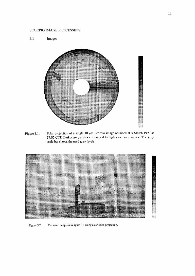
SCORPIO IMAGE PROCESSING 3.1 Images

12

3.2 Image and Clutter processing A number of methods describing clutter had been presented all over the years [1][2]. Clutter is a term used for unwanted echoes in electronic systems, such as IR systems. In infrared measurements of clutter and clouds the mathematical RMS (Root Mean Square) variations, in parts of a recorded IR image, gives the RMS’ value a good estimation for that amount of clutter. For better interpretations the image noise has to be removed from images of homogeneous sky-areas.

13

The created raw SCORPIO-images are sub-divided in cells with n x m pixels. Based on these n x m dimensions, additions over pixels in the cells are performed. The RMS (Root Mean Square) value for

each cell can be calculated for the average radiance intensity µstatic:

A more different method to calculate the average radiance intensity for each pixel µdynamic of a cell with n x m pixels is to calculate the RMS values ( with the same addition over pixels in the cell) for every pixel in that cell, looking at an area of n+2 x m +10 pixels for a 4x12 pixel cell and at n+2 x m + 4 pixels for a 4x6 pixel cell.

In the RMS calculations, the average radiation value of the cell, with locations at every pixel position

(x,y) of that cell was taken in that calculated µdynamic way.

In an area with small variance of radiation the two methods of calculation(µstatic and µdynamic ) have nearly the same result. In a more structured image (clouds, objects) a significant difference in the processed images will be obtained.

14

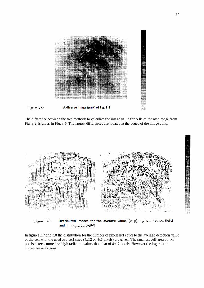
The difference between the two methods to calculate the image value for cells of the raw image from Fig. 3.2. is given in Fig. 3.6. The largest differences are located at the edges of the image cells.

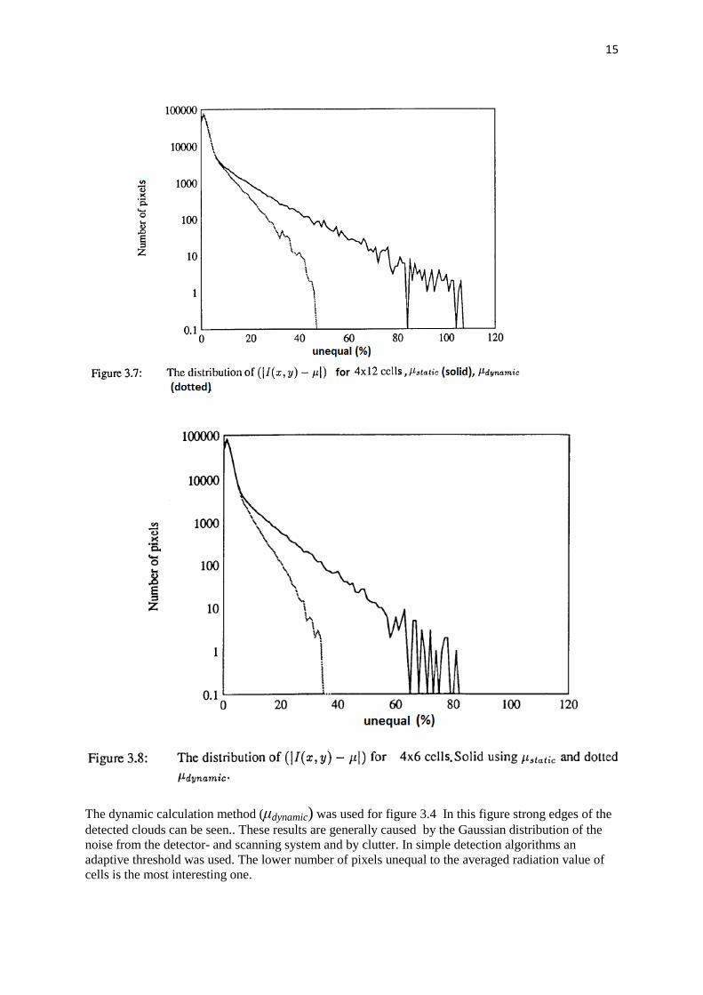
In figures 3.7 and 3.8 the distribution for the number of pixels not equal to the average detection value of the cell with the used two cell sizes (4x12 or 4x6 pixels) are given. The smallest cell-area of 4x6 pixels detects more less high radiation values than that of 4x12 pixels. However the logarithmic curves are analogous.

15

The dynamic calculation method (µdynamic) was used for figure 3.4 In this figure strong edges of the detected clouds can be seen.. These results are generally caused by the Gaussian distribution of the noise from the detector- and scanning system and by clutter. In simple detection algorithms an adaptive threshold was used. The lower number of pixels unequal to the averaged radiation value of cells is the most interesting one.

16

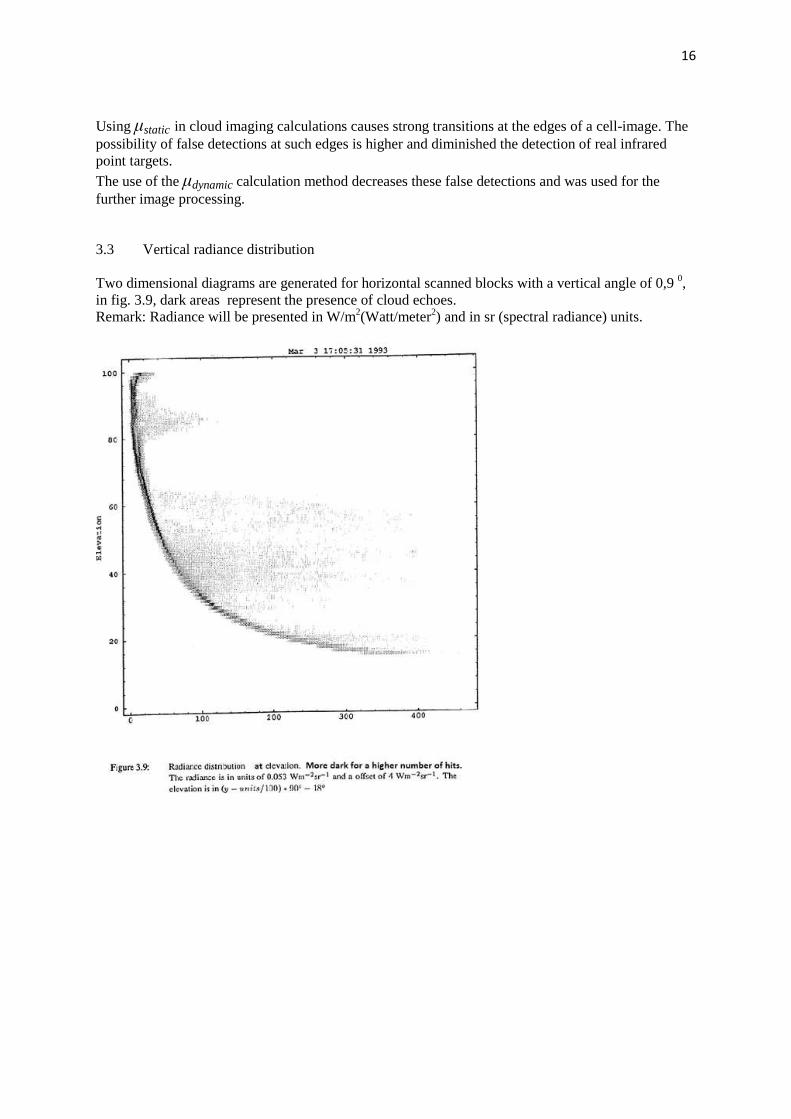
Using µstatic in cloud imaging calculations causes strong transitions at the edges of a cell-image. The possibility of false detections at such edges is higher and diminished the detection of real infrared point targets. The use of the µdynamic calculation method decreases these false detections and was used for the further image processing. 3.3 Vertical radiance distribution Two dimensional diagrams are generated for horizontal scanned blocks with a vertical angle of 0,9 0, in fig. 3.9, dark areas represent the presence of cloud echoes. Remark: Radiance will be presented in W/m2(Watt/meter2) and in sr (spectral radiance) units.

17

Fig 3.10 Clouds distribution (logarithmical plotted).

Horizontal axis in units of 0.027 Wm-2sr-1. The lower radiance black area was caused by the noise of the system

Fig 3.11 Radiance distribution in pixels of fig 3.10. Horizontal axis in units of 0.027 Wm-2sr-1.

18

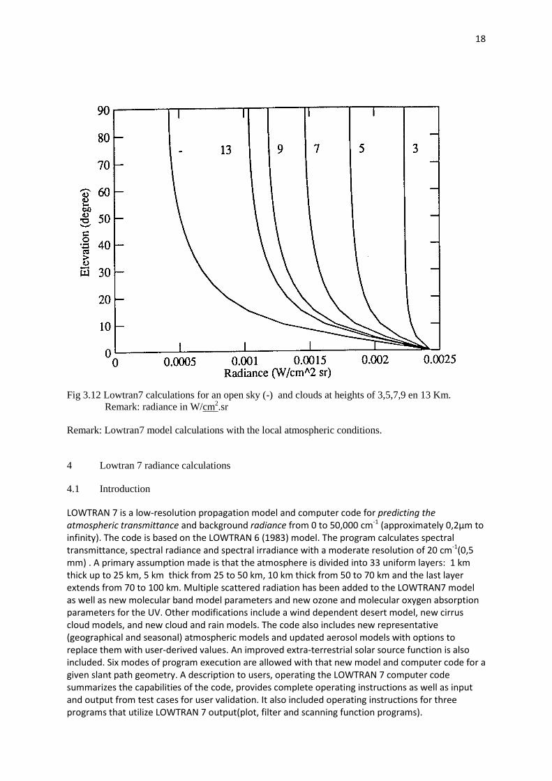
Fig 3.12 Lowtran7 calculations for an open sky (-) and clouds at heights of 3,5,7,9 en 13 Km. Remark: radiance in W/cm2.sr Remark: Lowtran7 model calculations with the local atmospheric conditions. 4 Lowtran 7 radiance calculations 4.1 Introduction LOWTRAN 7 is a low-resolution propagation model and computer code for predicting the

atmospheric transmittance and background radiance from 0 to 50,000 cm-1

(approximately 0,2μm to

infinity). The code is based on the LOWTRAN 6 (1983) model. The program calculates spectral

transmittance, spectral radiance and spectral irradiance with a moderate resolution of 20 cm-1

(0,5

mm) . A primary assumption made is that the atmosphere is divided into 33 uniform layers: 1 km

thick up to 25 km, 5 km thick from 25 to 50 km, 10 km thick from 50 to 70 km and the last layer

extends from 70 to 100 km. Multiple scattered radiation has been added to the LOWTRAN7 model

as well as new molecular band model parameters and new ozone and molecular oxygen absorption

parameters for the UV. Other modifications include a wind dependent desert model, new cirrus

cloud models, and new cloud and rain models. The code also includes new representative

(geographical and seasonal) atmospheric models and updated aerosol models with options to

replace them with user-derived values. An improved extra-terrestrial solar source function is also

included. Six modes of program execution are allowed with that new model and computer code for a

given slant path geometry. A description to users, operating the LOWTRAN 7 computer code

summarizes the capabilities of the code, provides complete operating instructions as well as input

and output from test cases for user validation. It also included operating instructions for three

programs that utilize LOWTRAN 7 output(plot, filter and scanning function programs).

19

The execution of the LOWTRAN7 (based on program-language FORTRAN) program was done by the

input of cards. These Hollerith cards, as input for a former card-reader , were built up with 80

columns of instruction fields.

Some various quantities to be specified on each of the five control cards along with the fourteen

optional cards are given on the first three program-input cards.

Card1 contains the following items:

MODEL, ITYPE, IEMSCT, IMULT,M1, M2, M3, M4, M5, M6, MDEF , IM, NOPRT, TBOUND, SALB

FORMAT (13I5, F8.3, F7.2)

MODEL: selects one of the six geographical-seasonal model atmospheres or specifies that user-

defined meteorological data are to be used.

ITYPE: indicates the type of atmospheric path.

IEMSCT: determines the mode of execution of the program.

IMULT: determines execution of multiple scattering.

M1, M2, M3, M4, M5 and M6 are used to modify or supplement the altitude profiles of temperature

and pressure, water vapor, ozone, methane, nitrous oxide and carbon monoxide from the

atmosphere models stored in the program.

MDEF uses the default(U.S. Standard) profiles for the remaining species.

For normal operation of program (MODEL 1 to 6)

Set M1=M2=M3=0, M4=M5=M6=MDEF=0

IM: =1, when user input data are to be read initially.

NOPRT: =0, for normal operation of program. Controls TAPE6 output.

TBOUND: =0.000

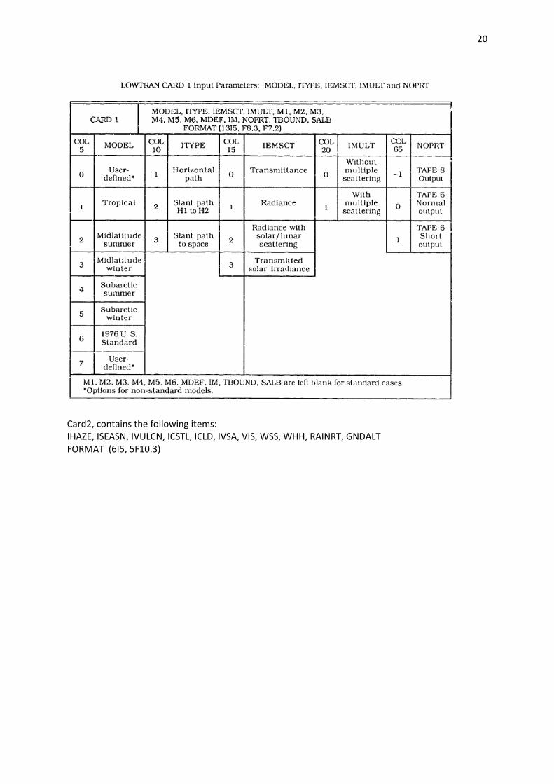
An example for LOWTRAN CARD 1 with Input parameters: MODEL, ITYPE,IEMSCT, IMULT and NOPRT

20

Card2, contains the following items:

IHAZE, ISEASN, IVULCN, ICSTL, ICLD, IVSA, VIS, WSS, WHH, RAINRT, GNDALT

FORMAT (6I5, 5F10.3)

21

22

Card2B, contains the following items: (if IVSA =1)

ZCVSA, ZTVSA, ZINVSA

FORMAT (3F10.3)

4.2 Input data Relevant meteorological data had to be used. These data were only available at ground level.

An example of a tape 5(Lowtran7 ) input file

As basic model a path from 10m latitude to aerial space, with the mid latitude winter

circumstances, in the range of 770 to 1200 cm-1

was taken. Also in Lowtran7 the single- or multiple

scattering mode can be selected (Fig. 4.1). The multiple scattering mode was from now on used.

Remark: Also a newer version of LOWTRAN7, MODTRAN was used. MODTRAN results in a small

difference in radiance values at low heights, at higher elevations the difference can rise to

0.05 W-2

.sr-1

.

4.3 Simulation for clouds radiances Three ways to model the radiance for a full sky clouds layer at a specific height are:

1. Calculate a slant path to the clouds height using the clouds as a black body with the temperature of that clouds layer. 2. Read another layer model and set the relative humidity (RH) to 100 % for that cloud level, the equivalent liquid water content > 10 and parameter IHA1(Aerosol model extinction and meteorological range control for that altitude) of card 2C3 to a fog type. Each entry in the TAPE5 file will use that profile. The LOWTRAN option IM=1 of card 1 can only be used while changing the elevation. 3. Using the clouds models in Lowtran. This method has the disadvantage that only 8 clouds models can be specified. Five lower level models and three cirrus-clouds models. Comparing real radiance profiles with predictions, only the methods 1and 2 can be used. In the second method an atmospheric profile is necessary. The resulting radiance curves deliver a deviation of 1.5 Wm -2sr -1. Figure 4.2 (method 1) gives the radiance curves in a mid latitude winter and figure 4.3 the curves in a mid latitude summer. The values of clouds levels above 7 km are not realistic at 52°N geographical latitude. These are only shown to give an impression. Clouds above 7 km are cirrus clouds. The concerning scattering and transmission of cirrus clouds differ from lower level clouds. LOWTRAN7 contains 3 special models for cirrus clouds (card 2: ICLD 18, 19,20). Using card 2A the clouds altitude (CALT) and thickness (CTHIK) can be set. Figure 4.4 shows those three curves. The radiance curves of cirrus clouds are almost identical to that of an open sky.

23

Fig 4.2 Mid latitude winter-radiation of Fig 4.3 Mid latitude summer-radiation of

clouds at different heights (Km) clouds at different heights (Km)

and no-clouds radiation and no clouds

24

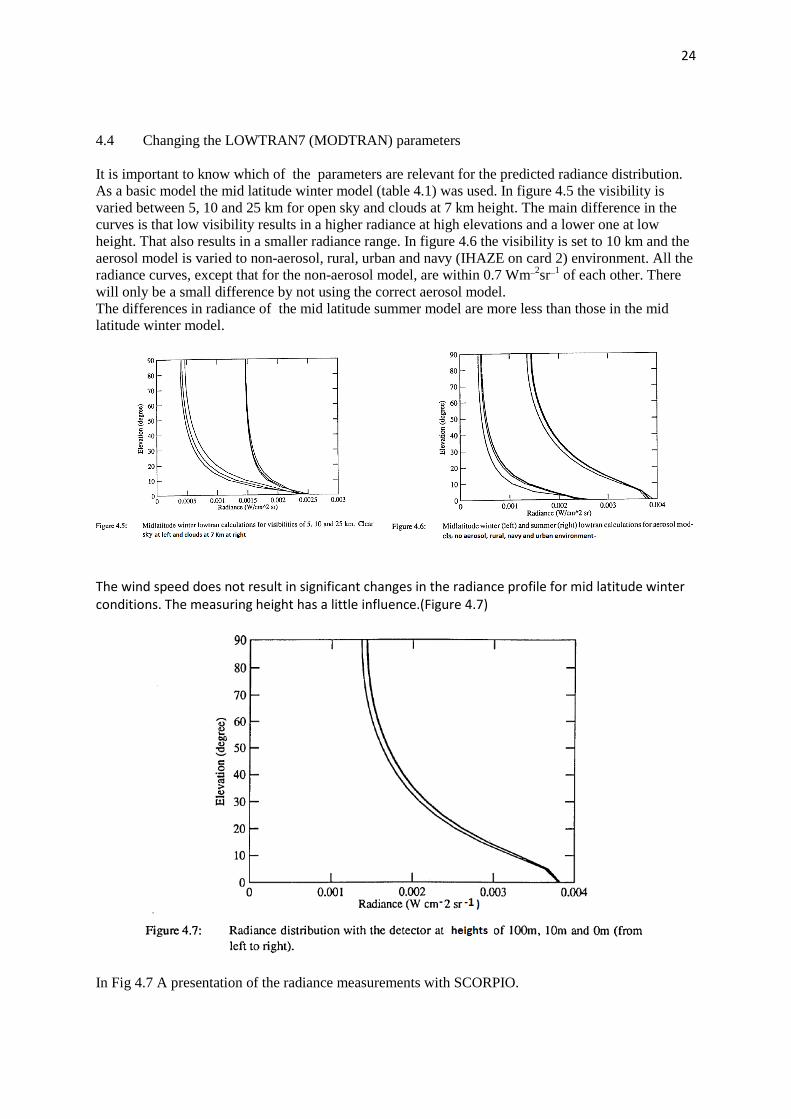
4.4 Changing the LOWTRAN7 (MODTRAN) parameters It is important to know which of the parameters are relevant for the predicted radiance distribution. As a basic model the mid latitude winter model (table 4.1) was used. In figure 4.5 the visibility is varied between 5, 10 and 25 km for open sky and clouds at 7 km height. The main difference in the curves is that low visibility results in a higher radiance at high elevations and a lower one at low height. That also results in a smaller radiance range. In figure 4.6 the visibility is set to 10 km and the aerosol model is varied to non-aerosol, rural, urban and navy (IHAZE on card 2) environment. All the radiance curves, except that for the non-aerosol model, are within 0.7 Wm_2sr_1 of each other. There will only be a small difference by not using the correct aerosol model. The differences in radiance of the mid latitude summer model are more less than those in the mid latitude winter model.

The wind speed does not result in significant changes in the radiance profile for mid latitude winter

conditions. The measuring height has a little influence.(Figure 4.7)

In Fig 4.7 A presentation of the radiance measurements with SCORPIO.

25

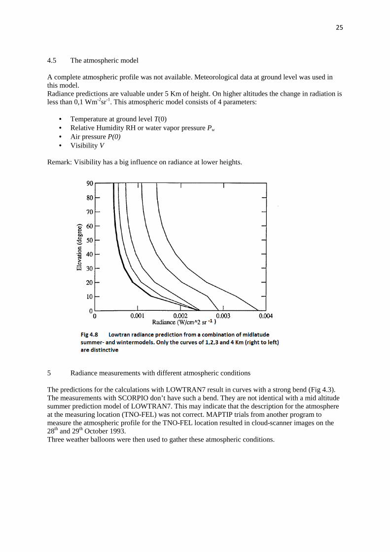
4.5 The atmospheric model A complete atmospheric profile was not available. Meteorological data at ground level was used in this model. Radiance predictions are valuable under 5 Km of height. On higher altitudes the change in radiation is less than 0,1 Wm-2sr-1. This atmospheric model consists of 4 parameters:

• Temperature at ground level T(0) • Relative Humidity RH or water vapor pressure Pw • Air pressure P(0) • Visibility V

Remark: Visibility has a big influence on radiance at lower heights.

5 Radiance measurements with different atmospheric conditions The predictions for the calculations with LOWTRAN7 result in curves with a strong bend (Fig 4.3). The measurements with SCORPIO don’t have such a bend. They are not identical with a mid altitude summer prediction model of LOWTRAN7. This may indicate that the description for the atmosphere at the measuring location (TNO-FEL) was not correct. MAPTIP trials from another program to measure the atmospheric profile for the TNO-FEL location resulted in cloud-scanner images on the 28th and 29th October 1993. Three weather balloons were then used to gather these atmospheric conditions.

26

27

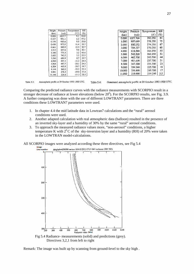
Comparing the predicted radiance curves with the radiance measurements with SCORPIO result in a stronger decrease of radiance at lower elevations (below 200). For the SCORPIO results, see Fig. 3.9. A further comparing was done with the use of different LOWTRAN7 parameters. There are three conditions these LOWTRAN7 parameters were used.

1. In chapter 4.4 the mid latitude data in Lowtran7 calculations and the “rural” aerosol conditions were used.

2. Another adapted calculation with real atmospheric data (balloon) resulted in the presence of an inverted sky-layer and a humidity of 30% by the same “rural” aerosol conditions.

3. To approach the measured radiance values more, “non-aerosol” conditions, a higher temperature K with 20 C of the sky-inversion layer and a humidity (RH) of 20% were taken in the LOWTRAN model-calculations.

All SCORPIO images were analyzed according these three directives, see Fig 5.4

Fig 5.4 Radiance- measurements (solid) and predictions (grey). Directives 3,2,1 from left to right Remark: The image was built up by scanning from ground-level to the sky high .

28

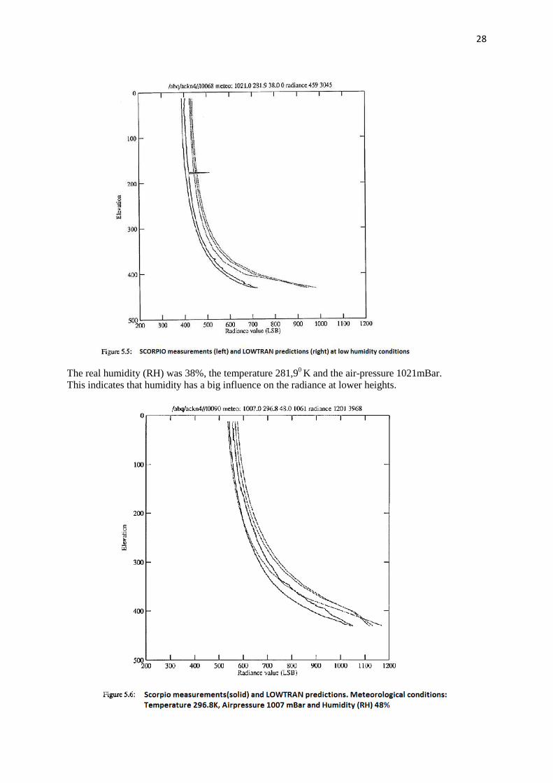
The real humidity (RH) was 38%, the temperature 281,90 K and the air-pressure 1021mBar. This indicates that humidity has a big influence on the radiance at lower heights.

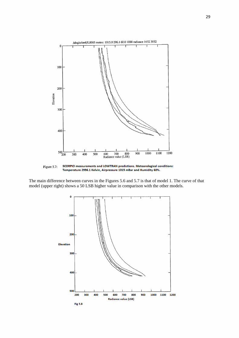
29

The main difference between curves in the Figures 5.6 and 5.7 is that of model 1. The curve of that model (upper right) shows a 50 LSB higher value in comparison with the other models.

30

Fig 5.9. Conclusions from the measurements and the prediction calculations shown in the figures 5.2 to 5.9 are:

• Model 1 can only be used for a prediction of radiance in a horizontal area all round at ground level

• Model 2 delivers good matches with the real measurements under the same meteorological circumstances. The influence of humidity at ground level has a great affect in the difference of radiance.

• Model 3 calculations correspond well with the SCORPIO measuring results. Humidity plays a minor role for the predictions with this model.

By using this model 3 a number of atmospheric parameters may be changed to match the real atmospheric conditions. Remark: Predictions for the radiance under 5 Km height can be calculated with realistic results. 6 IMAGE ANALYSIS 6.1 The analysis of the generated images is to divide in three parts:

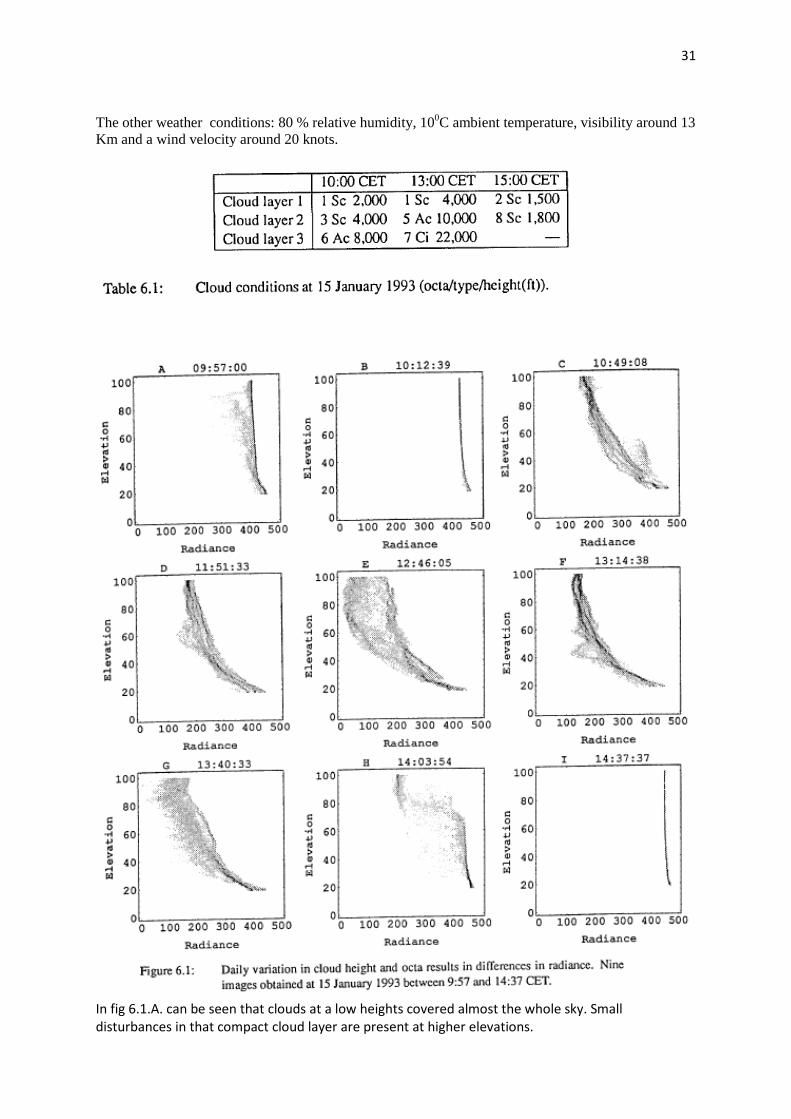
On profile, clutter and clouds. The analysis of the radiance profile is described in Chapter 5. The clutter and clouds influences on the IR radiation are described in the following paragraphs. During day-time the conditions of the atmosphere may change significantly. The presence of clouds will also influence the radiance values to be measured. An example for this influence is given in the Fig 6.1. Clutter may prevent the detection and identification of objects within that clutter in a common way. Fig 6.1 presents in nine figures the recorded radiances representing the clouds on the 15th of January 1993, between 9:57 CET and 14:37 CET ( Central European Time). The cloud conditions were also recorded by the meteorological institute (KNMI) in De Bilt (see table 6.1).

31

The other weather conditions: 80 % relative humidity, 100C ambient temperature, visibility around 13 Km and a wind velocity around 20 knots.

In fig 6.1.A. can be seen that clouds at a low heights covered almost the whole sky. Small

disturbances in that compact cloud layer are present at higher elevations.

32

About 15 minutes later (Fig 6.1.B.) the whole sky was covered. According the available

meteorological data, the height of that stratocumulus (Sc) clouds layer was at about 4000Ft.

In Fig 6.1.C. (50 minutes later) and Fig 6.1.D. (after 2 hours) that clouds layer was dissolved and an

altocumulus (Ac) layer covered the sky at about 10.000Ft of height with some distortions (Fig

6.1.D.).

Around 13:00 CET that day the layer at 10.000Ft covered 5 octa (level of sky-covering) of the sky. In

Fig 6.1.E. a cirrus(Ci) cloud layer at 22.000Ft height of 7 octa was present.

Fig 6.1.F. en Fig 6.1.G. present an altocumulus layer covering almost the whole sky.

In Fig 6.1.G. radiance presentations at all heights are to be seen. In Fig 6.1.H. the sky was almost

covered with stratocumulus clouds. Just above the location of the TNO-FEL building a gap in those

clouds gives the probability to see the altocumulus layer above the stratocumulus clouds. In the

called Fig 6.1.H. these layers can be distinguished. From 00 to 50

0 of elevation the stratocumulus

clouds and from 650 to 72

0 of elevation the altocumulus clouds.

In fig 6.1.I. the stratocumulus clouds (lower height) covered the whole sky. In comparing the figures

of 6.1.B. and 6.1.I. the clouds in Fig 6.1.I. deliver higher radiance values . Those figures are in

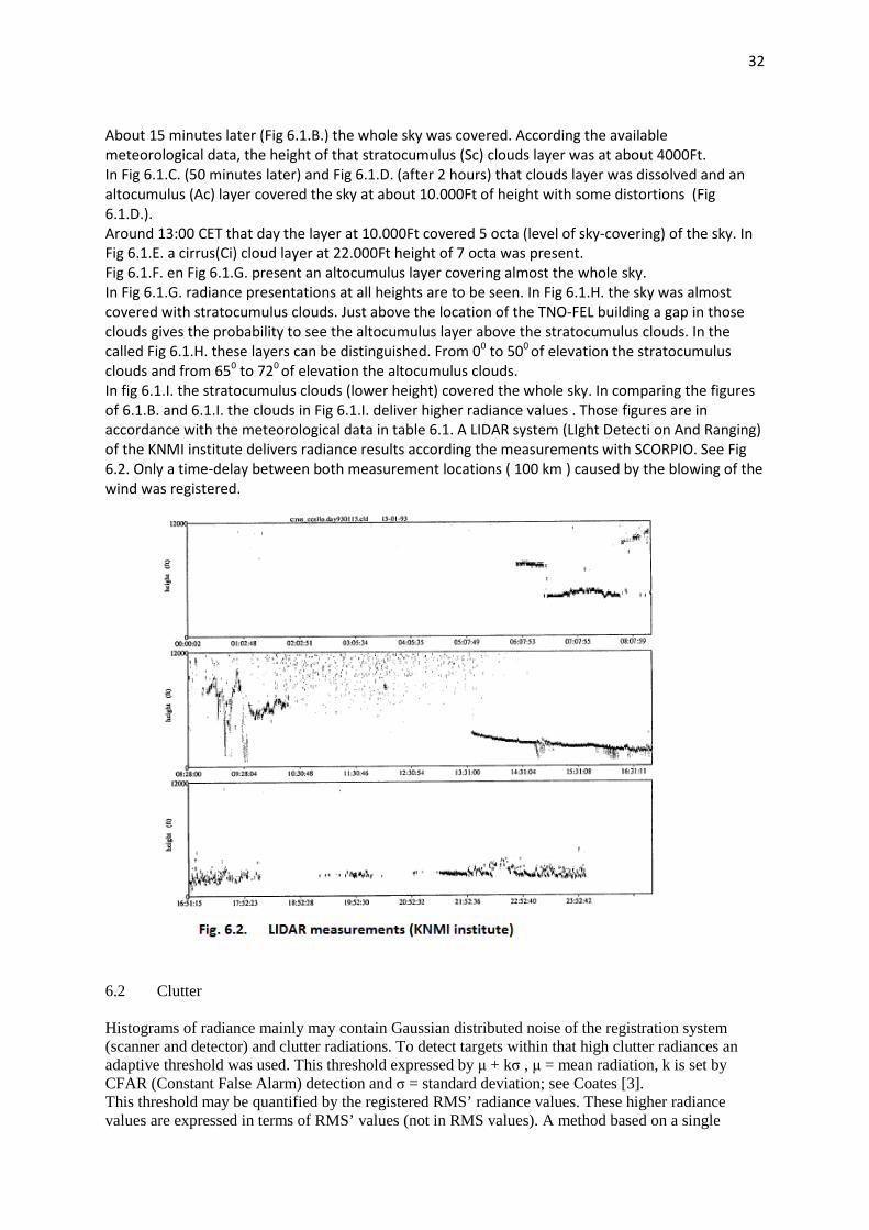
accordance with the meteorological data in table 6.1. A LIDAR system (LIght Detecti on And Ranging)

of the KNMI institute delivers radiance results according the measurements with SCORPIO. See Fig

6.2. Only a time-delay between both measurement locations ( 100 km ) caused by the blowing of the

wind was registered.

6.2 Clutter Histograms of radiance mainly may contain Gaussian distributed noise of the registration system (scanner and detector) and clutter radiations. To detect targets within that high clutter radiances an adaptive threshold was used. This threshold expressed by µ + kσ , µ = mean radiation, k is set by CFAR (Constant False Alarm) detection and σ = standard deviation; see Coates [3]. This threshold may be quantified by the registered RMS’ radiance values. These higher radiance values are expressed in terms of RMS’ values (not in RMS values). A method based on a single

33

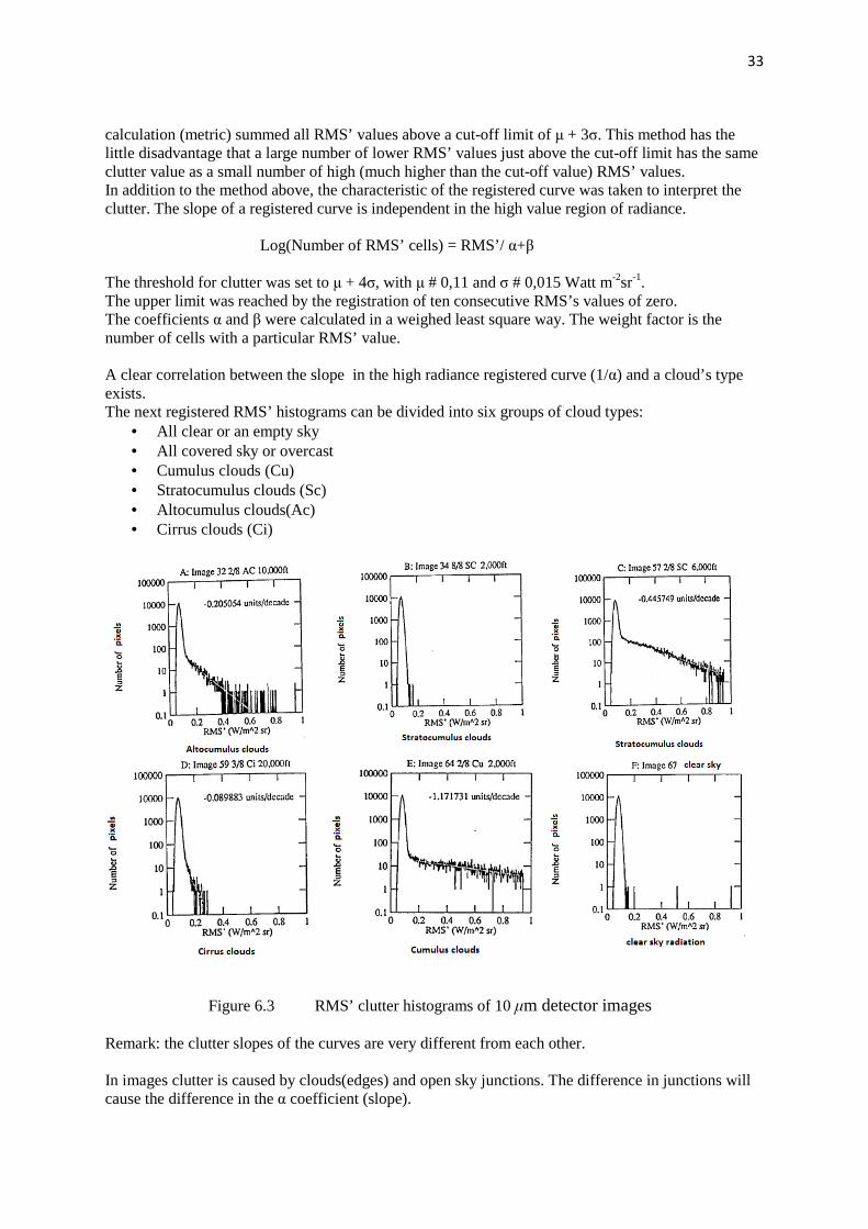
calculation (metric) summed all RMS’ values above a cut-off limit of µ + 3σ. This method has the little disadvantage that a large number of lower RMS’ values just above the cut-off limit has the same clutter value as a small number of high (much higher than the cut-off value) RMS’ values. In addition to the method above, the characteristic of the registered curve was taken to interpret the clutter. The slope of a registered curve is independent in the high value region of radiance. Log(Number of RMS’ cells) = RMS’/ α+β The threshold for clutter was set to µ + 4σ, with µ # 0,11 and σ # 0,015 Watt m-2sr-1. The upper limit was reached by the registration of ten consecutive RMS’s values of zero. The coefficients α and β were calculated in a weighed least square way. The weight factor is the number of cells with a particular RMS’ value. A clear correlation between the slope in the high radiance registered curve (1/α) and a cloud’s type exists. The next registered RMS’ histograms can be divided into six groups of cloud types:

• All clear or an empty sky • All covered sky or overcast • Cumulus clouds (Cu) • Stratocumulus clouds (Sc) • Altocumulus clouds(Ac) • Cirrus clouds (Ci)

Figure 6.3 RMS’ clutter histograms of 10 µm detector images Remark: the clutter slopes of the curves are very different from each other. In images clutter is caused by clouds(edges) and open sky junctions. The difference in junctions will cause the difference in the α coefficient (slope).

34

In the diagrams the value of α is also given. Clutter radiances are mostly present in the lower elevation regions. The number of clutter values are determined by the thickness of the cloud cover. To recognize radiating objects in the registered radiances, the pixel radiance values should elapse with 1,5 Wm_2sr_1 for the first 00 till 100 of elevation, with 1,3 Wm_2sr_1 for the next 100 till 150 and with 1,5 Wm_2sr_1 from 150 until maximum of elevation. Pixel values exceeding these values may be separate radiating objects.

35

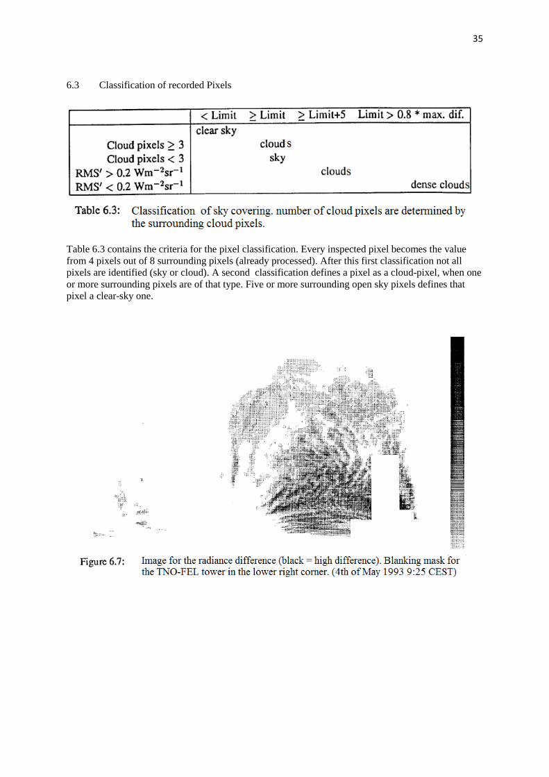
6.3 Classification of recorded Pixels

Table 6.3 contains the criteria for the pixel classification. Every inspected pixel becomes the value from 4 pixels out of 8 surrounding pixels (already processed). After this first classification not all pixels are identified (sky or cloud). A second classification defines a pixel as a cloud-pixel, when one or more surrounding pixels are of that type. Five or more surrounding open sky pixels defines that pixel a clear-sky one.

36

Fig.6.8. Black indicates dense clouds. Fig. 6.8 shows the image of Fig. 6.7 after classification The difference in radiation between the junctions of a cloud and the center of the cloud (density) can be used to calculate the height of that cloud cover. If more layers of that cloud cover exist the radiance distribution (RMS’ values) cannot deliver a solution to calculate the height of that cover. Only two or more distinctive cloud heights can deliver the height of those covers. For a better indication of the cloudiness the scanner images, which are only recording for a few times, can be processed with a weight factor. Low elevation radiances in the image have a higher factor. 6.4 IR object(s) to detect A subsonic rocket will be used as an example. The IR radiance of the rocket is 50 Wm-2sr-1 at an ambient temperature of 2800 Kelvin in the 10 µm band. The radiance of a pixel of that object is:

A is the area of the object, α is the IFOV (Instantaneous Field Of View), R is the detection-range,

Ltarget is the radiance of the target, τ is the transmission through the path, Lbackground is the radiance

of the sky and Lforeground is the radiance of the air between detector and object. The contrast of the pixel:

37

The foreground contribution in that contrast must be between Lbackground and zero. A Lforeground of zero will result in a maximum of contrast. For a horizontal path with a range of > 5Km the

contribution of radiance will be in the order of Lbackground .

The contrast also depends on the NEI of the system and S/N ratio.

The real contrast value is determined by the IVOF (α), the range (R) and the transmission (τ).

SCORPIO has an IVOF of 0.8 mrad, an irradiance noise (NEI related) of 0,11 Wm-2sr-1 and an α of 0,015 Wm-2sr-1. In a clear sky, pixels with a RMS value > 0,2 Wm-2sr-1 are radiating objects (see Fig. 6.3). The radiance contribution of that object in a pixel of a cell with a RMS’s value of 0,2 Wm-2sr-1 is then 1(one) Wm-2sr-1. The difference in radiance calculated is:

n= number of pixels in one cell (4x12), µ = averaged radiation value in the cell, δ = difference in radiation in a pixel to get a RMS’ value of ∆. LSB (Least Significant Bits) calculations were used. 1 LSB = 0,05 Wm-2sr-1 for absolute sensitivity of the system and 8 times gain-control for the ADC gain-conversion.

The NEI factor has a value of 2LSB’s. δ incorporates the change in the average radiance µ with an extra radiance contribution. The equation than:

Using n >>1

For the RMS’ value of 0,2 Wm-2sr-1 = 4 LSB digits. A ∆ value of 4 results in a value for δ = 22LSB digits of 1 Wm-2sr-1 units. The range of a single target then can be detected is 6 Km (τ =0,5 and Lbackground = 30 Wm-2sr-1). SCORPIO is too slow for direct processing those pixel radiances. The processing needed to do so is than δ > NEI + kσ, for k = 5, δ = 0,185 Wm-2sr-1 corresponding 4 LSB digits. 7 Conclusions SCORPIO can obtain a large amount of data sets of nearly all-sky infrared images. These sets can be used to set-up statistical data. To analyze these data a Masscomp 5500 UNIX computer was used. The

38

data smoothed from unwanted radiation from buildings and clouds was then analyzed for clutter content. These RMS clutter calculations were done with a dynamic averaged background. Also SCORPIO can be used to determine cloud heights and the art of clouds. Clutter may be caused by clouds. The expected clutter contribution can be used for the evaluation of target detection algorithms. Also this contribution can be used to adjust threshold levels. A model was made for a radiance profile of the first 5 Km of the atmosphere. A “non-aerosol” model of the LOWTRAN modeling software was used. Using this model resulted in good matches with the measures of SCORPIO. Also this model resulted in better predictions for non-horizontal path radiances. For a correct detection of long range infrared targets a real description of the atmosphere (humidity) is needed. A great contribution for the improvement of the clutter mathematics was delivered with the IRSCAN evaluation trials in 1992. Profile analysis on elevation had the result of more accurate clutter first order estimates near the horizon. This clutter determination can also be used for the background modeling of the IRST models for a better performance.

Notes for operation with SCORPIO

A.1 External noise sources Operating SCORPIO, the sensitivity for external Electro-Magnetic field became obvious. The nearby FELSTAR radar-system of the FEL-Laboratories (see Fig. A.1) was one of the sources for EM.

Fig. A.1 Increases of noise caused by the FELSTAR radar-system An HF antenna above SCORPIO also produced noise in SCORPIO. The noise level without an active EM apparatus is about 0,1 Wm-2sr-1. With an active broadcasting HF antenna the noise level raised at 0,3 Wm-2sr-1.

39

A.2 Overload by the sun The heat of the sun causes during a direct view of SCORPIO at the sun an overload for the detectors. To avoid this effect the reference bar is used to obscure the sun while passing by. A.3 ADC Conversion One of the Analogue Digital Converters did not operate correctly. The conversion for the 4th bit was too late. Values of modulo 16 in the IR images were incorrect. A.4 Positioning of SCORPIO For the images obtained with SCORPIO, the whole scanning system has to be positioned in a precisely horizontal position. Indices

1) The DuDa (Dutch-Danish) scanner is an instrument to gather quantitative infrared signatures. The total field of view of 30 horizontal x 150 vertical is scanned within 4 sec, simultaneously with a 5µ and 10 µ detector. With the instantaneous field of view of 1 mRad a noise equivalent temperature difference of 0.1 k and 0.03 k is achieved. The signals can be recorded analogically or digitally, with a computer, on diskette or on tape. A large format display system was also available.

2) Constant false alarm rate (CFAR) detection refers to a common form of adaptive algorithm used in radar systems to detect target returns against a background of noise, clutter and interference.

Principle of CFAR

In the radar receiver the returning echoes are typically received by the antenna, amplified, down-converted and then passed through detector circuitry, that extracts the envelope of the signal (known as the video signal). This video signal is proportional to the power of the received echo and comprises the wanted echo signal and the unwanted power from internal receiver noise and external clutter and interference.

However, in most fielded systems, unwanted clutter and interference sources mean that the noise level changes both spatially and temporally. In this case, a changing threshold can be used, where the threshold level is raised and lowered to maintain a constant probability of false alarm. This is known as constant false alarm rate (CFAR) detection.

Cell-averaging CFAR

40

Constant False Alarm Rate(CFAR). The center is the cell under test. The two adjacent cells are added and multiplied by a constant to establish a threshold. Detection occurs when the cell under test exceeds the threshold.

In most simple CFAR detection schemes, the threshold level is calculated by estimating the level of the noise floor around the cell under test (CUT). This can be found by taking a block of cells around the cell under test (CUT) and calculating the average power level. To avoid corrupting this estimate with power from the CUT itself, cells immediately adjacent to the CUT are normally ignored (and referred to as "guard cells"). A target is declared present in the CUT if it is both greater than all its adjacent cells and greater than the local average power level. The estimate of the local power level may sometimes be increased slightly to allow for the limited sample size. This simple approach is called a cell-averaging CFAR (CA-CFAR).

Other related approaches calculate separate averages for the cells to the left and right of the CUT, and then use the greatest-of or least-of these two power levels to define the local power level. These are referred to as greatest-of CFAR (GO-CFAR) and least-of CFAR (LO-CFAR) respectively, and can improve detection when immediately adjacent to areas of clutter.

Appendix A

FWHM

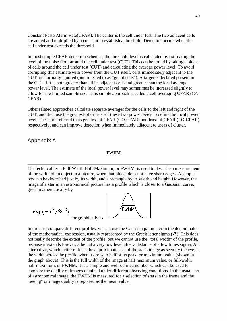
The technical term Full-Width Half-Maximum, or FWHM, is used to describe a measurement of the width of an object in a picture, when that object does not have sharp edges. A simple box can be described just by its width, and a rectangle by its width and height. However, the image of a star in an astronomical picture has a profile which is closer to a Gaussian curve, given mathematically by

or graphically as

In order to compare different profiles, we can use the Gaussian parameter in the denominator of the mathematical expression, usually represented by the Greek letter sigma (). This does not really describe the extent of the profile, but we cannot use the "total width" of the profile, because it extends forever, albeit at a very low level after a distance of a few times sigma. An alternative, which better reflects the approximate size of the star's image as seen by the eye, is the width across the profile when it drops to half of its peak, or maximum, value (shown in the graph above). This is the full width of the image at half maximum value, or full-width half-maximum, or FWHM. It is a simple and well-defined number which can be used to compare the quality of images obtained under different observing conditions. In the usual sort of astronomical image, the FWHM is measured for a selection of stars in the frame and the "seeing" or image quality is reported as the mean value.

41

NETD (Noise Equivalent Temperature Difference) is a measure of the sensitivity of a detector of thermal radiation in the infrared, terahertz radiation or microwave radiation parts of the electromagnetic spectrum.

Appendix B

Calibration of SCORPIO The calibration was performed with the Electro Optical Industries (EOI) P14000 differential temperature source. This system consists of a temperature controlled center plate and two side plates at ambient temperature. The system was positioned at a 10 meter distance in front of SCORPIO. The radiance transmission is > 0,999% over this short path. The center plate was set at +50C. The temperature of the side plates was measured at the left one. An image was generated by SCORPIO with a selection of that image for the position of the center plate. That area of selection had dimensions of 25X25 pixels. Selections of 10 to 16 pixels were then made in the horizontal en vertical direction over the image of the surfaces of the center and outer plate. The average value and the standard deviation σ were then calculated (see tables B.1 and B.2).

.

From those measurements it became clear that the differences were too large. These could not only be caused by the noise of the system . There must be a correlation between the outside temperature and the response of SCORPIO. SCORPIO corrects its signal with the reference signal for the dark current of the detector generated during the passing of the reference bar. The temperature of the bar is measured with a temperature sensitive resistor (Pt-100) and added to the IR signal. That value is linear to the temperature and set on 5 mV/0K. The temperature response of SCORPIO (between 2,5 and 3,2mV/0K) can be calculated from:

42

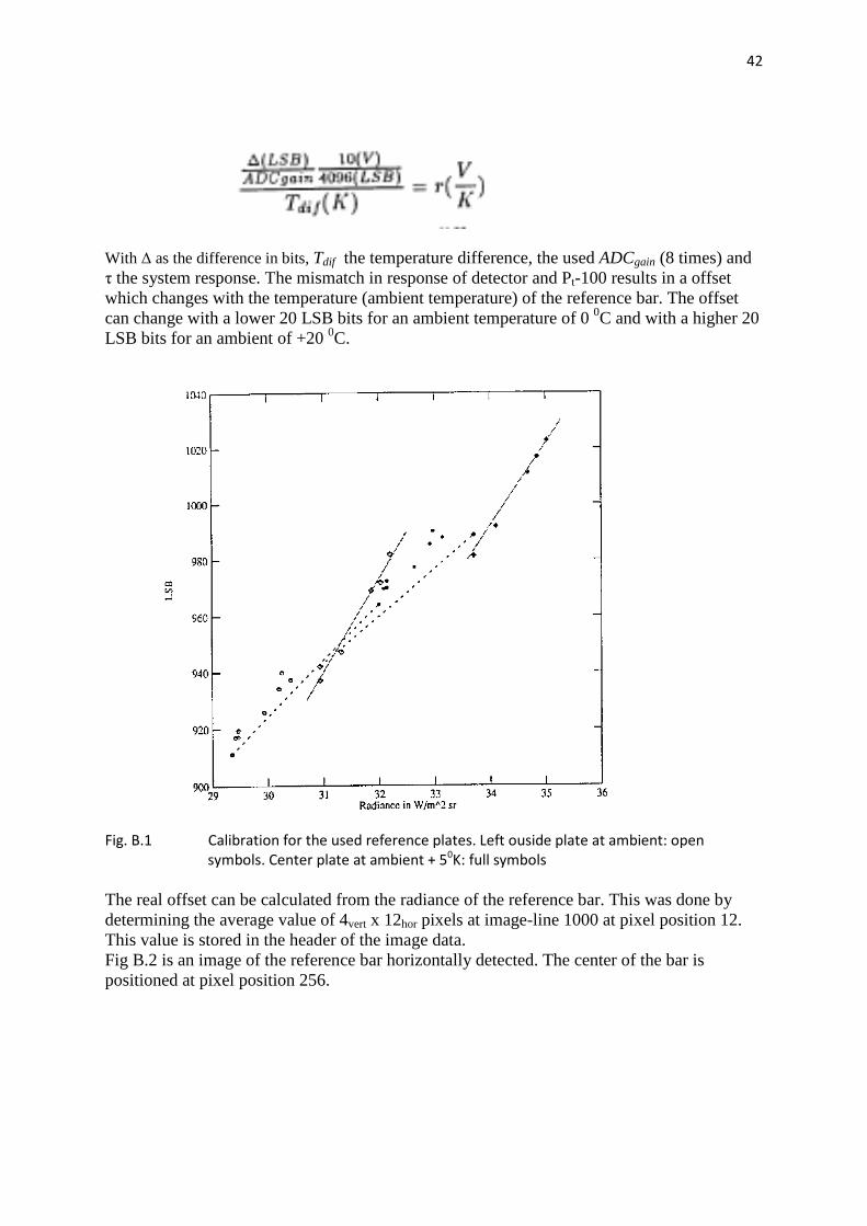
With ∆ as the difference in bits, Tdif the temperature difference, the used ADCgain (8 times) and τ the system response. The mismatch in response of detector and Pt-100 results in a offset which changes with the temperature (ambient temperature) of the reference bar. The offset can change with a lower 20 LSB bits for an ambient temperature of 0 0C and with a higher 20 LSB bits for an ambient of +20 0C.

Fig. B.1 Calibration for the used reference plates. Left ouside plate at ambient: open

symbols. Center plate at ambient + 50K: full symbols

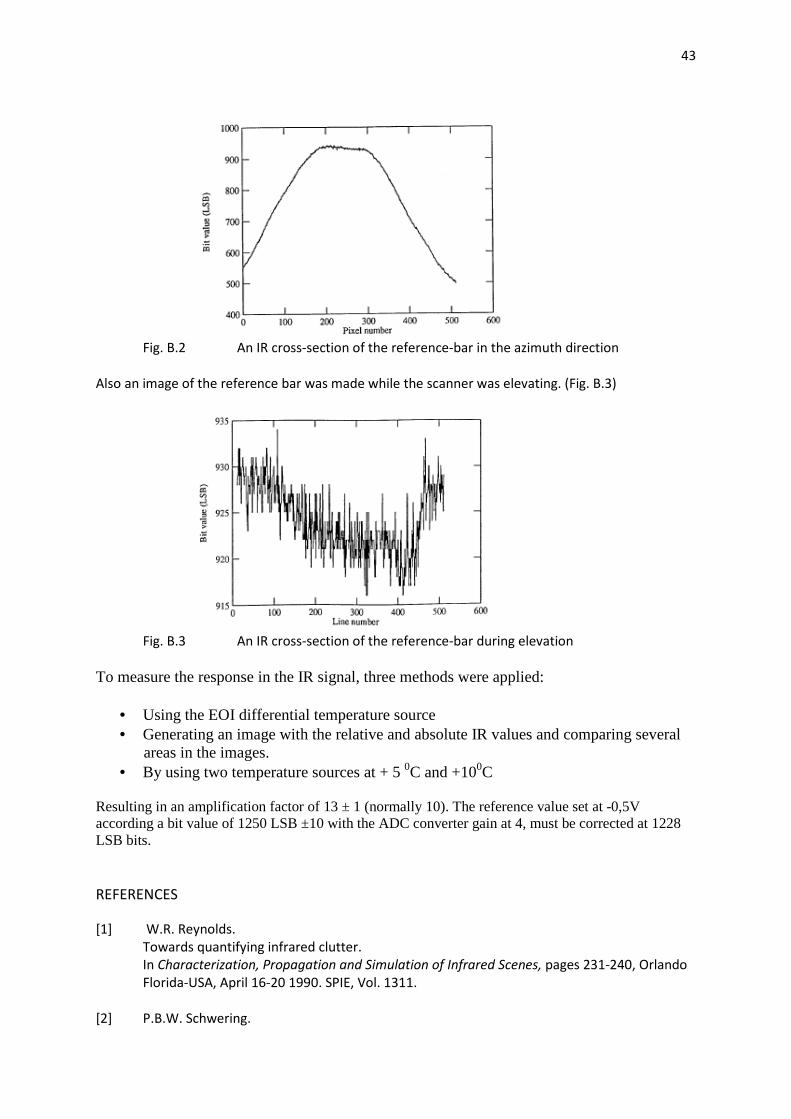
The real offset can be calculated from the radiance of the reference bar. This was done by determining the average value of 4vert x 12hor pixels at image-line 1000 at pixel position 12. This value is stored in the header of the image data. Fig B.2 is an image of the reference bar horizontally detected. The center of the bar is positioned at pixel position 256.

43

Fig. B.2 An IR cross-section of the reference-bar in the azimuth direction

Also an image of the reference bar was made while the scanner was elevating. (Fig. B.3)

Fig. B.3 An IR cross-section of the reference-bar during elevation

To measure the response in the IR signal, three methods were applied:

• Using the EOI differential temperature source • Generating an image with the relative and absolute IR values and comparing several

areas in the images. • By using two temperature sources at + 5 0C and +100C

Resulting in an amplification factor of 13 ± 1 (normally 10). The reference value set at -0,5V according a bit value of 1250 LSB ±10 with the ADC converter gain at 4, must be corrected at 1228 LSB bits.

REFERENCES

[1] W.R. Reynolds.

Towards quantifying infrared clutter.

In Characterization, Propagation and Simulation of Infrared Scenes, pages 231-240, Orlando

Florida-USA, April 16-20 1990. SPIE, Vol. 1311.

[2] P.B.W. Schwering.

44

Characterization of infrared cloud background clutter.

In Characterization, Propagation and Simulation of Sources and Backgrounds II , pages 311-

322, Orlando Florida-USA, April 20-22 1992. SPIE, Vol. 1687.

[3] P.V. Coates.

Detection and classification of single airborne targets over a wide field of regard.

In 54th

AGARD AVP Symposium on electrical optical systems, Athens-Greece, 1987