climate politics from kyoto to bonn: from little to...

Climate Politics From Kyoto to Bonn:

From Little to Nothing ?!?

Christoph Böhringer*

Abstract

We investigate how the U.S. withdrawal and the provisions of the Bonn climate policy

conference on sink credits and emissions trading will change the economic and environmental

impacts of the Kyoto Protocol in its original form. Based on simulations with a large-scale

computable general equilibrium model, we find that U.S. withdrawal and the amendments of

Bonn boil down the Kyoto Protocol to business-as-usual without binding emission constraint.

U.S. compliance under the new Bonn provisions, on the other hand, would accommodate a

substantial cut in global emissions at relatively small compliance costs for OECD countries.

Key words: climate policy, emission trading, computable general equilibrium

JEL classification: D58, Q43, Q58

We would like to thank Sergey Paltsev, Thomas F. Rutherford, Till Requate, Peter Zapfel,

Philippe Tulkens, Andreas Löschel and four anonymous referees for helpful comments.

Financial support from the European Commission under the projects Climate Change Policy

and Global Trade (CCGT) and Greenhouse Gases Emission Control Strategies (GECS) is

gratefully acknowledged. Regarding any remaining inadequacies, the usual caveat applies.

* Head of Department, Environmental and Resource Economics, Centre for EuropeanEconomic Research (ZEW), P.O. Box 103443, D-68034 Mannheim, Germany. E-mail:[email protected]

2

1. IntroductionThe Kyoto Protocol negotiated in 1997 during the third Conference of Parties (COP3),

requires industrialized countries to limit their emissions of greenhouse gases (GHG). In its

original version, the Protocol was supposed to cut down the GHG emissions of the

industrialized countries during the period 2008-2012 by an average of 5.2 % below their 1990

levels. The agreement will not enter into force, however, until it has been ratified by at least

55 countries, and these ratifying countries must have contributed at least 55 % of the

industrialized world’s CO2 emissions (the most important GHG) in 1990.

In March 2001, the U.S. under President Bush, declared its withdrawal from the

Protocol, reasoning that the costs to the U.S. economy would be too high and exemption of

developing countries from binding emission targets would not be acceptable.1

The U.S. withdrawal triggered a discussion among the remaining industrialized

countries about whether or not to implement the Protocol in the absence of the U.S. The EU

declared itself leader in a strategy of ratification without the U.S. Yet - in addition to EU

approval - entering into force of the Protocol requires ratification by Japan, the Former Soviet

Union (Russia and Ukraine), as well as Eastern Europe to get the necessary quorum. Russia,

Ukraine and Eastern Europe were assumed to ratify, since they expect larger revenues from

selling surplus emission rights.2 Japan confirmed its interest to keep the treaty alive bearing

the name of its imperial city. However, it also stressed that the Protocol would make sense

only if the U.S. - as the world’s biggest polluter - would carry out the treaty.

In this context, delegates from 180 countries met in Bonn during July 2001, most of

them determined to rescue the Kyoto global warming treaty from collapsing after a decade of

negotiations.3 The negotiating parties agreed on a compromise paper which demanded

numerous concessions, especially by the EU. Australia, Canada, New Zealand, Japan, and

Russia were allowed a substantial credit for carbon dioxide sinks, namely forests and

agricultural soils that store the greenhouse gas. The latter is supposed to considerably water

1 In 1997, the U.S. Senate unanimously passed the Byrd-Hagel resolution, which makes "meaningful"

participation of developing countries a conditio sine qua non for ratification (The Byrd-HagelResolution, U.S. Senate, 12 June 1997, 105th Congress, 1st Session, Senate Resolution 98). Given thatU.S. ratification requires a 2/3 majority in the Senate, the prospects for ratification have been rathersmall over the years, irrespective of the latest move under the Bush administration.2 Under the Kyoto Protocol, Eastern Europe, Ukraine and, particularly Russia received much higher

emission entitlements than they are expected to emit under business-as-usual between 2008-2012 (seee.g. Paltsev 2000). They will sell their excessive emission rights if industrialized countries can tradeemission rights among each other to minimize overall costs of abatement.3 The Bonn conference was the official follow-up of COP6 in Den Haag preceding COP7 in

Marrakesh.

3

down the provisions of the Protocol as originally agreed in 1997. Moreover, the restrictive

position held by the EU with respect to the permissible scope of emissions trading between

industrialized countries is no longer held. The latest version of the Kyoto Protocol does not

foresee any concrete caps on the share of emissions reductions a country can meet through the

purchase of permits from other industrialized countries, nor does it envision a cap on the

amount of permits it can sell.4 In fact, this means that Russia, Ukraine and Eastern Europe will

be able to sell all their surplus emission permits - usually referred to as hot air - which may

significantly increase the effective emissions under the Kyoto Protocol as compared to strictly

domestic action.5 COP7 in Marrakesh (November 2001) confirmed the outcome of Bonn with

one smaller change in sink credit accounting: The sink potential from forest management for

Russia was doubled.6 Otherwise, the Marrakesh conference was mainly concerned with

technical and legal details in the implementation of emissions trading (e.g. monitoring and

verification) as well as concrete sanction mechanisms in the case of non-compliance.

Meanwhile, there is an extensive literature providing quantitative evidence on the

economic effects of the Kyoto Protocol (see e.g. Weyant 1999 for a summary report).

However, this literature does not incorporate the most recent substantial changes in

international climate politics, i.e. the U.S. withdrawal from the Kyoto Protocol and the

provisions of the Bonn conference on sink credits and emissions trading.7

The objective of this paper is to assess how the U.S. withdrawal and the amendments

of the Bonn conference will change the economic and environmental impacts of the Kyoto

Protocol in its original form. Based on simulations with a large-scale computable general

equilibrium model of global trade and energy use, our key findings can be summarized as

follows:

4 It was agreed that the use of emissions trading "shall be supplemental to domestic action and

domestic action shall thus constitute a significant element of the effort made by each Party .... to meetits quantified emission limitation and reduction commitments ..." (UNFCCC 2001). The undefinedterm "significant" gives sufficient leeway for comprehensive trading.5 The effects of restrictions on permit imports and exports have been discussed more recently in

Bernstein et al. (1999), Bollen et al. (1999), Criqui et al. (1999), Böhringer (2000), Ellerman and Wing(2000), or Rose and Stevens (2001).6 Concretely, the Russian forest management sink quota under Article 3.4 of the Kyoto Protocol wasincreased from 17.63 Mt carbon per year to 33 Mt. Our simulations incorporate the outcome of COP7.7 One exception is Hagem and Holtsmark (2001), who investigate the implications of U.S. withdrawalusing a simple partial equilibrium model of fossil fuel markets. Apart from the neglect of importantgeneral equilibrium effects, the main shortcoming of their study is the exclusive focus on emissionimpacts without a link to economic impacts.

4

(i) Non-compliance of the U.S. reduces environmental effectiveness of the Kyoto

Protocol practically to zero if there are no restrictions to hot air sales from Russia,

Ukraine and Eastern Europe. In this case, the demand for emission permits of

remaining OECD countries is sufficiently small to drive down the price of permits

close to zero (if Kyoto targets had not been relaxed for sink credits) or to zero (if

Kyoto targets are updated with sink credits) given the large supply of surplus emission

rights from Russia, Ukraine and Eastern Europe. In short, the Kyoto Protocol more or

less boils down to business-as-usual without binding emission constraint.

(ii) Restrictions on emissions trading in order to avoid hot air and to assure some

environmental effectiveness for the case of U.S. withdrawal makes global abatement

for non-U.S. OECD countries rather costly. For strictly domestic abatement, the

reduction in global emissions only amounts to a third of the quantity that would be

achieved for U.S. compliance, whereas total costs for abating OECD countries would

remain roughly the same. Adoption of the EU cap proposal on the amount of tradable

emissions, would not help to alleviate these adverse effects of U.S. withdrawal.

(iii) Monopolistic permit supply by Russia, Ukraine, and Eastern Europe will prevent

environmental effectiveness from falling to zero in the case of U.S. withdrawal but

global emission reduction will nevertheless amount to only 1 % as compared to

business-as-usual.

(iv) Under U.S. compliance, adoption of sink credits together with unrestricted emissions

trading, accommodates very small compliance costs for OECD while global emissions

would still fall by roughly 4 %. The consumption loss to U.S. seems small enough -

around 0.25 % of the business-as-usual consumption level - to justify hopes that the

U.S. might rejoin the Kyoto Protocol during the next years.

The remainder of the paper is organized as follows. Section 2 provides a brief non-

technical summary of the underlying modeling framework. Section 3 entails a description of

the policy scenarios. Section 4 presents the interpretation of simulation results. Section 5

concludes.

2. Analytical Framework and Baseline Calibration

For our analysis, we use a standard static 7-sector, 12-region computable general equilibrium

(CGE) model of the world economy (see Böhringer 2000 or Rutherford and Paltsev 2000).

5

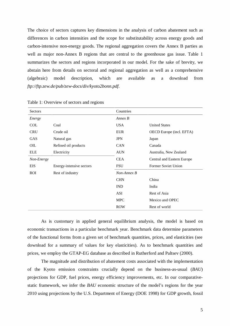
The choice of sectors captures key dimensions in the analysis of carbon abatement such as

differences in carbon intensities and the scope for substitutability across energy goods and

carbon-intensive non-energy goods. The regional aggregation covers the Annex B parties as

well as major non-Annex B regions that are central to the greenhouse gas issue. Table 1

summarizes the sectors and regions incorporated in our model. For the sake of brevity, we

abstain here from details on sectoral and regional aggregation as well as a comprehensive

(algebraic) model description, which are available as a download from

ftp://ftp.zew.de/pub/zew-docs/div/kyoto2bonn.pdf.

Table 1: Overview of sectors and regions

Sectors Countries

Energy Annex B

COL Coal USA United States

CRU Crude oil EUR OECD Europe (incl. EFTA)

GAS Natural gas JPN Japan

OIL Refined oil products CAN Canada

ELE Electricity AUN Australia, New Zealand

Non-Energy CEA Central and Eastern Europe

EIS Energy-intensive sectors FSU Former Soviet Union

ROI Rest of industry Non-Annex B

CHN China

IND India

ASI Rest of Asia

MPC Mexico and OPEC

ROW Rest of world

As is customary in applied general equilibrium analysis, the model is based on

economic transactions in a particular benchmark year. Benchmark data determine parameters

of the functional forms from a given set of benchmark quantities, prices, and elasticities (see

download for a summary of values for key elasticities). As to benchmark quantities and

prices, we employ the GTAP-EG database as described in Rutherford and Paltsev (2000).

The magnitude and distribution of abatement costs associated with the implementation

of the Kyoto emission constraints crucially depend on the business-as-usual (BAU)

projections for GDP, fuel prices, energy efficiency improvements, etc. In our comparative-

static framework, we infer the BAU economic structure of the model’s regions for the year

2010 using projections by the U.S. Department of Energy (DOE 1998) for GDP growth, fossil

6

fuel production, and future energy prices. We incorporate autonomous energy efficiency

improvement factors which scale energy demand functions to match the exogenous DOE

emission forecasts. The simulation results for emission abatement scenarios reported in

section 4 are measured with respect to the BAU situation in 2010.

3. Policy Scenarios

The set of scenarios reflects alternative options for implementing the Kyoto Protocol along

three important dimensions of climate change policy, which are laid out in the following.

A. Reduction Requirements

The Kyoto Protocol fixes GHG emission limits for industrialized countries as listed in Annex

B of the Protocol. In our simulations we consider two different schemes of emission reduction

targets:

OLD Option OLD considers a reduction target of 5.2 % on average for industrialized

countries which the Kyoto Protocol originally aspired to.

NEW Option NEW accounts for carbon dioxide sinks as agreed on in Bonn and

confirmed in Marrakesh: Countries can offset some of the CO2 stored in their

forests and farmlands to meet their emission limits.

Table 2 lists the original reduction targets (OLD) and revised targets (NEW) for Annex

B countries accounting for potential sink credits (see also Appendix C in download).

Table 2: Original Kyoto reduction targets (OLD) and Bonn updates with sink credits (NEW)

OLD Commitmenta

(% of 1990 base year GHG emissions)

NEW Commitmentb


USA 93.0 96.8

EUR 92.2 94.8

JPN 94.0 99.2

CAN 94.0 107.9

AUN 106.8 110.2

CEA 92.9 96.1

FSU 100.0 107.6

a UNFCCC (1997)b Estimates by the European Commission (Nemry 2001)

7

Credits are composed of sinks from forest management, sinks from agricultural

activities and sinks in CDM. Due to the lack of appropriate data, we assume that there are no

costs to earning credits such that the overall economic gains and the relaxation of emission

constraints through sink credits must be seen as an upper bound.

B. Scope of Emissions Trading

The Bonn compromise does not set clear limits on the magnitude of international emissions

trading that the industrialized countries could engage in to achieve their targets. The scope of

permissible emissions trading has been a major point of disagreement between the U.S. and

the EU. The EU wanted nations to make at least half of their emissions cuts within their own

borders, whereas the U.S. wanted no limit on the purchase of emission rights from other

countries.

In our simulations, we capture extreme points on the extent to which countries can

meet their specific emission reduction commitment by abatement abroad (so-called where-

flexibility). Unrestricted where-flexibility among Annex B countries should be considered the

relevant policy option emerging from the Bonn compromise:

NTR Annex B countries are restricted to domestic action for meeting their emission

reduction commitment.

TRD There is unrestricted emission trading between Annex B countries, which assures

equalization of marginal abatement costs but also allows countries to sell off

abundant emission rights (hot air) that they would not have required in the NTR

case.

C. Participation of the U.S.

In March 2001, the new U.S. administration under President G. W. Bush declared with

respect to the Kyoto Protocol that "we have no interest in implementing this treaty." Since

then, the EU has tried hard to persuade the U.S. to rejoin the Kyoto Process - so far, however,

without success. Even the Bonn compromise could not appease the U.S., although it resolves

several of the demands the U.S. had raised in the past - particularly concerning sink credits

and international permit trading. It is nonetheless important for the international climate

policy process to investigate how the economic and environmental impacts of the Kyoto

Protocol change depending on the involvement of the U.S. We therefore take into account two

options which deliver a useful angle of comparison:

USin Option USin assumes that the U.S. will keep with its Kyoto commitment.

8

USout Option USout reflects the current situation of U.S. climate policy in assuming that

the USA will not be part of the Kyoto Protocol.

Table 3 summarizes the set of core scenarios that result from the combination of

policy options as laid out above.

Table 3: Overview of scenarios

Emission Reduction Emissions Trading U.S. Participation

OLD NEW NTR TRD USin USout

USin_NTR_OLD X X X

USout_NTR_OLD X X X

USin_TRD_OLD X X X

USout_TRD_OLD X X X

USin_NTR_NEW X X X

USout_NTR_NEW X X X

USin_TRD_NEW X X X

USout_TRD_NEW X X X

4. Simulation Results

The economic and environmental impacts induced by alternative scenarios for the

implementation of the Kyoto Protocol are measured with respect to a BAU reference point in

2010 without emission abatement policies. When we report results for the aggregate of Annex

B (Label: ANNEXB) or non-Annex B (Label: NONAB) in the Tables below, we assume that

the U.S. only forms part of Annex B or OECD if it sticks to its Kyoto commitment (USin

scenarios), otherwise the aggregate of non-Annex B takes the U.S. into account. It should be

noted that scenarios USin_NTR_OLD and USin_TRD_OLD reflect the policy settings that

have been studied extensively in the literature on the economic impacts of the Kyoto Protocol.

These simulations are repeated here to provide a consistent basis of comparison with the new

scenarios capturing the implications of U.S. withdrawal and sink credits. All the results for

USin_NTR_OLD and USin_TRD_OLD are in line with the quantitative estimates reported in

previous studies (see e.g. Weyant 1999).

A. Compliance of the U.S. - No Emissions Trading

We start discussion of simulation results for the scenarios USin_NTR_OLD and

USin_NTR_NEW where the U.S. meets its Kyoto targets (in the OLD or NEW version), and

9

reduction commitments are met exclusively by domestic action of Annex B countries. The

potential economic impacts reported in Table 4 indicate why the U.S. has withdrawn from the

Protocol and why JPN, CAN as well as AUN have pushed hard for the relaxation of their

Kyoto targets via the accounting of sinks and unlimited Annex B emissions trading.

Emission constraints as originally mandated under the Kyoto Protocol induce non-

negligible adjustment costs to OECD countries. The reason is that emission targets, which are

stated with respect to 1990, translate into much higher effective carbon reduction requirements

with respect to business-as-usual emission levels during the Kyoto budget period between

2008-2012. Without “where”-flexibility, the effective emission constraints require substantial

changes in the production and consumption patterns of OECD countries towards less carbon-

intensity which induces a loss of productivity and real income (consumption). The marginal

abatement costs per ton of carbon under USin_NTR_OLD are as follows: USA 170 USD,

EUR 168 USD, JPN 394 USD, CAN 193 USD, and AUN 85 USD.8 Abatement in OECD

countries produces significant spillovers to non-abating regions through induced changes in

international prices, i.e. the terms of trade.9

Most important are changes on international fuel markets for crude oil, gas and coal.

The cutback in global demand for fossil fuels implies a significant drop of their prices

providing economic gains to fossil fuel importers and losses to fossil fuel exporters. These

fossil fuel market effects explain most of the impacts for non-abating countries. The economic

implications of international price changes on non-energy markets are more complex. Higher

energy costs raise the prices of non-energy goods (particularly energy-intensive goods)

produced in abating countries. Countries that import these goods suffer from higher prices to

the extent that they can not substitute away towards cheaper imports of non-abating countries.

The ease of substitution not only determines the implicit burden shifting via non-energy

exports from abating countries but also the extent to which non-abating countries achieve a

competitive advantage vis-à-vis abating exporters. The gain in market shares due to

substitution effects may be partially offset by an opposite scale effect: Due to reduced

economic activity and income, import demand by the group of abating countries (here: Annex

8 From a single country perspective, there is a straightforward monotonous correlation between the

level of cutback, the induced marginal abatement cost and the associated infra-marginal consumptionloss. However, these relationships do not necessarily carry over for the comparison across countries,since differences in energy prices, energy intensities, substitution elasticities, etc. across countries alsomatter.9 See Babiker, Reilly and Jacoby (2000) or Böhringer and Rutherford (2002) for an elaboratediscussion of terms-of-trade effects from GHG abatement policies.

10

B) declines, and this exerts a downward pressure on the export prices of non-abating

countries.

Less stringent emission targets as adopted in Bonn reduce consumption losses of the

Annex B group by more than 25 % - the adjustment costs to OECD countries, however,

remain substantial.10

With respect to environmental effectiveness, domestic abatement by Annex B

countries implies a global reduction of carbon emission by 9 % (OLD) or 7.9 % (NEW)

compared to BAU. Leakage, which is mainly caused by increased fossil fuel demand of non-

abating countries and shifts in the pattern of energy-intensive trade, amounts to more than 10

%.11

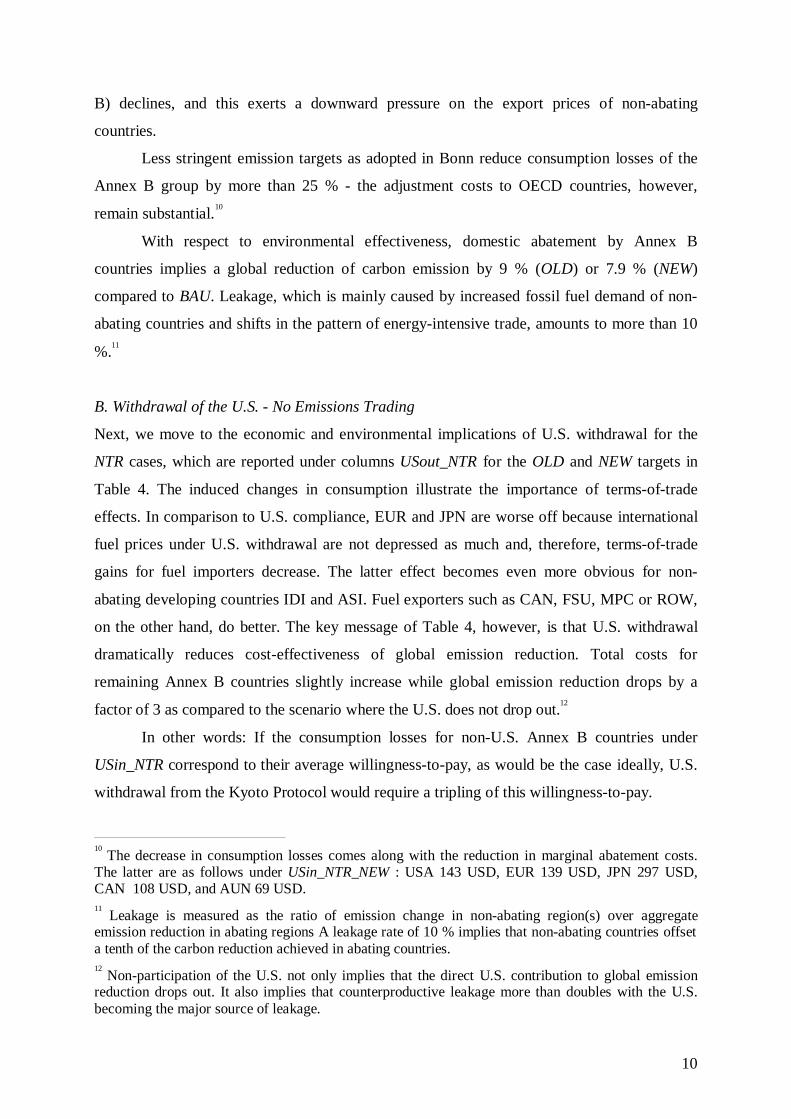
B. Withdrawal of the U.S. - No Emissions Trading

Next, we move to the economic and environmental implications of U.S. withdrawal for the

NTR cases, which are reported under columns USout_NTR for the OLD and NEW targets in

Table 4. The induced changes in consumption illustrate the importance of terms-of-trade

effects. In comparison to U.S. compliance, EUR and JPN are worse off because international

fuel prices under U.S. withdrawal are not depressed as much and, therefore, terms-of-trade

gains for fuel importers decrease. The latter effect becomes even more obvious for non-

abating developing countries IDI and ASI. Fuel exporters such as CAN, FSU, MPC or ROW,

on the other hand, do better. The key message of Table 4, however, is that U.S. withdrawal

dramatically reduces cost-effectiveness of global emission reduction. Total costs for

remaining Annex B countries slightly increase while global emission reduction drops by a

factor of 3 as compared to the scenario where the U.S. does not drop out.12

In other words: If the consumption losses for non-U.S. Annex B countries under

USin_NTR correspond to their average willingness-to-pay, as would be the case ideally, U.S.

withdrawal from the Kyoto Protocol would require a tripling of this willingness-to-pay.

10

The decrease in consumption losses comes along with the reduction in marginal abatement costs.The latter are as follows under USin_NTR_NEW : USA 143 USD, EUR 139 USD, JPN 297 USD,CAN 108 USD, and AUN 69 USD.11

Leakage is measured as the ratio of emission change in non-abating region(s) over aggregateemission reduction in abating regions A leakage rate of 10 % implies that non-abating countries offseta tenth of the carbon reduction achieved in abating countries.12

Non-participation of the U.S. not only implies that the direct U.S. contribution to global emissionreduction drops out. It also implies that counterproductive leakage more than doubles with the U.S.becoming the major source of leakage.

11

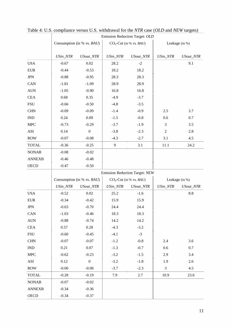
Table 4: U.S. compliance versus U.S. withdrawal for the NTR case (OLD and NEW targets)Emission Reduction Target: OLD

Consumption (in % vs. BAU) CO2-Cut (in % vs. BAU) Leakage (in %)

USin_NTR USout_NTR USin_NTR USout_NTR USin_NTR USout_NTR

USA -0.67 0.02 28.2 -2 9.1

EUR -0.44 -0.53 18.2 18.2

JPN -0.88 -0.95 28.3 28.3

CAN -1.81 -1.09 28.9 28.9

AUN -1.05 -0.90 16.8 16.8

CEA 0.68 0.35 -4.9 -3.7

FSU -0.66 -0.50 -4.8 -3.5

CHN -0.09 -0.09 -1.4 -0.9 2.5 3.7

IND 0.24 0.09 -1.5 -0.8 0.6 0.7

MPC -0.73 -0.29 -3.7 -1.9 3 3.5

ASI 0.14 0 -3.8 -2.3 2 2.8

ROW -0.07 -0.08 -4.3 -2.7 3.1 4.5

TOTAL -0.36 -0.25 9 3.1 11.1 24.2

NONAB -0.08 -0.02

ANNEXB -0.46 -0.48

OECD -0.47 -0.50

Emission Reduction Target: NEW

Consumption (in % vs. BAU) CO2-Cut (in % vs. BAU) Leakage (in %)

USin_NTR USout_NTR USin_NTR USout_NTR USin_NTR USout_NTR

USA -0.52 0.02 25.2 -1.6 8.8

EUR -0.34 -0.42 15.9 15.9

JPN -0.63 -0.70 24.4 24.4

CAN -1.03 -0.46 18.3 18.3

AUN -0.88 -0.74 14.2 14.2

CEA 0.57 0.28 -4.3 -3.2

FSU -0.60 -0.45 -4.1 -3

CHN -0.07 -0.07 -1.2 -0.8 2.4 3.6

IND 0.21 0.07 -1.3 -0.7 0.6 0.7

MPC -0.62 -0.23 -3.2 -1.5 2.9 3.4

ASI 0.12 0 -3.2 -1.8 1.9 2.6

ROW -0.06 -0.06 -3.7 -2.3 3 4.5

TOTAL -0.28 -0.19 7.9 2.7 10.9 23.6

NONAB -0.07 -0.02

ANNEXB -0.34 -0.36

OECD -0.34 -0.37

12

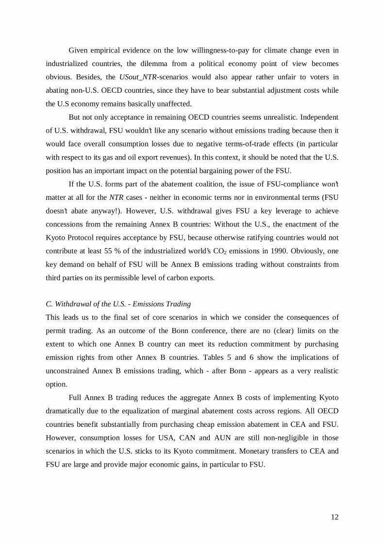
Given empirical evidence on the low willingness-to-pay for climate change even in

industrialized countries, the dilemma from a political economy point of view becomes

obvious. Besides, the USout_NTR-scenarios would also appear rather unfair to voters in

abating non-U.S. OECD countries, since they have to bear substantial adjustment costs while

the U.S economy remains basically unaffected.

But not only acceptance in remaining OECD countries seems unrealistic. Independent

of U.S. withdrawal, FSU wouldn’t like any scenario without emissions trading because then it

would face overall consumption losses due to negative terms-of-trade effects (in particular

with respect to its gas and oil export revenues). In this context, it should be noted that the U.S.

position has an important impact on the potential bargaining power of the FSU.

If the U.S. forms part of the abatement coalition, the issue of FSU-compliance won’t

matter at all for the NTR cases - neither in economic terms nor in environmental terms (FSU

doesn’t abate anyway!). However, U.S. withdrawal gives FSU a key leverage to achieve

concessions from the remaining Annex B countries: Without the U.S., the enactment of the

Kyoto Protocol requires acceptance by FSU, because otherwise ratifying countries would not

contribute at least 55 % of the industrialized world’s CO2 emissions in 1990. Obviously, one

key demand on behalf of FSU will be Annex B emissions trading without constraints from

third parties on its permissible level of carbon exports.

C. Withdrawal of the U.S. - Emissions Trading

This leads us to the final set of core scenarios in which we consider the consequences of

permit trading. As an outcome of the Bonn conference, there are no (clear) limits on the

extent to which one Annex B country can meet its reduction commitment by purchasing

emission rights from other Annex B countries. Tables 5 and 6 show the implications of

unconstrained Annex B emissions trading, which - after Bonn - appears as a very realistic

option.

Full Annex B trading reduces the aggregate Annex B costs of implementing Kyoto

dramatically due to the equalization of marginal abatement costs across regions. All OECD

countries benefit substantially from purchasing cheap emission abatement in CEA and FSU.

However, consumption losses for USA, CAN and AUN are still non-negligible in those

scenarios in which the U.S. sticks to its Kyoto commitment. Monetary transfers to CEA and

FSU are large and provide major economic gains, in particular to FSU.

13

Table 5: Impacts of U.S. withdrawal for the TRD case and OLD targets

Consumption (in % vs. BAU) Marginal Abatement Costs (USD/ton C)

USin_NTR USin_TRD USout_TRD USin_NTR USin_TRD USout_TRD

USA -0.67 -0.40 0 170 61

EUR -0.44 -0.16 -0.03 168 61 7

JPN -0.88 -0.15 -0.03 394 61 7

CAN -1.81 -0.92 -0.10 193 61 7

AUN -1.05 -0.82 -0.11 85 61 7

CEA 0.68 1.40 0.09 0 61 7

FSU -0.66 7.67 0.81 0 61 7

CHN -0.09 0.03 0

IND 0.24 0.16 0.01

MPC -0.73 -0.45 -0.04

ASI 0.14 0.15 0.01

ROW -0.07 -0.01 0

TOTAL -0.36 -0.06 0

NONAB -0.08 -0.03 0

ANNEXB -0.46 -0.07 0

OECD -0.47 -0.19 -0.02

CO2-Cut (in % vs. BAU) Leakage (in %)


USA 28.2 13.3 -0.2 0.8

EUR 18.2 7.5 1.1

JPN 28.3 7.4 1.2

CAN 28.9 12.4 2.2

AUN 16.8 13.4 2.1

CEA -4.9 17.9 2.8

FSU -4.8 16.7 2.6

CHN -1.4 -1.3 -0.2 2.5 2.2 0.6

IND -1.5 -1.1 -0.1 0.6 0.4 0.1

MPC -3.7 -2.8 -0.3 3 2.3 0.5

ASI -3.8 -2.5 -0.3 2 1.4 0.3

ROW -4.3 -2.7 -0.3 3.1 1.9 0.5

TOTAL 9 5.8 0.5 11.1 8.2 2.8

14

Table 6: Impacts of U.S. withdrawal for the TRD case and NEW targets

Consumption (in % vs. BAU) Marginal Abatement Costs (USD/ton C)


USA -0.52 -0.24 0 143 37

EUR -0.34 -0.08 0 139 37 0

JPN -0.63 -0.08 0 297 37 0

CAN -1.03 -0.45 0 108 37 0

AUN -0.88 -0.53 0 69 37 0

CEA 0.57 0.87 0 0 37 0

FSU -0.60 5.23 0 0 37 0

CHN -0.07 0.02 0

IND 0.21 0.10 0

MPC -0.62 -0.29 0

ASI 0.12 0.09 0

ROW -0.06 -0.01 0

TOTAL -0.28 -0.03 0

NONAB -0.07 -0.02 0

ANNEXB -0.34 -0.03 0

OECD -0.34 -0.11 0

CO2-Cut (in % vs. BAU) Leakage (in %)


USA 25.2 8.6 0 0

EUR 15.9 4.8 0

JPN 24.4 4.8 0

CAN 18.3 8 0

AUN 14.2 8.8 0

CEA -4.3 12 0

FSU -4.1 11.1 0

CHN -1.2 -0.8 0 2.4 1.7 0

IND -1.3 -0.7 0 0.6 0.3 0

MPC -3.2 -1.8 0 2.9 1.6 0

ASI -3.2 -1.6 0 1.9 1 0

ROW -3.7 -1.7 0 3 1.5 0

TOTAL 7.9 3.8 0 10.9 6 0

As expected, adoption of the less stringent emission reduction targets (NEW) not only

reduces the burden to OECD countries but also the benefits to CEA and FSU from permit

trading: The decline in abatement demand of OECD countries drives down the price of

15

tradable permits. Trade in emission rights reduces global leakage. However, global emission

reduction under U.S. compliance drops by one third for the original Kyoto targets (OLD) and

by one half for the revised Kyoto targets (NEW) as a consequence of hot air. This negative

impact on global emission reduction should not obscure the fact that global emissions fall

noticeably and average costs per emission reduction for abating OECD countries are much

more favorable as compared to the cases without emission trading (USin_NTR and, in

particular, USout_NTR).

U.S. withdrawal, joint with emissions trading between remaining Annex B countries,

implies negligible costs for meeting the OLD Kyoto targets and zero costs for meeting the

NEW Kyoto targets. Since the U.S., as the world largest potential buyer of emission rights,

withdraws from the permit market, the price of emission permits falls close to zero in the

OLD case. With relaxed Kyoto targets (NEW), the permit price even hits zero, as the demand

of remaining Annex B countries is small relative to the supply of surplus emission rights from

FSU and CEA. While U.S. withdrawal and unconstrained Annex B emissions trading sounds

like good news from the aggregate cost side, the environmental effectiveness is more or less

zero. In other words, Kyoto comes at no costs because the world economy and its emissions

develop as under business-as-usual.

5. Sensitivity AnalysisThe preceding section provided a comprehensive assessment of U.S. withdrawal, sink credits,

and emissions trading under central case assumptions. We have performed a sensitivity

analysis with respect to changes in several key assumptions: market structure of emissions

trading, scope of emissions trading, and ease of substitution among traded goods. In this

section, we summarize the implications of changes in underlying key assumptions. For the

sake of compactness, all the numerical results are based on the revised Kyoto targets. While

the magnitude of quantitative results can be altered as a consequence of model assumptions,

we have found that all of our key insights remain robust. As for the previous Tables, it should

be kept in mind that that the U.S. only forms part of Annex B or OECD if it sticks to its

Kyoto commitment (USin scenarios), otherwise the aggregate of non-Annex B takes the U.S.

into account ((USout scenarios)).

A. Monopolistic Permit Supply

Competitive behavior of FSU and CEA on the permit market may seem somewhat

implausible for the case in which the international permit price falls to zero, and emission

16

sales therefore do not create any revenue. What will happen if these countries behave as

monopolists restricting their supply in order to drive up the international carbon price? As a

shortcut, we mimic such a behavior by imposing caps on emission right exports from FSU

and CEA where rents from export quotas accrue to FSU and CEA respectively. Concretely,

we assume that export quotas for FSU and CEA will be 0 %, 20 %, 40%, 60 %, 80 %, and

100 % of the difference between their business-as-usual emissions and their emission

entitlements after the Bonn updates.13 Table 7 summarizes results for non-compliance of the

U.S., and otherwise unrestricted intra-OECD emissions trading. As export quotas between 80

% and 100 % imply an excess supply of permits on international markets, i.e. no change vis-

à-vis BAU, we have omitted the respective columns.

We have also listed the results for the scenario USout_NTR_NEW to accommodate the

direct comparison with the NTR case. Column "0" of Table 7 captures a situation in which

FSU and CEA will not export any emission rights but only intra-OECD emissions trading will

take place. The latter cuts down compliance costs for the OECD by 13.5 % without loss of

environmental effectiveness as compared to the no-emission-trading case

(USout_NTR_NEW).

Table 7: Export quotas on hot air from FSU and CEA

USout_NTR_NEW 0 20 40 60

Consumption (in % vs. BAU)

CEA 0.28 0.28 0.45 0.42 0.25

FSU -0.45 -0.40 2.10 2.60 1.70

TOTAL -0.19 -0.16 -0.10 -0.05 -0.02

NONAB -0.02 -0.01 -0.01 -0.01 0

ANNEXB -0.36 -0.31 -0.18 -0.10 -0.04

OECD -0.37 -0.32 -0.24 -0.16 -0.08

CO2-Cut (in % vs. BAU)

TOTAL 2.7 2.7 2 1.3 0.6

Leakagea (in %)

TOTAL 24 24 17 11 5

a Ratio of emission change in non-abating region over aggregate emission reduction in abating regions

13

Note that the case "100%", where FSU and CEA sell off total hot air, coincides with the scenarioUSout_TRD_NEW.

17

When FSU and CEA sell hot air, the international price of carbon permits as well as

total OECD compliance costs fall towards larger amounts of hot air exports. The numerical

results indicate that FSU would aim at restricting permits sales at 40 % of hot air in order to

maximize consumption.14 In this case, global emission reduction as compared to BAU drops to

roughly 1 %. Obviously, leakage rates decline with the increase in hot air sales as the latter

relaxes the overall carbon emission constraint for abating Annex B countries.

Table 7 illustrates the potential trade-offs between environmental effectiveness and

total costs of OECD compliance on the one hand, as well as burden sharing between OECD

and FSU/CEA on the other hand.

B. EU Cap Proposal

In order to mitigate hot air, the EU called for restrictive ceilings on the amount of tradable

emissions. According to the cap proposal by the EU Council of Environment (Baron et al.

1999), purchases or sales of emissions by Annex B countries may not exceed 5 percent of the

weighted average of base year emissions and the assigned Kyoto emission budget. Table 8

reports the implications for economic costs and environmental effectiveness (columns:

"USin_EU", "USout_EU").

Table 8: Implications of EU cap proposal

USin_NTR USin_EU USin_TRD USout_NTR USout_EU USout_TRD


USA -0.52 -0.51 -0.24 0.02 0.01 0

TOTAL -0.28 -0.22 -0.03 -0.19 -0.12 0

NONAB -0.07 -0.06 -0.02 -0.02 -0.01 0

ANNEXB -0.34 -0.28 -0.03 -0.36 -0.24 0

OECD -0.34 -0.32 -0.11 -0.37 -0.28 0


TOTAL 7.9 7.3 3.8 2.7 2.2 0

Leakage (in %)

TOTAL 10.9 9.9 6 23.6 19.3 0

14

Note that CEA prefers a slightly more restrictive export quota regime because the foregone revenuesfrom permit sales would be more than offset from terms-of-trade gains on fossil fuel markets due tothe larger fall in international fuel prices.

18

In comparison with unrestricted emissions trading, the EU cap proposal reduces hot air

to a large extent. However, the restrictive ceilings also imply a substantial loss in overall

efficiency since marginal abatement costs will differ substantially between various regions

(causing also higher leakage rates as compared to the TRD case). In particular, the EU cap

proposal provides very small efficiency gains to the U.S. vis-à-vis the NTR case which

explains the stiff U.S. resistance to this plan during the climate negotiations. In almost the

same manner as under NTR, U.S. withdrawal makes global abatement much more expensive

for non-U.S. OECD countries under cost-effectiveness considerations.

C. Trade Elasticities

We represent trade in goods with an Armington structure. Imports are imperfect

substitutes for domestically produced goods. The elasticity of substitution between imports

and domestically produced goods, referred to as the Armington elasticity, measures how

easily imports can substitute for domestic goods. In the sensitivity analysis, we vary the

values of Armington elasticities to quantify the induced changes in trade impacts of carbon

abatement policies.

In our central case, the elasticity of substitution between the domestic good and the

import aggregate is set equal to 4.0, and the elasticity of imports from different regions within

the import aggregate is set equal to 8.0. In the sensitivity analysis, we either halve (low case)

or double (high case) these values.

While the change in elasticities has only a negligible impact on total adjustment

costs15, the ease of substitution affects the distribution of costs via changes in regions' primary

abatement costs and secondary terms-of-trade effects. In the absence of terms-of-trade effects,

the cost of carbon abatement moves inversely with trade elasticities because countries can

more easily substitute away from carbon-intensive inputs into production and consumption.

On the other hand, the trade elasticity determines the extent to which domestic abatement

costs can be passed further to trading partners. With lower elasticities, a country importing

carbon-intensive goods from a trading partner with high marginal abatement costs is less able

to substitute away from the more expensive imports to the cheaper domestically produced

goods. Our sensitivity analysis indicates that abating countries (ANNEXB) are worse off for

higher trade elasticities indicating their reduced scope for effective tax burden shifting. On the

15

In general, total welfare costs of emissions constraints on the global economy decline towards highertrade elasticities.

19

other hand, non-abating countries (NONAB) face less adverse spillover impacts towards

higher elasticities because (i) they can more readily substitute away from expensive energy-

intensive goods of abating countries, and (ii) they can take greater advantage of their lower

domestic production costs in competing against the abating countries. With respect to

environmental spillovers, higher trade elasticities enforce the adverse impacts on energy-

intensive industries in abating regions which leads to an increase in the global leakage rate.

Table 9: Implications of alternative Armington elasticities

Armington elasticities: low

USin_NTR USin_TRD USout_NTR USout_TRD


TOTAL -0.28 -0.04 -0.19 0

NONAB -0.13 -0.05 -0.03 0

ANNEXB -0.33 -0.03 -0.35 0

OECD -0.33 -0.12 -0.36 0


TOTAL 8.3 4.2 3 0

Leakage (in %)

TOTAL 8.4 4.5 19.7 0

Armington elasticities: high

USin_NTR USin_TRD USout_NTR USout_TRD


TOTAL -0.28 -0.02 -0.19 0

NONAB -0.05 -0.01 -0.01 0

ANNEXB -0.35 -0.03 -0.37 0

OECD -0.35 -0.10 -0.39 0


TOTAL 7.4 3.4 2.4 0

Leakage (in %)

TOTAL 15.3 7.8 29.7 0

6. Conclusions

In this paper, we investigated different scenarios for implementing the Kyoto Protocol,

combining alternative options along three important policy dimensions: U.S. compliance

versus U.S. withdrawal, domestic action versus unrestricted Annex B emissions trading, and

the original Kyoto targets versus the relaxed targets of Bonn.

20

Our results clearly indicate that U.S. withdrawal from the Protocol implies a dramatic

reduction in environmental effectiveness. If emission trading among remaining Annex B

countries becomes more or less unrestricted, which seems to be rather likely after the Bonn

outcome, the reduction of global carbon emissions as compared to BAU will fall to zero. The

reason is that supply of surplus emission rights from Russia, Ukraine, and Eastern Europe is

large relative to the demand from OECD countries other than the U.S., driving down the

permit price close to zero (if Kyoto targets had not been relaxed for sink credits) or to zero (if

Kyoto targets are updated with sink credits).

If remaining OECD countries would opt for strictly domestic action in order to prevent

hot air, global carbon emissions could be reduced by 2.7 % (with sink credits) or 3.1 %

(without sink credits). However, the global emission cutback would then only amount to

roughly a third of the value that could be achieved for U.S. compliance while remaining

OECD countries would suffer more or less the same non-negligible adjustment costs. Implicit

willingness-to-pay, thus, would have to triple in these countries. Such a policy appears rather

unacceptable to citizens in non-U.S. OECD countries - not only with regard to overall cost-

effectiveness but also with respect to fairness considerations. The same reasoning applies to

the case there non-U.S. OECD countries would adopt the EU cap proposal instead of strictly

domestic action.

If Russia, Ukraine, and Eastern Europe restrict the supply of hot air to drive up the

price of permits, this would prevent environmental effectiveness from falling to zero in the

case of U.S. withdrawal. Global emission reduction under monopolistic permit supply will

nevertheless amount to only 1 % as compared to business-as-usual.

Policy makers have welcomed the outcome of the Bonn climate negotiations as a

decisive breakthrough in international climate politics. The environmental effects can not be

the reason for celebration: Sink credits, hot air through emissions trading and, in particular,

the continued U.S. withdrawal will make Kyoto ineffective in environmental terms.

However, it can be argued that - even without any effective emission cutback - the

ratification of Kyoto is crucial for the further policy process of climate protection. Failure

might have thrown back the efforts to climate protection by several years. Hopes remain that

the U.S. might rejoin the Protocol under the new conditions. Compliance costs to the U.S.

economy seem rather moderate, which could enhance the domestic U.S. political pressure in

favor of coordinated international abatement. Starting from a ratified Kyoto Protocol, it may

be also easier to achieve effective GHG emission reduction in the second commitment period

of the Kyoto Protocol after 2012.

21

There are some caveats to our analysis which may be addressed in future research

once the relevant information and data is available: First, we do not cover a further

commitment period after 2012 which might influence behavior in the first commitment (e.g.

through banking of emission permits). Second, we assume for the case of U.S. withdrawal

that the U.S. will not undertake any domestic policies to cut GHG emissions. Third, no other

greenhouse gases besides CO2 are incorporated in our analysis, i.e., we apply GHG emission

reduction targets to carbon dioxide only, which is the most important GHG among

industrialized countries.

References

Baron, R., M. Bosi, A. Lanza and J. Pershing (1999), A Preliminary Analysis of the EU

Proposals on the Kyoto Mechanisms, Energy and Environment Division, International

Energy Agency, http://www.iea.org/new/releases/1999/eurpro/eurlong.html

Bernstein, P., D. Montgomery, T. F. Rutherford and G. Yang (1999), Effects of Restrictions

on International Permit Trading: The MS-MRT Model, The Energy Journal – Special

Issue, 221-257.

Böhringer, C. (2000), Cooling Down Hot Air - A Global CGE Analysis of Post-Kyoto Carbon

Abatement Strategies, Energy Policy 28, 779-789.

Böhringer, C. and T. F. Rutherford (2002), Carbon Abatement and International Spillovers,

Environmental and Resource Economics (forthcoming).

Bollen, J., A. Gielen and H. Timmer (1999), Clubs, Ceilings and CDM – Macroeconomics of

Compliance with the Kyoto Protocol, The Energy Journal – Special Issue, 177-206.

Criqui, P., S. Mima and L. Viguier (1999), Marginal abatement costs of CO2 emission

reductions, geographical flexibility and concrete ceilings: an assessment using the

POLES model, Energy Policy 27, 585-602.

DOE (1998), Department of Energy, Annual Energy Outlook (AEO 1998), Energy

Information Administration, http://www.eia.doe.gov

Ellerman, A.D. and I. S. Wing (2000), Supplementarity: An Invitation for Monopsony, The

Energy Journal 21 (4), 29-59.

Hagem, C. and B. Holtsmark, From small to insignificant: Climate impact of the Kyoto

Protocol with and without US, CICERO Policy Note 2001:1, htttp://www.cicero.uio.no

Nemry, F. (2001), LULUCF39 v4 - Quantitative implications of the decision -/CP.7 on

LULUCF, Personal Communication.

22

Paltsev, S.V. (2000), The Kyoto Protocol: Hot Air for Russia?, University of Colorado,

Working Paper 00-9, http://debreu.colorado.edu/projects/sergey_hotair.pdf

Paltsev, S.V. (2001), The Kyoto Protocol: Regional and Sectoral Contributions to the Carbon

Leakage, The Energy Journal 22 (4), 53-79.

Rose, A., and B. Stevens (2001), An Economic Analysis of Flexible Permit Trading in the Kyoto

Protocol, International Environmental Agreements 1, 219-42.

Rutherford, T.F. and S.V. Paltsev (2000), GTAP-Energy in GAMS, University of Colorado,

Working Paper 00-2, http://debreu.colorado.edu/download/gtap-eg.pdf

UNFCCC (1997), United Nations Framework Convention on Climate Change, Kyoto

Protocol to the United Nations Framework Convention on Climate Change,

FCCC/CP/L.7/Add.1, Kyoto.

Weyant, J. (ed) (1999), The Costs of the Kyoto Protocol: A Multi-Model Evaluation, The

Energy Journal, Special Issue.

23

Appendix A: Detailed Algebraic Model Description

This section outlines the main characteristics of a generic static general equilibrium model of

the world economy designed for the medium-run economic analysis of carbon abatement

constraints. It is a well-known Arrow-Debreu model that concerns the interaction of

consumers and producers in markets. Consumers in the model have a primary exogenous

endowment of the commodities and a set of preferences giving demand functions for each

commodity. The demands depend on all prices; they are continuous and non-negative,

homogenous of degree zero in factor prices and satisfy Walras’ Law, i.e. the total value of

consumer expenditure equals consumer income at any set of prices. Market demands are the

sum of final and intermediate demands. Producers maximize profits given a constant returns

to scale production technology. Because of the homogeneity of degree zero of the demand

functions and the linear homogeneity of the profit functions in prices, only relative prices

matter in such a model. Two classes of conditions characterize the competitive equilibrium in

the model: market clearance conditions and zero profit conditions. In equilibrium, price levels

and production levels in each industry are such that market demand equals market supply for

each commodity. Profit maximization under a constant returns to scale technology implies

that no activity does any better than break even at equilibrium prices. The model is a system

of simultaneous, non-linear equations with the number of equations equal to the number of

variables.

A.1 Production

Within each region (indexed by the subscript r), each producing sector (indexed

interchangeable by i and j) is represented by a single-output producing firm which chooses

input and output quantities in order to maximize profits. Firm behavior can be construed as a

two-stage procedure in which the firm selects the optimal quantities of primary factors k

(indexed by f) and intermediate inputs x from other sectors in order to minimize production

costs given input prices and some production level Y with

Y = ϕ (k,x) the production functions. The second stage, given an exogenous output price, is

the selection of the output level Y to maximize profits. The firm’s problem is then:

( ) ( ), ,

, , . . ,jir jir fir

ir ir ir ir jr fr ir ir ir jir firy x k

Max p Y C p w Y s t Y x kϕΠ = ⋅ − = [1]

where Π denotes the profit functions, C the cost functions which relate the minimum

possible total costs of producing Y to the positive input prices, technology parameters, and the

output quantity Y, and p and w are the prices for goods and factors, respectively.

24

Production of each good takes place according to constant elasticity of substitution

(CES) production functions, which exhibit constant returns to scale. Therefore, the output

price equals the per-unit cost in each sector, and firms make zero profits in equilibrium

(Euler’s Theorem). Profit maximization under constant returns to scale implies the

equilibrium condition:

( , ) 0ir ir ir jr frp c p wπ = − = (zero profit condition) [2]

where c and π are the unit cost and profit functions, respectively.

Demand functions for goods and factors can be derived by Shepard’s Lemma. It

suggests that the first-order differentiation of the cost function with respect to an input price

yields the cost-minimizing demand function for the corresponding input. Hence, the

intermediate demand for good j in sector i is:

ir irjir ir

jr jr

C cx Y

p p

∂ ∂= = ⋅

∂ ∂ [3]

and the demand for factor f in sector i is:

ir irfir ir

fr fr

C ck Y

w w

∂ ∂= = ⋅

∂ ∂ [4]

The profit functions possess a corresponding derivative property (Hotelling’s Lemma):

ir irjir ir

jr jrx Y

p p

π∂ Π ∂= = ⋅

∂ ∂ and ir ir

fir irfr fr

k Yw w

π∂ Π ∂= = ⋅

∂ ∂ [5]

The variable, price dependent input coefficients, which appear subsequently in the

market clearance conditions, are thus:

x ir irjir

jr jr

ca

p p

π∂ ∂= =

∂ ∂ and k ir ir

firfr fr

ca

w w

π∂ ∂= =

∂ ∂ [6]

25

The model captures the production of commodities by aggregate, hierarchical (or

nested) constant elasticity of substitution (CES) production functions that characterize the

technology through substitution possibilities between capital, labor, energy and material (non-

energy) intermediate inputs (KLEM). Two types of production functions are employed: those

for fossil fuels (in our case v = COL, CRU, GAS) and those for non-fossil fuels (in our case n

= EIS, ELE, OIL, ROI).

Figure A.1 illustrates the nesting structure in non-fossil fuel production. In the

production of non-fossil fuels nr, non-energy intermediate inputs M (used in fixed coefficients

among themselves) are employed in (Leontief) fixed proportions with an aggregate of capital,

labor and energy at the top level. At the second level, a CES function describes the

substitution possibilities between the aggregate energy input E and the value-added aggregate

KL (For the sake of simplicity, the symbols α, β, φ and θ are used throughout the model

description to denote the technology coefficients.):

( )1/

min 1 ,

KLEKLE KLE

nr nr nr nr nr nr nr nr nrY M E KLρ

ρ ρθ θ φ α β = − +

[7]

with σ KLE = 1/(1-ρ KLE) the elasticity of substitution between energy and the primary

factor aggregate and θ the input (Leontief) coefficient. Finally, at the third level, capital and

labor factor inputs trade-off with a constant elasticity of substitution σ KL:

1/ KLKL KL

nr nr nr nr nr nrKL K Lρ

ρ ρφ α β = + . [8]

As to the formation of the energy aggregate E, we employ several levels of nesting to

represent differences in substitution possibilities between primary fossil fuel types as well as

substitution between the primary fossil fuel composite and secondary energy, i.e. electricity.

The energy aggregate is a CES composite of electricity and primary energy inputs FF with

elasticity σ E = 1/(1-ρ E) at the top nest:

1/ EE E

nr nr nr nr nr nrE ELE FFρ

ρ ρφ α β = + . [9]

26

The primary energy composite is defined as a CES function of coal and the composite

of refined oil and natural gas with elasticity σ COA = 1/(1-ρ COA). The oil-gas composite is

assumed to have a simple Cobb-Douglas functional form with value shares given by θ :

( )1/

1

COACOA

COAnr nr

nr nr nr nr nrFF COA OIL GAS

ρρθ θρφ α β −

= + ⋅

. [10]

Figure A.1: Nesting structure of non-fossil fuel production

Fossil fuel resources v are modeled as graded resources. The structure of production of

fossil fuels is given in Figure A.2. It is characterized by the presence of a fossil fuel resource

in fixed supply. All inputs, except for the sector-specific resource R, are aggregated in fixed

proportions at the lower nest. Mine managers minimize production costs subject to the

technology constraint:

( )1/

min , , ,

fvf

f vv K L E M

vr vr vr vr vr vr vr vr vr vr vr vr jvrY R K L E M

ρρρφ α β θ θ θ θ

= +

[11]

The resource grade structure is reflected by the elasticity of substitution between the

fossil fuel resource and the capital-labor-energy-material aggregate in production. The

substitution elasticity between the specific factor and the Leontief composite at the top level is

MCRU

Y

σ = 0

σ KLE

OIL GAS

COA

ELE

σ E

σ COA

σ = 1

FF

E

K L

KL

σ KL

27

σvrf = 1/(1-ρvr

f). This substitution elasticity is calibrated in consistency with an exogenously

given supply elasticity of fossil fuel εvr according to

1 fvrvr vr

vr

γε σγ−

= [12]

with γvr the resource value share.

Figure A.2: Nesting structure for fossil fuel production

We now turn to the derivation of the factor demand functions for the nested CES

production functions, taking into account the duality between the production function and the

cost function The total cost function that reflects the same production technology as the CES

production function for e.g. value added KL in non-fossil fuel production given by [8] is:

( )1 11 11

KLKL KL KL KLKL

nr nr nr nr nr nrnr

C PK PL KLσ

σ σ σ σα βφ

−− − = + ⋅

[13]

where PK and PL are the per-unit factor costs for the industry including factor taxes if

applicable. The price function for the value-added aggregate at the third level is:

( )1 11 11

KLKL KL KL KL KL

nr nr nr nr nr nrnr

PKL PK PL cσ

σ σ σ σα βφ

−− − = + =

[14]

Shepard’s Lemma gives the price-dependent composition of the value-added

aggregate as:

MEL

σ = 0

K

Y

R

σ f

28

1

KL

KLnr nrnr nr

nr nr

K PKL

KL PK

σσφ α−

= ⋅

, 1

KL

KLnr nrnr nr

nr nr

L PKL

KL PL

σσφ β−

= ⋅

[15]

In order to determine the variable input coefficient for capital and labor anrK = Knr / Ynr

and anrL = Lnr / Ynr , one has to multiply [15] with the per unit demand for the value added

aggregate KLnr / Ynr, which can be derived in an analogous manner. The cost function

associated with the production function [7] is:

( )$

� �

1

11 11KLE KLE KLEKLE KLEnr

nrnr nr nr nr nrnrnr

PY PM PE PKLσ σ σσ σθθ α β

φ−− −

= − + +

[16]

and

$ �

1KLE

KLEnr nr

nr nr nrnr nr

KL PY

Y PKL

σσ

θ φ β−

= ⋅

[17]

with θnr the KLE value share in total production. The variable input coefficient for e.g.

labor is then:

$ �

11

KL KLEKLEKLL nr nr

nr nr nr nrnr nrnr nr

PKL PYa

PL PKL

σ σσσθ φ φ β β

−− = ⋅ ⋅

[18]

A.2 Households

In each region, private demand for goods and services is derived from utility maximization of

a representative household subject to a budget constraint given by the income level INC. The

agent is endowed with the supplies of the primary factors of production (natural resources

used for fossil fuel production, labor and capital) and tax revenues. In our comparative-static

framework, overall investment demand is fixed at the reference level. The household’s

problem is then:

29

( ) . .ir

frr ir r fr r ir ird f i

Max W d s t INC w k TR p d= + =∑ ∑ [19]

where W is the welfare of the representative household in region r, d denotes the final

demand for commodities, k is the aggregate factor endowment of the representative agent and

TR are total tax revenues. Household preferences are characterized by a CES utility function.

As in production, the maximization problem in [1] can thus be expressed in form of an unit

expenditure function e or welfare price index pw, given by:

( )r r irpw e p= [20]

Compensated final demand functions are derived from Roy’s Identity as:

rrir

ir

ed INC

p

∂=∂

[21]

with INC the initial level of expenditures.

In the model, welfare of the representative agent is represented as a CES composite of

a fossil fuel aggregate and a non-fossil fuel consumption bundle. Substitution patterns within

the latter are reflected via a Cobb-Douglas function. The fossil fuel aggregate in final demand

consists of the various fossil fuels (fe = COL, OIL, GAS) trading off at a constant elasticity of

substitution. The CES utility function is:

1//

, ,

CCC F

Fj

r r fe r r jrfe rfe j fe

U C C

ρρρ ρ

θρα β φ∉

= +

∑ ∏ [22]

where the elasticity of substitution between energy and non-energy composites is

given by σC = 1/(1-ρC), the elasticity of substitution within the fossil fuel aggregate by σFE =

1/(1-ρFE), and θj are the value shares in non-fossil fuel consumption. The structure of final

demand is presented in Figure A.3.

Total income of the representative agent consists of factor income, revenues from

taxes levied on output, intermediate inputs, exports and imports, final demand as well as tax

revenues from CO2 taxes (TR) and a baseline exogenous capital flow representing the balance

30

of payment deficits B less expenses for exogenous total investment demand PI⋅I. The

government activity is financed through lump-sum levies. It does not enter the utility function

and is hence exogenous in the model. The budget constraint is then given by:

r r vr rr r r r vr r r rv

PC C PL L PK K PR R TR B PI I⋅ = ⋅ + ⋅ + ⋅ + + − ⋅∑ [23]

with C the aggregate household consumption in region r and PC its associated price.

Figure A.3: Structure of household demand

A.3 Foreign Trade

All commodities are traded in world markets and characterized by product differentiation.

There is imperfect transformability (between exports and domestic sales of domestic output)

and imperfect substitutability (between imports and domestically sold domestic output).

Bilateral trade flows are subject to export taxes, tariffs and transportation costs and calibrated

to the base year 1995. There is an imposed balance of payment constraint to ensure trade

balance, which is warranted through flexible exchange rates, incorporating the benchmark

trade deficit or surplus for each region.

On the output side, two types of differentiated goods are produced as joint products for

sale in the domestic markets and the export markets, respectively. The allocation of output

between domestic sales D and international sales X is characterized by a constant elasticity of

transformation (CET) function. Hence, firms maximize profits subject to the constraint:

1/

ir ir ir irir irY D Xηη ηφ α β = + [24]

CRU OTHEISELE

σ = 1

σ C

C

COL GASOIL

σ FE

31

with σ tr = 1/(1 + η) the transformation elasticity.

Regarding imports, the standard Armington convention is adopted in the sense that

imported and domestically produced goods of the same kind are treated as incomplete

substitutes (i. e. wine from France is different from Italian wine). The aggregate amount of

each (Armington) good A is divided among imports and domestic production:

1/ DD D

ir ir ir irir irA D Mρ

ρ ρφ α β = + [25]

In this expression σ D = 1/(1-ρ D) is the Armington elasticity between domestic and

imported varieties. Imports M are allocated among import regions s according to a CES

function:

1/ M

M

ir ir ir isrs

M Xρ

ρφ α

= ∑ [26]

with X the amount of exports from region s to region r and σ M = 1/(1-ρ M) the

Armington elasticity among imported varieties. Intermediate as well as final demands are,

hence, (nested CES) Armington composites of domestic and imported varieties.

The assumption of product differentiation permits the model to match bilateral trade

with cross-hauling of trade and avoids unrealistically strong specialization effects in response

to exogenous changes in trade (tax) policy.

A.4 Carbon emissions

Carbon emissions are associated with fossil fuel consumption in production, investment,

government and private demand. Each unit of a fuel emits a known amount of carbon where

different fuels have different carbon intensities. The applied carbon coefficients are 25 MT

carbon per EJ for coal, 14 MT carbon per EJ for gas and 20 MT carbon per EJ for refined oil.

Carbon policies are introduced via an additional constraint that holds carbon emissions

to a specified limit. The solution of the model gives a shadow value on carbon associated with

this carbon constraint. This dual variable or shadow price can be interpreted as the price of

carbon permits in a carbon permit system or as the CO2 tax that would induce the carbon

32

constraint in the model. The shadow value of the carbon constraint equals the marginal cost of

reduction. It indicates the incremental cost of reducing carbon at the carbon constraint. The

total costs represent the resource cost or dead-weight loss to the economy of imposing carbon

constraints. Carbon emission constraints induce substitution of fossil fuels with less expensive

energy sources (fuel switching) or employment of less energy-intensive manufacturing and

production techniques (energy savings). The only means of abatement are hence inter-fuel and

fuel-/non-fuel substitution or the reduction of intermediate and final consumption.

Given an emission constraint producers as well as consumers must pay this price on

the emissions resulting from the production and consumption processes. Revenues coming

from the imposition of the carbon constraint are given to the representative agent. The total

cost of Armington inputs in production and consumption that reflects the CES production

technology in [25] but takes CO2 emission restrictions into account is:

( )1 11 1

DD D A DA

ir ir ir ir ir r i irC PD PM a Aσ

σ σ σ σα β τ−

− − = + + ⋅ ⋅

[27]

with ai the carbon emissions coefficient for fossil fuel i and τ the shadow price of CO2

in region r associated with the carbon emission restriction:

2r ir ii

CO A a= ⋅∑ [28]

where 2rCO is the endowment of carbon emission rights in region r.

A.5 Zero Profit and Market Clearance Conditions

The equilibrium conditions in the model are zero profit and market clearance

conditions. Zero profit conditions as derived in [2] require that no producer earns an “excess”

profit in equilibrium. The value of inputs per unit activity must be equal to the value of

outputs. The zero profit conditions for production, using the variable input coefficient derived

above, is:

K L Mir ir ir ir j jir ir ir ir

jPK a Y PL a Y PA a Y PY Y⋅ ⋅ + ⋅ ⋅ + ⋅ ⋅ = ⋅∑ . [29]

33

The market clearance conditions state that market demand equals market supply for all

inputs and outputs. Market clearance conditions have to hold in equilibrium. Domestic

markets clear, equating aggregate domestic output plus imports, i.e. total Armington good

supply, to aggregate demand, which consists of intermediate demand, final demand,

investment and government demand:

Yjr r

ir jr rir irj

eA Y C

PA PA

π∂ ∂= +

∂ ∂∑ [30]

with PA the price of the Armington composite. πirZ is the per unit zero profit function

with Z the name assigned to the associated production activity. The derivation of πirZ , with

respect to input and output prices, yields the compensated demand and supply coefficients,

e.g. ∂ πjrY / ∂ PAir = aijr

A the intermediate demand for Armington good i in sector j of region r

per unit of output Y. Output for the domestic market equals total domestic demand:

AYjrir

ir jrir irj

Y APD PD

ππ ∂∂=

∂ ∂∑ [31]

with PD the domestic commodity price. Export supply equals import demand across

all trading partners:

Y Mir is

ir isir irs

Y MPX PX

π π∂ ∂=

∂ ∂∑ [32]

with PX the export price. Aggregate import supply equals total import demand:

Air

ir irir

M APM

π∂=

∂ [33]

where PM is the import price.

Primary factor endowment equals primary factor demand:

Yir

r irri

L YPL

π∂=

∂∑ , [34]

Yir

r irri

K YPK

π∂=

∂∑ , [35]

34

Yvr

vr vrvr

R YPR

π∂=

∂. [36]

An equilibrium is characterized by a set of prices in the different goods and factor

markets such that the zero profit and market clearance conditions stated above hold.

35

A.6 Overview of Elasticities

Table A.1 provides a summary of elasticity values adopted for the core simulations.

Table A.1: Default values of key substitution and supply elasticities________________________________________________________

Description Value_________________________________________________________

Substitution elasticities in non-fossil fuel production

σ KLE Energy vs. value added 0.8σ KL Capital vs. labor 1.0σ E Electricity vs. primary energy inputs 0.3σ COL Coal vs. gas-oil 0.5

Substitution elasticities in final demand

σ C Fossil fuels vs. non-fossil fuels 0.8σ FE Fossil fuels vs. fossil fuels 0.3

Elasticities in international trade (Armington)

σ D Substitution elasticity between the import 4.0 composite vs. domestic inputs

σ M Substitution elasticity between imports from 8.0 different regions forming the import composite

σ tr Transformation elasticity domestic vs. export 2.0

Exogenous supply elasticities of fossil fuels ε

Crude oil 1.0Coal 1.0Natural gas 1.0_________________________________________________________

36

Appendix B: Regional and Sectoral Aggregation

The model is calibrated to the energy-economy data set GTAP-EG which combines economic

data from the Global Trade Analysis Project (GTAP) database with energy flows and energy

prices form OECD International Energy Agency (IEA) statistics (Rutherford and Paltsev

2000). The GTAP-EG data set encompasses 22 goods/sectors (5 of which are energy

goods/sectors) and 45 regions. Sectors and regions of the original GTAP-EG data set are

aggregated according to Tables B.1 and B.2 to yield the model’s sectors and regions.

Table B.1: Sectoral aggregation

Sectors in GTAP-EG

AGR Agricultural products NFM Non-ferrous metals

CNS Construction NMM Non-metallic minerals

COL Coal OIL Refined oil products

CRP Chemical industry OME Other machinery

CRU Crude oil OMF Other manufacturing

DWE Dwellings OMN Mining

ELE Electricity and heat PPP Paper-pulp-print

FPR Food products SER Commercial and public services

GAS Natural gas works T_T Trade margins

I_S Iron and steel industry TRN Transport equipment

LUM Wood and wood-products TWL Textiles-wearing apparel-leather

Mapping from GTAP-EG sectors to model sectors as of Table 1

Energy

COL Coal COL

CRU Crude oil CRU

GAS Natural gas GAS

OIL Refined oil products OIL

ELE Electricity ELE

Non-Energy

EIS Energy-intensive sectors CRP, I_S, NFM, NMM, PPP, TRN

ROI Rest of industry AGR, CNS, DWE, FPR, LUM, OME, OMF, OMN,SER, T_T, TWL

37

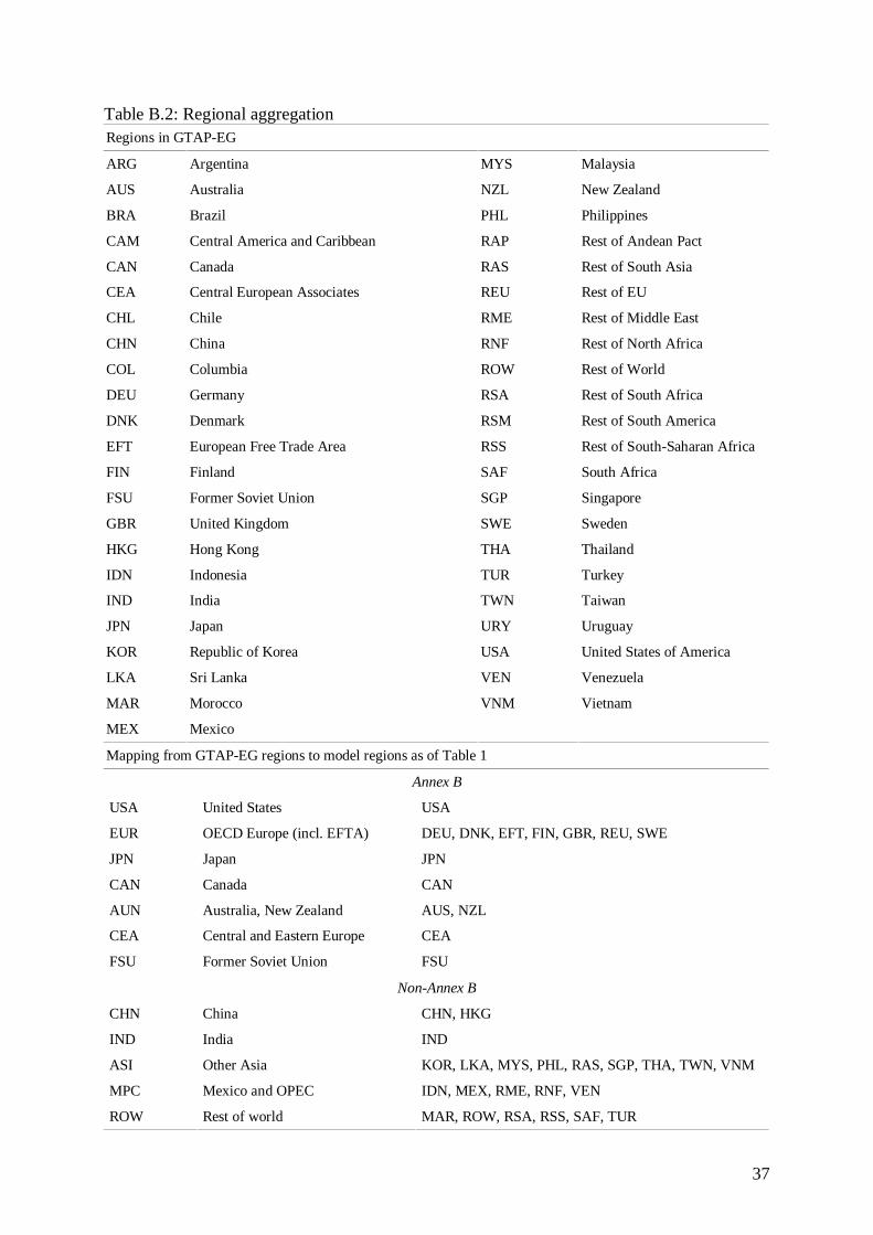
Table B.2: Regional aggregationRegions in GTAP-EG

ARG Argentina MYS Malaysia

AUS Australia NZL New Zealand

BRA Brazil PHL Philippines

CAM Central America and Caribbean RAP Rest of Andean Pact

CAN Canada RAS Rest of South Asia

CEA Central European Associates REU Rest of EU

CHL Chile RME Rest of Middle East

CHN China RNF Rest of North Africa

COL Columbia ROW Rest of World

DEU Germany RSA Rest of South Africa

DNK Denmark RSM Rest of South America

EFT European Free Trade Area RSS Rest of South-Saharan Africa

FIN Finland SAF South Africa

FSU Former Soviet Union SGP Singapore

GBR United Kingdom SWE Sweden

HKG Hong Kong THA Thailand

IDN Indonesia TUR Turkey

IND India TWN Taiwan

JPN Japan URY Uruguay

KOR Republic of Korea USA United States of America

LKA Sri Lanka VEN Venezuela

MAR Morocco VNM Vietnam

MEX Mexico

Mapping from GTAP-EG regions to model regions as of Table 1

Annex B

USA United States USA

EUR OECD Europe (incl. EFTA) DEU, DNK, EFT, FIN, GBR, REU, SWE

JPN Japan JPN

CAN Canada CAN

AUN Australia, New Zealand AUS, NZL

CEA Central and Eastern Europe CEA

FSU Former Soviet Union FSU

Non-Annex B

CHN China CHN, HKG

IND India IND

ASI Other Asia KOR, LKA, MYS, PHL, RAS, SGP, THA, TWN, VNM

MPC Mexico and OPEC IDN, MEX, RME, RNF, VEN

ROW Rest of world MAR, ROW, RSA, RSS, SAF, TUR

38

Appendix C: GHG Emission Reduction Targets for Annex B countries

Labela Original Kyoto Targets (OLD)b


Revised Targets (NEW)c


Australia AUN 108 110.7

Austria EUR 87 92.9

Belgium EUR 92.5 93.8

Bulgaria CEA 92 95.2

Canada CAN 94 107.9

Croatia CEA 95 95

Czech Republic CEA 92 94.1

Denmark EUR 79 81.1

Estonia FSU 92 94.7

Finland EUR 100 107.8

France EUR 100 103.9

Germany EUR 79 80.7

Greece EUR 125 133.1

Hungary CEA 94 97.8

Iceland EUR 110 118

Ireland EUR 113 116.2

Italy EUR 93.5 95.3

Japan JPN 94 99.2

Latvia FSU 92 98

Liechtenstein EUR 92 107.9

Lithuania EUR 92 96.5

Luxemburg EUR 72 79.6

Monaco EUR 92 93

Netherlands EUR 94 95.2

New Zealand AUN 100 107

Norway EUR 101 105.3

Poland CEA 94 96.5

Portugal EUR 127 130.7

Romania CEA 92 96.2

Russian Federation FSU 100 105.7

Slovakia CEA 92 96.3

Slovenia CEA 92 100.4

Spain EUR 115 118.9

Sweden EUR 104 109.5

Switzerland EUR 92 96.6

Ukraine FSU 100 102.4

United Kingdom EUR 87.5 88.8

United States USA 93 96.8a Label of aggregate model region which includes the respective Annex B countryb UNFCCC (1997)c Estimates by the European Commission accounting for sink credits as agreed in Bonn and Marrakesh (Nemry 2001)

climate politics from kyoto to bonn: from little to...

Documents