climate change in australia | regional report › media... · australian climate change projections...

BANANA PLANTATION AFTER CYCLONE YASI, QUEENSLAND, ISTOCK

CHAPTER NINE

USING CLIMATE CHANGE DATA IN IMPACT ASSESSMENT AND ADAPTATION PLANNING

9 CHAPTER 9 USING CLIMATE CHANGE DATA IN IMPACT ASSESSMENT AND ADAPTATION PLANNING

Climate change data provide an essential input to the impact assessment process. Methods for generating, presenting and selecting data are described in this chapter, along with information to help users find data and research tools. This includes a decision tree to guide users to the most relevant material; report-ready images and tables; climate change data (such as a 10 percent decrease in rainfall relative to 1986-2005); and application-ready data (where projected changes have been applied to observed data for use in detailed impact assessments). Links are provided to other projects that supply climate change information.

9.1 INTRODUCTION

In Chapters 6, 7 and 8, climate projections derived from CMIP5 modelling experiments were evaluated and presented. Chapter 9 describes how to apply these projections in impact assessments that will inform regional NRM planning in Australia. This builds on information contained in Chapter 6 of the 2007 Climate Change in Australia technical report (CSIRO and BOM, 2007).

It is useful to distinguish between two broad types of projection information; scientific knowledge about the range of plausible climate change and datasets for use in applications. Chapters 7 and 8 of this Report include qualitative statements as well as some quantitative ranges of change, with confidence levels, about projected climate change which is represented by the path on the left of Figure 9.1. The path on the right of the figure, datasets for applications, is the focus of this chapter. The scientific knowledge product can potentially synthesise a broader range of relevant evidence than the application datasets product.

The provision of application-ready datasets is usually designed to assist users in undertaking impact assessment. It draws on similar material to the scientific knowledge product, but is restricted to modelling techniques and approaches that produce projection datasets in a form suitable for use in applications. Typically this results in only a subset of the ranges of plausible future climate change being considered. A subset may be required if users require downscaled climate data (available from limited models) or if a small number of multivariate scenarios are required (best served by single climate models).

Application-ready datasets do not always represent all changes provided by global climate models. As such, a key challenge is to ensure that application-ready data used in impact assessment are as representative as possible of current knowledge of climate change (described by the yellow arrow in Figure 9.1). Researchers should use scientific knowledge about plausible climate change (Chapters 7 and 8) in conjunction with application-ready data.

FIGURE 9.1: THE RELATIONSHIP BETWEEN THE CLIMATE PROJECTION INFORMATION PRESENTED IN CHAPTERS 7 AND 8 AND THE DATASETS FOR IMPACT ASSESSMENT APPLICATIONS DESCRIBED IN THIS CHAPTER. INFORMATION FROM GLOBAL CLIMATE MODELS (GCMS) AND DOWNSCALED OUTPUT AND OTHER SOURCES (TOP ELLIPSE) CAN BE DRAWN UPON TO INFORM OUR KNOWLEDGE OF PLAUSIBLE REGIONAL CHANGES TO CLIMATE (ELLIPSE IN THE LOWER LEFT) AND ALSO FOR USE IN IMPACT ASSESSMENTS WHERE APPLICATION OF THE INFORMATION IS REQUIRED (ELLIPSE IN THE LOWER RIGHT). THE KNOWLEDGE OF THE PLAUSIBLE REGIONAL CHANGE PROVIDES CONTEXT FOR THE DATASETS FOR APPLICATIONS, BEARING IN MIND THESE DATASETS NEED TO BE REPRESENTATIVE OF THE KNOWLEDGE.

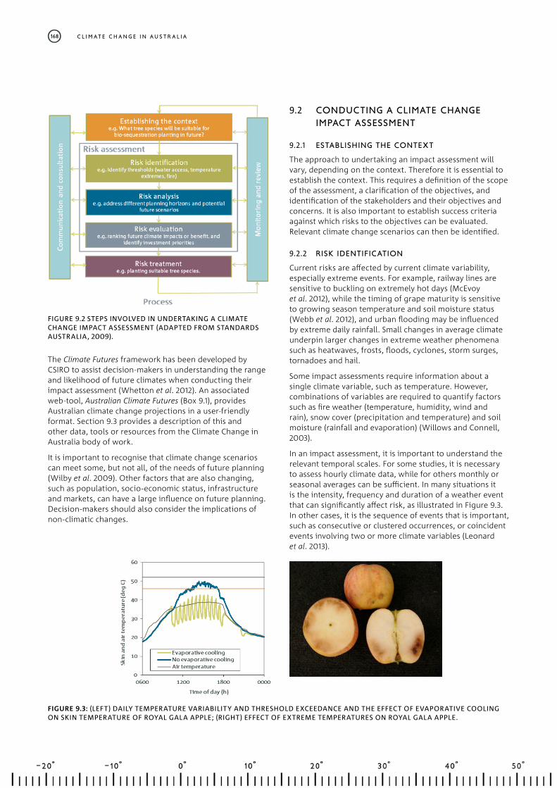
A process for undertaking a climate change impact assessment is described in Section 9.2. The series of steps in Figure 9.2 describe a robust approach to this including; establishing the context (scope and audience), identifying the known risks (within the current climate) and risk analysis (current practices and newly identified risks). These first three steps require climate information as an input. The evaluation of risks phase ranks severity and identifies areas for further analysis (not addressed in this Chapter). During risk treatment decisions are made, and emphasis should be placed on continuous monitoring of their effectiveness and reviewing lessons from the process. Other frameworks exist, but have many similarities to this simple process.

C H a p t e r N I N E 167

The Climate Futures framework has been developed by CSIRO to assist decision-makers in understanding the range and likelihood of future climates when conducting their impact assessment (Whetton et al. 2012). An associated web-tool, Australian Climate Futures (Box 9.1), provides Australian climate change projections in a user-friendly format. Section 9.3 provides a description of this and other data, tools or resources from the Climate Change in Australia body of work.

It is important to recognise that climate change scenarios can meet some, but not all, of the needs of future planning (Wilby et al. 2009). Other factors that are also changing, such as population, socio-economic status, infrastructure and markets, can have a large influence on future planning. Decision-makers should also consider the implications of non-climatic changes.

9.2 CONDUCTING A CLIMATE CHANGE IMPACT ASSESSMENT

9.2.1 ESTABLISHING THE CONTEXT

The approach to undertaking an impact assessment will vary, depending on the context. Therefore it is essential to establish the context. This requires a definition of the scope of the assessment, a clarification of the objectives, and identification of the stakeholders and their objectives and concerns. It is also important to establish success criteria against which risks to the objectives can be evaluated. Relevant climate change scenarios can then be identified.

9.2.2 RISK IDENTIFICATION

Current risks are affected by current climate variability, especially extreme events. For example, railway lines are sensitive to buckling on extremely hot days (McEvoy et al. 2012), while the timing of grape maturity is sensitive to growing season temperature and soil moisture status (Webb et al. 2012), and urban flooding may be influenced by extreme daily rainfall. Small changes in average climate underpin larger changes in extreme weather phenomena such as heatwaves, frosts, floods, cyclones, storm surges, tornadoes and hail.

Some impact assessments require information about a single climate variable, such as temperature. However, combinations of variables are required to quantify factors such as fire weather (temperature, humidity, wind and rain), snow cover (precipitation and temperature) and soil moisture (rainfall and evaporation) (Willows and Connell, 2003).

In an impact assessment, it is important to understand the relevant temporal scales. For some studies, it is necessary to assess hourly climate data, while for others monthly or seasonal averages can be sufficient. In many situations it is the intensity, frequency and duration of a weather event that can significantly affect risk, as illustrated in Figure 9.3. In other cases, it is the sequence of events that is important, such as consecutive or clustered occurrences, or coincident events involving two or more climate variables (Leonard et al. 2013).

FIGURE 9.3: (LEFT) DAILY TEMPERATURE VARIABILITY AND THRESHOLD EXCEEDANCE AND THE EFFECT OF EVAPORATIVE COOLING ON SKIN TEMPERATURE OF ROYAL GALA APPLE; (RIGHT) EFFECT OF EXTREME TEMPERATURES ON ROYAL GALA APPLE.

FIGURE 9.2 STEPS INVOLVED IN UNDERTAKING A CLIMATE CHANGE IMPACT ASSESSMENT (ADAPTED FROM STANDARDS AUSTRALIA, 2009).

C L I M AT E C H A N G E I N A U S T R A L I A168

The spatial scale required in an impact assessment will vary depending on the proposed project outcome. For example, a study on pome fruit used data from a single location in the relevant horticultural regions to describe reductions in accumulated annual chilling (exposure to cold temperatures required to break dormancy) in future climates (Darbyshire et al. 2013), whereas catchment scale information is often required in hydrological studies (CSIRO, 2008). Local government area (LGA) climate data can also be useful to align with other inputs such as population data (e.g. Baynes et al. 2013). Sometimes, even broader-scale data are sufficient for national assessments.

9.2.3 RISK ANALYSIS

The risk analysis stage includes a review of current management regimes and an analysis of the new levels of risk for different climate scenarios (Australian Greenhouse Office, 2006, Dunlop et al. 2013).

PLANNING HORIZONS

As mentioned above, changes in intensity, frequency, duration and timing are relevant across a range of temporal and spatial scales. Decisions made today will have consequences for many decades in future with regard to regional planning, land use, infrastructure investments, etc. The planning horizon will vary for different sectors. For example, when planning forest plantings for bio-sequestration of carbon emissions, the trees will be exposed to the climate in 2030 and beyond, so it is important to consider climate change projections (Figure 9.4).

CLIMATE CHANGE DATA SOURCES

Climate change projection data are usually based on output from climate models driven by various scenarios of greenhouse gas emissions, aerosols and land-use change (see Chapters 3, 7 and 8). Data can be accessed via a range of providers, such as national weather services, government departments, non-governmental organisations, academic institutions or research organisations. Identifying an appropriate dataset for use in impact assessment requires a good understanding of the pros and cons of different methods and data products (Wilby et al. 2009, Ekström et al. accepted).

The CMIP5 climate model simulations described in this Report have been undertaken using four concentration pathways, called RCP8.5, RCP6.0, RCP4.5 and RCP2.6 (Moss et al. 2010, van Vuuren et al. 2011) (see Section 3.2). Data from 16 to 39 CMIP5 models (Table 3.3.2) have been assessed and they produce a range of different projections2. Users of climate projections are strongly advised to represent a range of climate model results in their studies and reports, rather than simply using the multi-model median change or results from a single model. CSIRO’s Climate Futures approach has been developed to simplify communication and use of climate projections and to help capture the range of projection results relevant to a specified region (Whetton et al. 2012). This enables a large amount of climate model output (for a particular time period and emissions scenario) to be summarised by grouping it into a small number of categories, each of which is defined by a range of change in two climate variables such as temperature and rainfall. It is supported by the Australian Climate Futures web-tool (Box 9.1).

FIGURE 9.4: TYPICAL PLANNING HORIZONS (YEARS) FROM DIFFERENT SECTORS (SOURCE: JONES AND MCINNES, 2004).

2 NB: When conducting an impact assessment where more than one climate variable is relevant, it is inappropriate to mix projections from different models, e.g. a temperature projection from model A and a rainfall projection from model B. Only values obtained from a single model have internal consistency and are considered physically plausible.


Australian Climate Futures is a free web-based tool that provides regional climate projections for Australia (Clarke et al. 2011b, Whetton et al. 2012). It includes projections from the global climate modelling experiments that informed the IPCC’s Fourth Assessment Report (CMIP3) (IPCC, 2007) and Fifth Assessment Report (CMIP5) (IPCC, 2013) as well as a range of dynamically and statistically downscaled projections. These can be explored for up to 13 future time periods (2030, 2035, 2040..., 2085, 2090) and seven emissions scenarios (SRES: B1, A1B and A2; RCP: 2.6, 4.5, 6.0 and 8.5).

Users can explore projections for different averaging periods (e.g. monthly, seasonal, annual) and a range of climate variables for their region of interest, including:

• mean temperature • maximum temperature • minimum temperature • rainfall • downward solar radiation • relative humidity • areal potential evapotranspiration • drought• extreme daily rainfall (1 in 20 yr event)• wind-speed

Projected changes from all available climate models are classified into broad categories defined by two climate variables, e.g. the change in annual mean temperature and rainfall. Thus, model results can be sorted into different categories or ‘climate futures’, such as ‘warmer and wetter’ or ‘hotter and much drier’. The Australian Climate Futures web-tool produces a colour-coded matrix (Figure B9.1) which shows the spread and clustering in all the model results across different climate change categories, and allows users to explore how this changes under different RCPs and time periods.

Users can identify cases of particular relevance to their impact assessment, such as ‘best case’ and ‘worst’ case climate futures. In addition, it is often possible to identify

a ‘maximum consensus’ climate future in which most climate model results reside. For example, consider a study into the possible impacts of climate change on the incidence of mosquito-borne diseases in the sub-tropics. In this example, the worst case is likely to be the climate future with the greatest increase in rainfall and temperature. In Figure B9.1, the worst case is the ‘Much Hotter – Wetter’ climate future, which has low model consensus (only 2 out of 30 models) but it is a possible future that should be considered. The best case may be regarded as the ‘hotter – drier’ climate future. The maximum consensus is the ‘hotter – little change’ future.

A range of regional breakdowns, including three levels of detail based on Australia’s natural resource management regions, are available in the tool, allowing exploration of the climate futures at this scale. For example, the division of Australia into four large super-clusters allows generation of broad-scale, multi-purpose projections. In contrast, the sub-cluster boundaries allow generation of regionally relevant projections for specific purposes.

Importantly, the tool is underpinned by comprehensive climate model evaluation (Chapter 5). This ensures only those models that were found to perform satisfactorily over the Australian region are included. A few of these models were found to have limitations in particular regions only. The tool brings this information to the attention of users when relevant, and provides the opportunity to exclude those results if desired.

A key feature of Australian Climate Futures is the Representative Model Wizard. This identifies a suitable subset of models that can be used to represent the selected climate futures, e.g. a model to represent a ‘worst’ case future, one to represent a ‘best’ case future and one to represent the ‘maximum consensus’ future. For those with limited resources, this feature reduces the effort involved in analysing model data in impact studies.

BOX 9.1: AUSTRALIAN CLIMATE FUTURES


FIGURE B9.1: EXAMPLE DISPLAY OF PROJECTIONS FROM THE AUSTRALIAN CLIMATE FUTURES TOOL. THESE ARE CLASSIFIED BY ANNUAL AVERAGE CHANGES IN SURFACE TEMPERATURE AND RAINFALL, AND INCLUDE RESULTS FROM GLOBAL CLIMATE MODELS (GCMs) AND DOWNSCALING (DS). IN THIS EXAMPLE, COLOUR SHADINGS INDICATE DEGREE OF CONSENSUS AMONG THE GCM RESULTS ONLY. SOURCES OF DOWNSCALED RESULTS DISPLAYED WILL VARY WITH REGION.

METHODS FOR CREATING DATASETS FOR USE IN IMPACT ASSESSMENTS

For simple impact assessments, it may be sufficient to provide qualitative information about the direction of future climate change. For example, warmer with more extremely high temperatures, drier with more droughts, heavier daily rainfall, higher sea level, fewer but stronger cyclones, and more ocean acidification. This could facilitate a high-level scoping process, such as a workshop discussion, that identifies potential impacts and prioritises elements that may need further quantification.

Other impact assessments need quantitative information. In many cases, projected changes (relative to some reference period) are required for different years, emissions scenarios, climate variables and regions. In other cases, application-ready datasets are needed. Various methods are available for producing application-ready datasets. The choice of method must be matched to the intended application, taking into account constraints of time, resources, human capacity and supporting infrastructure (Wilby et al. 2009). A summary of some common methods for creating application-ready datasets follows, with advantages and disadvantages presented in Table 9.1.

FIGURE 9.5: FUTURE FULL BLOOM TIMING (DAY OF YEAR (DOY) OF GRANNY SMITH APPLE AFTER A WARMING OF 1, 2 OR 3 °C USING TWO DIFFERENT MODELLING METHODS, FIXED THERMAL TIME AND SEQUENTIAL CHILL GROWTH. NB. MODELLING THAT INCORPORATED CHANGES TO CHILLING ACCUMULATION (SEQUENTIAL CHILL GROWTH) INDICATED CHILL REQUIREMENTS WERE NOT FULFILLED SO NO PROJECTED FLOWERING TIMING COULD BE ESTIMATED (SOURCE: DARBYSHIRE ET AL. 2014).

PROJECTIONS DATA TYPE COVERAGE

CMIP5 GCM Australia-wide

CMIP3 GCM Australia-wide

CCAM 50km Dynamically downscaled from CMIP5 Australia-wide

BoM Analogue 5 km Statistically downscaled from CMIP5 Australia-wide

NARCliM 10 km Dynamically downscaled from CMIP3 NSW & ACT

TABLE B9.1: PROJECTIONS RESULTS REPRESENTED IN THE AUSTRALIAN CLIMATE FUTURES WEB TOOL.

The tool is fully integrated with the Climate Change in Australia website, greatly simplifying the process of displaying and downloading of datasets, GIS layers, maps and figures from the selected models.

The complete list of projections results that can be explored using the web-tool are shown in Table B9.1.

BOX 9.1 AUSTRALIAN CLIMATE FUTURES


Sensitivity analysis. This entails running a climate impact model with observed climate data to establish a baseline level of risk, then re-running the model with the same input data, modified by selected changes in climate (e.g. a warming of 1, 2 or 3 °C). This simple methodology has been effectively used to demonstrate climate change impacts in the agricultural sector (Figure 9.5) (Cullen et al. 2012, Darbyshire et al. 2014).

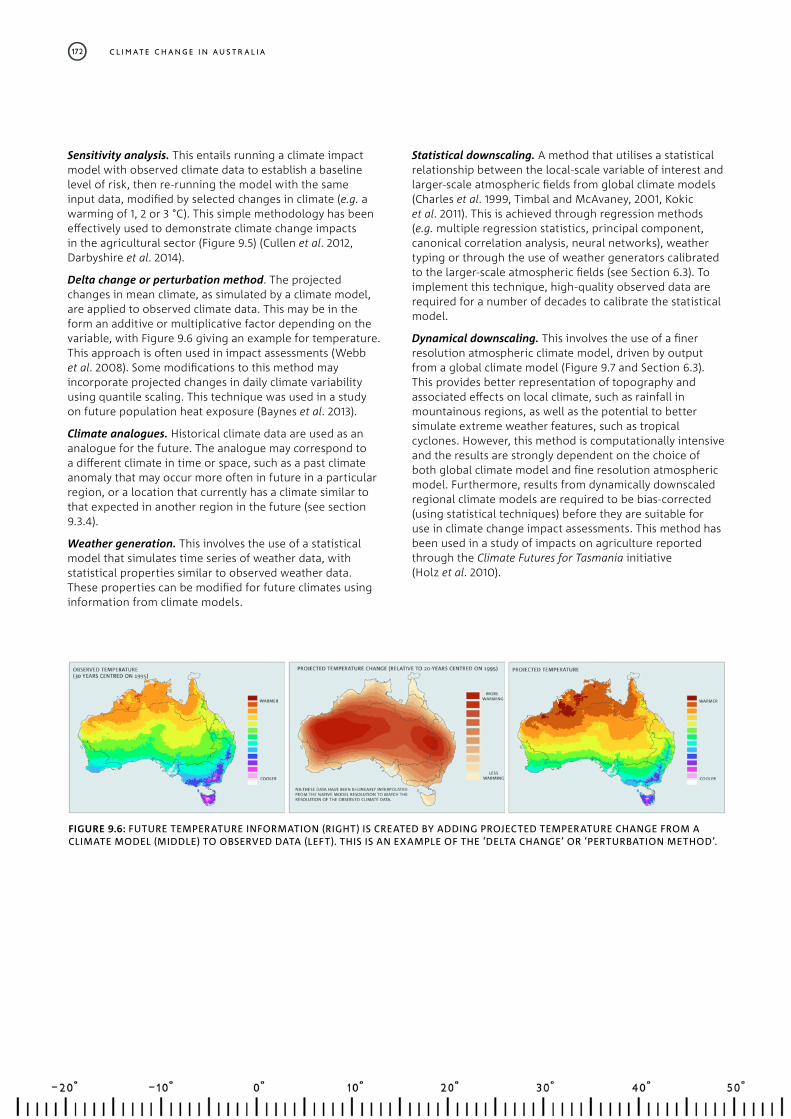
Delta change or perturbation method. The projected changes in mean climate, as simulated by a climate model, are applied to observed climate data. This may be in the form an additive or multiplicative factor depending on the variable, with Figure 9.6 giving an example for temperature. This approach is often used in impact assessments (Webb et al. 2008). Some modifications to this method may incorporate projected changes in daily climate variability using quantile scaling. This technique was used in a study on future population heat exposure (Baynes et al. 2013).

Climate analogues. Historical climate data are used as an analogue for the future. The analogue may correspond to a different climate in time or space, such as a past climate anomaly that may occur more often in future in a particular region, or a location that currently has a climate similar to that expected in another region in the future (see section 9.3.4).

Weather generation. This involves the use of a statistical model that simulates time series of weather data, with statistical properties similar to observed weather data. These properties can be modified for future climates using information from climate models.

Statistical downscaling. A method that utilises a statistical relationship between the local-scale variable of interest and larger-scale atmospheric fields from global climate models (Charles et al. 1999, Timbal and McAvaney, 2001, Kokic et al. 2011). This is achieved through regression methods (e.g. multiple regression statistics, principal component, canonical correlation analysis, neural networks), weather typing or through the use of weather generators calibrated to the larger-scale atmospheric fields (see Section 6.3). To implement this technique, high-quality observed data are required for a number of decades to calibrate the statistical model.

Dynamical downscaling. This involves the use of a finer resolution atmospheric climate model, driven by output from a global climate model (Figure 9.7 and Section 6.3). This provides better representation of topography and associated effects on local climate, such as rainfall in mountainous regions, as well as the potential to better simulate extreme weather features, such as tropical cyclones. However, this method is computationally intensive and the results are strongly dependent on the choice of both global climate model and fine resolution atmospheric model. Furthermore, results from dynamically downscaled regional climate models are required to be bias-corrected (using statistical techniques) before they are suitable for use in climate change impact assessments. This method has been used in a study of impacts on agriculture reported through the Climate Futures for Tasmania initiative (Holz et al. 2010).

FIGURE 9.6: FUTURE TEMPERATURE INFORMATION (RIGHT) IS CREATED BY ADDING PROJECTED TEMPERATURE CHANGE FROM A CLIMATE MODEL (MIDDLE) TO OBSERVED DATA (LEFT). THIS IS AN EXAMPLE OF THE ‘DELTA CHANGE’ OR ‘PERTURBATION METHOD’.


FIGURE 9.7: THE GRID SPACING AND REPRESENTATION OF TOPOGRAPHY OF TASMANIA IN A TYPICAL CMIP3 GLOBAL CLIMATE MODEL (LEFT) COMPARED TO THAT USED IN DYNAMICAL DOWNSCALING FOR THE CLIMATE FUTURES FOR TASMANIA PROJECT (HOLZ ET AL. (2010): INTERMEDIATE (MIDDLE) AND FINE (RIGHT) GRIDS FROM THE CCAM REGIONAL CLIMATE MODELS. THE COLOUR SCALE INDICATES SURFACE HEIGHT (M).

The application-ready data (described in Section 9.3.3) employed the delta change method for all variables (Section 6.3). Quantile scaling was used to create daily rainfall data that include projected changes in variance. Where appropriate, statistically and dynamically downscaled data are also accessible (see Section 9.6.1).


TABLE 9.1: SUMMARY OF TYPICAL CHARACTERISTICS ASSOCIATED WITH METHODS FOR APPLICATION OF CLIMATE PROJECTIONS. COLOUR CODING INDICATES EASE OF USE WITH BLUE BEING EASIER AND ORANGE BEING MORE DIFFICULT (SOURCE: WILBY ET AL. (2009) AND EKSTRÖM ET AL. (ACCEPTED)).

M E T H O D A DVA N TAG E S A N D D I S ADVAN TAG ES (I N I TAL I C S)

SENSITIVITY ANALYSIS Requires no future climate change information. Shows most important variables/system thresholds. Allows comparisons between studies.Impact model uncertainty seldom reported or unknown. May not be OK near complex topography and coastlines. Change in mean only. OK for some applications but not others.Represents range of change if benchmarked to other scenarios.

WEATHER GENERATORS Provide daily or sub-daily weather variables. Preserve relationships between weather variables. Already in widespread use for simulating present climate. Needs high quality observational data for calibration and verification. Assumes a constant relationship between large-scale circulation patterns and local weather. Scenarios are sensitive to choice of predictors and quality of GCM output. Scenarios are typically time-slice rather than transient. Difficulty reproducing inter-annual variability (e.g. due to ENSO) and tropical weather phenomena such as monsoons and tropical cyclones.

DELTA CHANGE METHOD Simple to implement and suitable for many applications.Facilitates assessment of outputs from a large number of GCMsLimited applicability where changes in variance are important.May not capture projected climate behaviour around complex topography.

DELTA CHANGE METHOD (INCLUDING FUTURE CHANGES TO VARIABILITY, E.G. QUANTILE SCALING)

Suitable for many applicationsIncludes changes in variability that may be important for adequately simulating extreme eventsRequires statistical expertise to implementMay not capture projected climate behaviour around complex topography.

STATISTICAL DOWNSCALING Good for many applications, but restricted by availability of relevant variables. Site-specific time-series and other statistics, e.g. extreme event frequencies. Good near high topography.Requires high quality observational data over a number of decades for calibration and verification. Assumes a constant relationship between large-scale circulation patterns and local weather. Scenarios are sensitive to choice of forcing factors and host GCM or RCM. Choice of host GCM or RCM constrained by archived outputs. Hard to choose from the large variety of methods, each with pros and cons. Need to be aware of any shortcomings of the particular method chosen.

DYNAMICAL DOWNSCALING WITH BIAS CORRECTION

Provides regional climate scenarios at 10-60 km resolution. Reflects underlying land-surface controls and feedbacks. Preserves relationships between weather variables. Often gives better representation of coastal and mountain effects, and extreme weather events. Simulations with bias-corrected SSTs should make the present-climate simulation more realistic than the host GCM. Requires high quality observational data for model verification. Should not be assumed that the dynamically downscaled projections are necessarily more reliable than projections based on the host model.High computational demand. Projections are sensitive to choice of host GCM and RCM.

DYNAMICAL DOWNSCALING CHANGE FACTOR METHOD APPLIED TO HIGH RES. OBS.

As for dynamical downscaling with bias correction. This technique is suitable for many agricultural and biodiversity applications.


9.2.4 RISK EVALUATION AND RISK TREATMENT

After risks have been analysed, it is important to rank the risks in terms of their severity. In some cases it is possible to screen out minor risks that can be set aside and identify those risks for which more detailed analysis is recommended (Australian Greenhouse Office, 2006). This should include social and economic analysis. Risk treatment is the identification of relevant options to manage the risks and their consequences, selecting the best options for incorporating into forward plans, and implementing them (Australian Greenhouse Office, 2006).

9.3 INFORMATION PRODUCTS FOR RISK IDENTIFICATION AND ANALYSIS

9.3.1 CLIMATE CHANGE IN AUSTRALIA WEBSITE

The Climate Change in Australia website, produced in parallel with this Report, provides users with extensive access to information on climate change science, climate projections, data sources and regional impacts and adaptation resources.

The website includes broad narratives about Australia’s future climate, information resources (such as downloadable reports, videos and images), guidance on using climate change projections for research, tips for users who are involved in communicating about climate change within regional communities, tools to support planning and climate decision making, and data mining interfaces to enhance the discoverability of national and regional climate change projections.

Several web interfaces allow users to search for additional climate change projection information that is not described in this Report. This is particularly relevant to users who want to explore alternative time slices, require more information about changes to a variable of interest, or require access to the underpinning climate data. Data exploration interfaces include the ability to look at selected climate thresholds, regional climate analogues, data tables, map-based information, as well as the opportunity to download climate change data (relative to a ‘present’ baseline) and application-ready data for impact studies.

As described in Chapter 2, the regionalisation scheme used to develop narratives and deliver data has been tailored to Australia’s natural resource management (NRM) sector. The website also utilises this scheme and provides access to regional climate change impacts and adaptation information through linking with relevant Australian research projects. These projects are focused on providing resources to assist in the development of natural resource management plans.

9.3.2 DECISION TREE

A decision tree underlies the architecture of the Climate Change in Australia website, and allows users to find the type of climate change information appropriate to their impact assessment (Figure 9.8). Through this mechanism users are led to sources of data, reports, background information and guidance material that may be useful in undertaking an impact assessment. This type of tool has been used successfully in the UK (Street et al. 2009, Steynor et al. 2012).


FIGURE 9.8: DECISION TREE AVAILABLE ON THE CLIMATECHANGEINAUSTRALIA.GOV.AU WEBSITE, WITHIN WHICH THE MAP EXPLORER PROVIDES A PATHWAY TO THE DOWNLOADABLE DATA PROVIDED FOR THE NRM PROJECT. PALE GREY BOX INDICATES REGISTRATION REQUIREMENT FOR ACCESS TO DATA AND INFORMATION.


9.3.3 REPORT-READY PROJECTED CHANGE INFORMATION

In many cases, simple figures and tables are all that might be required for insertion into a report, or for a presentation. Along with figures for model specific results for all of the variables, time periods and spatial scales, images and tables are also provided for ensembles of models, indicating ranges of projected change for regional averages. Images for model-specific results are also provided for all of the variables, time periods and spatial scales described in Tables 9.2 and 9.3, along with supporting text.

9.3.4 CLIMATE DATA

Two types of data are delivered to users:

• Projected climate changes (relative to the IPCC reference period 1986–2005);

• Application-ready future climate data (where projected climate changes are applied to 30 years’ of observed data).

Data are provided in varying levels of spatial detail to suit different purposes: Area averaged data are provided for the NRM domains (super-clusters, clusters and sub-clusters); nation-wide gridded data; and point data for selected localities. The CMIP5 models used in this assessment have an average spatial resolution (spacing between data points) of approximately 180km (ranging from 67km to 333km). The projected change data are available at the original grid resolution for each model. For application-ready data, bi-linear interpolation has been used to produce finer 5 km gridded resolution data to align with the grid resolution of the AWAP baseline climate dataset. Although these data look more detailed when re-gridded to a finer scale, the process of bi-linear interpolation does not add extra information, and therefore is not more accurate than the coarser resolution data.

PROJECTED CLIMATE CHANGE DATA

Projected climate change data are informative for impact assessment and are made available as described in Table 9.2. The changes are relative to 1986-2005, and based on CMIP5 global climate models and downscaling where appropriate. Annual, seasonal and monthly changes are supplied for 20-year periods centred on 2030, 2050, 2070 and 2090 for most variables and RCPs.

APPLICATION-READY DATA

Application-ready data are synthetic future data, generated by combining projected changes with observed data. These data can be used in detailed impact assessments when appropriate observed climate data are available (having sufficient quality and duration). Projected climate changes derived from eight CMIP5 models (see Box 9.2 and Figures 9.9 and 9.10) have been applied to 30-year observed datasets centred on 1995 (1981-2010)3 using the delta change method described in Section 9.2.3 for most variables.

The daily rainfall time series produced for the NRM project, however, uses a multi-timeframe quantile-quantile (MQQ) scaling approach. Using this technique, a change to daily rainfall variability, as well as the mean, is produced. Changes at longer timeframes are also of interest to many applications, such as year to year variability. The MQQ method allows the projected changes in variability (over different time-scales) as indicated by climate model outputs to be expressed in the dataset by calculating eleven distinct change factors between the baseline and future period. A unique change factor is calculated for each of eleven time-windows examined in a wavelet multi-resolution decomposition (Percival and Mofjeld, 1997, Li et al. 2012). These change factors are then applied to the observed dataset to scale up or down at each of these different timeframes.

Application-ready data include averages and time series over a range of spatial scales, as shown in Table 9.3, and they can be accessed through a range of ‘interfaces’ with guidance available via the decision tree (Figure 9.8).

Engagement with NRM sector professionals and researchers led to recommendations for delivery of data that would align with various ecological and plant production modelling tools. Bioclimatic model developers identified a number of data requirements that have been addressed to maximise the integration with the climate projections products. In response to this engagement, monthly climate projection data for ‘Bioclim’ variables (Sutherst et al. 2007), ANUCLIM compatibility (Xu and Hutchinson, 2011) and text file format suitable for use in impacts modelling e.g. the crop modelling package APSIM (McCown et al. 1996) were recognised as a useful addition to the outputs from this project.

3 To minimise the influence of natural variability on observed climate averages over the baseline period, for example the recent south-east Australian drought, a 30-year baseline dataset is used, i.e. an extended period centred on 1995.


TABLE 9.2: PROJECTED CHANGE DATA FOR DIFFERENT CLIMATE VARIABLES AND A VARIETY OF TEMPORAL AND SPATIAL SCALES, FOR 20-YEAR PERIODS CENTRED ON 2030, 2050, 2070 AND 2090, RELATIVE TO A 20-YEAR PERIOD CENTRED ON 1995 (1986-2005). GRIDDED CHANGES ARE AVAILABLE FOR INDIVIDUAL CLIMATE MODELS, FOR ALL FOUR RCPs WHERE POSSIBLE, ON THE ORIGINAL CLIMATE MODEL GRID. GREEN = AVAILABLE, GOLD = INFORMATION IN TECHNICAL AND CLUSTER REPORTS, WHITE = NOT AVAILABLE.

A Gridded changes will be available for individual climate models on the original climate model grid.

B Event is defined as 24-hour total rainfall.

C These data are considered an interim product and will be updated using higher resolution models and reported in the Australian rainfall and runoff (ARR) handbook (anticipated 2015).

D Standardised Precipitation Index, a probability index that considers precipitation only. Drought projections available for 20 models (RCP4.5 and RCP8.5) and 13 models for RCP2.6 (see McKee et al., 1993 for a description of the method for calculation of the SPI).

E Fire-weather data are supplied at 39 sites for three models (see Data Delivery Brochure).

F Data for 16 tide gauge sites (see Data Delivery Brochure), not for individual models but for a multi-model range defined by the 5th to 95th percentile.

G Event is defined as 24-hour total rainfall.

H No data for individual models but for a multi-model range defined by the 5th to 95th percentile.

VARIABLE ANNUAL SEASONAL MONTHLY

GRIDDED AREA AVG. GRIDDED AREA AVG. GRIDDED AREA AVG.

MEAN TEMPERATUREA

MAXIMUM DAILY TEMPERATUREA

MINIMUM DAILY TEMPERATUREA

RAINFALLA

RELATIVE HUMIDITYA

WET AREAL EVAPOTRANSPIRATIONA

SOLAR RADIATIONA

WIND-SPEEDA

EXTREME RAINFALL (INTENSITY OF 1 IN 20 YR EVENT)B,C,G

EXTREME WIND (INTENSITY OF 1 IN 20 YR EVENT)G

DROUGHT (SPI-BASEDD, DURATION, FREQUENCY, % TIME)

FIREE

SEA LEVEL RISE (MEAN AND EXTREME)F,H

SEA SURFACE TEMPERATUREH

SEA SURFACE SALINITYH

OCEAN ACIDIFICATION (ARAGONITE SATURATION)G,H

TROPICAL CYCLONE FREQUENCY/LOCATION

TROPICAL CYCLONE INTENSITY

SNOW

RUNOFF AND SOIL MOISTURE


A Thresholds presented in days per year above ‘XX’ °C (days), for example.

B Forest Fire Danger Index (FFDI) for 39 sites. Also see Data Delivery Brochure.

C For availability of data for cities and towns see Data Delivery Brochure.

D Proxy for Pan Evaporation.

Baseline datasets (1981–2010)

E Australian Water Availability Project (AWAP) time series data (0.05° grid) (Jones et al., 2009).

F CSIRO Land and Water dataset (Morton, 1983, Teng et al., 2012) (0.05° grid).

G ERA interim reanalysis (0.75° grid), but daily gridded wind data have quality control problems (Dee et al., 2011). High quality daily wind speed data used in fire weather analysis were sourced from 39 sites—see Data Delivery Brochure.

H ERA interim reanalysis (0.75° grid), but daily humidity data at cities/towns have quality control problems (Dee et al., 2011).

I ERA interim reanalysis (0.75° grid), but daily solar radiation data at cities/towns have quality control problems (Dee et al., 2011).

J Bureau of Meteorology high quality monthly pan-evaporation dataset (see Jovanovic et al. 2008).

TEMPORAL SCALE ANNUAL SEASONAL MONTHLY DAILY

SPATIAL SCALE GR

IDD

ED

CIT

Y/TO

WN

C

GR

IDD

ED

CIT

Y/TO

WN

C

GR

IDD

ED

CIT

Y/TO

WN

C

GR

IDD

ED

CIT

Y/TO

WN

C

CLIMATE VARIABLE AV

ERA

GES

TIM

E-SE

RIE

S

AV

ERA

GES

TIM

E-SE

RIE

S

AV

ERA

GES

TIM

E-SE

RIE

S

AV

ERA

GES

TIM

E-SE

RIE

S

AV

ERA

GES

TIM

E-SE

RIE

S

AV

ERA

GES

TIM

E-SE

RIE

S

TIM

E-SE

RIE

S

TIM

E-SE

RIE

S

Mean temperature (°C)E

Maximum daily temperatureE

Minimum daily temperatureE

Days above/below/between temperature thresholdsA,E

Rainfall (mm)E

Relative humidity (%)H

Point potential evapotranspirationD,J

Wet areal evapotranspiration (mm)F

Mean wind-speed (ms-1)G

Solar radiation (Wm-2)I

Fire weatherB

Fire weather days above/below/between thresholdsB

TABLE 9.3: ‘APPLICATION-READY’ FUTURE CLIMATE DATA FOR DIFFERENT CLIMATE VARIABLES AND A VARIETY OF TEMPORAL AND SPATIAL SCALES, FOR 30-YEAR PERIODS CENTRED ON 1995, 2030, 2050, 2070 AND 2090. THIS INCLUDES GRIDDED DATA AND DATA FOR CITIES AND TOWNS. DATA FOR CITIES ARE LIMITED BY AVAILABILITY OF A RELIABLE BASELINE DATASET. PROJECTIONS ARE BASED ON CHANGES FROM EIGHT CLIMATE MODELS, AND DOWNSCALING WHERE APPROPRIATE. GREEN = DATA AVAILABLE, WHITE = DATA NOT AVAILABLE.


Eight of the 40 CMIP5 models assessed in this project have been selected for use in provision of application-ready data. This facilitates efficient exploration of climate projections for Australia.

A number of steps were considered in the model selection process:

• Rejection of models that were found to have a low performance ranking across a number of metrics in Chapter 5 and in some other relevant assessments, e.g. Pacific Climate Change Science Program (Grose et al. 2014a), ENSO evaluation (Cai et al. 2014).

• Selection of models for which projection data were available for climate variables commonly used in impact assessments, for at least RCP4.5 and RCP8.5. Projections for other RCPs are included where possible.

• Amongst these, identification of models that are representative of the range of seasonal temperature and rainfall projections for a climate centred on 2050

and 2090 and RCP4.5 and RCP8.5 using the Australian Climate Futures software (see Figure B9.1 from this chapter and Whetton et al. (2012).

• Projections for wind were assessed separately from temperature and rainfall to ensure the CMIP5 range was captured. This is because the direction and magnitude of wind projections are not necessarily correlated with the temperature and/or rainfall projections.

• Availability of corresponding statistical or dynamical downscaled data.

• Consideration of the independence of the models (Knutti et al. 2013).

The eight models and the reasons for their inclusion are shown in Table B9.4. Their results are shown in context of the 40 models for temperature and rainfall over the four NRM super-clusters (see Figure 2.3) for 2050 and 2090 (Figure 9.10 and 9.11).

BOX 9.2: MODEL SELECTION FOR APPLICATION-READY DATA

SELECTED MODELS

CLIMATE FUTURES WIND OTHER

ACCESS1.0 Maximum consensus for many regions.

The model exhibited a high skill score with regard to historical climate.

CESM1-CAM5 Hotter and wetter, or hotter and least drying

This model was representative of a low change in an index of the Southern Annular Mode (per degree global warming). Further, the model has results representing all RCPs.

CNRM-CM5 Hot /wet end of range in Southern Australia

This model was representative of low warming/dry SST modes as described in Watterson (2012) (see Section 3.6). It also has a good representation of extreme El Niño in CMIP5 evaluations (see Cai et al. ( 2014)).

GFDL-ESM2M Hotter and drier model for many clusters

Greatest increase This model was representative of the hot/dry SST mode as described in (Watterson, 2012) (see Section 3.6). It also has a good representation of extreme El Niño in CMIP5 evaluations (see Cai et al. (2014)). Further, the model has results representing all RCPs.

HadGEM2-CC Maximum consensus for many regions.

Greatest reduction This model has good representation of extreme El Niño in CMIP5 evaluations (see Cai et al. (2014)

CanESM2 This model was representative of the hot/wet SST mode as described in Watterson ( 2012) (Section 3.6). It also has a high skill score with regard to historical climate and it increased representation of the spread in genealogy of models (Knutti et al., 2013). It also has good representation of extreme El Niño in CMIP5 evaluations (Cai et al., 2014).

MIROC5 (non-commercial use only)

Low warming wetter model This model was representative of a higher change in an index of the Southern Annular mode (per degree global warming). It also has good representation of extreme El Niño in CMIP5 evaluations (see Cai et al. (2014)). Further, the model has results representing all RCPs.

NorESM1-M Low warming wettest representative model

No wind data This model was representative of the low warming/wet SST mode as described in Watterson (2012) (see Section 3.6). The model also has results representing all RCPs.

TABLE B9.4: SELECTED CMIP5 MODELS AND REASONS FOR THEIR INCLUSION.


FIGURE 9.9: MID CENTURY (2050) PROJECTED TEMPERATURE CHANGE (°C, LEFT), RAINFALL RELATIVE PERCENT CHANGE (RIGHT) FOR, FROM TOP TO BOTTOM, NORTHERN AUSTRALIA, RANGELANDS, EASTERN AUSTRALIA, AND SOUTHERN AUSTRALIA SUPER-CLUSTERS. DATA FOR ANNUAL, SUMMER (DJF), AUTUMN (MAM), WINTER (JJA) AND SPRING (SON) ARE PLOTTED FROM LEFT TO RIGHT IN EACH GRAPH. BAR RANGES INDICATE 10TH TO 90TH PERCENTILE OF 20-YEAR RUNNING MEAN OF 40 CMIP5 MODELS: HISTORICAL (GREY), RCP2.6 (GREEN), RCP4.5 (BLUE) AND RCP8.5 (PURPLE). SUPERIMPOSED ON THE BARS ARE RESULTS FOR EIGHT SELECTED MODELS: ACCESS1.0 (CIRCLE), GFDL-ESM2M (TRIANGLE-UP), CNRM-CM5 (PLUS), CESM1-CAM5 (CROSS), HADGEM2-CC (DIAMOND), MIROC5 (TRIANGLE-DOWN), CANESM2 (SQUARE), AND NORESM1-M (STAR).


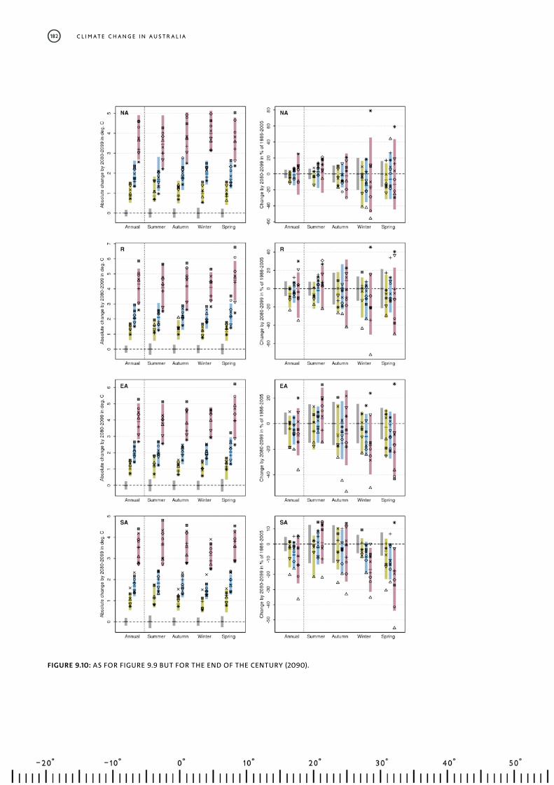
FIGURE 9.10: AS FOR FIGURE 9.9 BUT FOR THE END OF THE CENTURY (2090).


9.3.5 CLIMATE ANALOGUE TOOL

Identification of areas that experience similar climatic conditions, but which may be separated in space or time (i.e. with past or future climates) can be helpful when starting to consider adaptation strategies to a changing climate. Locating areas where the current climate is similar to the projected future climate of a place of interest (e.g. what will the future climate of Melbourne be like?) is a simple method for visualising and communicating the impact of projected changes (Hallegatte et al. 2007, Whetton et al. 2013).

The climate analogue tool available on the website is based on the approach used by Whetton et al. (2013), which matches annual average rainfall and maximum temperature (within set tolerances). This approach was also used to generate the analogue cases presented as examples in each of the Cluster Reports. These results should capture sites of broadly similar annual maximum temperature and water balance, but ignores potentially important seasonal differences in rainfall occurrences and other factors. The online tool has additional features that give the user the potential the refine the search for analogues by including measures of rainfall seasonality (per cent of annual rainfall that falls in summer) and temperature seasonality (difference in summer and winter temperature). Figure 9.11 depicts analogues after a 3 °C increase in annual maximum temperature and a 15 percent decrease in annual rainfall, e.g. where Melbourne’s future climate matches the current climate in Dubbo (NSW). Nevertheless we note that other potentially important aspects of local climate are still not matched with this approach, such as frost days or and other local climate influences, and for agriculture applications, solar radiation and soils are not considered. Thus we advise against the analogues being used directly in adaptation planning without considering more detailed information.

9.3.6 LINKS TO OTHER PROJECTS

Links to other CMIP3 based projects and sources of data are available through the website.

Information portals and State Government initiatives include:

• Climate Futures for Tasmania: This project details the general impacts of climate change in Tasmania over the 21st century, with a description of past and present climate and projections for the future. It assesses how water will flow through various Tasmanian water catchments and into storage reservoirs under different climate scenarios. It also assesses specific climate indicators most important for productivity in several key agricultural groups. Working with emergency service agencies, the project identifies the climate variables of greatest concern to emergency managers (http://www.acecrc.org.au/Research/Climate%20Futures).

• South Eastern Australian Climate Initiative: This program was established in 2005 to improve understanding of the nature and causes of climate variability and change in south-eastern Australia in order to better manage climate impacts. It concluded in September 2012 (http://www.seaci.org/).

• Indian Ocean Climate Initiative: This program investigated the causes of climate change in Western Australia and developed regional projections. It ended in 2013 (www.ioci.org.au).

• The Goyder Institute for Water Research: This program was established in 2010 to support the security and management of South Australia’s water supply and contribute to water reform in Australia. CMIP5 data are used in this project. (http://goyderinstitute.org/).

• South East Queensland Climate Adaptation Research Initiative: This program provides access to information on climate projections and adaptation options for settlements in South-east Queensland. It ended in November 2012. (http://www.griffith.edu.au/environment-planning-architecture/urban-research-program/research/south-east-queensland-climate-adaptation-research-initiative)

FIGURE 9.11: CLIMATE ANALOGUE EXAMPLE (MELBOURNE, +3 °C AND -15 % RAINFALL).


DATA PORTALS

• James Cook University Tropical Data Hub: a research data repository (https://eresearch.jcu.edu.au/tdh)

• NSW and ACT Regional Climate Modelling (NARCliM): This project is producing an ensemble of regional climate projections for south-east Australia in collaboration with the NSW Government. This ensemble is designed to provide robust projections that span the range of likely future changes in climate. A wide variety of climate variables will be available at high temporal and spatial resolution for use in impacts and adaptation research (http://www.ccrc.unsw.edu.au/NARCliM/).

• The Consistent Climate Scenarios Project: This project provides Australia-wide projections data for 2030 and 2050 as daily time-series in a format suitable for most biophysical models. It includes daily projections of rainfall, evaporation, minimum and maximum temperature, solar radiation and vapour pressure deficit for individual locations. Projections data were also developed on a 5 km grid across Australia. (http://www.longpaddock.qld.gov.au/climateprojections)

• CliMond: This is a set of free climate data products consisting of high resolution interpolated surfaces of recent historical climate and relevant future climate data. These are available at monthly time-scales, for 35 Bioclim variables, in CLIMEX format, and as the Köppen-Geiger climate classification scheme (https://www.climond.org/).

• Climate Futures for Tasmania: This project included a data portal (https://dl.tpac.org.au/tpacportal/).


climate change in australia | regional report › media... · australian climate change projections...

Documents