3.5 Climate Change Prediction

3.5 Climate Change Prediction

(i) Climate Modeling

(ii) Detection and Attribution of Climate Change

(iii) Climate Change Predictions

3

(i) Climate Modeling: The Need for Climate Models

• Test of understanding• Evaluation of response• Prediction of climate change• Attribution of causes of climate change

4

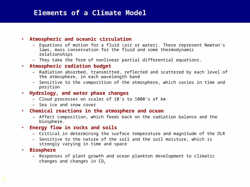
Elements of a Climate Model

• Atmospheric and oceanic circulation– Equations of motion for a fluid (air or water). These represent Newton's laws, mass

conservation for the fluid and some thermodynamic relationships– They take the form of nonlinear partial differential equations.

• Atmospheric radiation budget– Radiation absorbed, transmitted, reflected and scattered by each level of the

atmosphere, in each wavelength band– Sensitive to the composition of the atmosphere, which varies in time and position

• Hydrology, and water phase changes– Cloud processes on scales of 10's to 1000's of km– Sea ice and snow cover

• Chemical reactions in the atmosphere and ocean– Affect composition, which feeds back on the radiation balance and the biosphere.

• Energy flow in rocks and soils– Critical in determining the surface temperature and magnitude of the OLR– Sensitive to the nature of the soil and the soil moisture, which is strongly varying in

time and space

• Biosphere– Responses of plant growth and ocean plankton development to climatic changes and

changes in CO2

5

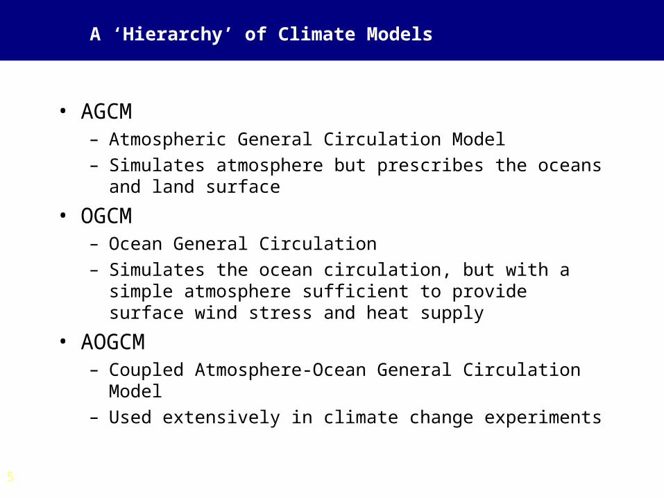
A ‘Hierarchy’ of Climate Models

• AGCM– Atmospheric General Circulation Model– Simulates atmosphere but prescribes the oceans and land

surface

• OGCM– Ocean General Circulation– Simulates the ocean circulation, but with a simple

atmosphere sufficient to provide surface wind stress and heat supply

• AOGCM– Coupled Atmosphere-Ocean General Circulation Model– Used extensively in climate change experiments

6

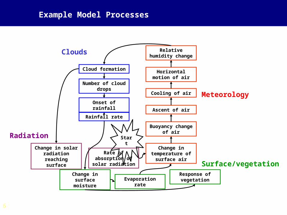
Example Model Processes

Rate of absorption of solar radiation

Change in temperature of

surface air

Buoyancy change of air

Ascent of air

Cooling of air

Horizontal motion of air

Relative humidity change

Cloud formation

Number of cloud drops

Onset of rainfall

Rainfall rate

Change in solar radiation reaching

surface

Change in surface moisture Evaporation rate

Response of vegetation

Start

Surface/vegetation

Meteorology

Clouds

Radiation

7

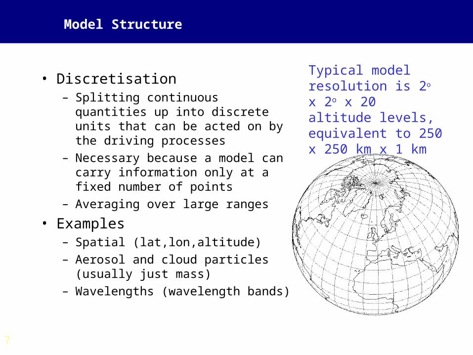
Model Structure

• Discretisation– Splitting continuous quantities up

into discrete units that can be acted on by the driving processes

– Necessary because a model can carry information only at a fixed number of points

– Averaging over large ranges

• Examples– Spatial (lat,lon,altitude)– Aerosol and cloud particles (usually

just mass)– Wavelengths (wavelength bands)

Typical model resolution is 2o x 2o x 20 altitude levels, equivalent to 250 x 250 km x 1 km

8

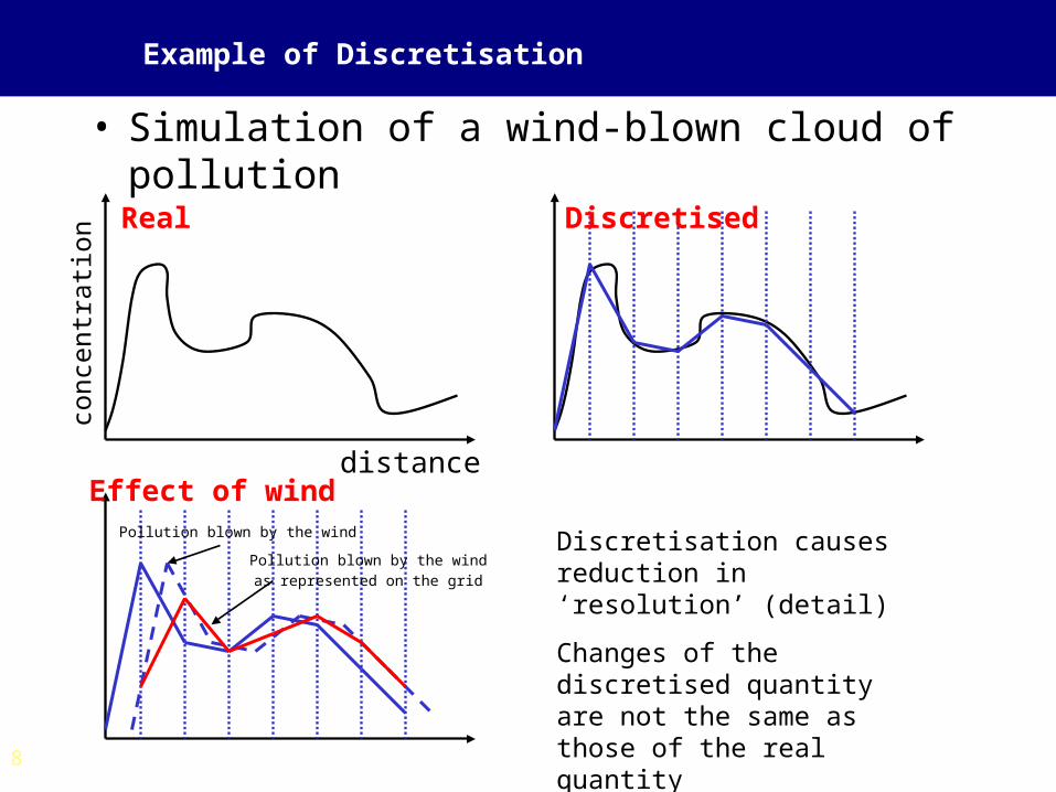
Example of Discretisation

• Simulation of a wind-blown cloud of pollution

Discretisation causes reduction in ‘resolution’ (detail)

Changes of the discretised quantity are not the same as those of the real quantity

conc

entr

atio

n

distance

Real Discretised

Effect of windPollution blown by the wind

Pollution blown by the windas represented on the grid

9

Parameterisation

• Simplification of processes in terms of simpler equations with physically or empirically derived parameters (which can be ‘tunable’)

• Example for clouds:– Rainfall assumed to occur when the liquid water content of

the cloud reaches a prescribed value – Reality is a highly complex interaction of different sized

droplets, ice crystals, hail, etc.

• Parameterisations capture the essence of real processes but they can be inaccurate and unreliable when used to make predictions under new conditions

• Almost all processes are parameterised in climate models

10

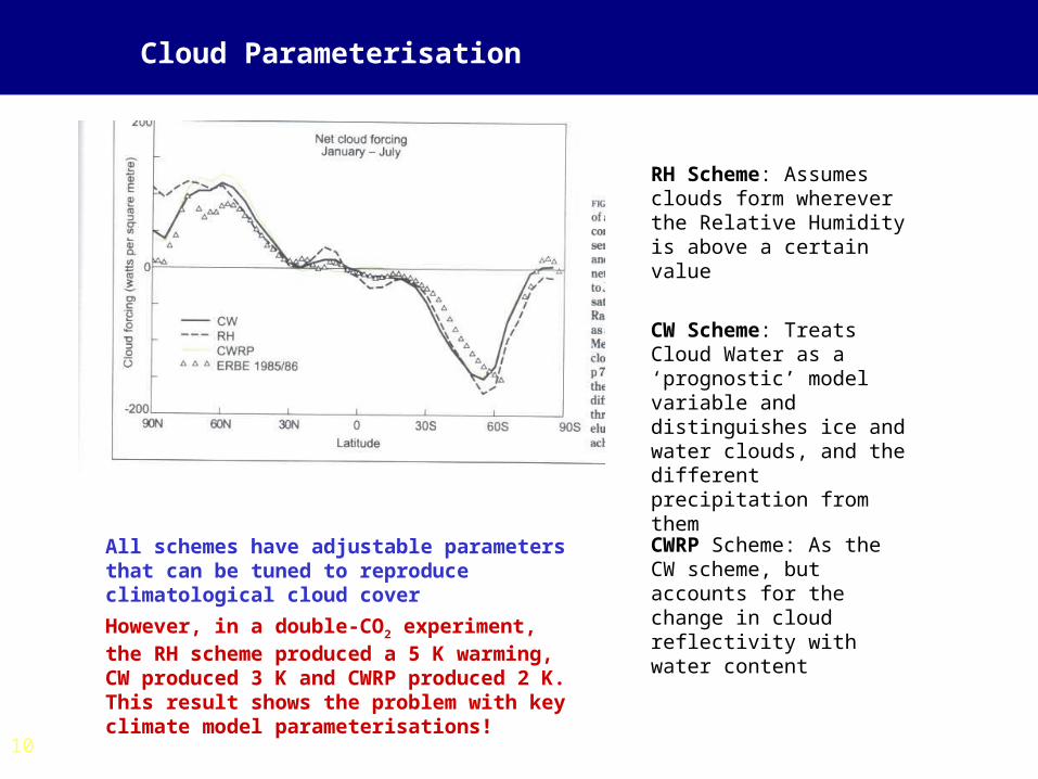
Cloud Parameterisation

RH Scheme: Assumes clouds form wherever the Relative Humidity is above a certain value

CW Scheme: Treats Cloud Water as a ‘prognostic’ model variable and distinguishes ice and water clouds, and the different precipitation from them

CWRP Scheme: As the CW scheme, but accounts for the change in cloud reflectivity with water content

All schemes have adjustable parameters that can be tuned to reproduce climatological cloud cover

However, in a double-CO2 experiment, the RH scheme produced a 5 K warming, CW produced 3 K and CWRP produced 2 K. This result shows the problem with key climate model parameterisations!

12

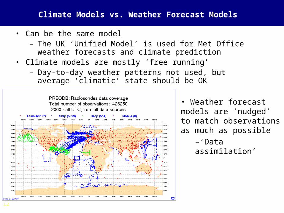
Climate Models vs. Weather Forecast Models

• Can be the same model – The UK ‘Unified Model’ is used for Met Office weather

forecasts and climate prediction• Climate models are mostly ‘free running’

– Day-to-day weather patterns not used, but average ‘climatic’ state should be OK

• Weather forecast models are ‘nudged’ to match observations as much as possible

–‘Data assimilation’

13

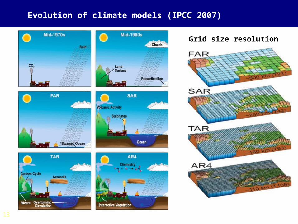
Evolution of climate models (IPCC 2007)

Grid size resolution

14

Evolution of climate models (IPCC 2007)

How has model performance improved?

IPCC (2007)

15

Two Major Problems with Early Climate Simulations

• Ocean heat ‘flux adjustments’– A non-physical ‘adjustment’ to ocean heat content to account for

incomplete ocean physics (failure to resolve narrow ocean currents, such as found in the N Atlantic)

• Cloud responses– Clouds remain one of the largest uncertainties in climate response

simulations

– Cloud feedbacks still responsible for a large part of inter-model differences – IPCC 2007

16

Model Comparisons With Observations

• Models do not simulate the current weather, but only a climatological state consistent with the prescribed forcings (greenhouse gas content of the atmosphere, aerosols, etc.)

• Need to evaluate models against average climate over, say, 1 year

• Can also look at ‘typical’ seasonal cycle or typical El Nino variations, but not for any particular year

17

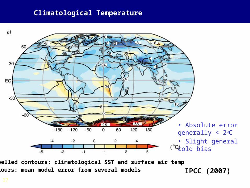
Climatological Temperature

Labelled contours: climatological SST and surface air tempColours: mean model error from several models

• Absolute error generally < 2oC• Slight general cold bias

IPCC (2007)

18

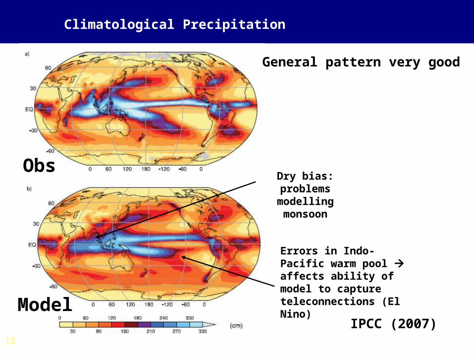
Climatological Precipitation

Obs

Model

Dry bias: problems modelling monsoon

Errors in Indo-Pacific warm pool affects ability of model to capture teleconnections (El Nino)

General pattern very good

IPCC (2007)

19

Summary of Climatological Experiments from AR4

• Confidence in model simulations has improved since previous IPCC (2001).

• Increased confidence from models no longer needing ‘flux adjustments’– These models are able to maintain stable climates

over centuries– Some biases and long-term trends remain– Tropical precipitation a problem– Clouds remain a key uncertainty in models

20

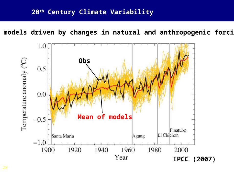
20th Century Climate Variability

58 models driven by changes in natural and anthropogenic forcings

Obs

Mean of models

IPCC (2007)

21

Simulation of ENSO

• Climate models have substantially improved spatial representation of pattern of SST anomalies in S Pacific

- Better physics

- Increased resolution• Some even used to forecast ENSO• SST gradients in equatorial Pacific still not well captured

- Thermoclines too diffuse• Most models produce ENSO variability on timescales faster than observed• Helped by further increases in model resolution?

22

Extreme Weather

• Climate models are not weather forecast models, so they can’t simulate individual events during a long simulation (of perhaps 100 years)

• We need to test the models’ variability

• Temperature: Simulation of hot and cold extremes has improved, with large regional discrepancies.

• Rainfall: Frequency of intense events and amount of precipitation during them are underestimated.

• Extra-tropical storms: These are storms affecting mid-latitude regions, such as northern Europe. These are well captured by models – improved since 2001.

• Tropical cyclones: Frequency and distribution captured well by some models – improvement since IPCC 2001

23

(ii) Detection and Attribution of Climate Change

• Anthropogenic climate change occurs against a backdrop of natural climate variability

• Internal variability– Climate variability not forced by external agents– All time-scales (weeks to centuries)

• Externally forced variability– Natural (volcanic, solar)– Anthropogenic (greenhouse gases, aerosols)– not forgetting...Changes in natural variability

• Detection of anthropogenic climate change within all this other climate variability is a statistical “signal-to-noise” problem

24

Definitions

• Detection– Demonstrating that an observed change is

significantly different (in a statistical sense) from that which can be explained by natural internal climate variability

– Detection does not imply an understanding of the causes

• Attribution– The isolation of cause and effect

25

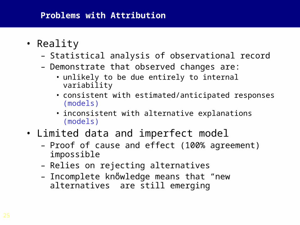
Problems with Attribution

• Reality– Statistical analysis of observational record– Demonstrate that observed changes are:

• unlikely to be due entirely to internal variability• consistent with estimated/anticipated responses (models)• inconsistent with alternative explanations (models)

• Limited data and imperfect model– Proof of cause and effect (100% agreement) impossible– Relies on rejecting alternatives– Incomplete knowledge means that “new alternatives” are still

emerging

26

Measures of Confidence Used by IPCC 2007

27

Requirements for Successful Detection and Attribution

• Good data– Sufficient coverage to identify main features of

natural variability– So far, surface and upper air temperatures have

been used– Other climate variables used for ‘qualitative’

assessment (changes broadly consistent)

28

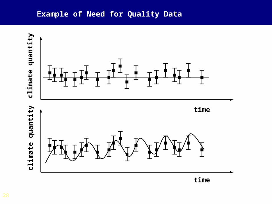
Example of Need for Quality Data

time

time

clim

ate

qu

anti

tycl

imat

e q

uan

tity

29

The Need for Long Data Records

time

clim

ate

qu

anti

ty

30

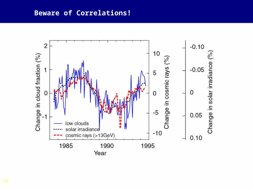
Beware of Correlations!

31

Beware of Correlations!

• Temperatures have increased since 1700 to present• The number of pirates has decreased since 1700 to present

Does this mean lack of pirates is causing climate change???

The existence of a correlation does not indicate a causal mechanism

32

Quantifying Internal Climate Variability

• From the instrumental record– Relatively short (compared to 30-50 year period of interest)– Coverage incomplete, and varies with time

• Paleoclimatic data– Reconstructions of climate before anthropogenic

perturbations– Poor resolution and global coverage– Contains unknown external forcings

• GCM ‘control’ runs over long periods (1000 years)

33

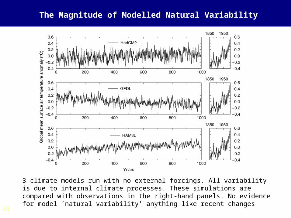
The Magnitude of Modelled Natural Variability

3 climate models run with no external forcings. All variability is due to internal climate processes. These simulations are compared with observations in the right-hand panels. No evidence for model ‘natural variability’ anything like recent changes

34

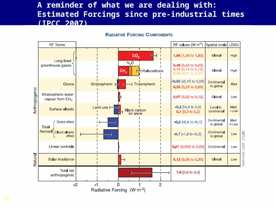
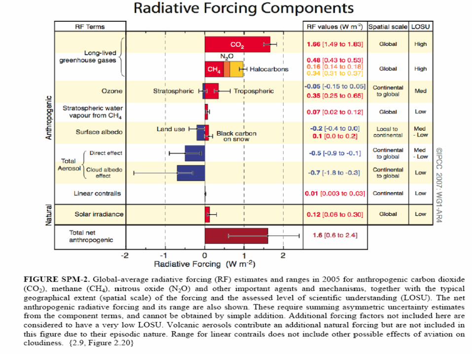
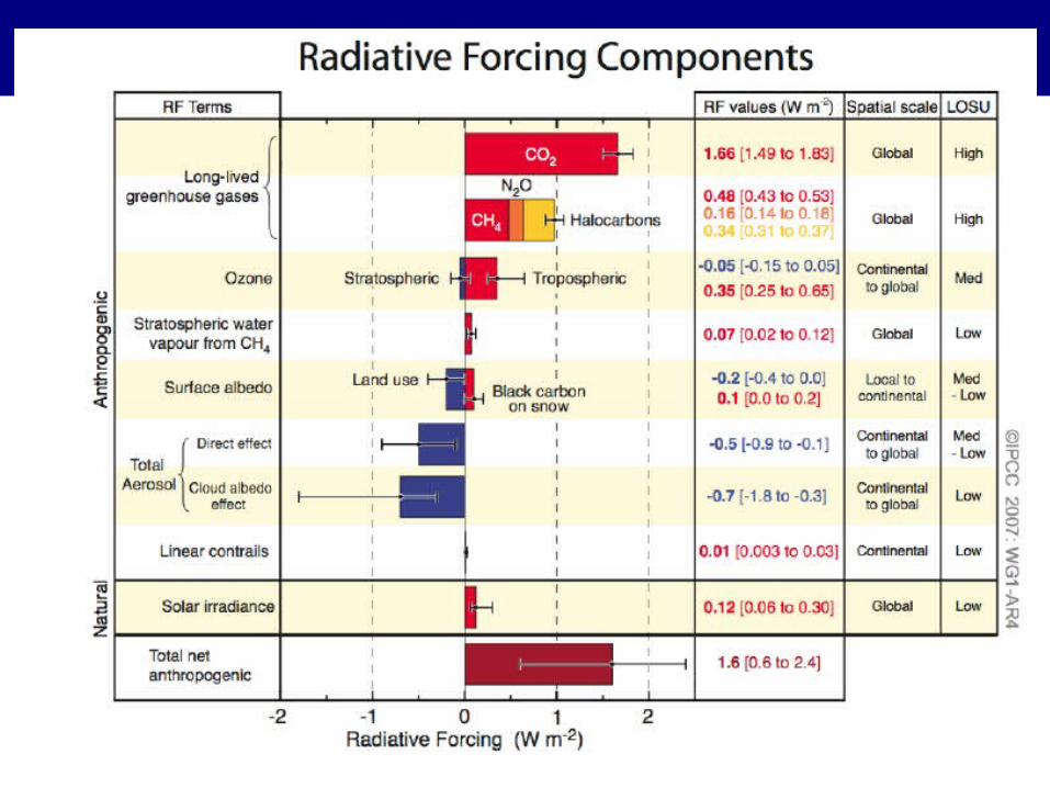
A reminder of what we are dealing with:Estimated Forcings since pre-industrial times (IPCC 2007)

Radiative Forcing

• Definition: A change in the net radiation at the top of the atmosphere due to some external factor.

Net Radiation

Net radiation = Incoming - Outgoing

Positive net radiation Incoming > Outgoing

Negative net radiation Outgoing > Incoming

Positive & Negative Forcing

• Positive forcing warming• Negative forcing cooling

Forcing and Feedbacks

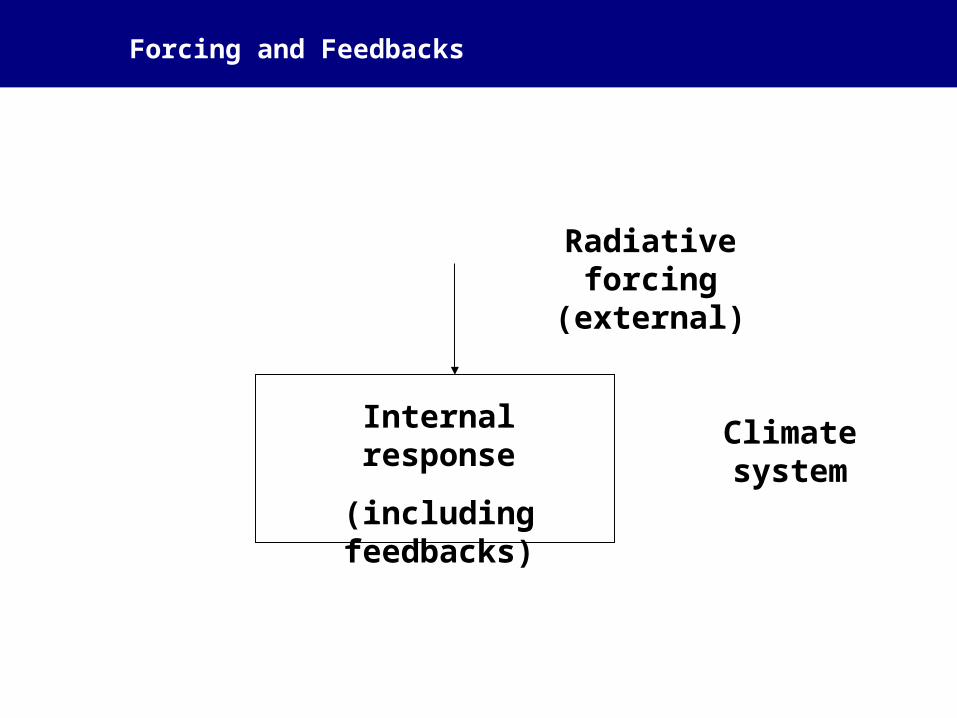
Radiative forcing (external)

Climate system

Internal response

(including feedbacks)

Forcing and Feedbacks

• “Forcing” is produced by an external process, e.g.– Changes in solar flux– Volcanic eruptions– Human actions

• A feedback is a response to temperature changes– Example: Increased water vapor due to warming

More

Anthropogenic increases in greenhouse gases are considered forcings

Increases in greenhouse gases that are caused by temperature changes are feedbacks

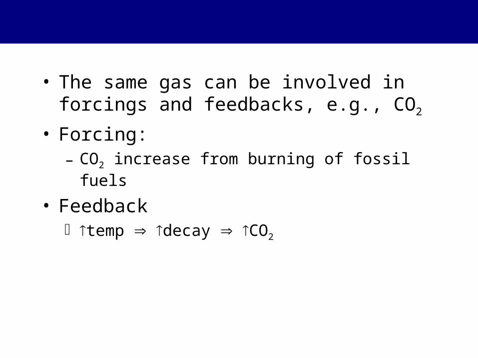
• The same gas can be involved in forcings and feedbacks, e.g., CO2

• Forcing: – CO2 increase from burning of fossil fuels

• Feedback temp decay CO2

Comparing Causes of Temperature Change

• Assumption: Larger radiative forcing larger effect on temperature

• Comparisons followSource: Intergovernmental Panel on Climate Change (IPCC)

Positive Radiative Forcings

• Largest – by far: increased greenhouse gases – Increase is almost entirely anthropogenic

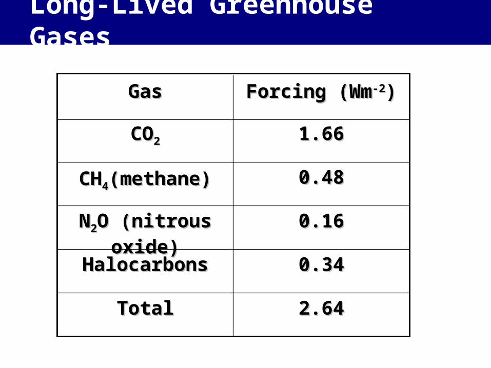
Long-Lived Greenhouse Gases

0.340.34HalocarbonsHalocarbons

2.642.64TotalTotal

0.160.16NN22O (nitrous O (nitrous

oxide)oxide)

0.480.48CHCH44(methane)(methane)

1.661.66COCO22

Forcing (WmForcing (Wm-2-2))GasGas

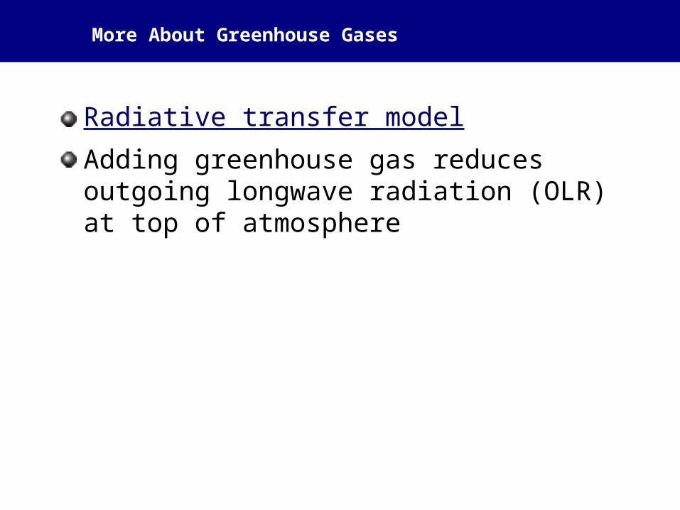
More About Greenhouse Gases

Radiative transfer model

Adding greenhouse gas reduces outgoing longwave radiation (OLR) at top of atmosphere

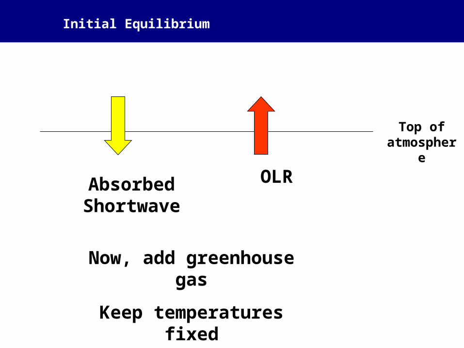
Initial Equilibrium

Absorbed Shortwave

OLR

Top of atmosphere

Now, add greenhouse gas

Keep temperatures fixed

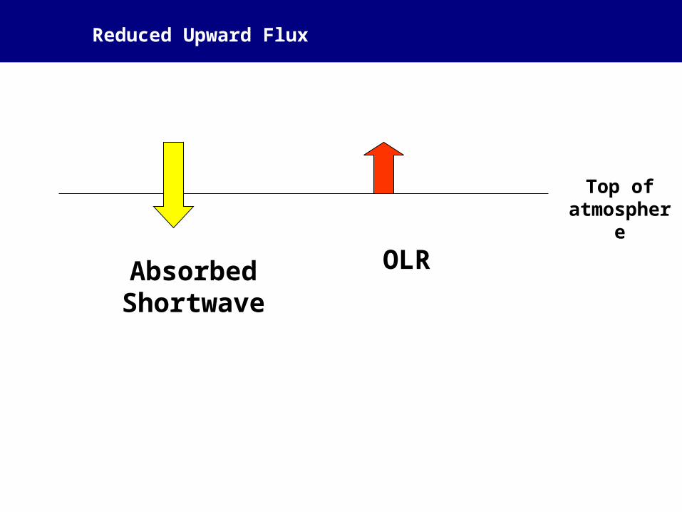
Reduced Upward Flux

Absorbed Shortwave

OLR

Top of atmosphere

Net Downward Flux

Net Flux

Top of atmosphere

Result: A positive radiative forcing

Negative Radiative Forcings

Largest: Increase in sulfate aerosols Mostly anthropogenic

Anthropogenic Sulfate Aerosols

• Coal and diesel fuel contain sulfur• Burning of these fuels produces sulfur dioxide

(a gas)• In the atmosphere, this gas is converted into

particles

Effect of Anthropogenic Sulfate Aerosols on Temperature

• Direct effect– The aerosols themselves reflect sunlight– This is similar to the effect of volcanic aerosols

• Indirect effect– Sulfate aerosols act as condensation nuclei– This increases the droplet concentration in clouds– Result: Increased cloud albedo

• Both effects tend to increase the Earth’s albedo

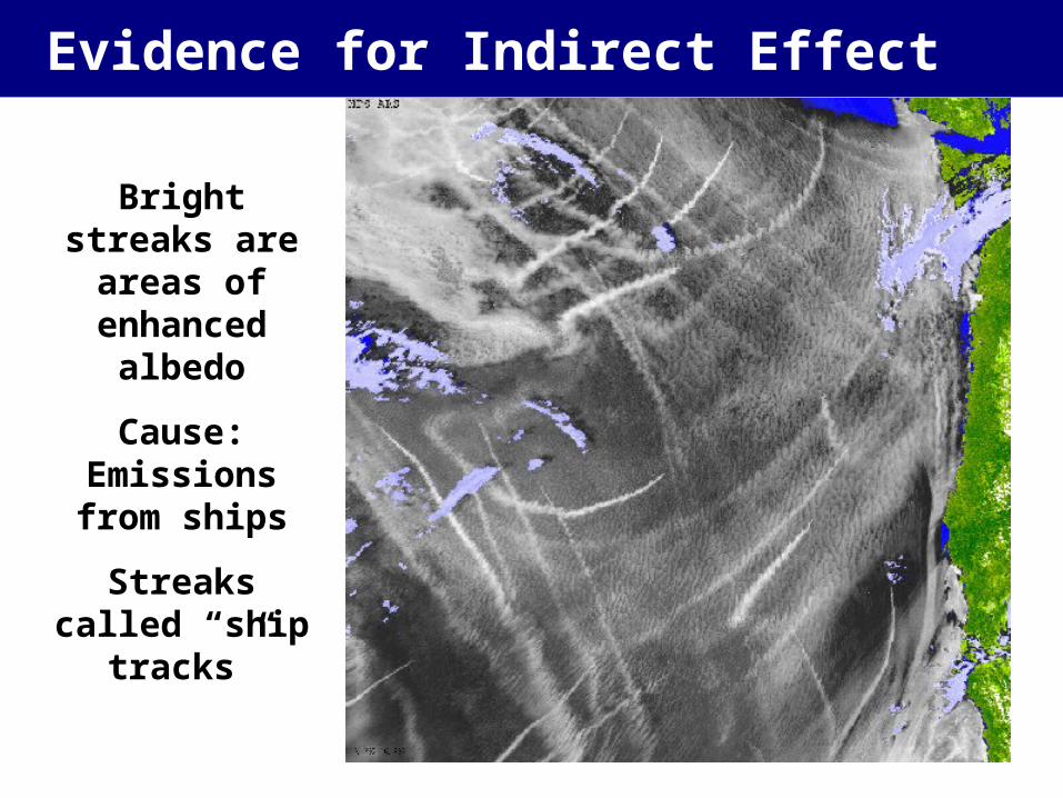
Evidence for Indirect Effect

Bright streaks are areas of

enhanced albedo

Cause: Emissions from ships

Streaks called “ship tracks”

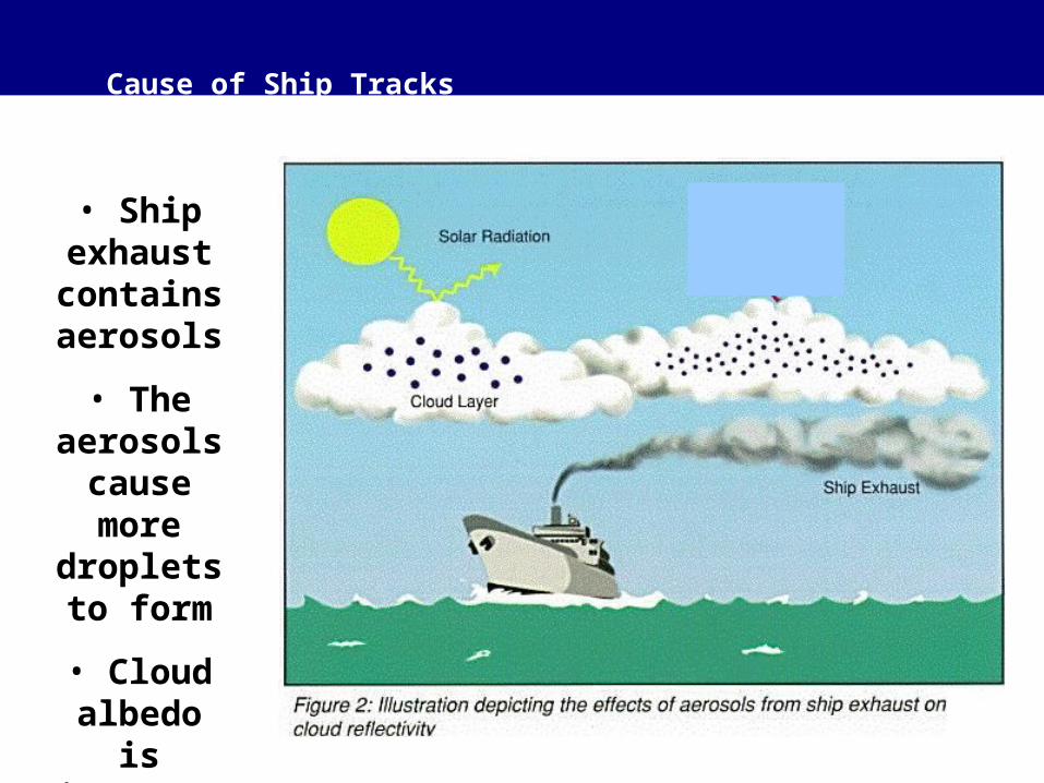
Cause of Ship Tracks

• Ship exhaust contains aerosols

• The aerosols

cause more droplets to

form

• Cloud albedo is increased

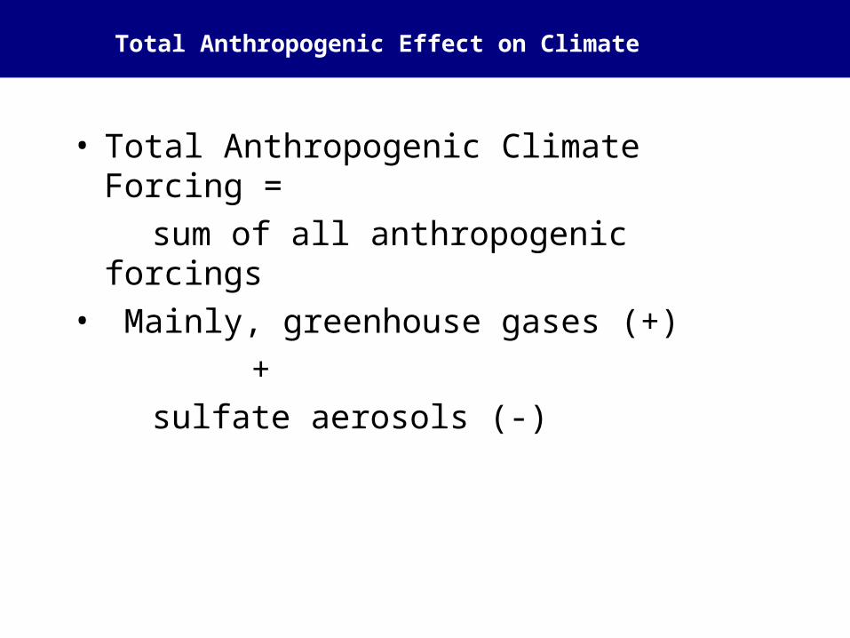
Total Anthropogenic Effect on Climate

• Total Anthropogenic Climate Forcing =

sum of all anthropogenic forcings• Mainly, greenhouse gases (+)

+

sulfate aerosols (-)

Net Anthropogenic Radiative Forcing (1750 – 2005)

Best Estimate:1.6 W/m2

Positive.

58

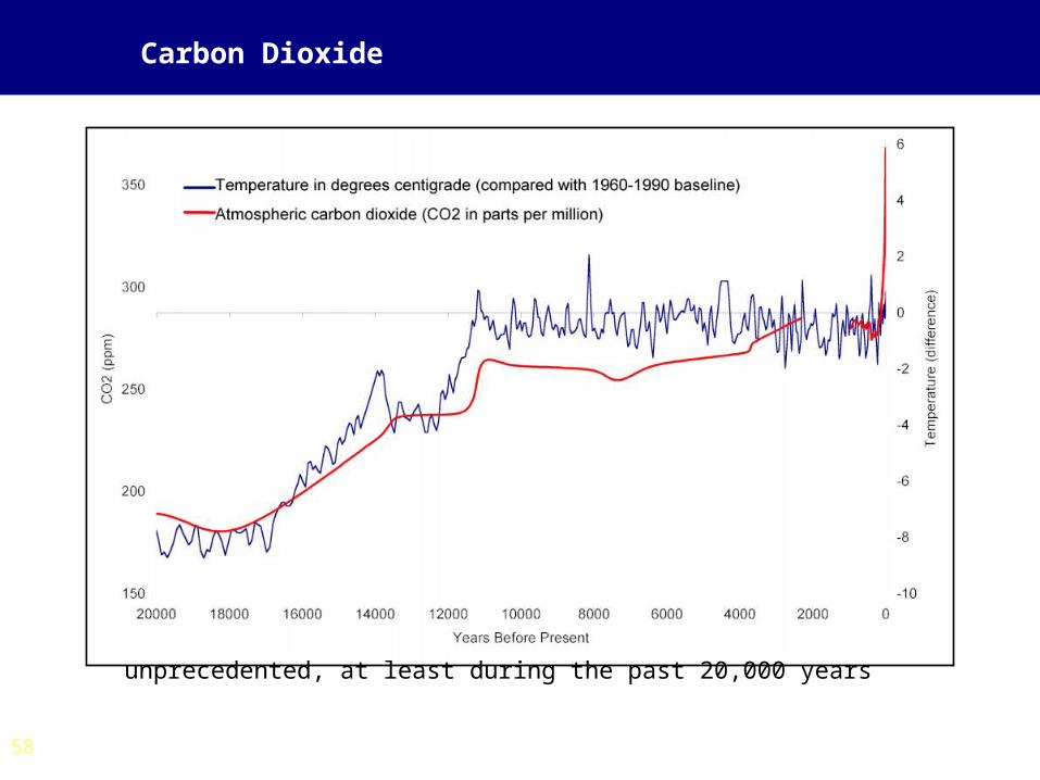
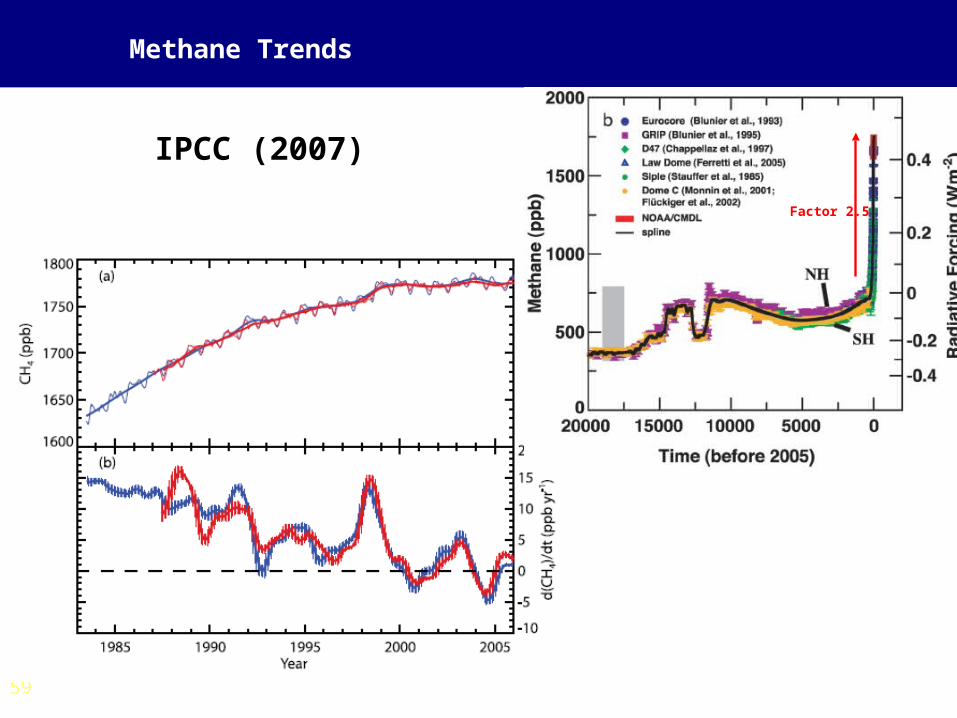
Carbon Dioxide

• From fossil fuel burning

• ~60% contribution to total radiative forcing

• Atmospheric concentration increased from 280 ppm in 1750 to 380 ppm

in 2005 (36%)

• 1999 – 2005 CO2 fossil fuel / cement emissions increased by ~3% / yr

• Today’s CO2 concentration has not been exceeded during the past

420,000 years and likely not during the past 20 million years.

• The rate of increase over the past century is unprecedented, at least

during the past 20,000 years

59

Methane Trends

IPCC (2007)

levelling off of upward trend not understood

Factor 2.5

60

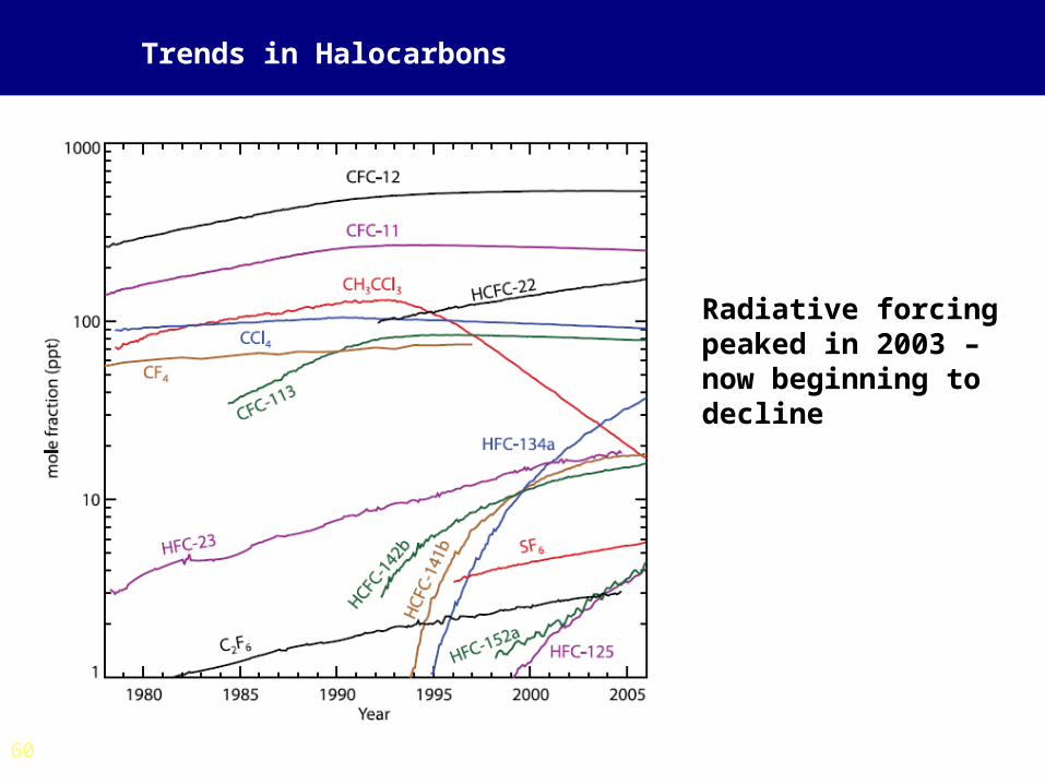
Trends in Halocarbons

Radiative forcing peaked in 2003 – now beginning to decline

61

Using Forcing-Response Relationships for Detection and Attribution

• Use the temporal and spatial variation of the different forcings

• Can separate natural and anthropogenic influences only if spatial and temporal responses are known– Climate record: Different responses are

superimposed – impossible to separate– Climate model: Study responses to individual

forcings

66

Example of model Forcing-Response Patterns

Solar Volcanic

Well mixed GHGs Ozone

Direct sulfate Total

Temp change 1890-1999 (oC / century)

67

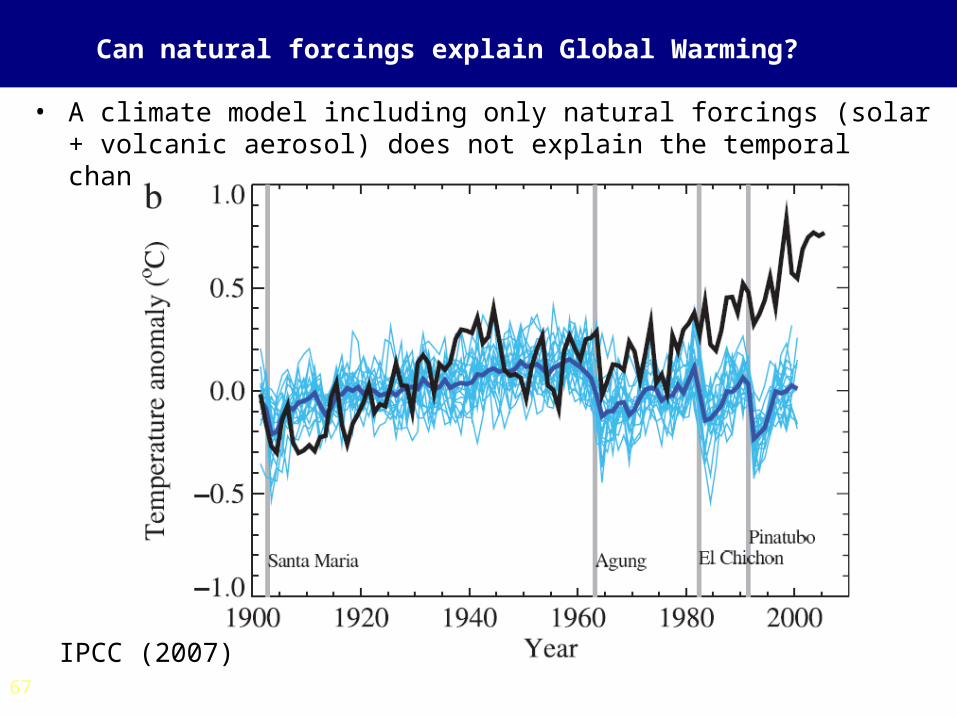
Can natural forcings explain Global Warming?

• A climate model including only natural forcings (solar + volcanic aerosol) does not explain the temporal change in global mean temperature

IPCC (2007)

68

Can natural forcings explain Global Warming?

IPCC (2007)

Models with both natural and anthropogenic forcings do far better

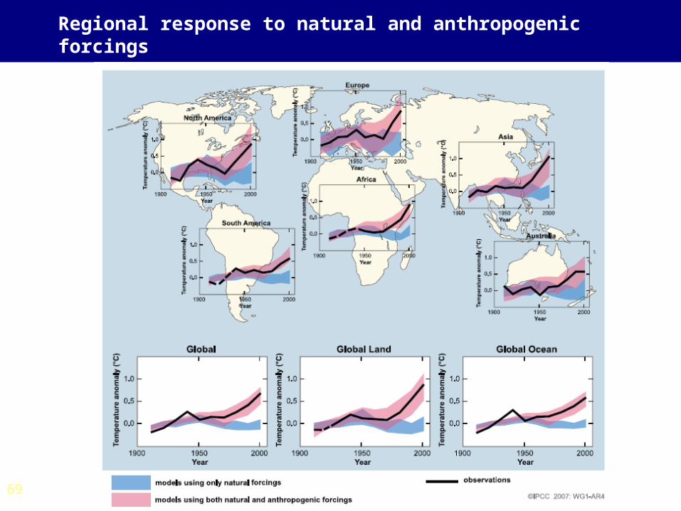
69

Regional response to natural and anthropogenic forcings

70

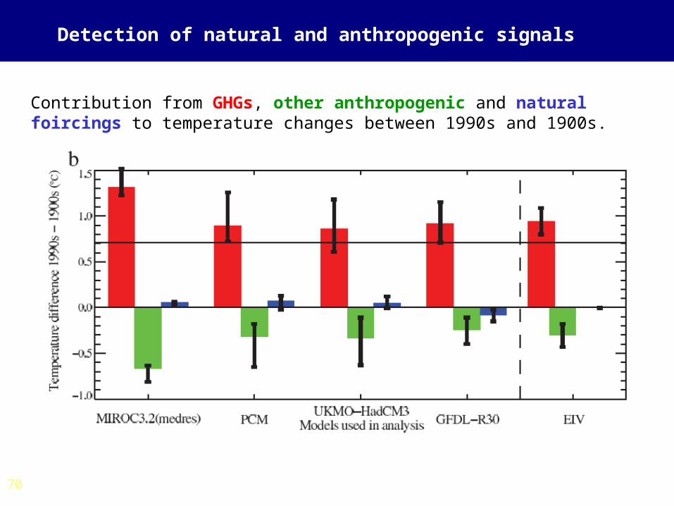
Detection of natural and anthropogenic signals

Contribution from GHGs, other anthropogenic and natural foircings to temperature changes between 1990s and 1900s.

71

Conclusions

• It is extremely unlikely (<5%) that the global pattern of warming during last 50 years can be explained without external forcing.

• Greenhouse gas forcing has very likely caused most of warming over last 50 years.

• It is likely that there has been a substantial anthropogenic contribution to surface temperature increases in every continent except Antarctica since the middle of the 20th century.

• Recommend read summary and conclusions to Chapter 9 IPCC AR4.

72

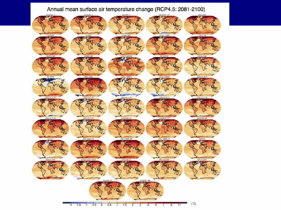
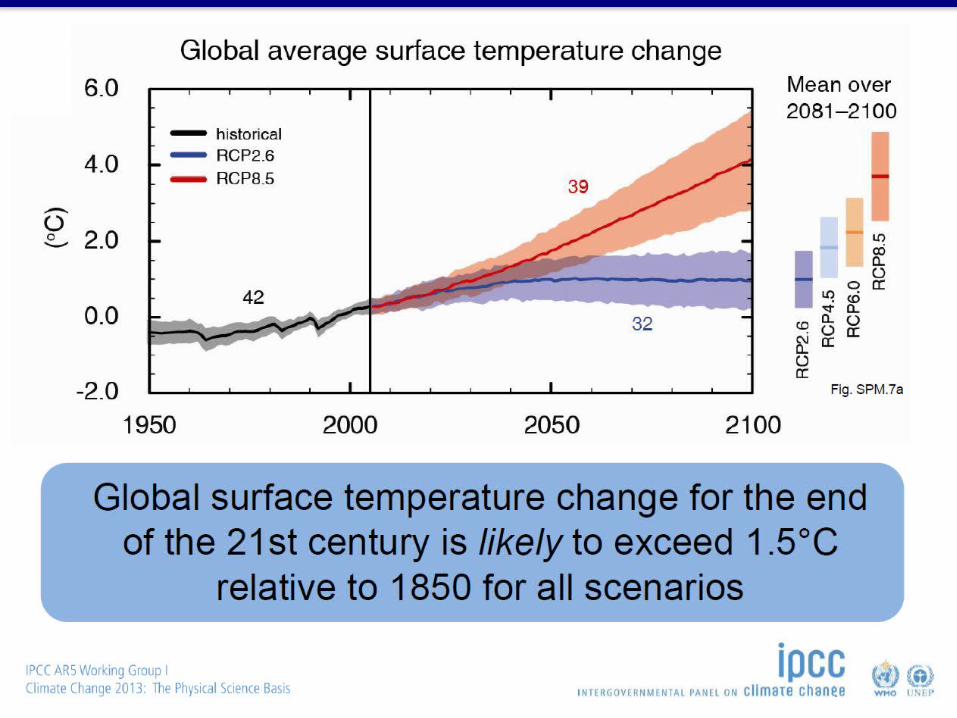
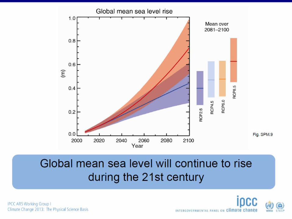
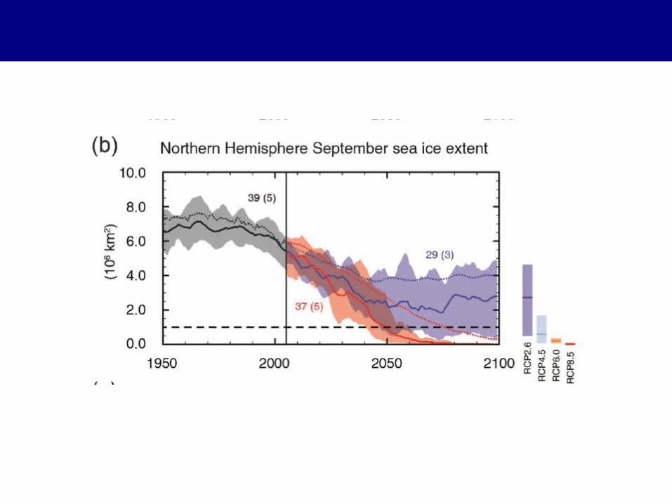
(iii) Climate Change Projections (IPCC 2013)

• Climate model experiments• Projections of future climate (IPCC AR5)

and

• ‘Geo-engineering’

IPCC AR5 - Chapter 12

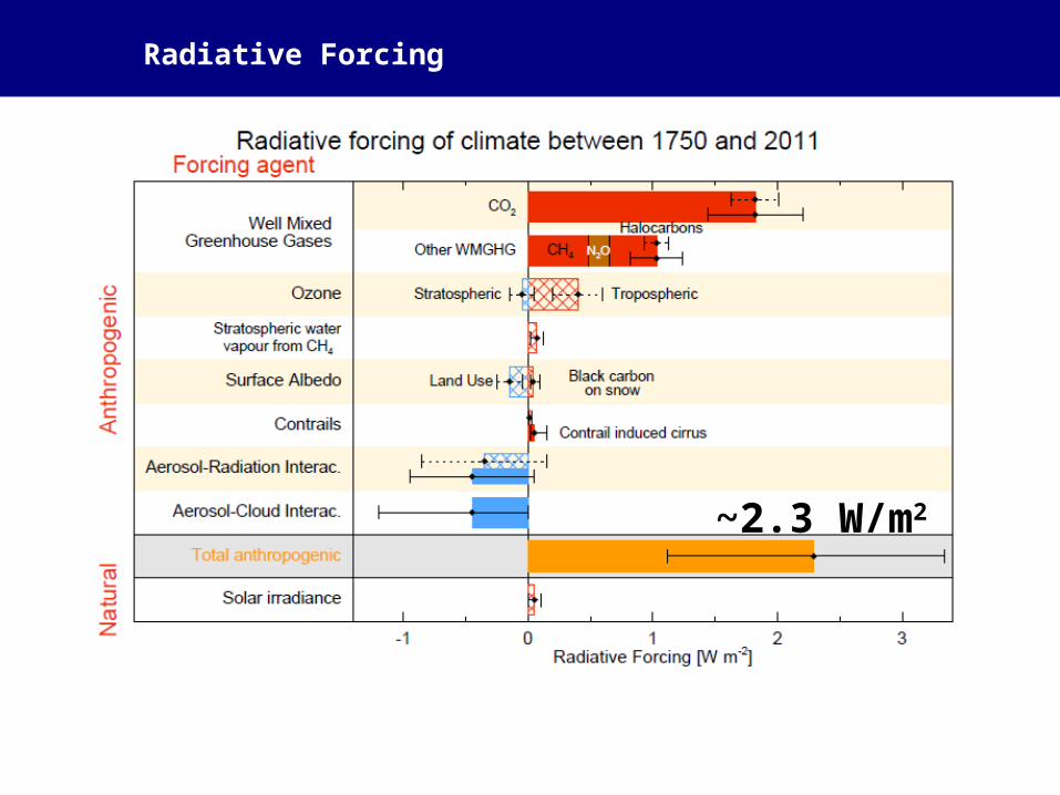
~2.3 W/m2

Radiative Forcing

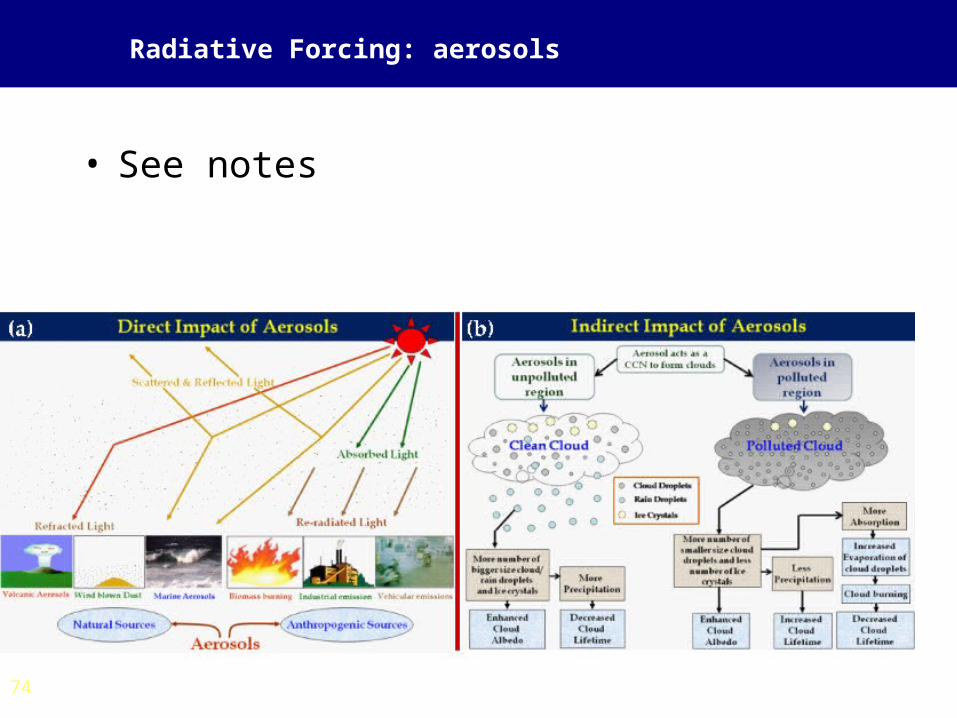
Radiative Forcing: aerosols

74

• See notes

Climate Projections

• It is not possible to make deterministic projections of future climate change.

• It is not even possible to make projections of all possible outcomes (as is “done” in medium range weather forecasting).

• Projections are uncertain because:

(i) They are primarily dependent on scenarios of future anthropogenic and natural forcings that are uncertain.

(ii) incomplete understanding and inprecise models of climate system.

(iii) Presence of internal variability.

Climate Projections

• The word “projection” is used to reflect the uncertainties and dependencies.

• Nevertheless as greenhouse gas concentations continue to rise we expect changes in the climate system to be greater than those already observed.

• It is possible to understand future climate change using models to characterise likely outcomes and uncertainties under specific assumptions about future forcing scenarios.

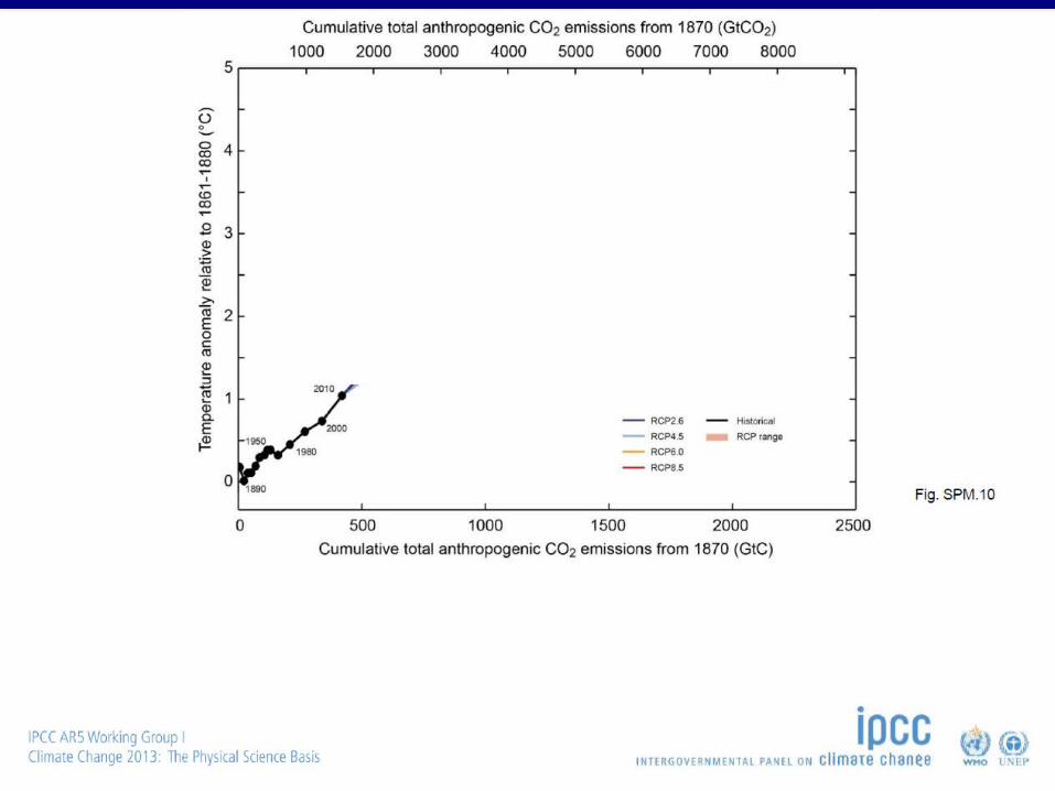
Description of Scenarios

• Previous IPCC reports based projected emissions on socio-economic scenarios – from storylines based on future demographics and economic development, regionalisation, energy production and use, technology, agriculture, forestry,and land-use. Models were then forced with an appropriate level of GHGs and aerosols.

• A new set of scenarios were created for AR5 – so-called “Representative Concentration Pathways” – these are focused on the net radiative forcing rather than on the atmospheric constituents reflecting the multiple “pathways” that can result in he same radiative forcing.

• They are defined by their net radiative forcing by 2100.

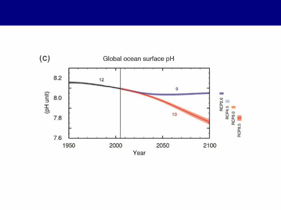
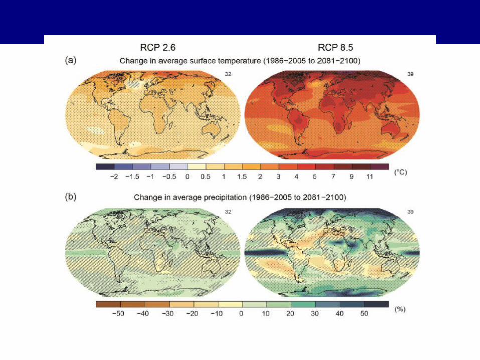
Description of Scenarios

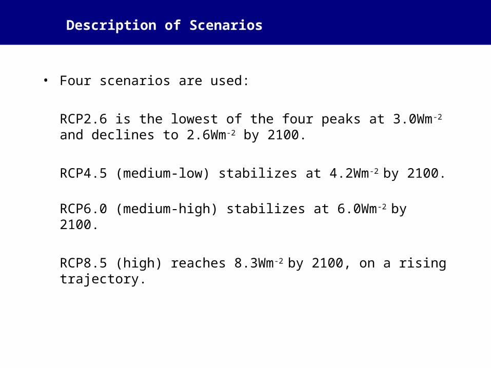
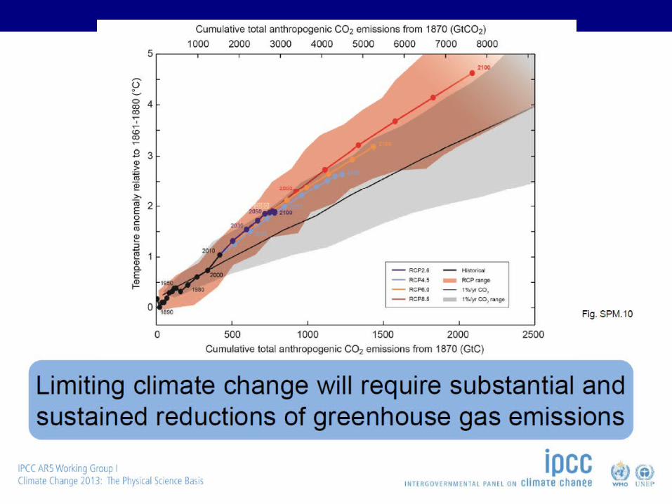
• Four scenarios are used:

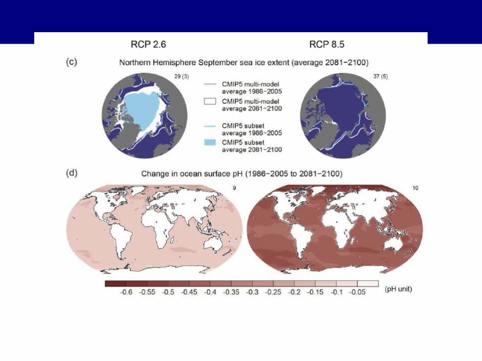
RCP2.6 is the lowest of the four peaks at 3.0Wm-2 and declines to 2.6Wm-2 by 2100.

RCP4.5 (medium-low) stabilizes at 4.2Wm-2 by 2100.

RCP6.0 (medium-high) stabilizes at 6.0Wm-2 by 2100.

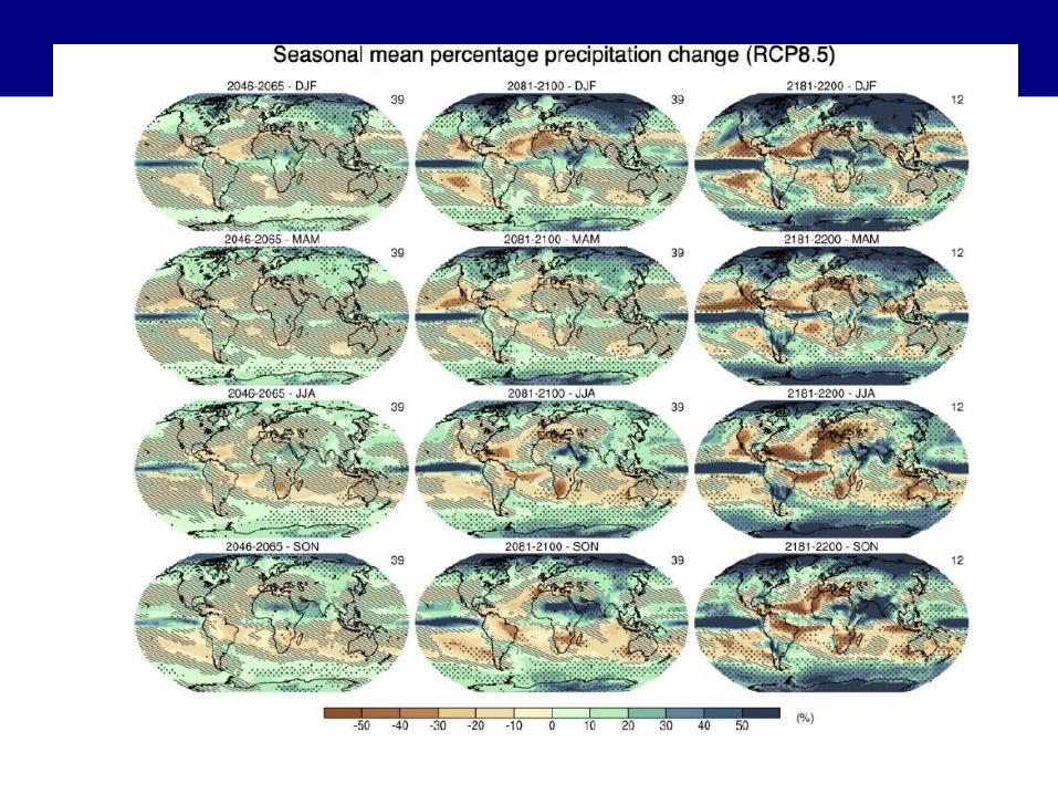
RCP8.5 (high) reaches 8.3Wm-2 by 2100, on a rising trajectory.

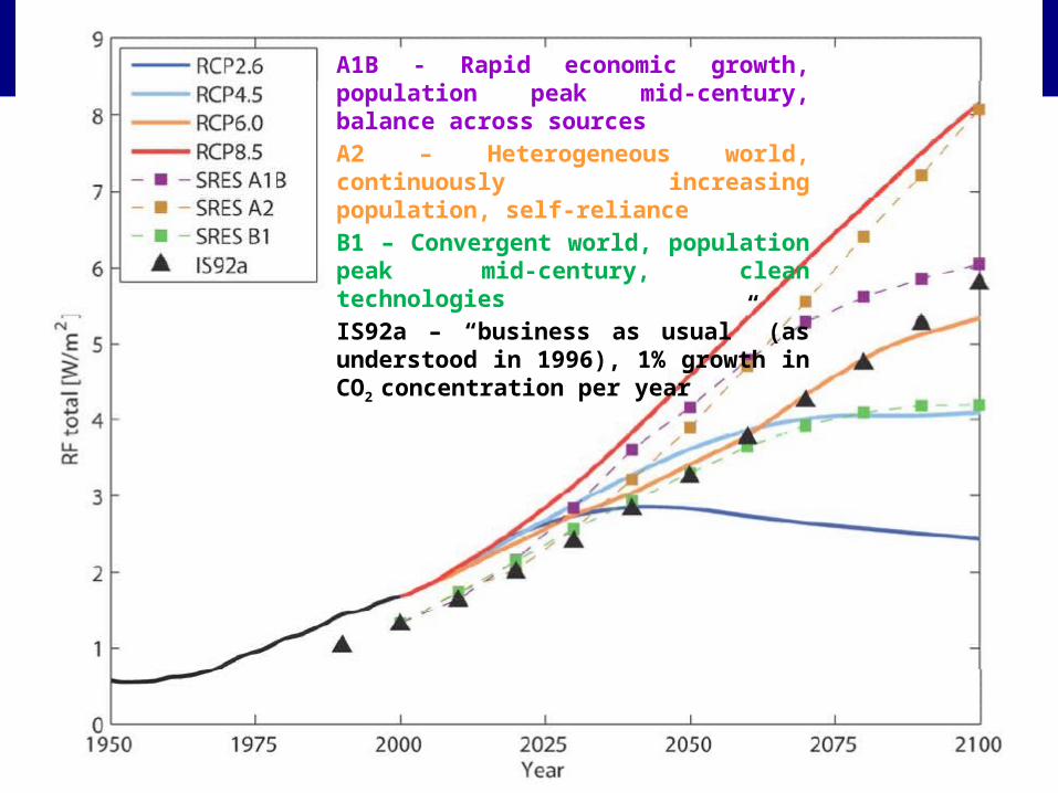
A1B - Rapid economic growth, population peak mid-century, balance across sourcesA2 – Heterogeneous world, continuously increasing population, self-relianceB1 – Convergent world, population peak mid-century, clean technologiesIS92a – “business as usual” (as understood in 1996), 1% growth in CO2

concentration per year

80

93

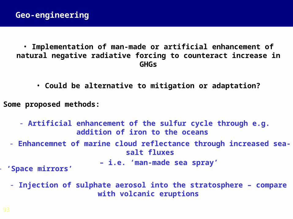
Geo-engineering

• Implementation of man-made or artificial enhancement of natural negative radiative forcing to counteract increase in GHGs

• Could be alternative to mitigation or adaptation?

Some proposed methods:

- Artificial enhancement of the sulfur cycle through e.g. addition of iron to the oceans

- Enhancemnet of marine cloud reflectance through increased sea-salt fluxes – i.e. ‘man-made sea spray’

- ‘Space mirrors’

- Injection of sulphate aerosol into the stratosphere – compare with volcanic eruptions

94

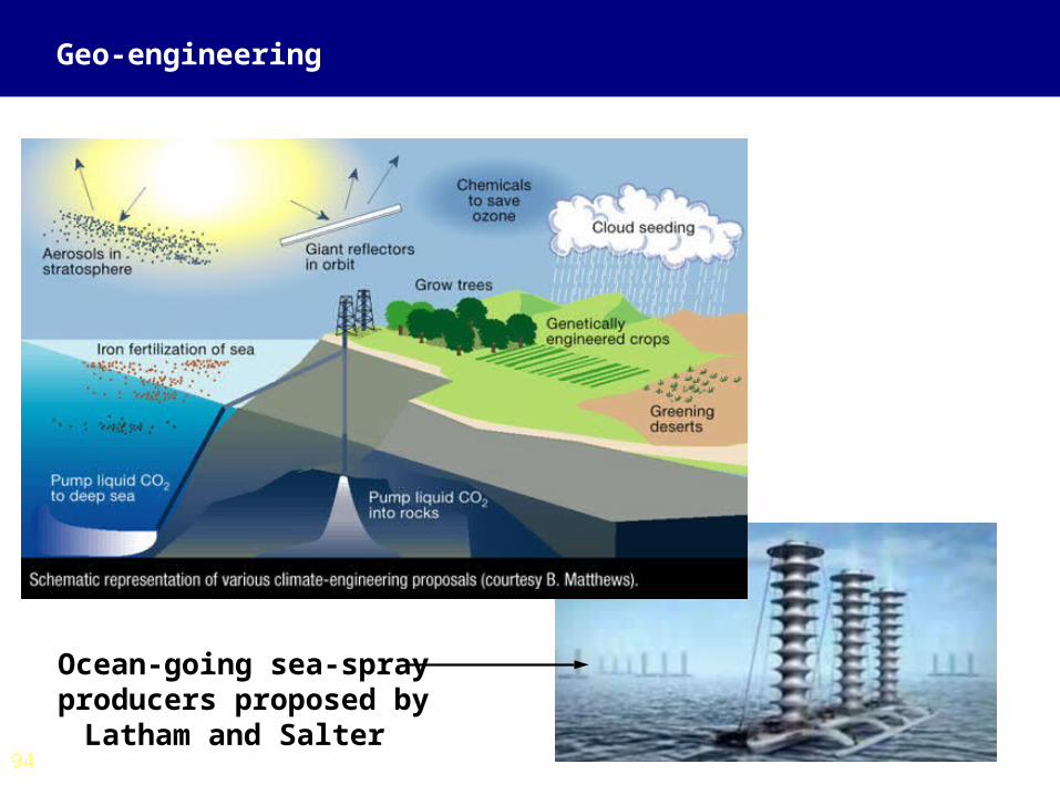
Geo-engineering

Ocean-going sea-spray producers proposed by

Latham and Salter

95

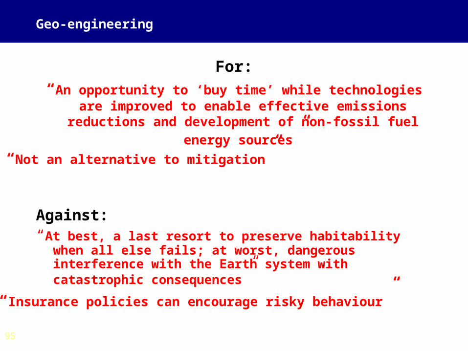
Geo-engineering

Against:“At best, a last resort to preserve habitability when all else

fails; at worst, dangerous interference with the Earth system with catastrophic consequences”

For:

“An opportunity to ‘buy time’ while technologies are improved to enable effective emissions reductions and development

of non-fossil fuel energy sources”

“Not an alternative to mitigation”

“Insurance policies can encourage risky behaviour”

96

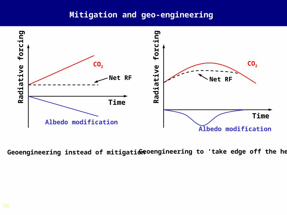
Mitigation and geo-engineering

Time

Rad

iati

ve f

orc

ing

CO2

Albedo modificationTime

Rad

iati

ve f

orc

ing

CO2

Albedo modification

Geoengineering instead of mitigation Geoengineering to ‘take edge off the heat’

Net RF Net RF

97

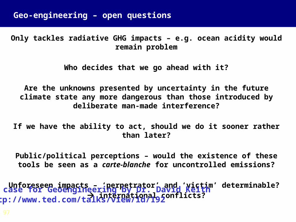
Geo-engineering – open questions

Only tackles radiative GHG impacts – e.g. ocean acidity would remain problem

Who decides that we go ahead with it?

Are the unknowns presented by uncertainty in the future climate state any more dangerous than those introduced by deliberate man-made interference?

If we have the ability to act, should we do it sooner rather than later?

Public/political perceptions – would the existence of these tools be seen as a carte-blanche for uncontrolled emissions?

Unforeseen impacts – ‘perpetrator’ and ‘victim’ determinable? international conflicts?

http://www.ted.com/talks/view/id/192The case for Geoengineering by Dr. David Keith