Chemical, Proteomic and Mechanical Characterization of

Salivary Calculi

Ana Patrícia Baptista Rodrigues

Dissertação para obtenção do Grau de Mestre em

Engenharia de Materiais

Júri

Presidente: Profª. Drª. Fernanda Maria Ramos da Cruz Margarido

Orientador: Profª. Drª. Patrícia Maria Cristovam Cipriano Almeida de Carvalho

Co-orientador: Dr. António Pedro Alves de Matos

Vogais: Prof. Dr. Arlindo Pereira de Almeida

Outubro de 2010

ii

Acknowledgements

It would not be have been possible to produce this dissertation without the help of several

people who I would like to thank.

I would like to give my thanks to my supervisor Profª. Drª. Patrícia Carvalho for all her support,

endless patience, dedication and availability. Also, to my co-supervisor Prof. Dr. Antonio Alves

de Matos, for all of his knowledge of biology, for his patience and the time spent clarifying my

doubts.

I would also like to thank my colleague Lúcia Santos for the help in all the work undertaken, her

ability and availability to discuss ideas, dedication and all the support she gave me.

I must thank Daniela Nunes and Bruno Nunes for their availability and help in conducting the

tests requiring the use of an Atomic Force Microscope.

For their help in samples preparation for use with the Transmission Electron Microscope, I

would like to thank Drª. Cristina Lacerda of the Anatomic Pathology Department, Curry Cabral

Hospital.

I would also like to thank Richard Butcher for his clarification of certain points of the English

language and for all his support.

Lastly I would like to thank my parents for all the support they have given me throughout my

academic life.

iii

Agradecimentos

Não seria possível a realização desta dissertação sem a ajuda de várias pessoas a que

gostaria de agradecer.

Gostaria de agradecer à minha orientadora Profª. Drª. Patrícia Carvalho por todo o apoio,

dedicação e disponibilidade apresentada diariamente. Ao meu co-orientador Prof. Dr. António

Alves de Matos, por todos os seus ensinamentos na área de biologia, pela sua disponibilidade

e paciência para esclarecimento de dúvidas.

Gostaria de agradecer à minha colega Lúcia Santos pela ajuda em todo o trabalho realizado,

pela sua disponibilidade, discussão de ideias, dedicação e todo o apoio que me deu.

Não podia deixar de agradecer ao Bruno Nunes e Daniela Nunes pela disponibilidade e ajuda

na realização dos ensaios no Microscópio de Força Atómica.

Pela ajuda na preparação de amostras para o Microscópio Electrónico de Transmissão gostaria

de agradecer à Drª. Cristina Lacerda do Departamento de Anatomia Patológica do Hospital

Curry Cabral.

Queria igualmente agradecer ao Richard Butcher pelos seus esclarecimentos de dúvidas sobre

a escrita inglesa e por todo o apoio.

Por último gostaria de agradecer aos meus pais por todo o apoio que me deram ao longo da

minha vida académica.

iv

Abstract

The main goal of this work is the chemical, proteomic and mechanical characterization of

sialoliths in order to explain the existence of denatured collagen, to justify the presence of

sulfur, establish a protocol for the measurement of the mechanical properties of a sialolith and

to provide new information on the calculi formation mechanism.

This study used Scanning Electron Microscopy together with X-ray maps to investigate the

morphologic and chemical aspects of a sialolith. The results showed that the sialolith was

composed of both organic matter and inorganic minerals, organized in layers around a highly

mineralized core. Transmission Electron Microscopy together with electron diffraction was also

used to screen the presence of microorganisms and to investigate crystallographic aspects of

the mineral components of the sialolith. Bacteria and globules with nanometric hydroxyapatite

crystals were found. Atomic Force Microscopy was used to probe the mechanical behaviour and

adhesivity of the sialolith components. The Electrophoresis technique was used to detect and

identify the proteins existing in sialoliths. Several proteins from leukocytes and epithelial cells,

including proteolytic enzymes, were detected. From the results obtained it has been possible to

provide new information on the role of the globular mechanism in sialolith formation.

This work contributes to a better understanding of the sialolith structure and mechanical

properties, important for the development of new techniques for the treatment of sialolithiasis.

Keywords:

Sialolith, Sialolithiasis, Scanning Electron Microscopy, Transmission Electron Microscopy,

Atomic Force Microscopy, Electrophoretic analysis.

v

Resumo

O objectivo principal deste trabalho é a caracterização química, proteómica e mecânica de

sialolitos para explicar a existência de colagénio desnaturado, para justificar a presença de

enxofre, estabelecer um protocolo para a medição das propriedades mecânicas de um sialolito

e fornecer novas informações sobre o mecanismo de formação dos sialolitos.

Para este estudo foi utilizada a Microscopia Electrónica de Varrimento em conjunto com os

mapas de raios-X, a fim de investigar os aspectos morfológicos e químicos de um sialolito. Os

resultados mostraram que o sialolito era composto por matéria orgânica e mineral, organizado

em camadas em torno do núcleo altamente mineralizado. A Microscopia Electrónica de

Transmissão em conjunto com a difracção de electrões foi usada para observar a presença de

microorganismos e investigar aspectos cristalográficos dos componentes minerais existentes

no sialolito. Bactérias e glóbulos foram encontrados contendo cristais de hidroxiapatite

nanométricos. Usando a Microscopia de Força Atómica foi possível estudar o comportamento

mecânico e adesividade dos componentes num sialolito. A técnica de Electroforese foi

utilizada para detectar e identificar as proteínas existentes no sialolito. Foram detectadas

várias proteínas de leucócitos e de células epiteliais, incluindo enzimas proteolíticas. Com os

resultados obtidos, foi possível fornecer novas informações sobre o mecanismo globular na

formação dos sialolitos.

Este trabalho contribui para uma melhor compreensão da estrutura dos sialolitos e das suas

propriedades mecânicas, importantes para o desenvolvimento de novas técnicas para o

tratamento de sialolitíase.

Palavras-chave:

Sialolito, Sialolitíase, Microscopia Electrónica de Varrimento, Microscopia Electrónica de

Transmissão, Microscopia de Força Atómica, Análise Electroforética.

vi

Contents

Acknowledgements ............................................................................... ii

Agradecimentos .................................................................................... iii

Abstract ................................................................................................. iv

Resumo ................................................................................................... v

List of Figures ..................................................................................... viii

List of tables ........................................................................................... x

List of Abbreviations ............................................................................ xi

List of Symbols .................................................................................... xii

1. Introduction ........................................................................................ 1

2. Materials and Methods ...................................................................... 6

2.1 Scanning Electron Microscopy ....................................................................... 6

2.1.1 Beam-specimen interactions - signal types ............................................ 7

2.1.2 Energy Dispersive Spectroscopy and X-ray mapping ........................... 8

2.1.3 Sample preparation .................................................................................. 9

2.2 Transmission Electron Microscopy ................................................................ 6

2.2.1 Imaging techniques ................................................................................ 10

2.2.2 Diffraction techniques ............................................................................. 11

2.2.3 Sample preparation (Ultramicrotomy) ................................................... 12

2.3 Atomic Force Microscopy .............................................................................. 15

2.3.1 Young’s Modulus and Adhesion Force ................................................. 16

2.4 Proteomic analysis ........................................................................................ 19

2.4.1 Electrophoresis ....................................................................................... 19

2.4.2 Sample Preparation ................................................................................ 20

2.4.3 Electrophoretic analysis ......................................................................... 20

2.4.4 Processing of the polypeptide bands for sequencing .......................... 20

vii

3. Results and Discussion .................................................................. 22

3.2 Scanning Electron Microscopy ..................................................................... 22

3.2 Transmission Electron Microscopy .............................................................. 29

3.3 Atomic Force Microscopy .............................................................................. 35

3.4 Proteomic analysis ........................................................................................ 40

4. Globular Mechanism ........................................................................ 42

5. Conclusion ....................................................................................... 43

6. Future work ...................................................................................... 44

7. Bibliography ..................................................................................... 45

viii

List of Figures

Figure 1 – Salivary glands [1]. ................................................................................................... 1

Figure 2 – Schematic drawing representing the globular and sedimentary cycles in the sialoliths

formation mechanism [2]. .................................................................................................. 4

Figure 3 – Schematic representation of the electron column of SEM [18]. .................................. 7

Figure 4 – Embedding procedure yielding a mounted sample, which was subsequently polished

and used for an SEM observation. The non-embedded part subjected to the

Electrophoresis technique [2]. ............................................................................................ 9

Figure 5 – Imaging techniques: Bright Field Imaging and Off-axis Dark Field [23]. ................... 11

Figure 6 – Comparison between imaging mode and diffraction mode [23]. ............................... 12

Figure 7 – Ultramicrotomy using a diamond knife [24]. ............................................................. 13

Figure 8 – Schematic of an atomic force microscope [27]. ....................................................... 15

Figure 9 - Schematic position sensitive detector current signal (IPSD) vs. piezo position (Zp) curve

including approaching and retracting parts. Three types of hysteresis can occur: In the zero

force line (A), in the contact part (B) and adhesion (C) [26]. ............................................. 17

Figure 10 - Polished cross-section of Sialolith 1a (BSE mode). ................................................ 22

Figure 11 – Detail A of Sialolith 1a polished cross-section, from where X- ray maps shown in

Figure 12 were obtained (BSE mode). ............................................................................. 23

Figure 12 – (a), (b) and (c) are the Ca, P and S X-ray maps respectively of detail A of the

Sialolith 1a polished cross-section (BSE mode). .............................................................. 24

Figure 13 – Typical EDS spectra obtained at (a) bright and (b) dark regions [2]. ...................... 24

Figure 14 – Detail B of the Sialolith 1a polished cross-section display the highly mineralized

core. The arrows indicate the teardrop globules. .............................................................. 25

Figure 15 – Detail B of the Sialolith 1a polished cross-section. Parts (a) and (b) are convolutions

of mineralized and weakly mineralized globule layers. ..................................................... 25

Figure 16 – Detail C of the Sialolith 1a polished cross-section displays the core surrounded by

an incomplete layer of organic matter with spherical globules (indicated by the arrow) (BSE

mode).............................................................................................................................. 26

Figure 17 – Detail D of the Sialolith 1a polished cross-section shows (indicated by the arrow)

the globules surrounded by crescents of smaller teardrop-shaped structures (BSE mode).

....................................................................................................................................... 26

ix

Figure 18 – Detail E of the Sialolith 1a polished cross-section. (a) Laminar layers (b) layers of

teardrop-shaped (indicated by the uppermost arrow) and spherical globules (indicated by

the lowermost arrow) (BSE mode). .................................................................................. 27

Figure 19 – Decalcified sample. (a) Organic matter without HA crystals, the arrows indicate the

spaces in organic matter where HA crystals were present before decalcification (b)

globules (Y) with a few HA crystals inside, the arrows indicate HA crystals. ..................... 29

Figure 20– Calcified sample. (a) Globules (Y) surrounded by HA crystals in organic matter and

(b) HA crystals inside a globule, the arrows indicate the HA crystals. ............................... 30

Figure 21 – Calcified sample. (a) Dark field and (b) Bright field images of HA crystals obtained in

the same region of the sample. ........................................................................................ 31

Figure 22 – The ring pattern diffraction of HA crystals obtained from a region similar to the one

presented in Figure 21. .................................................................................................... 31

Figure 23 – Calcified sample with bacteria. (a) and (b) bacteria (B). The arrow point to the

occurrence of cell division of bacteria. ............................................................................. 32

Figure 24 – Calcified sample. (a) Dark field and (b) Bright field images of HA crystals inside and

surrounding the bacteria. ................................................................................................. 33

Figure 25 – Region A of detail A of the Sialolith 1a polished cross-section obtained in BSE

mode by SEM. Region A is located in a highly mineralized area....................................... 35

Figure 26 – Region B of detail A of the Sialolith 1a polished cross-section obtained in BSE

mode by SEM. Region B is located in a weakly mineralized area. .................................... 36

Figure 27 – Topographic images of regions A (scan size: 13 μm x 13 μm) and B (scan size: 40

μm x 40 μm) from the polished cross-section. (x) and (y) are points selected in order to

obtain force-distance curves of each region. .................................................................... 36

Figure 28 – Example of the force-distance curve obtained at point x (Figure 21). Force-distance

curve describing a single approach-retract cycle of the AFM tip: (A) The AFM tip is

approaching the sample surface and the long range interactions are too small to give

measurable deflections; (B) the initial contact between the tip and the surface is mediated

by attractive Van der Waals forces (contact) that lead to an attraction of the tip toward the

surface; (C) the tip applies a constant and default force upon the surface that leads to

sample indentation, cantilever deflection and increase of repulsive forces; (D)

subsequently, the tip tries to retract and to break loose from the surface; (E) various

adhesive forces between the sample and the AFM tip, however, hamper tip retraction.

These adhesive forces can be taken directly from the force-distance curve; (F) the tip

looses contact with the surface upon overcoming of the adhesive forces [2]..................... 37

Figure 29 - Young’s (elastic) moduli of different materials. The diagram shows a spectrum from

very hard to very soft: steel > bone > collagen > protein crystals > gelatin, rubber > cells

[34]. ................................................................................................................................. 38

x

List of tables

Table 1 – Mean values (30 trials) of (N/m) and (N), and their standard deviations for the

bright and dark regions. ............................................................................................................ 37

Table 2 – Young’s modulus (MPa) for the bright and dark regions................................................ 38

Table 3 – Proteins with high molecular weight except Humam Cathepsin G (low molecular

weitht) and their accession number. ........................................................................................ 40

Table 4 – Proteins with high molecular weight and their accession number................................. 40

xi

List of Abbreviations

AFM Atomic Force Microscopy

BSE Backscattered Electrons

CPLX Calcium-Acidic Phospholipid-Phosphate Complexes

CRT Cathode Ray Tube

CT Computed Tomography

DEFA-4 Human Alpha-Defensin-4

DTT Dithiothreitol

EDS Energy Dispersive X-ray Spectroscopy

EDTA Ethylenediaminetetraacetic Acid

EISWL Endoscopic Intracorporeal Shock-Wave Lithotripsy

ESWL Extracorporeal Shock-Wave Lithotripsy

FS Force Spectroscopy

GAGs Glycosaminoglycans

HA Hydroxyapatite

HLE Human Leukocyte Elastase

HNP-4 Human Neutrophil Peptided-4

LASER or laser Light Amplification by Stimulated Emission of Radiation

LDS Lithium Dodecyl Sulphate

MALDI Matrix-Assisted Laser Desorption/Ionization

MOPS [3-(N-Morpholino) Propane Sulfonic acid]

MS Mass Spectrometry

NCBI National Center for Biotechnology Information

ND-4 Neutrophil Defensin 4

NuPAGE Novex Bis-Tris [Bis (2-hydroxyethyl) imino-tris (hydroxymethyl) methane-HCL]

SDS Sodium Dodecylsulfate

SDS-PAGE Sodium Dodecyl Sulfate Polyacrylamide Gel Electrophoresis

SE Secondary Electrons

SEM Scanning Electron Microscopy

TEM Transmission Electron Microscopy

TOF Time-Of-Flight mass spectrometer

xii

List of Symbols

contact radius (m)

interplanar spacing (m)

tip-sample distance (m)

, Young’s modulus of tip and sample material (Pa)

reduced Young’s modulus (Pa)

adhesion force (N)

spring constant cantilever (N/m)

effective spring constant (N/m)

sample Stiffness (N/m)

camera Constant

ring radius (m)

potential energy between tip and sample (J)

Hooke’s elastic potential of the cantilever (J)

tip-sample interaction potential (J)

Hooke’s elastic potential of the sample (J)

deflection of the cantilever at its end (m)

height position of the piezoelectric translator (m)

Greek letters

Indentation (m)

Wavelength (m)

Poisson’s ratio of tip and sample material (Pa)

xiii

“Godi dei tuoi successi e anche dei tuoi progetti.

Mantieni interesse per la tua professione, per quanto umile:

essa costituisce un vero patrimonio nella mutevole fortuna del tempo.”

Desiderata

1

1. Introduction

Salivary glands are the glands that secrete saliva. The three major salivary glands in the mouth

are the parotid, the submandibular and the sublingual glands, and there are two of each, one on

either side of the mouth (Figure 1). There are also other smaller salivary glands within the

cheeks and tongue. The largest salivary glands are the parotids, located below and in front of

each ear. Saliva secreted by them is discharged into the mouth through openings in the cheeks

opposite the upper teeth. The submandibular glands, located inside the lower jaw, discharge

saliva upward through openings into the floor of the mouth. The sublingual glands, beneath the

tongue, also discharge saliva into the floor of the mouth [1].

Figure 1 – Salivary glands [1].

Sialadenitis is a salivary inflammation caused by the obstruction of a salivary gland or duct, of

which one of the major causes is sialolithiasis. Sialolithiasis is the formation or presence of a

salivary calculus or sialolith in the intra or extra-glandular duct system. This disease represents

30% of all salivary pathologies, is more frequent in adults than in children, and affects 1.2% of

the general population [2].

A small sialolith that still allows saliva to flow through the duct may not cause any symptoms.

However, when a sialolith reaches a size that obstructs the passage completely, secretion by

the gland is impeded as a result of an increase in pressure, and this causes pain and swelling

2

[2, 3]. Sialoliths may also cause stasis of saliva, facilitating bacterial ascent into the gland and

subsequent infection. Long-term obstruction in the absence of infection can lead to atrophy of

the gland with resultant lack of secretory function and ultimately fibrosis [2].

Sialolithiasis is a common condition and occurs mainly in the submandibular gland (80-90% of

all cases), and to a lesser degree in the parotid gland (5-20%). The sublingual gland and the

minor salivary glands are very rarely affected [4, 5]. Single salivary calculus occur in 70-80% of

cases. Multiple sialolithiasis is rare although a few reports of it exist in the literature. Calculi can

be found in both salivary glands and ducts. Parotid calculi are found in the helium or

parenchyma of the gland in 50% of cases, while submandibular calculi are found mainly in the

duct system. The calculi vary in size and shape. Sialoliths are typically round or oval-shaped

when formed in the gland, and elongated when formed in the ducts. Parotid calculi are usually

smaller and more numerous [3]. In total, the recurrence rate of sialolithiasis has been estimated

to be 8.9% [2].

Individual differences in the structure and mineralization of sialoliths exist [2, 3]. In general,

sialoliths are composed of an organic matter and inorganic minerals distributed by a central

core and a laminar peripheral structure [3]. The nucleus of the sialolith is mostly inorganic,

predominantly made up of calcium phosphate and calcium carbonate in the form of

hydroxyapatite [Ca10(PO4)6(OH)2] although other crystallographic forms of calcium phosphate

may be present [6]. Around this amorphous nucleus laminar layers of organic and inorganic

substances (whose content varies within a single sialolith) accumulate. The organic material is

predominantly concentrated in the outer shell of a sialolith and its components are mostly

glycoproteins, mucopolysaccharides, lipids and cell detritus [2, 6]. In this region a large zone

(50-210 μm) of connective tissue and mataplastic squamous epithelium has been detected,

along with the enzymatic activity of acid phosphatase, lactate dehydrogenase, succinate

dehydrogenase and maleate dehydrogenase. Uric acid calculi may form in patients with gout.

Human submandibular-gland sialoliths contain lipids whose composition resembles that of

plasma membranes, suggesting that these lipids may originate from cell debris. Associated with

the mineral phase of submandibular sialoliths are specific lipid components, calcium-acidic

phospholipid-phosphate complexes (CPLX). These complexes induce hydroxyapatite deposition

[7]. In a recent investigation, the organic matter in the globular structures and organic strata was

found to have a high concentration of denatured collagen, probably originating from fibroblast

cell invasion and connective tissue formation in the sialolith precursor structures [2].

Salivary calculi are predominantly composed of elements including Ca, P, O, C and N, and

small amounts of Mg, Na, Cl, Si, Fe, K [2, 3]. The presence of Mg in the low concentration

facilitates precipitation of apatite crystals, which may explain the very high mineral content of

some calculi. Although a higher content of Mg inhibits crystal formation [8]. The presence of a

high sulfur content in the organic regions has been reported [2, 9] but remains unexplained.

Sulfur is an important constituent of Glycosaminoglycans (GAGs), which are present in saliva

and may be relevant in the calcification process [9].

3

The diagnosis of sialolithiasis is based on the medical history and a physical examination of the

patient. Recurrent pain and swelling of the gland, especially during meals, are common

symptoms of sialolithiasis. Imaging techniques are of fundamental importance for a positive

diagnosis: occlusal radiographs reveal radiopaque calculi, while radiolucent calculi are detected

through sialography. Ultrasound and Computed Tomography (CT) scans are other techniques

used in the detection of salivary stones [2].

Stones of the submandibular gland have a greater inorganic percentage (about 82%) than those

of the parotid gland (about 50%) and the larger the stone, the smaller the organic fraction. Many

parameters are important for the choice of therapy: the history of complications and complaints,

the position, size, and number of stones, their echogenity and adherence to the duct, and the

diameter of the duct between the stone and the papilla [2, 9]. Sialoliths can be successfully

treated by radiologically, fluoroscopically or sialendoscopically-based methods in approximately

80% of cases. Endoscopy techniques reveal a success rate of 86% in parotid sialolithotomy and

89% in submandibular sialolithotomy [2, 10]. Other non-invasive therapeutic techniques

available to treat sialolithiasis are Extracorporeal Shock-Wave Lithotripsy (ESWL) (which is

successful in up to 50% of cases) and Endoscopic Intracorporeal Shock-Wave Lithotripsy

(EISWL) (30-45%). These procedures use shock-waves to shatter salivary calculi, enabling the

fragments to pass out the duct [11] and the therapy was adopted from the lithotripsy of renal

and bladder calculi [12]. However, this method has success rates for treatment of sialolithiasis

typically lower than those achieved in the treatment of renal calculi which are essentially (95%)

calcium stones [13]. The reasons underlying this fact are still unexplained and require further

investigation. Preliminary work carried out suggests that this behaviour is related to the

ultrastructural features of salivary calculi, particularly with the presence of collagen [2, 9].

Transoral Duct Slitting is another important method used on extraparenchymal submandibular

stones, which has a success rate of 90%. Operative duct procedures and the combined

Endoscopic-Transcutaneous approach complete the spectrum of treatment possibilities for the

Parotid gland. Sialendoscopy plays a central role in the treatment of obstructive salivary gland

diseases, but maximum success can only be attained through a combination of all of these new,

minimally invasive, techniques. Through adopting a minimally invasive and multimodal policy, a

significant number (74%–100%, technique dependent) of salivary calculi can be safely and

successfully retrieved while leaving an intact and functional salivary gland system. Only 2% to

5% of patients require gland excision [2, 11, 14].

Many theories have been put forward to explain the etiology and pathogenesis of sialolithiasis.

The exact cause of the formation of a calculus is still unknown but a possible mechanism for

sialolith formation has been proposed, based on alternating sedimentary and globular cycles

(Figure 2). The globular cycle involves connective tissue invasion followed by the calcification of

the organic structures. A globular/sedimentary cycles mechanism for sialoliths formation was

proposed by Olga Santo [2] comprehending the following stages:

(1) Initial foreign body or luminal organic nidus formation.

4

(2) Fretting of foreign body/nidus damages duct/gland epithelial cells.

(3) Damage of duct/gland walls exposing the foreign body/nidus to connective tissue. Bacterial

infection may develop in the damaged tissue causing an inflammation.

(4, 5) Foreign body/nidus invades the connective tissue, followed by scar tissue. This tissue

contains collagen and an extracellular matrix. The collagen may be synthesized by fibroblast

cells, which are a constituent of connective tissue.

(6) Separation of the foreign body/nidus which interrupts vascularization of the living connective

tissue.

(7) Death of cells and living tissue (necrosis).

(8) Calcification of organic matter.

The structures resulting from stage (2) to (8) are globular. Alternatively, sialolith growth can

develop through the sedimentary precipitation of highly mineralized strata intercalated with thin

organic layers through a sedimentary cycle (9). The foreign body/nidus formation stage may be

followed directly by the sedimentary cycle. The globular cycle may occur subsequent to the

sedimentary cycle, or not at all. It may also occur directly after the foreign body/nidus formation

stage if the sedimentary cycle (9) does not take place [2, 9].

Figure 2 – Schematic drawing representing the globular and sedimentary cycles in the sialoliths formation

mechanism [2].

The objective of the present work is the chemical, proteomic and mechanical characterization of

two sialoliths using Scanning Electron Microscopy (SEM) coupled with X-ray mapping,

Transmission Electron Microscopy (TEM) combined with electron diffraction, Atomic Force

Microscopy (AFM) and Electrophoresis. The work aimed to explain the existence of denatured

5

collagen, justify the presence of sulfur, establish a protocol for the measurement of the

mechanical properties of a sialolith, show and provide new information on the formation

mechanism.

6

2. Materials and Methods

The sialoliths were extracted in the Maxillofacial Surgery of S. José Hospital, Lisbon and kept

dry in medical containers. Two sialoliths were used for this study: Sialolith 1 was divided into

two parts; Sialolith 1a was a polished cross-section examined with SEM and AFM and the other

part of the sialolith, Sialolith 1b, was prepared for TEM. Sialolith 2 was powered for the

electrophoresis procedure.

2.1 Scanning Electron Microscopy

The scanning electron microscope is capable of producing images with a resolution of 1 nm of a

sample surface, by scanning it with a high-energy beam of electrons. The two major

components of an SEM are the electron column (Figure 3) and the control console. The electron

column consists of an electron gun, a lens system, a scan deflection system, a specimen stage

and a secondary electron detector. The electron gun produces a beam of electrons (which can

be thermionically emitted from a tungsten or lanthanum hexaboride cathode, or alternatively

generated via field emission) which are accelerated towards an anode. The lens system

(condenser lenses and objective lens), composed of electromagnetic lenses, is involved in

producing a small, focused spot of electrons that are then rastered over a specimen’s surface

by means of a scan deflection system (scanning coils), which deflects it horizontally and

vertically so that it scans in a raster fashion, in a single rectangular area, over the sample

surface. A specimen stage is needed so that the specimen may be inserted and suitably

situated relative to the beam. A secondary electron detector is used to collect the electrons and

to generate a signal that is processed by electronics and ultimately displayed on viewing and

recording monitors. The base of the column is usually taken up with vacuum pumps that

produce a vacuum to remove air molecules that might impede the passage of the high-energy

electrons down the column. The control console consists of a Cathode Ray Tube (CRT) viewing

screen or a computer that digitally displays the detectors signal, knobs and a computer

keyboard that control the electron beam [2, 15-17].

7

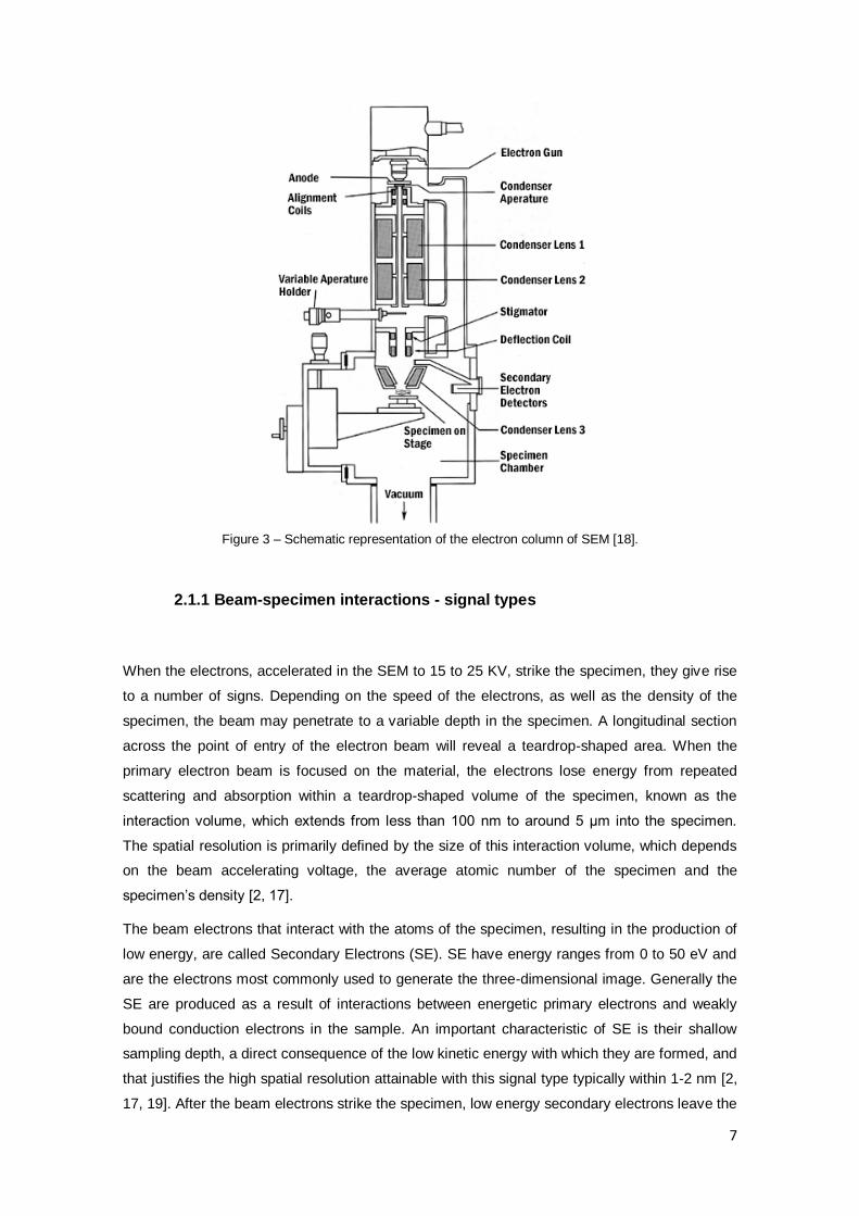
Figure 3 – Schematic representation of the electron column of SEM [18].

2.1.1 Beam-specimen interactions - signal types

When the electrons, accelerated in the SEM to 15 to 25 KV, strike the specimen, they give rise

to a number of signs. Depending on the speed of the electrons, as well as the density of the

specimen, the beam may penetrate to a variable depth in the specimen. A longitudinal section

across the point of entry of the electron beam will reveal a teardrop-shaped area. When the

primary electron beam is focused on the material, the electrons lose energy from repeated

scattering and absorption within a teardrop-shaped volume of the specimen, known as the

interaction volume, which extends from less than 100 nm to around 5 μm into the specimen.

The spatial resolution is primarily defined by the size of this interaction volume, which depends

on the beam accelerating voltage, the average atomic number of the specimen and the

specimen’s density [2, 17].

The beam electrons that interact with the atoms of the specimen, resulting in the production of

low energy, are called Secondary Electrons (SE). SE have energy ranges from 0 to 50 eV and

are the electrons most commonly used to generate the three-dimensional image. Generally the

SE are produced as a result of interactions between energetic primary electrons and weakly

bound conduction electrons in the sample. An important characteristic of SE is their shallow

sampling depth, a direct consequence of the low kinetic energy with which they are formed, and

that justifies the high spatial resolution attainable with this signal type typically within 1-2 nm [2,

17, 19]. After the beam electrons strike the specimen, low energy secondary electrons leave the

8

specimen from many different angles. Because they are weakly negative, the SE will be

attracted to any positive source. The secondary electron detector uses this phenomenon to

gather electrons. The brightness of the SE signal depends on the number of electrons reaching

the detector. If the beam enters the sample perpendicularly to the surface, then the activated

region is uniform about the axis of the beam and a certain number of SE “escape” from within

the sample. As the angle of incidence increases, the “escape” distance of one side of the beam

will decrease, and more secondary electrons will be emitted. Thus steep surfaces and edges

tend to be brighter than flat surfaces, and this result in topographical images with well-defined,

three-dimensional appearance [2, 17].

Backscattered Electrons (BSE) are high-energy electrons and can escape from a much larger

volume than SE. This type of scattering occurs when a beam electron collides with, or passes

close to, the nucleus of an atom of the specimen. The intensities of the different types of signal

depend on the average atomic number of the specimen, but are less dependent on topography.

BSE images have lower spatial resolution than SE images due to the larger volume of their

origin, but can show contrast between areas with different chemical compositions, since the

signal intensities increase with the average atomic number in the sample [2, 17].

2.1.2 Energy Dispersive Spectroscopy and X-ray mapping

Energy Dispersive X-ray Spectroscopy (EDS) is a standard technique for element identification

in material analysis. EDS systems are mounted on SEM and use the primary beam of the

microscope to generate characteristic X-rays. The composition of the sample is found by

analyzing the energy of the characteristic X-rays. The spatial resolution of EDS depends on the

sample material and the energy of the primary beam of the SEM [19]. When the sample is

bombarded by the SEM's electron beam, electrons are ejected from the atoms comprising the

sample's surface. The resulting electron vacancies are filled by electrons from a higher state,

and an X-ray is emitted to balance the energy difference between the two electrons' states. The

X-ray energy is characteristic of the element from which it was emitted. The EDS X-ray detector

measures the relative abundance of emitted X-rays in relation to their energy. The detector is

typically a lithium-drifted silicon, solid-state device [19, 20].

A qualitative analysis is possible: the sample X-ray energy values from the EDS spectrum are

compared with known characteristic X-ray energy values to determine the presence of an

element in the sample. Elements with atomic numbers ranging from that of Beryllium to Uranium

can be detected.

It is possible to obtain an elemental mapping (X-ray mapping): characteristic X-ray intensity is

measured relative to lateral position on the sample. Variations in X-ray intensity at any

characteristic energy value indicate the relative concentration for the applicable element across

the surface. One or more maps are recorded simultaneously using image brightness intensity

9

as a function of the local relative concentration of the element(s) present. About 1 μm lateral

resolution is possible [20].

In this present work, Scanning Electron Microscopy observations in BSE modes, as well as X-

ray mapping were carried out with a Hitachi S-2400 microscope operated at 25 kV and

equipped with a standard Rontec EDS detector. The SEM work consisted of an observation of

the polished sialolith cross-section to obtain structural and chemical information.

2.1.3 Sample preparation

The specimen (Sialolith 1) was embedded in an epoxy resin by cold mounting. After a

polymerization period of 24 hours the non-embedded part of the sample (Sialolith 1b) was cut

and kept for subsequent TEM observation (Figure 4). Special care was put into this operation to

avoid contamination of the sample. The resin-embedded cross-section was grounded with SiC

paper and polished using alumina suspensions in water.

Figure 4 – Embedding procedure yielding a mounted sample, which was subsequently polished and used

for an SEM observation. The non-embedded part subjected to the TEM [2].

The polished sample (Sialolith 1a) was mounted in metallic supports and coated with carbon in

a Polaron E-5100 coating unit prior to observation to prevent charge accumulation.

10

2.2 Transmission Electron Microscopy

Transmission electron microscope is an analytical tool that allows detailed investigation of the

morphology, structure and local chemistry of metals, ceramics, polymers, biological material and

minerals. It also enables the investigation of crystal structures, crystallographic orientations

through electron diffraction, as well as second phase precipitates’ and contaminants’

distributions by EDS. Magnifications of up to 500,000x and detailed resolutions below 1 nm are

achieved routinely. Quantitative and qualitative elemental analysis can be provided from

features smaller than 10 nm [16].

The instrument includes an electron gun which emits electrons into the vacuum and accelerates

them between the cathode and anode. The most common types of TEM have thermionic guns

capable of accelerating the electrons through a selected potential difference in the range 60 to

120 kV. Schottky-emission and field emission guns are newer alternatives for which the energy

spread is less and the gun brightness higher. The condenser lens system of the microscope

controls the specimen illumination, which ranges from uniform illumination of a large area at low

magnification, through a stronger focusing for high magnification. TEM specimen stage designs

include airlocks to allow for the insertion of the specimen holder into the vacuum with a minimal

increase in pressure in other areas of the microscope. The specimen holders are adapted to

hold a standard size of grid upon which the sample is placed. The standard TEM grid size is a

3.05 mm diameter ring, with a thickness and mesh size ranging from a few to 100 μm. The

sample is placed onto the inner meshed area which has a diameter of approximately 2.5 mm.

The grid is typically made of copper, except when analytical methods are employed and in this

case it can be made of molybdenum, gold or platinum and is placed into the sample holder.

Observation of the images on a fluorescent screen, and the recording of image on photographic

emulsions are currently replaced by techniques that allow digital, parallel, and quantitative

recording of the image intensity [21, 22].

2.2.1 Imaging techniques

Bright Field imaging is used for the examination of most ultrastructures. In order to examine

samples in Bright Field, the objective aperture must be inserted (Figure 5). The objective

aperture is a metal plate with holes of various sizes drilled into it. The aperture is inserted into

the back focal plane, the same plane at which the diffraction pattern is formed. The back focal

plane is located just below the sample and the objective lens. When the aperture is inserted, it

only allows the electrons in the transmitted beam to pass and contribute to the resulting Bright

Field image. When an electron beam strikes a sample, some of the electrons pass directly

through, while others may undergo slight inelastic scattering from the transmitted beam. The

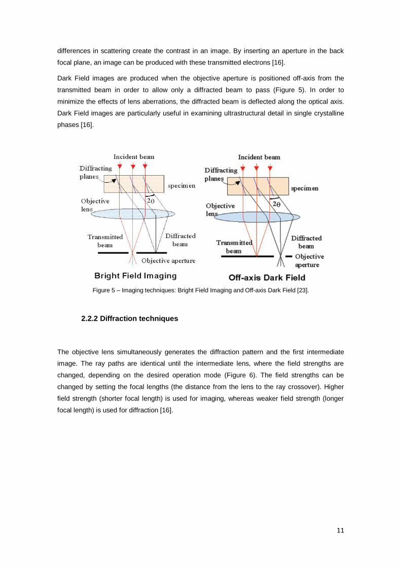
11

differences in scattering create the contrast in an image. By inserting an aperture in the back

focal plane, an image can be produced with these transmitted electrons [16].

Dark Field images are produced when the objective aperture is positioned off-axis from the

transmitted beam in order to allow only a diffracted beam to pass (Figure 5). In order to

minimize the effects of lens aberrations, the diffracted beam is deflected along the optical axis.

Dark Field images are particularly useful in examining ultrastructural detail in single crystalline

phases [16].

Figure 5 – Imaging techniques: Bright Field Imaging and Off-axis Dark Field [23].

2.2.2 Diffraction techniques

The objective lens simultaneously generates the diffraction pattern and the first intermediate

image. The ray paths are identical until the intermediate lens, where the field strengths are

changed, depending on the desired operation mode (Figure 6). The field strengths can be

changed by setting the focal lengths (the distance from the lens to the ray crossover). Higher

field strength (shorter focal length) is used for imaging, whereas weaker field strength (longer

focal length) is used for diffraction [16].

12

Figure 6 – Comparison between imaging mode and diffraction mode [23].

Electron diffraction was used to produce ring patterns of crystalline material in sialolith. This

type of pattern is created when electron diffraction occurs simultaneously from many grains with

different orientations relative to the incident electron beam. Ring patterns can be used to identify

unknown phases or characterize the crystallography of a material. The radii and spacing of the

rings are governed by [16]:

(1)

Where is the interplanar spacing, is the ring radius, and is known as the camera constant.

2.2.3 Sample preparation (Ultramicrotomy)

It is not straight-forward to make a specimen thin enough for TEM (from a few tenths of a

nanometre, to a micron in thickness). The task is made harder still by the need to avoid

changes in the specimen due to the preparation technique, and to obtain a representative

region. The sample must also be strong enough to handle, and last at least long enough to be

13

examined in the microscope [22]. Specimen preparation techniques can be divided into two

basic approaches. First: the removal of unwanted material, by either chemical or mechanical

means, until only a very thin specimen is left behind. Second: cutting the sample is either cut

with a knife or cleaving along crystallographic planes so that a very thin specimen, or region of a

specimen, is produced [22]. In this present work the second was used: the material was cut with

a knife using an ultramicrotome. An ultramicrotome is a slicing instrument developed from the

larger-scale devices used for cutting tissue sections for biological materials. In an

ultramicrotome a firmly mounted or embedded specimen with an area less than 1 mm x 1mm is

moved past a fixed knife made of diamond (Figure 7). The resulting slices are collected in a

liquid-filled trough and are mounted on grids before being inserted into the microscope [22]. In

this present work, specimens needed to be embedded in epoxy resin before sectioning, in order

to provide support during cutting.

Figure 7 – Ultramicrotomy using a diamond knife [24].

The samples used for TEM observation were cut from Sialolith 1b. Two types of samples were

prepared, calcified and decalcified. To obtain these samples the following steps were

performed:

Part of the Sialolith 1b was fractured into small pieces.

For decalcification some fragments were immersed in EDTA at 25% in glutaraldehyde

0.1 M at 3%, pH 7.2 for approximately one month, changing the solution every two days

until the solution becomes translucent. After this procedure were decalcified and two

fixative procedures were necessary. The first fixation was carried out with

glutaraldehyde 3% in sodium cacodylate 0.1 M, pH 7.3. The second fixation was the

immersion in osmium tetroxide 1% in sodium cacodylate to cross-link and stabilize cell

and organelle membrane lipids.

14

For the calcified sample, only the fixation (mentioned above) procedure was performed.

Both calcified and decalcified fragments were subsequently dehydrated in ethanol,

followed by embedment in an epoxy resin by cold mounting for 24 hours.

The embedded samples were cut using an Ultramicrotome Reichert.

The samples were stained with uranyl acetate 2% in bidistilled H2O for 20 minutes and

lead citrate (Reynolds) for 4 minutes.

The samples were finally placed on a copper grid with an amorphous carbon

membrane.

The calcified and decalcified samples were both observed using a JEOL - JEM 100 SX TEM

operated at 100kV and by Hitachi H-8100 TEM was operated at 200 kV. Ring diffraction

patterns were obtained with the latter instrument.

15

2.3 Atomic Force Microscopy

The high-resolution images of the AFM are obtained by measuring and controlling the

interaction force between tip and sample. First, a tip at the end of a cantilever approaches the

sample, and then scans over the surface, driven by a piezoelectric actuator (Figure 8). While

scanning, the force between the tip and the sample is measured by monitoring the deflection of

the cantilever. The deflection is detected by a position-sensitive photodiode detector, onto which

the cantilever reflects a laser light. Finally, a topographic image of the sample is obtained by

plotting the defection of the cantilever in relation to its position on the sample [25, 26].

Figure 8 – Schematic of an atomic force microscope [27].

According to the different modes of interaction between tip and sample, the operation modes

could be classified into: non-contact mode, contact mode, and intermittent contact mode. In this

present work contact mode was used. In this mode, the tip remains in contact with the target

sample.

Force Spectroscopy (FS) is used to measure forces of interaction between the probe tip and the

surface sample as a function of their distance. The base of the cantilever is moved slowly in the

vertical-z direction towards the sample surface and retracted again after contact or indentation

(or vice versa). This technique provides information on local elasticity and adhesion force [25].

16

2.3.1 Young’s Modulus and Adhesion Force

From the contact lines of force-displacement curves it is possible to retrieve information on the

elastic–plastic behavior of materials.

In the contact part of force curves, both in the approach and in the retraction stages, the elastic

deformation of the sample can be related to its Young’s modulus. In order to relate the

measured quantities to the Young’s modulus, it is necessary to consider the deformation of the

sample . For elastic deformation it is useful to describe the system by means of a potential

energy [26]:

(2)

Where is the tip-sample interaction potential caused by surface forces, the energy due to

bending of the cantilever, the elastic deformation energy of the sample, is the so-called

sample stiffness (slope values of force-distance curve), the spring constant cantilever, the

deflection of the cantilever at its end and the indentation. In general, it can be written thus

[26]:

(3)

In contact , is the tip-sample distance, and if the system is in equilibrium, also

. Substituting, it obtains:

. (4)

This simple relation shows that the slope of the force-displacement curve is a measure of the

stiffness of the sample. If the sample is much stiffer than the cantilever, that is for then

, whereas when , i.e., when the sample is much more compliant than

the cantilever. This gives also a rule of thumb for the choice of the cantilever spring constant in

experiments dealing with the elastic properties of the sample: if the cantilever spring constant is

much lower than the sample spring constant, the force curve will probe primarily the stiffness of

the cantilever, and not that of the sample [26].

17

The stiffness of the sample is related to its Young’s modulus by:

with

. (5)

Here, and are the Poisson’s ratio and the Young’s moduli of tip and sample,

respectively, the reduced Young’s modulus, and is the tip-sample contact radius.

AFM force-distance curves have become an important method for studying the adhesion force.

Adhesion occurs when retracting the tip from the sample surface. The tip stays in contact with

the surface until the cantilever force overcomes the adhesive tip-sample interaction [26].

In the most general sense adhesion force is a combination of electrostatic force, van der Waals

force, meniscus or capillary force and forces of chemical bond or acid–base interactions. In

many of the AFM studies on adhesion force ( ), conditions were chosen such that the van der

Waals forces were expected to dominate. In this case should be determined by the

Hamaker constants of the AFM probe, the sample and the contact geometry. Quantitative

comparison of such experiments with theoretical predictions is hampered by several factors:

Surface roughness has a pronounced influence on adhesion force that is hard to quantify; the

precise contact geometry is often hard to determine and adsorption of contaminants on high

energy solid surfaces leads to chemical inhomogeneities of the surfaces [26]. The adhesion

force can be calculated from the force-distance curve and it is represented in Figure 9.

Figure 9 - Schematic position sensitive detector current signal ( ) vs. piezo position ( ) curve

including approaching and retracting parts. Three types of hysteresis can occur: In the zero force line (A),

in the contact part (B) and adhesion (C) [26].

18

Variations in the shape of force curves taken at different locations indicate variations in the local

nano-scale properties of the specimen surface. The shape of the curve is also affected by

contaminants and surface lubricants, as well as the water content of the surface layer of the

specimen when operating an AFM in air [28].

Topographic images of regions mapped by SEM and X-ray maps were obtained under contact

mode in specific areas of Sialolith 1a (polished cross-section). FS was used to obtain force-

distance curves at selected points of the sample, enabling the assessment of the variations of

the adhesion force and Young’s modulus. AFM/FS work was performed at room temperature

and humidity with a Veeco DI CP-II Atomic Force Microscope using commercially available

silicon cantilevers and coating with Pt/Ir (SCM-PIT, Veeco), with a nominal spring constant of

2.5 N/m and a nominal tip radius of 20 nm after sensitivity calibration.

19

2.4 Proteomic analysis

2.4.1 Electrophoresis

Electrophoresis is a simple, rapid, and sensitive analytical tool for separating proteins. An

electric current is passed through a medium containing the target mixture. Each different type of

molecule travels through the medium at a different rate, depending on its electrical charge

and/or size. Acrylamide gel is the most common media for the electrophoresis of proteins. In the

present work, a NuPAGE system was used: the NuPAGE Novex Midi Gel system, which is a

pre-cast polyacrylamide gel system. NuPAGE Novex Midi Gels are used with the NuPAGE Bis-

Tris SDS Buffer System to produce a discontinuous SDS-PAGE system operating at neutral pH.

The neutral pH 7.0 environment of electrophoresis results in the maximum stability of proteins

and gel matrix, providing better band resolution than other gel systems, including the traditional

SDS-PAGE Laemmli system. For many years the Laemmli system has been the standard

method used to perform SDS-PAGE Laemmli-type gels. These gels are useful for a broad

range of protein separations [29, 30].

The NuPAGE Novex Midi Gels consists of NuPAGE Novex Bis-Tris [Bis (2-hydroxyethyl) imino-

tris (hydroxymethyl) methane-HCL] Midi Gels (for separating small to mid-size molecular weight

proteins), NuPAGE LDS (Lithium Dodecyl Sulphate) Sample Buffer, NuPAGE Sample Reducing

Agent and NuPAGE MOPS [3-(N-morpholino) propane sulfonic acid] SDS (Sodium

Dodecylsulfate) Running Buffer for NuPAGE Noves Bis-Tris Midi Gels.

The NuPAGE Bis-Tris discontinuous buffer system involves three ions [30]:

Chloride is supplied by the gel buffer and serves as a leading ion due to its high affinity to the

anode compared to other anions in the system. The gel buffer ions are Bis-Tris and Cl- (pH 6.4).

MOPS serves as the trailing ion. The running buffer ions are Tris, MOPS and dodecylsulfate (pH

7.3-7.7).

Bis-Tris is the common ion present in the gel buffer and running buffer. The combination of a

lower pH gel buffer (pH 6.4) and running buffer (pH 7.3-7.7) results in a significantly lower

operating pH of 7 during electrophoresis.

The hydrophobic tail of the dodecylsulfate in SDS interacts strongly with polypeptide chains and

it is also a detergent that disrupts protein folding. The NuPAGE LDS Sample Buffer is used to

prepare samples for denaturing gel electrophoresis with the NuPAGE Novex Midi Gels, and it is

formulated to reliably provide complete reduction of the disulfides under mild heating conditions

and eliminate any protein cleavage during sample preparation. The NuPAGE Sample Reducing

Agent contains Dithiothreitol (DTT) and prepares samples for reducing gel electrophoresis [29,

30].

20

2.4.2 Sample Preparation

1. Part of Sialolith 2 was broken down mechanically. These samples were kept in EDTA at 25% in

glutaraldehyde 0.1 M at 3% at room temperature for about 6 months for removal of calcified

matrix, changing the solution every two days until the solution became translucent and gel-like.

Then they were kept at 4 oC.

2. Aliquots of 1 ml containing fragments of the sample were removed and centrifuged at 14000 Xg

for about 15 minutes.

3. The sediments were re-suspended in 50 l of supernatant and diluted 1:2 in NuPAGE sample

buffer (2X) with LDS and a reducing agent. Then they were denatured by heating at 70 °C for

10 minutes, and afterwards they were subjected to electrophoresis.

2.4.3 Electrophoretic analysis

1. The samples were analysed in NuPAGE Novex Bis-Tris gradient gels (4-12%) with NuPAGE

MOPS SDS running buffer, to which a reducing agent was added Gels with 20 wells were

loaded with samples of 25 μl.

2. The electrophoiresis was then processed in a XCell4 SureLock midi cell system at 200 volts for

55 minutes. A sample of a molecular marker (Novex Sharp protein standard) was run in the

same gel.

3. At the end of the procedure, the cassette containing the gel was dismantled and the gel placed

in a box of appropriate size, to be equilibrated in ultrapure water for 30 minutes with shaking.

The gel was then stained with Bio-Safe Coomassie Stain for 1 hour. The dye was replaced by

ultrapure water, which kept the gel preserved until further use.

2.4.4 Processing of the polypeptide bands for sequencing

1. The polypeptide bands visualized on the gel were excised in order to be sent for identification.

The excision was achieved by placing the gel on a transilluminator, the surface of which was

cleaned with 70 % ethanol. To avoid contamination it was necessary to use a disposable sterile

scalpel for each band. It was also necessary to work carefully with gloves, and to have hair

covered with a cap, in order to prevent contamination of skin and hair.

2. The excised protein bands were placed in sterile microtubes and were sent to the Mass

Spectrometry Laboratory, Analytical Services Unit, Instituto de Tecnologia Química e Biológica,

Universidade Nova de Lisboa, in order to be identified. There they were subjected to proteolytic

digestion with trypsin. The peptides resulting from this digestion were purified, concentrated and

21

eluted directly onto a MALDI plate. The mass spectra of the different peptides were obtained

using a MALDI-TOF/TOF MS instrument. MS and MS/MS spectra obtained were analyzed using

a combined of the Mascot search engine and database of NCBI.

22

3. Results and Discussion

3.2. Scanning Electron Microscopy

The use of SEM, in the BSE imaging mode, resulted in the formation of images of the polished

cross-section (Sialolith 1a). X-ray maps of the images show the elements present in the bright

and dark regions.

Figure 10 displays the polished cross-section (Sialolith 1a) with some highlighted details, which

are discussed in this section. The sialolith exibits one central core, which has an irregular shape

and is surrounded by layers.

Figure 10 - Polished cross-section of Sialolith 1a (BSE mode).

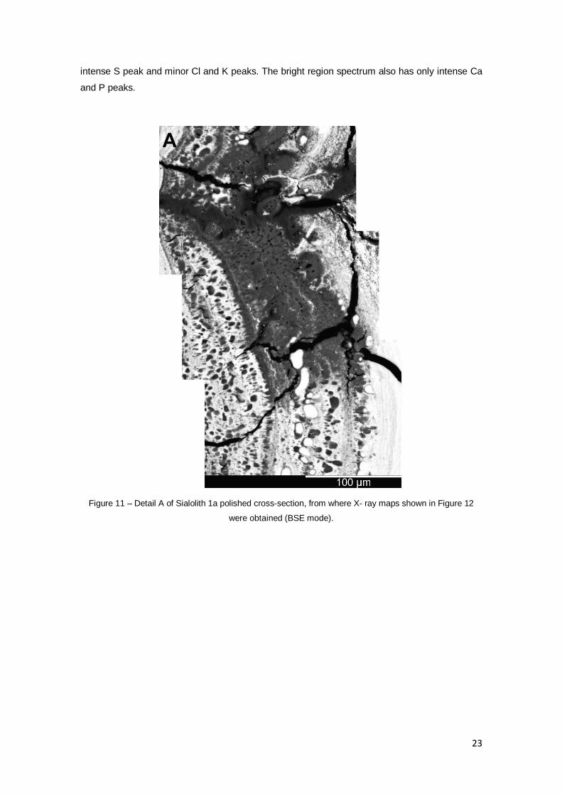
X-ray maps (Figure 12) were made of detail A (Figure 11). These prove that, in the images

produced in the BSE imaging mode, the bright regions are Ca and P-rich and that darker

regions contained S. Typical EDS spectra obtained by Olga Santo [2] from both dark and bright

regions are shown in Figure 13. The dark region spectrum contains peaks of Ca and P, an

23

intense S peak and minor Cl and K peaks. The bright region spectrum also has only intense Ca

and P peaks.

Figure 11 – Detail A of Sialolith 1a polished cross-section, from where X- ray maps shown in Figure 12

were obtained (BSE mode).

24

Figure 12 – (a), (b) and (c) are the Ca, P and S X-ray maps respectively of detail A of the Sialolith 1a

polished cross-section (BSE mode).

Figure 13 – Typical EDS spectra obtained at (a) bright and (b) dark regions [2].

25

Detail B shows part of the core (highly mineralized) with organic teardrop globules (organic

matter) and spherical globules (partially mineralized) (Figure 14). Figure 15 displays layers of

mineralized and weakly mineralized globule convolutions.

Figure 14 – Detail B of the Sialolith 1a polished cross-section display the highly mineralized core.

The arrows indicate the teardrop globules.

Figure 15 – Detail B of the Sialolith 1a polished cross-section. Parts (a) and (b) are convolutions

of mineralized and weakly mineralized globule layers.

26

Detail C displays the core surrounded by incomplete layers of organic matter with partially

spherical mineralized globules (Figure 16). Detail D shows partially mineralized globules

surrounded by crescents of smaller teardrop-shaped structures, which are found in the layers

around the core (Figure 17).

Figure 16 – Detail C of the Sialolith 1a polished cross-section displays the core surrounded by an

incomplete layer of organic matter with spherical globules (indicated by the arrow) (BSE mode).

Figure 17 – Detail D of the Sialolith 1a polished cross-section shows (indicated by the arrow) the globules

surrounded by crescents of smaller teardrop-shaped structures (BSE mode).

27

In detail E, close to the peripheral of the sialolith it is possible to observe laminar layers (Figure

18a) and incomplete layers of spherical globules (highly mineralized) intercalated with

incomplete layers of teardrop-shaped globules (weakly mineralized) (Figure 18b).

Figure 18 – Detail E of the Sialolith 1a polished cross-section. (a) Laminar layers (b) layers of teardrop-

shaped (indicated by the uppermost arrow) and spherical globules (indicated by the lowermost arrow)

(BSE mode).

28

From the results it can be inferred that the bright regions are highly mineralized (Ca and P-rich).

Darker regions, which are essentially composed of organic matter, contain S. In summary, the

salivary calculus exhibits a highly mineralized irregular core, in which organic and partially

organic globules are sparsely distributed, or exist in the form of layer convolutions. Around the

core, incomplete layers of organic matter in which partially mineralized spherical globules are

present. These layers are loosely connected to the subsequent layers. The subsequent layers

present either laminar or globular structures [2]. The laminar layers consist of fine mineralized

strata (1-10 μm) intercalated with fine organic strata (1-5 μm) [2, 9]. However, the sialolith also

contains layers of mineralized globules intercalated with layers of organic globules. These layer

types alternate thereafter in succession following a chronologic sequence. Sialolith 1a has a

core surrounded by a globular layer which is in turn surrounded by a laminar layer. Some

sialoliths previously characterized have a core surrounded by a laminar layer, which is

surrounded by an outer globular layer [2, 6, 9].

The teardrop globules do not always have the same morphology in these images, but the 3-D

globule morphologies are close to teardrop shapes, with a circular configuration in transverse

cross-sections and an elongated configuration in longitudinal cross-sections.

In the layers around the core, partially mineralized globules are surrounded by crescents of

smaller teardrop-shaped structures which may be result from a “squeezing process” induced by

pressure build-up [2].

29

3.2 Transmission Electron Microscopy

TEM was used to observe the components present in the sialolith (Sialolith 1b). Figure 19 was

obtained from the decalcified sample. Figure 19a shows only the organic matter present in the

sialolith and Figure 19b displays the presence of globules with a few crystals inside, which were

supposed to be hydroxyapatite (HA), inside that were not possible to remove with the

decalcification operation.

Figure 19 – Decalcified sample. (a) Organic matter without HA crystals, the arrows indicate the

spaces in organic matter where HA crystals were present before decalcification (b) globules (Y) with a few

HA crystals inside, the arrows indicate HA crystals.

30

In the calcified sample it is possible to observe organic globules surrounded by many HA

crystals (Figure 20a) and HA crystals inside the globules (Figure 20b).

Figure 20– Calcified sample. (a) Globules (Y) surrounded by HA crystals in organic matter and (b)

HA crystals inside a globule, the arrows indicate the HA crystals.

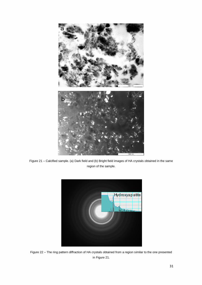
Dark field and Bright field imaging were used to roughly determine the HA crystals size, which

ranged from a few tens to hundreds of nanometres (Figure 21). The presence of HA was

confirmed by indexation of the ring diffraction pattern (Figure 22).

31

Figure 21 – Calcified sample. (a) Dark field and (b) Bright field images of HA crystals obtained in the same

region of the sample.

Figure 22 – The ring pattern diffraction of HA crystals obtained from a region similar to the one presented

in Figure 21.

32

Evidence for bacteria existence was found in the sialolith observed (Figure 23). These bacteria

have thick cell walls and rod-shapes which suggest that they are Gram-positive. Dark field and

Bright field images were also used to observe the HA crystals inside and surrounding the

bacteria (Figure 24).

Figure 23 – Calcified sample with bacteria. (a) and (b) bacteria (B). The arrow point to the occurrence of

cell division of bacteria.

33

Figure 24 – Calcified sample. (a) Dark field and (b) Bright field images of HA crystals inside and

surrounding the bacteria.

These bacteria have thick cell walls and are rod-shaped. The bacteria size is 1 μm

transversely and 1 – 1.5 μm longitudinally. It was possible to detect bacteria in the process of

division. Bacteria grow to a fixed size and then reproduce through binary fission, a form of

asexual reproduction [31]. Bacteria can grow and divide extremely rapidly [32]. The high sulfur

content in the organic matter (previously discussed in section 3.1), might be produced by

bacteria [33]. To the author best knowledge evidence for a possible S origin had not been

previously reported.

Organic matter has an irregular distribution and may be composed of denatured collagen [2].

HA crystals are present inside some of the organic globules structures. A hypothesis for this is

that the mineralization starts with the diffusion of the Ca and P into globule interior, followed by

34

the precipitation of mineralized flakes, which grow or agglomerate inside the globules and

transform during the process into HA [2]. In summary, the results obtained allow to conclude

that the main component of the mineral matter is hydroxyapatite and that bacteria may be an

important factor in sialolith formation.

35

3.3 Atomic Force Microscopy

This work aimed at establishing an experimental protocol for mechanical behaviour assessment

and some preliminary results are presented here. FS was used to obtain force-distance curves

at selected points in specific areas (detail A) of the Sialolith 1a polished cross-section (Figure

11). Through these force-distance curves it is possible to obtain the Young’s modulus and

adhesion force values.

The measurements were carried out in the bright and dark regions corresponding to A and B in

Figures 25 and 26, respectively. Figure 27 displays the topographic images of regions A and B.

Figure 28 shows a typical force-distance curve.

Figure 25 – Region A of detail A of the Sialolith 1a polished cross-section obtained in BSE mode by SEM.

Region A is located in a highly mineralized area.

36

Figure 26 – Region B of detail A of the Sialolith 1a polished cross-section obtained in BSE mode by SEM.

Region B is located in a weakly mineralized area.

Figure 27 – Topographic images of regions A (scan size: 13 μm x 13 μm) and B (scan size: 40 μm x 40

μm) from the polished cross-section. (x) and (y) are points selected in order to obtain force-distance curves

of each region.

37

Figure 28 – Example of the force-distance curve obtained at point x (Figure 21). Force-distance curve

describing a single approach-retract cycle of the AFM tip: (A) The AFM tip is approaching the sample

surface and the long range interactions are too small to give measurable deflections; (B) the initial contact

between the tip and the surface is mediated by attractive Van der Waals forces (contact) that lead to an

attraction of the tip toward the surface; (C) the tip applies a constant and default force upon the surface

that leads to sample indentation, cantilever deflection and increase of repulsive forces; (D) subsequently,

the tip tries to retract and to break loose from the surface; (E) various adhesive forces between the sample

and the AFM tip, however, hamper tip retraction. These adhesive forces can be taken directly from the

force-distance curve; (F) the tip looses contact with the surface upon overcoming of the adhesive forces [2]

is the slope of the force-distance curve. The adhesive force ( ) is the difference between

the snap-in point (the point of contact between the cantilever tip and specimen surface) and the

snap-out point (the point of separation or detachment between the cantilever tip and specimen

surface). Thirty force-distance curves were obtained for each region, (N/m) and mean

values were determined (Table 1).

Table 1 – Mean values of (N/m) and (N), and their standard deviations for the bright and dark

regions.

Bright region (region x)

Dark region (region y)

(N/m) -2.92 ± 7.00 10

-2 -2.90

± 1.32 10

-1

(N) 1.22 10-7

± 7.88 10-8

3.22 10-8

± 1.68 10-8

The mean values were used to calculate the Young’s modulus values presented in Table 2

using the equation (5) and by considering that the Young’s modulus of the silicon tip ( ) is 150

GPa, the nominal tip radius ( ) is 20 nm, and that the Poisson’s ratio of tip to sample (

38

respectively) was considered as 0.3 it was possible to calculate the Young’s modulus of each

region ( ).

Table 2 – Young’s modulus (MPa) for the bright and dark regions

Bright region (region x)

Dark region (region y)

Young’s modulus, (MPa)

66.4 66.0

The AFM results show that the average Young’s modulus of the sialoliths is close to 66 MPa.

Nevertheless, a higher number of curves would be required to differentiate the two regions. The

same applies to the adhesion force values, which exhibited a large dispersion. Indeed a higher

adhesion force would be expected for the dark regions due to higher content of adhesive

substances (may be the presence of collagen) [2]. However since the measurements have been

carried out first in the dark region, contamination of the tip with organic matter may have

influenced the adhesion results.

Figure 29 shows the Young’s moduli of different materials [34]. The sialolith Young’s modulus is

situated between those of gelatin and protein crystals (10 MPa and 120 MPa, respectively). This

means that the sialolith material is very soft and that the hydroxyapatite crystals are not having

a strong reinforcement effect.

Figure 29 - Young’s (elastic) moduli of different materials. The diagram shows a spectrum from very hard

to very soft: steel > bone > collagen > protein crystals > gelatin, rubber > cells [34].

As suggested by Olga Santo [2] some regions of the sialolith showed a fracture surface

characteristic of a ductile material containing hard inclusions. When a material contains

relatively hard inclusions which do not deform at the same rate as the matrix, voids are

nucleated to accommodate this incompatibility. The nucleation involves decohesion at the

inclusion-matrix interface and when a ductile fracture surface is examined, it shows dimples,

39

that correspond to the voids. Therefore the relatively high adhesion forces measured and the

ductile behaviour previously observed may justify the modest success rates obtained by shock-

wave lithotripsy with salivary calculi [8, 9, 35] when compared with renal calculi which contain

less organic material [36].

A protocol for assessment of the mechanical properties of sialolith components has been

established. The Young Modulus and adhesivity of the sialolith can be measured by FS yet care

must be taken so that mineralized regions are probed first in order to minimize the tip

contamination with organic matter.

40

3.4 Proteomic analysis

Several gels were made from the samples and then four bands were selected for analysis by

Mass Spectrometry. These four bands were visible after staining with Coomassie Blue (Bio-Safe

Coomassie Stain, Bio Rad). Two bands had molecular weights exceeding 260 kDa and the

other two bands had molecular weights between 20 and 30 kDa. The two bands weighing 260

kDa had been taken from one gel, whereas the other two bands had been taken from a second

gel. Table 3 and 4 shows the proteins obtained.

Table 3 – Proteins with high molecular weight except Humam Cathepsin G (low molecular weitht) and their

accession number.

Proteins Human Cathepsin G

Crystal Structure Of Human Alpha-

Defensin-4

Medullasin

Acession number

gi|3891975 gi|109156990 gi|233229

Table 4 – Proteins with high molecular weight and their accession number.

Proteins The Complex Of Human Leukocyte

Elastase

Keratin 1 Keratin 10

Acession number

gi|809343 gi|7331218 gi|186629

Cathepsin G and Human Leukocyte Elastase (HLE) (also called Medullasin or Neutrophil

elastase) are serine proteases. Serine protease is a protease (enzymes that cut peptide bonds

in proteins) in which one of the amino acids at the active site is serine. Neutrophilic

polymorphonuclear leukocytes contain specialized azurophil granules which contains the serine

proteases catheptin G and HLE [37, 38]. These proteolytic enzymes are secreted by neutrophils

during inflammation, they destroy bacteria and are capable of degrading a wide variety of

substrates including elastin, collagen and proteoglycans [37-39]. Due to the existence of these

collagen-degrading proteins in a sialolith it is possible that collagen is present in a sialolith in its

denatured form as suggested by the spectroscopy data [2].

Human Alpha-Defensin-4 (DEFA-4), also called as Neutrophil Defensin 4 (ND-4) or Human

Neutrophil Peptided-4 (HNP-4), is a human peptide that is encoded by the DEFA4 gene [40,

41]. HNP-4 belongs to the alpha-defensin family. Alpha-defensins are particularly abundant in

primary (azurophil) granules of neutrophils and its function is antimicrobial activity against

Gram-negative bacteria, and to a lesser extent, also against Gram-positive bacteria and fungi

[40].

41

Keratins are heteropolymeric structural proteins which form intermediate filaments. These

filaments, along with actin microfilaments and microtubules, compose the cytoskeleton of

epithelial cells. Keratin 1 is a member of the type II cytokeratins family. The type II cytokeratins

consist of basic or neutral proteins which are arranged in pairs of heterotypic keratin chains

coexpressed during the differentiation of simple and stratified epithelial tissues. Keratin 10 is a

member of the type I (acidic) cytokeratin family. Epithelial cells almost always coexpress pairs of

type I and type II keratins, and the pairs that are coexpressed are highly characteristic of a

given epithelial tissue [42, 43]. Keratin 1 and 10 were found in the sialolith, which means that

may be keratins are present in epithelial cells of the duct and they are incorporated in the

sialolith.

42

4. Globular Mechanism

The results obtained provide new information on the globular mechanism discussed by Olga

Santo [2]. Using Figure 2 (globular mechanism) it is possible to rewrite some of the stages.

In stage 3, damage occurs to the duct/gland walls, exposing the foreign body/nidus to

connective tissue. At this point it is possible to prove the presence of bacteria. Bacterial

infection develops in the damaged tissue causing an inflammation. As a result of inflammation,

neutrophils appear, destroying the bacteria.

In stages 4 and 5, a foreign body/nidus invades the connective tissue, followed by the scar

tissue. This tissue contains collagen and an extracellular matrix. The collagen may be

synthesized by fibroblast cells which are a constituent of the connective tissue. Collagen in

sialoliths has a denatured form for which cathepsin G and HLE are responsible.

Figure 2 – Schematic drawing representing the globular and sedimentary cycles in the sialoliths formation

mechanism [2].

43

5. Conclusion

The salivary calculi exhibit a mineralized core with organic and partially organic globules. The

core is surrounded by organic matter layers with partially mineralized globules. These layers are

loosely connected to the subsequent layers. These subsequent layers can be made of laminar

or globular structures. The laminar layers consist of fine mineralized strata intercalated with fine

organic strata, whereas the globular structure layers can be either organic or mineralized. The

inorganic matter consists essentially of hydroxyapatite. The organic matter which has an

irregular distribution may be contains proteins and denatured collagen.

The existence of bacteria in the sialolith has been inferred from the results. The high sulfur

content in the organic matter may have been produced by bacteria. The presence of bacteria

proves the existence of a bacterial infection causing inflammation. The existence of neutrophils,

which destroy bacteria and contain proteolytic enzymes that degrade collagen, was also proved.

Keratins were also found in the sialolith, which probably originated from the epithelial cells of the

duct. The results obtain reinforce the validity of the globular mechanism for the formation of

sialoliths previously proposed.

In relation to the mechanical properties assessment, an experimental protocol has been

established. No significant differences in Young’s modulus were detected between the organic

and calcified regions, but the sialolith was found to present a relatively high adhesion force and

a ductile behaviour.

Fundamental knowledge on sialolith formation and experimental sialolith characterization are

essential both for increasing the probability of a successful treatment of patients and to prevent

further future re-occurrences of sialolithiasis. This research has resulted in important information

on salivary calculi, yet further studies will be required in order to develop a deeper knowledge.

44

6. Future work

Existing studies on sialoliths leave much to be known. More proteomic analysis and mechanical

tests on sialoliths are necessary in order to uncover more information on proteins and to

compare mechanical properties which will allow a better understanding of the sialolith formation

mechanism and refinement of the existing proposed models. Our results demonstrate that a

combined Biology and Materials Science interdisciplinary approach is effective for a deeper

understanding of sialolith pathogenesis and etiology.

45

7. Bibliography

[1] Dorland, W. (2007). Dorland’s Medical Dictionary for Health Consumers, Saunders (an

imprint of Elsevier).

[2] Santo, O. L. (2008). Structural and chemical diversity of sialoliths, Master thesis, Instituto

Superior Técnico (IST), Departament of Materials Engineering.

[3] Kasaboğlu, O., Er N., Tümer, C., Akkocaoğlu, M. (2004). Micromorphology of Sialoliths in

Submandibular Salivary Gland: A Scanning Electron Microscope and X-ray Diffraction Analysis.

Journal of Oral Maxillofacial Surgery, 62: 1253-1258.

[4] Hong, K. W., Yang, Y. S. (2003). Sialolithiasis in the sublingual gland. Journal of

Laryngology & Otology, 117: 905-907.

[5] Teymoortash, A., Wollstein, A. C., Lippert, B. M., Peldszus, R., Werner, J. A. (2002).

Bacteria and Pathogenesis of Human Salivary Calculus. Acta Otolaryngol, 122: 210-214.

[6] Teymoortash, A., Buck, P., Jepsen, H., Werner, J. A. (2003). Sialolith crystals localized

intraglandularly and in the Wharton's duct of the human submandibular gland: an X-ray

diffraction analysis. Archives of Oral Biology, 48: 233-236.

[7] Boskey, A. L., Burstein, L. S., Mandel, D. (1983). Phospholipids associated with human

parotid gland sialoliths [short communication]. Archives of Oral Biology. Vol. 28, No. 7, pp. 655-

657.

[8] Ekberg, O., Isacsson, G. (1981). Chemical analysis of the inorganic component of human

salivary duct calculi. Archives of Oral Biology. Vol. 26, pp. 951-953.

[9] Alves de Matos, A. P., Carvalho, P. A., Almeida, A., Duarte, L., Vilar, R., Leitão, J. (2007).

On the structural diversity of sialoliths. Microscopy and Microanalysis, 13 (5): 390-396.

[10] Urban, W., Geisthoff, M. D. (2007). Tecniques for multimodal salivary gland stone therapy.

Operative techniques in Otolaryngology, 18: 332-340.

[11] Capaccio, P., Torretta, S., Pignataro, L. (2009, December). The role of adenectomy for

salivary gland obstructions in the area of sialendoscopy and lithotripsy. Otolaryngologic Clinics

of North America, 42(6): 1161-71.

[12] Nakagawa, Y., Ahmed, M., Hall, S. L., Deganello, S., Coe. F. L. (1987, June). Isolation from

human calcium oxalate stones of nephrocalcin, a glycoprotein inhibitor of calcium oxalate

crystal growth. Journal of Clinical Investigation. Vol. 79, 1782-1787.

[13] Escudier, M. P., Brown, J. E., Drage, N. A., McGurk, M. (2003). Extracorporeal shockwave

lithotripsy in the management of salivary calculi. British Journal of Surgery. 90: 482-485.

46

[14] Koch, M., Zenk, J., Iro, H. (2009, December). Algorithms for treatment of salivary gland

obstructions. Otolaryngologic Clinics of North America, 42(6): 1173-92.

[15] Goldstein, J., Newbury, D. E., Joy, D. C., Echlin, P., Lyman, C. E., Lifshin, E., et. al. (2003,

January). Scanning electron microscopy and x-ray microanalysis, Vol. 1 (3rd

ed.) Germany:

Springer.

[16] Williams, D. B., Carter, C. B. (1996). Transmission Electron Microscopy: A Textbook for

Materials Science, Vol.4 (1st Ed.) New York: Plenum Press.

[17] Bozzola, J. J., Russell, L. (1998). Electron microscopy: principles and techniques for

biologists (2nd

Ed.). London: Jones & Bartlett Learning.

[18] Central Microscopy. http://www.uiowa.edu/~cemrf/methodology/sem/index.htm, (last

accessed October 2010).

[19] Holleritha, C., Wernicke, D., Bühler, M., Feilitzsch,F., Huber, M., Hӧhne, J. et. al. (2004).

Energy dispersive X-ray spectroscopy with microcalorimeters. Nuclear Instruments and

Methods in Physics Research A 520: 606-609.

[20] Material Evaluation and Engineering, Inc. http://mee-inc.com/eds.html, (last accessed

October 2010).

[21] Reimer, L., Kohl, H. (2008). Transmission electron microscopy: physics of image formation

(5 Ed.) Germany: Springer.

[22] Goodhew, P. J., Humphreys, F. J., Beanland, R. (2001). Electron microscopy and analysis

(3rd

Ed.). New York: Taylor & Francis Group.

[23] Transmission Electron Microscope.

http://www.mete.metu.edu.tr/pages/tem/TEMtext/TEMtext.html, (last accessed October 2010).

[24] Washington University in St. Louis. http://presolar.wustl.edu/work/instrumentation.html, (last

accessed October 2010).

[25] Braga, P., Ricci, D. (2004). Atomic force microscopy: biomedical methods and applications.

Totowa, New Jersey: Humana Press Inc.

[26] Butt, H., Cappella, B., Kappl, M. (2005, August). Force measurements with the atomic force

microscope: Technique, interpretation and applications. Surface Science Reports, 59:1–152.

[27] Michigan Tech. http://nano.mtu.edu/afm.htm, (last accessed October 2010).

[28] Fawzy, A., Farghaly, A. M. (2009). Probing nano-scale adhesion force between AFM and

acid demineralized intertubular dentin: Moist versus dry dentin. Journal of Dentistry, 37: 963-

969.

[29] Invitrogen. www.invitrogen.com, (laste accessed August 2010).

[30] Manual of NuPAGE Novex Midi Gel System (2005). Invitrogen Corporation.

47

[31] Koch, A. (2002). Control of the bacterial cell cycle by cytoplasmic growth. Critical Reviews

in Microbiology, 28 (1): 61–77.

[32] Eagon, R. G. (April 1962). Pseudomonas natriegens, a marine bacterium with a generation

time of less than 10 minutes. Journal of Bacteriology, 83 (4): 736–7.

[33] Washio, J., Sato, T., Koseki, T., Takahashi, N. (2005). Hydrogen sulfide-producing bacteria

in tongue biofilm and their relationship with oral malodour. Journal of Medical Microbiology, 54:

889-895.

[34] Alonso, J. L., Goldmann, W. H. (2002). Feeling the forces: atomic dorce microscopy in cell

biology. Life Sciences, 72: 2553-2560.

[35] Eggers, G., Chilla, R. (2005). Ultrasound guided lithotripsy of salivary calculi using an

electromagnetic lithotripter. Journal of Oral Maxillofacial Surgery, 34: 890-894.

[36] Kaneko, K., Yamanobe, T., Nakagomi, K., Mawatari, K., Onoda, M., Fujimori, S. (2003).

Proteomic in renal research. Analytical Biochemistry, 324: 191-196.

[37] Sinha, S., Watorek, W., Karr, S., Giles, J., Bode, W., Travis, J. (1987). Primary structure of

human neutrophils elastase, Proceedings of the National Academy of Science. Vol. 84, pp.

2228-2232.

[38] UniProt, http://www.uniprot.org/uniprot/P08246, (last accessed September 2010).

[39] Bode, W., Wei, A., Huber, R., Meyer, E., Travis, J., Neumann, S. (1986). X-ray crystal

structure of the complex of human leukocyte elastase (PMN elastase) and the third domain of

the turkey ovomucoid inhibitor. The EMBO Journal. Vol. 5, no.10, pp. 2453-2458.

[40] UniProt, http://www.uniprot.org/uniprot/P12838, (last accessed September 2010).

[41] Wilde, C. G., Griffith, J., Marra, M., Snable, J., Scott, R. (1989). Purification and

Characterization of Human Neutrophil Peptide 4, a Novel Member of the Defensin Family.

Journal of Biological Chemistry. Vol. 264, No. 19, pp. 11200-11203.

[42] UniProt, http://www.ncbi.nlm.nih.gov/omim/148080, (last accessed September 2010).

[43] Kierszenbaum, A., L. (2004). Histologia e Biologia Celular: Uma Introdução à Patalogia. Rio

de Janeiro: Elsevier.