characteristics of the east mediterranean dust variability
TRANSCRIPT
Characteristics of the east Mediterranean dust variability on smallspatial and temporal scales
Accepted for publication in Atmospheric Environment
Yuvala,1,∗, Meytar Sorek–Hamera, Amnon Stuppb, Pinhas Alpertb, David M. Brodaya
aDepartment of Civil and Environmental Engineering, Technion, Israel Institute of Technology, Haifa, IsraelbDepartment of Geophysics and Planetary Sciences, Tel-Aviv University, Tel Aviv, Israel
Abstract
The presence of naturally–occurring dust is a conspicuous meteorological phenomenon charac-terised by very high load of relatively coarse airborne particulate matter (PM), which may containalso various deleterious chemical and biological materials. Much work has been carried out tostudy the phenomenon by modelling the generation and transport of dust plumes, and assessmentof their temporal characteristics on a large (>1000 km) spatial scale. This work studies in highspatial and temporal resolution the characteristics of dust presence on the mesoscale (<100 km).The small scale variability is important both for better understanding the physical characteristicsof the dust phenomenon and for PM exposure specification in epidemiological studies. Unsuper-vised clustering–based method, using PM10 records and their derived attributes, was developedand applied to detect the impact of dust at the observation locations of a PM10 monitoring array.It was found that dust may cover the whole study area but very often the coverage is partial. Onaverage, the larger the spatial extent of a dust event, the higher and more homogeneous are theassociated PM10 concentrations. Dust event lengths however, are only weakly associated withthe PM concentrations (Pearson correlation below 0.44). The large PM concentration variabilityduring spatially small events and the fact that their occurrence is strongly correlated with the ele-vation above sea level of the reporting stations (Pearson correlation 0.87, p–value < 10−5) pointsto small scale spatiotemporal dynamics of dust plumes.
Keywords: Cluster analysis, Dust presence detection, Mesoscale character of dust plumes
1. Introduction1
Dust storms originating in the world’s deserts transport particulate matter (PM) from the sources2
to distances of up to thousands of km and may collect along their trajectory additional pollutants3
and allergens (Goudie, 2014). The presence of dust in the earth’s atmosphere is an interesting4
phenomenon that was studied extensively with the goal of improving our understanding of its5
∗Corresponding author. Department of Civil and Environmental Engineering, Technion I.I.T., Haifa 32000. Tel.:+972 4 8292676.
Email address: [email protected] (Yuval)
Preprint submitted to Atmospheric Environment August 17, 2015
formation, transport and characteristics (eg Prospero et al., 2002; Goudie and Middleton, 2006;6
Maghrabi et al., 2011; Israelevich et al., 2012). The health effects of dust raised concerns and7
many studies looked at its possible association with various medical outcomes (eg the recent8
reviews by Karanasiou et al., 2012, Goudie, 2014, and references therein). Most of the studies9
looked at the dust phenomenon variability on a large (>1000 km) spatial scale (Querol et al.,10
2009; Pey at al., 2013) or at one single location (Kocak et al., 2007; Ganor et al., 2009; Mallone11
et al., 2011; Krasnov et al., 2014). To the best of our knowledge, the variability of dust presence12
at the mesoscale has not been looked at to date.13
Many different methods have been utilised for studying airborne dust. Early work usually14
used chemical speciation in order to assess the contribution of natural sources to the total PM15
levels (eg, Ganor et al., 2001; Rodrıguez et al., 2002). Particles with large fractions of Si, Al, Ca16
and other crustal components were attributed to mineral dust. Such methods involve costly and17
tedious analysis of filter data samples. Later studies sought methods that could be employed in a18
cheaper and more efficient manner. Following Escudero et al. (2005), in most cases an array of19
tools is used for the initial identification of dust episodes (Escudero et al., 2007a; Querol et al.,20
2009; Pey et al., 2013). These include back–trajectory analysis, satellite imagery, meteorolog-21
ical maps, and aerosol concentration maps from dust models. Mallone et al. (2011) used light22
detection and ranging (LIDAR) for detection of dust in Rome. The dust contribution is usually23
estimated using various measures of PM10 levels and their difference from some background24
values (Kocak et al., 2007; Escudero et al., 2007b; Querol et al., 2009, Dadvand et al., 2011;25
Mallone et al., 2011; Pey et al., 2013, Krasnov et al., 2014). Ratios of pollutant concentrations26
are used for verification (eg Mallone et al., 2011). In some cases only remote sensing (Zhang et27
al., 2006; Evan et al., 2006) or modelling outputs (Mitsakou et al., 2008; Jimenez-Guerrero et28
al., 2008) were used in dust studies.29
All the above mentioned studies considered dust presence on a daily basis. The qualitative30
nature of the dust identification methods which they used, and the manual work which they re-31
quire, set limits on the spatial and temporal extent of the phenomena which they were able to32
resolve. A daily temporal resolution seems compatible with epidemiological studies as health33
outcome rarely, if at all, are given at a higher resolution. It may also be sufficient for large scale34
studies concerned with dust contributions at the seasonal or annual time scales in a large spatial35
area. However, the turbulence associated with the transport of dust may be of much smaller36
temporal and spatial scales. Understanding the spatiotemporal variability of dust presence re-37
quires a much finer temporal resolution of the relevant data and an adequately spaced array of38
sensors. A scheme utilising those data have to function in an automatic manner. Ganor et al.39
(2009) introduced an algorithm to automatically detect dust presence using half–hourly PM1040
data series. However, their algorithm was calibrated using daily dust observations at a specific41
location. Daily calibration data are too coarse to capture the high temporal variability that Ganor42
et al. (2009) expected to detect. (They assumed, correctly, that dust events may be as short as43
three hours.) Subsequent analysis also found some errors and omissions in the calibration data44
which were not detected during the original work. Moreover, as noted by Ganor et al. (2009),45
their calibration data may not be suitable for use in other locations, as indeed was found later by46
Viana et al. (2010).47
This work explores the spatiotemporal variability of dust presence at the half–hourly temporal48
resolution in an area which is about 250 km by 40 km, using 19 monitoring stations reasonably49
spaced within it. The analyses are based on dust detection scheme that utilises only half–hourly50
PM10 concentration observations and their attributes. Unlike the above mentioned studies, our51
clustering classification scheme does not require calibration information. It is an unsupervised52
2
optimisation scheme (Liao, 2005; Hastie et al., 2009) which looks for hidden features in the data.53
It has been used extensively in the signal processing and pattern recognition fields (Liao, 2005)54
and we show it can be applied in environmental studies like ours which employ time series of55
substantial length.56
2. Study area57
The study area includes the Israeli shoreline and the western slopes of its coastal mountain range58
(see Fig 1). Local anthropogenic PM sources in the area are mainly transportation and large59
industrial plants. Additional major source of fine PM are secondary particulates transported from60
eastern and southern Europe (Asaf et al., 2008). Dust storms transport mineral dust to the region61
from the Sahara and the Arabian peninsula during the winter and the transition seasons. The dust62
contributes significantly to the total PM load (10-20% of the PM10 concentrations; Ganor et al.,63
2009) and there has been increasing interest in its impact on the population’s health (eg Vodonos64
et al., 2014).65
3. Data66
PM monitoring and meteorological data were obtained from the Technion Centre of Excellence67
in Exposure Science and Environmental Health’s air pollution monitoring data archive. The68
database includes all the half–hourly air quality monitoring data observed in Israel from 1997 to69
date. The data pass quality assurance and quality control processing before being released for70
use. The PM10 data used in this work are from standard monitoring stations (ie comply with the71
EU Council Directive 1999/30/EC for protection of human health), with at least 84% complete72
records for the years 2004-2013. The raw data were recorded by a tapered element oscillating73
microbalance (TEOM) devices (Thermo Scientific 1400) that provides a continuous direct mass74
measurement of particle mass. Table 1 provides descriptive statistics of the PM10 records and75
Fig. 1 shows the geographical locations of the stations. Note that the station numbers are ordered76
from south to north and that all the stations except 4 and 13 are within 35 km from the shoreline.77
Most of the stations are at elevations of less than 300 m above sea level. The only exception is78
station 4, located in Jerusalem at 786 m above sea level. Three of the PM10 stations (numbers 9,79
10 and 15) also observe simultaneously PM2.5. Most of the stations observe ambient temperature,80
and wind direction and speed. A few of them also observe relative humidity, barometric pressure81
and insolation.82
Daily synoptic system classification at 12:00 UTC for the eastern Mediterranean during the83
study period 2004-2013 was calculated following Alpert et al. (2004). The method is based84
on a semi–objective classification of geopotential height, temperature and the horizontal wind85
components at the 1000 hPa level. Alpert et al. (2004) defined 19 synoptic systems characteristic86
to the eastern Mediterranean, which can be lumped into six groups: Red Sea Troughs (RST),87
Persian Trough (PT), High to the West (HW), Siberian Highs (SH), Winter Lows (WL) and88
Sharav Low (SL). Detailed description of the synoptic systems and their grouping as well as the89
classification can be found in Alpert et al. (2004).90
3
4. Methods91
4.1. Dust presence detection using cluster analysis92
The major characteristic of naturally–occurring dust is an unusually high PM load. Dust-related93
PM tends to be of the coarser fractions (Kocak et al., 2007) and thus the main variable which we94
used for the detection of dust was the PM10 concentration. For each PM10 monitoring location,95
the half-hourly time points in 2004-2013 were grouped to dust–related or normal points based on96
the PM10 concentration, and the corresponding running maximum and minimum series, as ex-97
plained below. Additional meteorological and air quality variables were also considered but were98
not used in the final classification for three reasons: (a) with the exception of the PM2.5/PM1099
concentration ratio, none of them seems to contribute a considerable power for the clustering100
process beyond what the PM10 concentration and its attributes provide. (b) using additional101
variables, with values in a dynamic range much different than that of the PM10 concentrations,102
requires a normalisation of the values, for which some undesirable arbitrary decision with a very103
large impact on the clustering must be made. (c) using additional variables in the classification104
process would exclude their use for independent assessment of the classification.105
The running PM10 maxima and minima series were calculated such that each element in the106
series is given by yi = ext{xi−q, xi−q+1, · · · , xi+q−1, xi+q}, where x is the PM10 series, 2q + 1 is107
the operation’s window width and ext{ } takes the extremum, either maximum or minimum, of108
a sequence of values. The window width should be related to the mean duration of dust events.109
We used q = 7 time points (3.5 hours) which results in a 7.5 hours window width. Sensitivity110
analysis did not reveal significant differences in the results using 3 ≤ q ≤ 9.111
Cluster analysis divides a set of state vectors into subsets, or clusters, such that members112
of each cluster are more similar in some mathematical sense to each other than to members of113
other clusters. We used for that purpose the K–means clustering method (Liao, 2005). The114
time–dependent state vectors form in our case the three–dimensional data array Zi, i = 1, · · · ,N,115
where the PM10 concentration and the corresponding running maximum and minimum values116
are the components at each time point, and N is the number of half–hourly time points in the117
study period 2004-2013. Our first goal was a partition of the N state vectors into K clusters118
S = S 1, S 2, · · · , S K with centres µi, i = 1, · · · ,K, such that the sum of the within-clusters sum of119
squared distances from the centres is120
arg minS
K∑j=1
∑Z∈S j
||Z − µ j||2 . (1)
We carried this out using the Matlab c© kmeans function (Matlab, 2013). The K–means minimi-121
sation is not guaranteed to arrive at the global minimum and thus the final values of the clusters’122
centres depend on the initial values from which the search for the minimum starts. In our case123
the sensitivity to the initial values was very weak and the corresponding elements of the clusters’124
centres were all within 1% of each other for many trial runs that started with different random125
initial values.126
The decision about the value of K can be made based on various criteria. Using K = 2 did not127
result in the desired partition to dust-related and non–dust time points. In all the stations one of128
the clusters was clearly composed of only dust–related time points (PM10 concentrations above129
500 µgm−3). However, this cluster was very small. The other, much larger, cluster included130
mainly normal time points but also many time points which were obviously dust-related (PM10131
concentrations in the 100s of µgm−3). A common method to decide about an appropriate value for132
4
the number of clusters K is using the very intuitive yet rigorous F statistic, which is the ratio of the133
between–clusters variability to the within–clusters variability (Liao, 2005). The K maximising134
the F statistic is the most desirable one in the pure statistical sense. We found clear maxima in the135
curves of F as a function of K for the data of all the stations (different maximum for each station).136
Using the maximising K, time points classified to different clusters had specific meteorological137
attributes that correspond to known meteorological scenarios with respect to dust presence. A138
few of the clusters were always distinctively dust-related while others were distinctly associated139
with normal conditions (based on their meteorological characteristics, the associated synoptic140
system and their PM10 attributes). However, there were always a cluster or two which could not141
be classified clearly. These clusters were in many cases quite large so their classification as dust–142
related or not could have a very large impact on the subsequent analyses. Hence our final scheme143
used a partition to the very large number of K = 150 clusters in all the stations. Each of these144
clusters happens to be a sub–cluster of the partition based on the F statistic. The classification of145
the clusters to dust or not dust was based on cut–off values for the cluster centre elements. The146
large number of small clusters enabled tagging them as associated with dust or not with a fine147
resolution; the statistical analyses presented later were only very weakly sensitive to the number148
of clusters for K = 100 and above. The cut–off conditions we used were as follows: a cluster149
was define as impacted by dust if (a) the PM10 and maximal PM10 concentrations of its centre150
were above or equal 110 µgm−3 and 250 µgm−3, respectively, or (b) both the PM10 and minimal151
PM10 concentrations of a cluster’s centre were above or equal 110 µgm−3. The cut-off values152
were based on our experience and the general idea underlying the method of Ganor et al. (2009).153
The somewhat arbitrary nature of the cut-off conditions have some impact on the number of154
detected dust time points. However, the spatiotemporal characteristics of the dust phenomenon155
manifested themselves clearly and with minimal sensitivity for a wide range of cut–off values.156
4.2. Dust events157
The cluster analysis considers the input sets Zi with no reference to their temporal order.158
However, in most cases the process resulted in continuous sequences of dust-related time points,159
as can be seen in Figure 2. The intensity of dust presence during certain synoptic systems fluc-160
tuates significantly, resulting sometimes in short dipping of the PM10 concentration to normal161
values, followed by renewed high levels (eg Fig. 2d). In cases where the end of a dust-flagged162
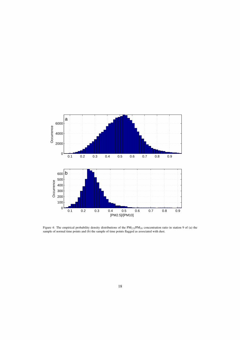
sequence of time points was less than six time points (three hours) from the starting point of the163
next sequence, the time points in between were flagged as dust–related. We refer to continuous164
sequences of time points flagged as dust–related as dust events. Only for comparisons with pre-165
vious studies we refer also to dust days, which we consider to be 24–hours periods, starting at166
00:00, during which dust was detected.167
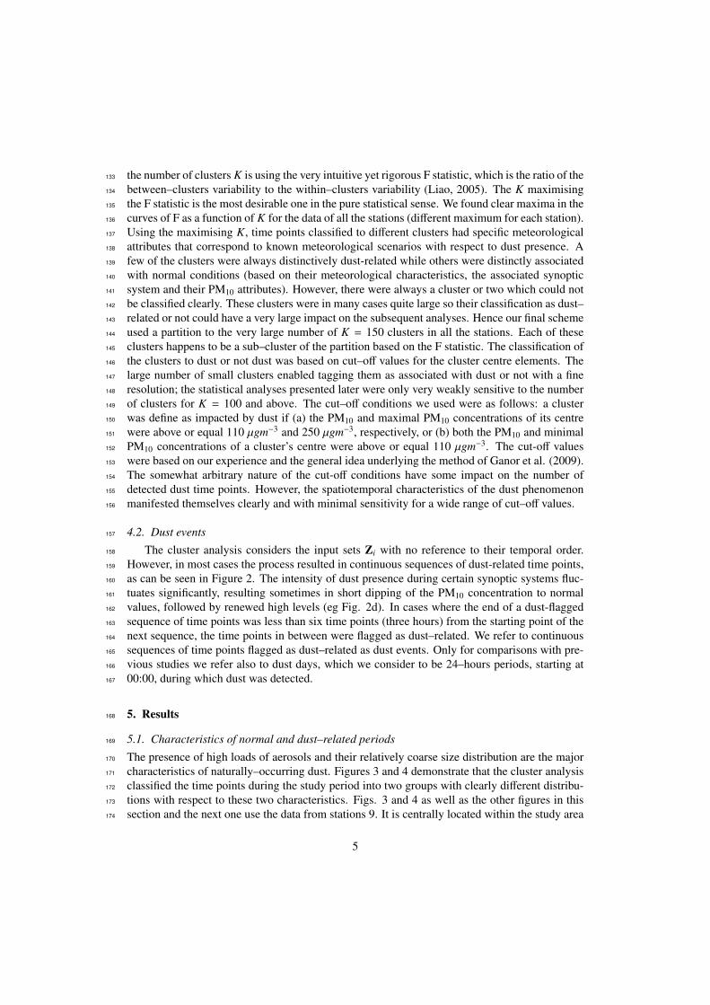
5. Results168
5.1. Characteristics of normal and dust–related periods169
The presence of high loads of aerosols and their relatively coarse size distribution are the major170
characteristics of naturally–occurring dust. Figures 3 and 4 demonstrate that the cluster analysis171
classified the time points during the study period into two groups with clearly different distribu-172
tions with respect to these two characteristics. Figs. 3 and 4 as well as the other figures in this173
section and the next one use the data from stations 9. It is centrally located within the study area174
5
and have records with high completeness for most of the variables. The results for other sta-175
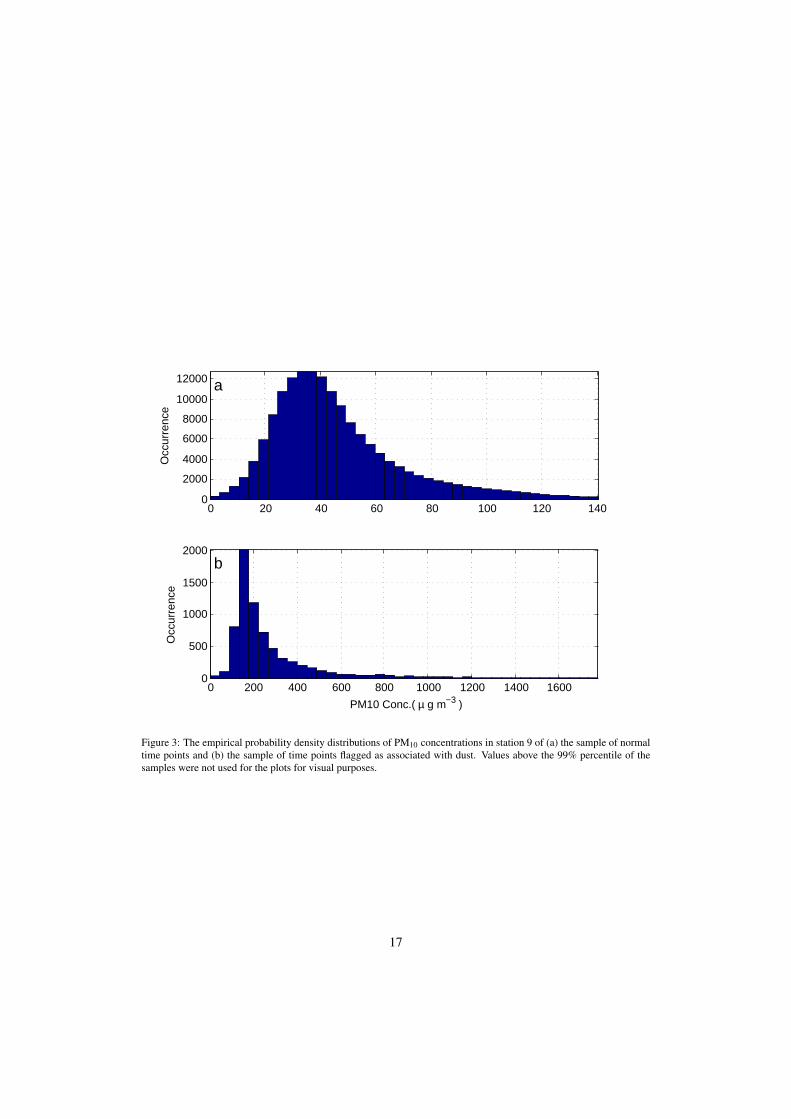
tions are very similar. Figure 3 shows the empirical density distributions of PM10 concentrations176
at normal (non–dust) and dust–related time points. The range of PM10 concentrations during177
non–dust times is between zero and 140 µgm−3, with only 241 (0.14%) of the values above the178
median of the concentrations during dust time points. During time points classified as impacted179
by dust, the PM10 concentrations are up to values above 1600 µgm−3, with only 23 (0.013%) of180
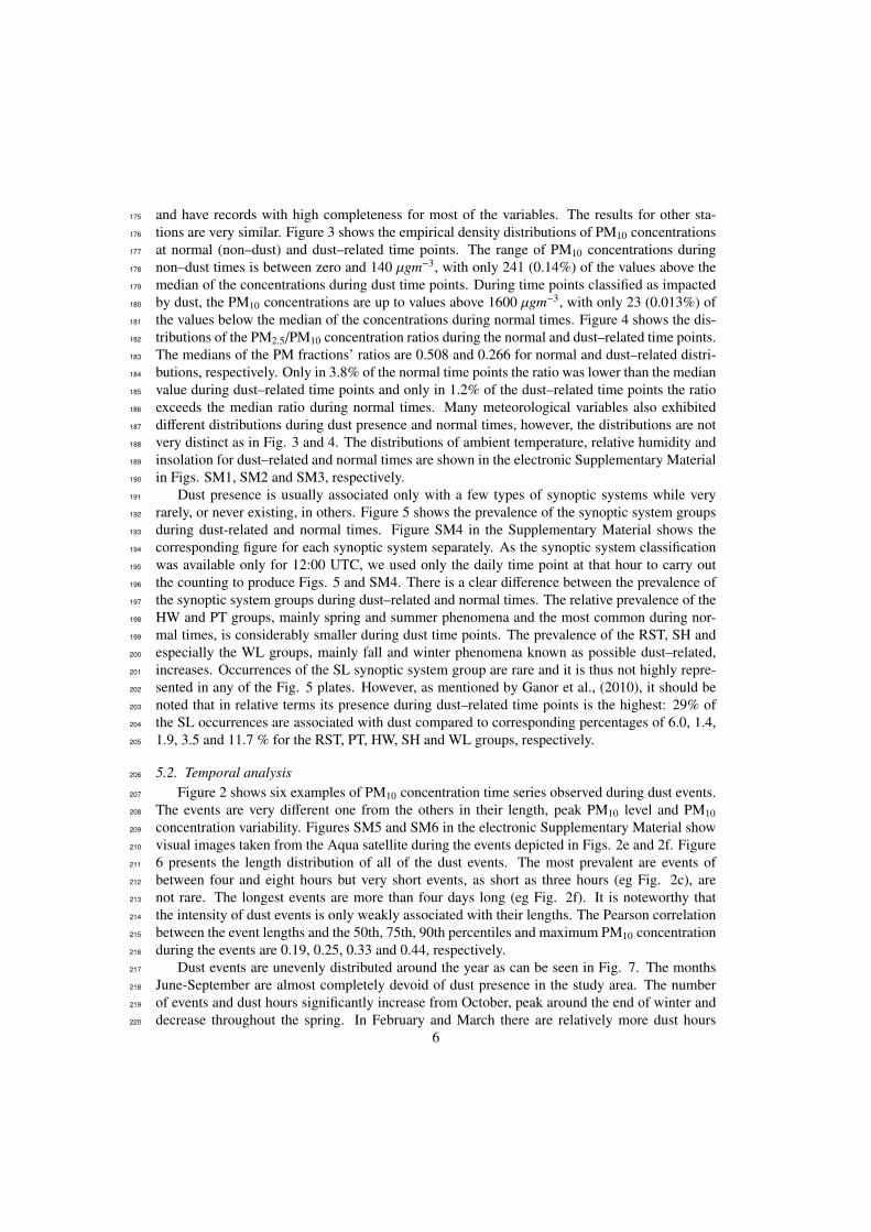
the values below the median of the concentrations during normal times. Figure 4 shows the dis-181
tributions of the PM2.5/PM10 concentration ratios during the normal and dust–related time points.182
The medians of the PM fractions’ ratios are 0.508 and 0.266 for normal and dust–related distri-183
butions, respectively. Only in 3.8% of the normal time points the ratio was lower than the median184
value during dust–related time points and only in 1.2% of the dust–related time points the ratio185
exceeds the median ratio during normal times. Many meteorological variables also exhibited186
different distributions during dust presence and normal times, however, the distributions are not187
very distinct as in Fig. 3 and 4. The distributions of ambient temperature, relative humidity and188
insolation for dust–related and normal times are shown in the electronic Supplementary Material189
in Figs. SM1, SM2 and SM3, respectively.190
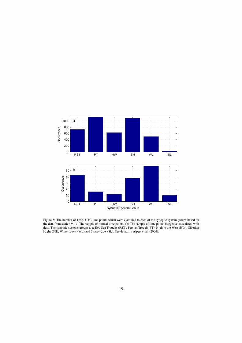
Dust presence is usually associated only with a few types of synoptic systems while very191
rarely, or never existing, in others. Figure 5 shows the prevalence of the synoptic system groups192
during dust-related and normal times. Figure SM4 in the Supplementary Material shows the193
corresponding figure for each synoptic system separately. As the synoptic system classification194
was available only for 12:00 UTC, we used only the daily time point at that hour to carry out195
the counting to produce Figs. 5 and SM4. There is a clear difference between the prevalence of196
the synoptic system groups during dust–related and normal times. The relative prevalence of the197
HW and PT groups, mainly spring and summer phenomena and the most common during nor-198
mal times, is considerably smaller during dust time points. The prevalence of the RST, SH and199
especially the WL groups, mainly fall and winter phenomena known as possible dust–related,200
increases. Occurrences of the SL synoptic system group are rare and it is thus not highly repre-201
sented in any of the Fig. 5 plates. However, as mentioned by Ganor et al., (2010), it should be202
noted that in relative terms its presence during dust–related time points is the highest: 29% of203
the SL occurrences are associated with dust compared to corresponding percentages of 6.0, 1.4,204
1.9, 3.5 and 11.7 % for the RST, PT, HW, SH and WL groups, respectively.205
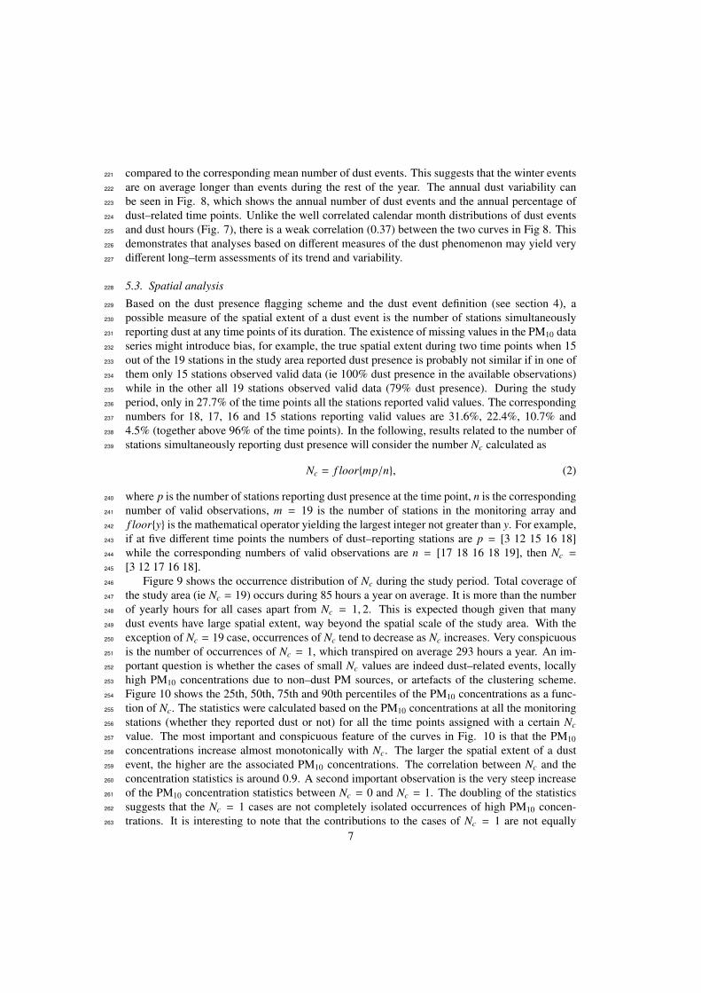
5.2. Temporal analysis206
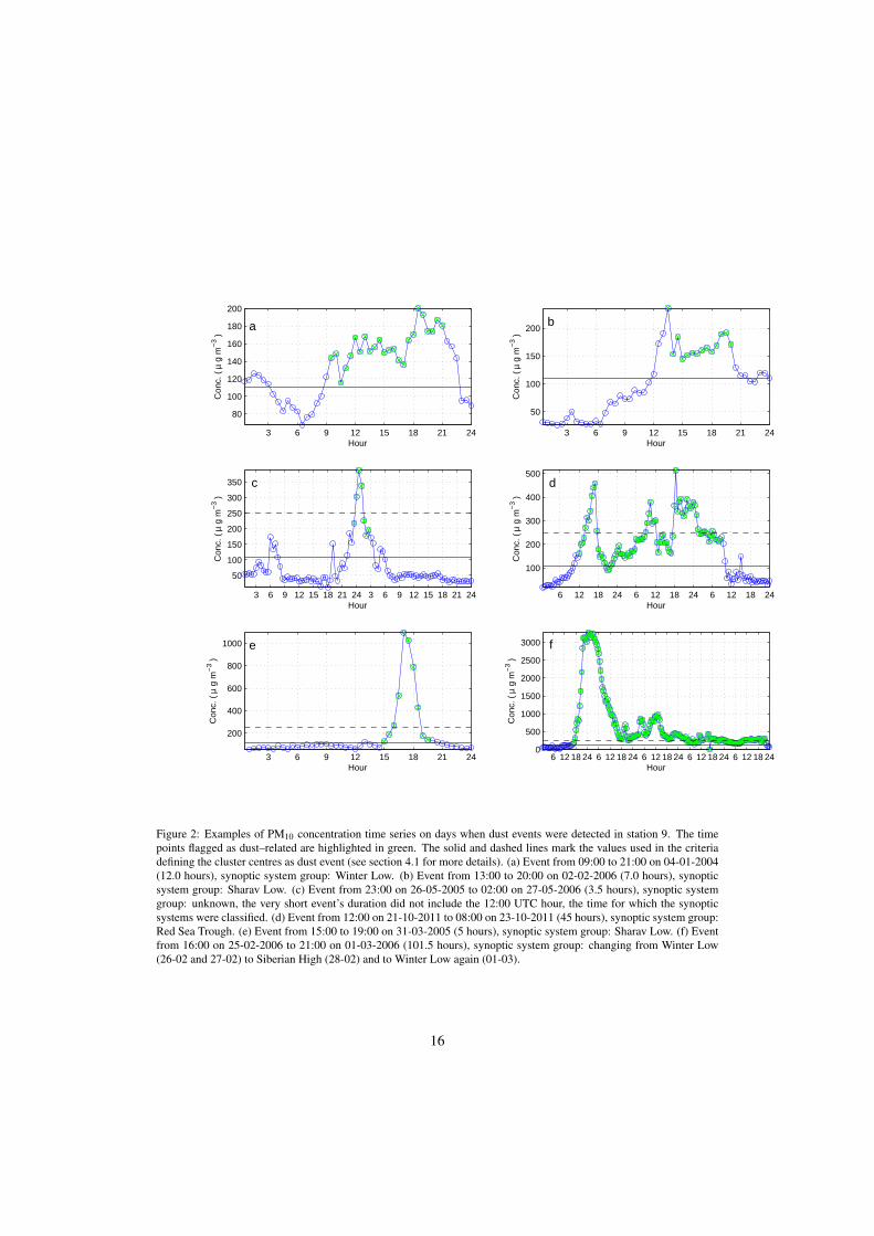
Figure 2 shows six examples of PM10 concentration time series observed during dust events.207
The events are very different one from the others in their length, peak PM10 level and PM10208
concentration variability. Figures SM5 and SM6 in the electronic Supplementary Material show209
visual images taken from the Aqua satellite during the events depicted in Figs. 2e and 2f. Figure210
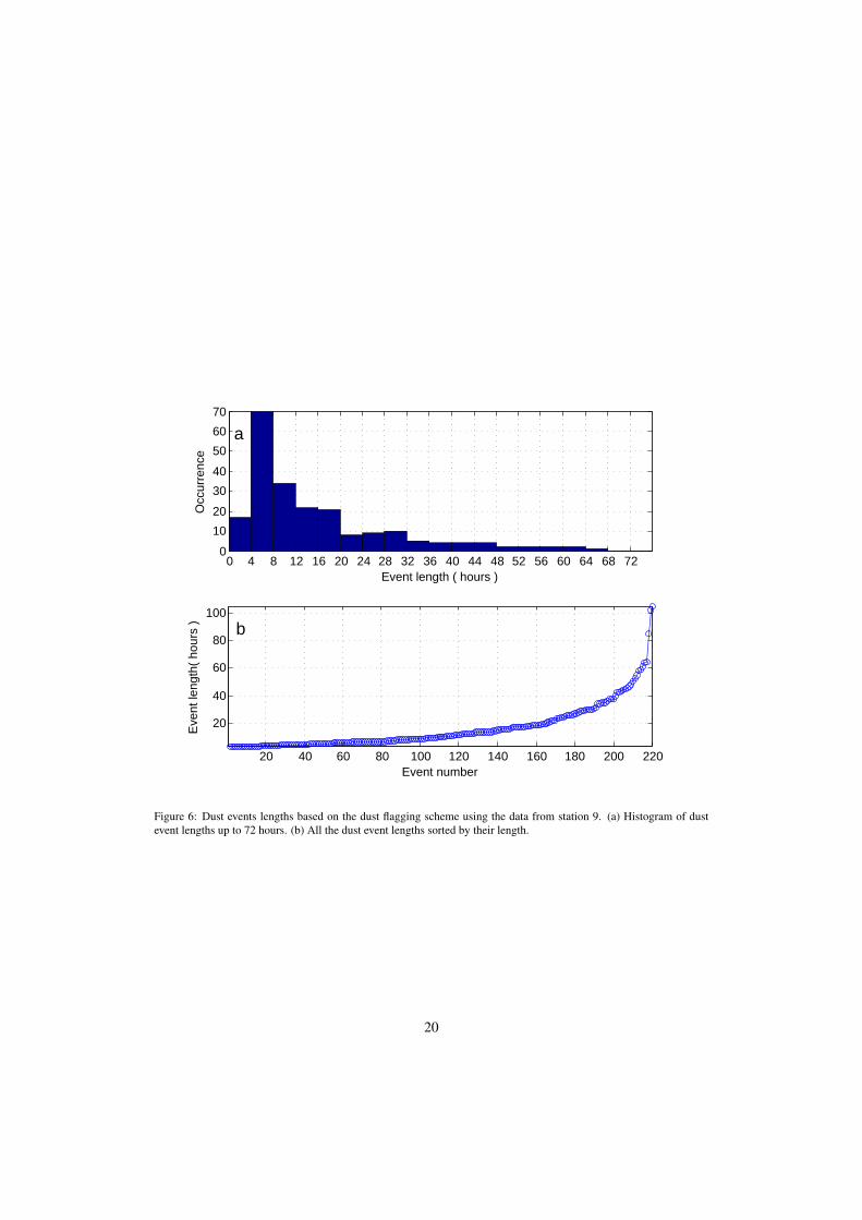
6 presents the length distribution of all of the dust events. The most prevalent are events of211
between four and eight hours but very short events, as short as three hours (eg Fig. 2c), are212
not rare. The longest events are more than four days long (eg Fig. 2f). It is noteworthy that213
the intensity of dust events is only weakly associated with their lengths. The Pearson correlation214
between the event lengths and the 50th, 75th, 90th percentiles and maximum PM10 concentration215
during the events are 0.19, 0.25, 0.33 and 0.44, respectively.216
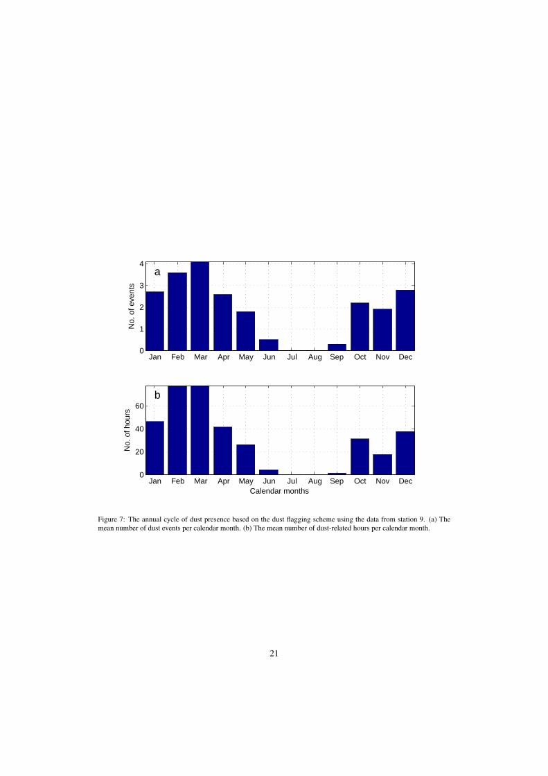
Dust events are unevenly distributed around the year as can be seen in Fig. 7. The months217
June-September are almost completely devoid of dust presence in the study area. The number218
of events and dust hours significantly increase from October, peak around the end of winter and219
decrease throughout the spring. In February and March there are relatively more dust hours220
6
compared to the corresponding mean number of dust events. This suggests that the winter events221
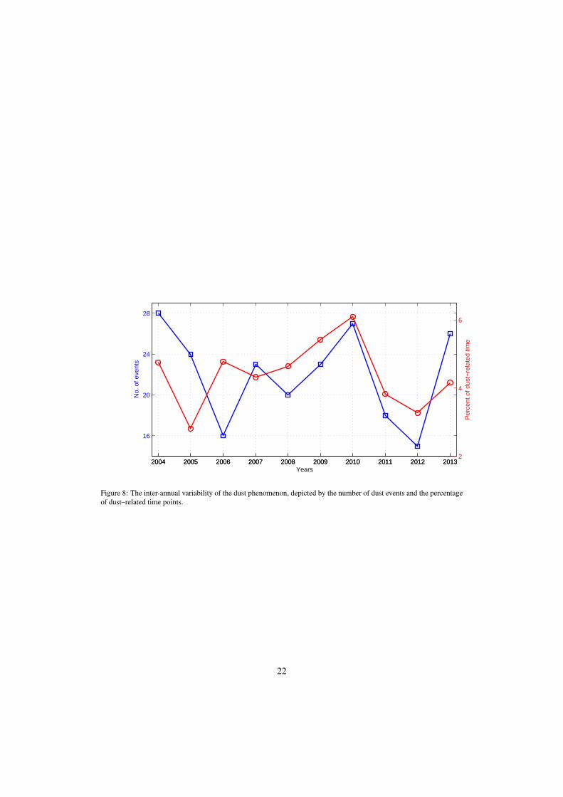
are on average longer than events during the rest of the year. The annual dust variability can222
be seen in Fig. 8, which shows the annual number of dust events and the annual percentage of223
dust–related time points. Unlike the well correlated calendar month distributions of dust events224
and dust hours (Fig. 7), there is a weak correlation (0.37) between the two curves in Fig 8. This225
demonstrates that analyses based on different measures of the dust phenomenon may yield very226
different long–term assessments of its trend and variability.227
5.3. Spatial analysis228
Based on the dust presence flagging scheme and the dust event definition (see section 4), a229
possible measure of the spatial extent of a dust event is the number of stations simultaneously230
reporting dust at any time points of its duration. The existence of missing values in the PM10 data231
series might introduce bias, for example, the true spatial extent during two time points when 15232
out of the 19 stations in the study area reported dust presence is probably not similar if in one of233
them only 15 stations observed valid data (ie 100% dust presence in the available observations)234
while in the other all 19 stations observed valid data (79% dust presence). During the study235
period, only in 27.7% of the time points all the stations reported valid values. The corresponding236
numbers for 18, 17, 16 and 15 stations reporting valid values are 31.6%, 22.4%, 10.7% and237
4.5% (together above 96% of the time points). In the following, results related to the number of238
stations simultaneously reporting dust presence will consider the number Nc calculated as239
Nc = f loor{mp/n}, (2)
where p is the number of stations reporting dust presence at the time point, n is the corresponding240
number of valid observations, m = 19 is the number of stations in the monitoring array and241
f loor{y} is the mathematical operator yielding the largest integer not greater than y. For example,242
if at five different time points the numbers of dust–reporting stations are p = [3 12 15 16 18]243
while the corresponding numbers of valid observations are n = [17 18 16 18 19], then Nc =244
[3 12 17 16 18].245
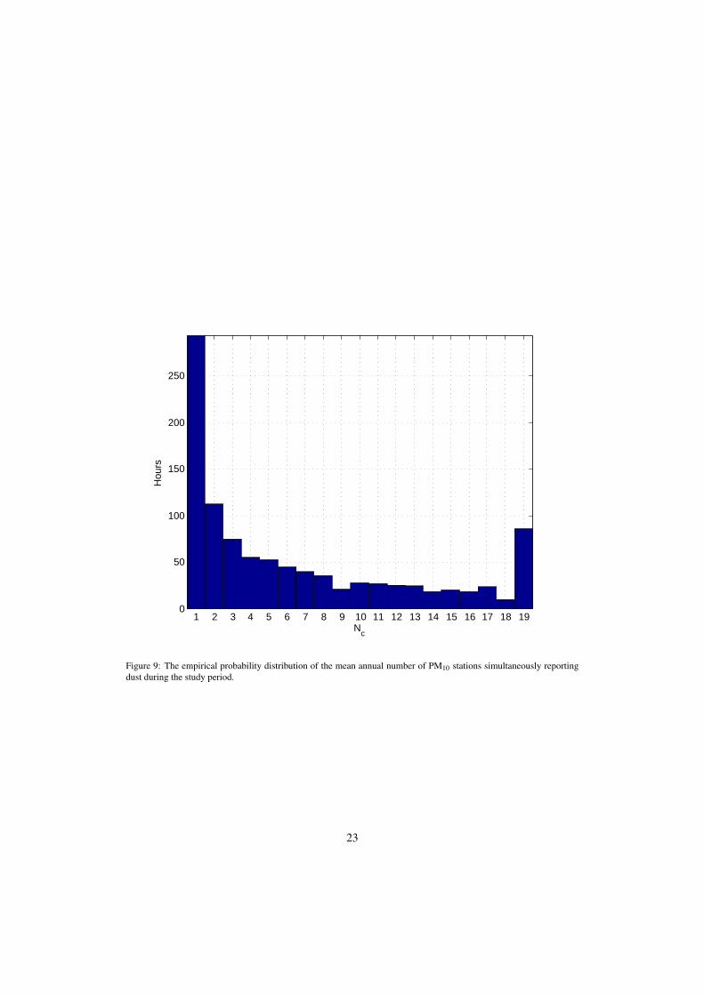
Figure 9 shows the occurrence distribution of Nc during the study period. Total coverage of246
the study area (ie Nc = 19) occurs during 85 hours a year on average. It is more than the number247
of yearly hours for all cases apart from Nc = 1, 2. This is expected though given that many248
dust events have large spatial extent, way beyond the spatial scale of the study area. With the249
exception of Nc = 19 case, occurrences of Nc tend to decrease as Nc increases. Very conspicuous250
is the number of occurrences of Nc = 1, which transpired on average 293 hours a year. An im-251
portant question is whether the cases of small Nc values are indeed dust–related events, locally252
high PM10 concentrations due to non–dust PM sources, or artefacts of the clustering scheme.253
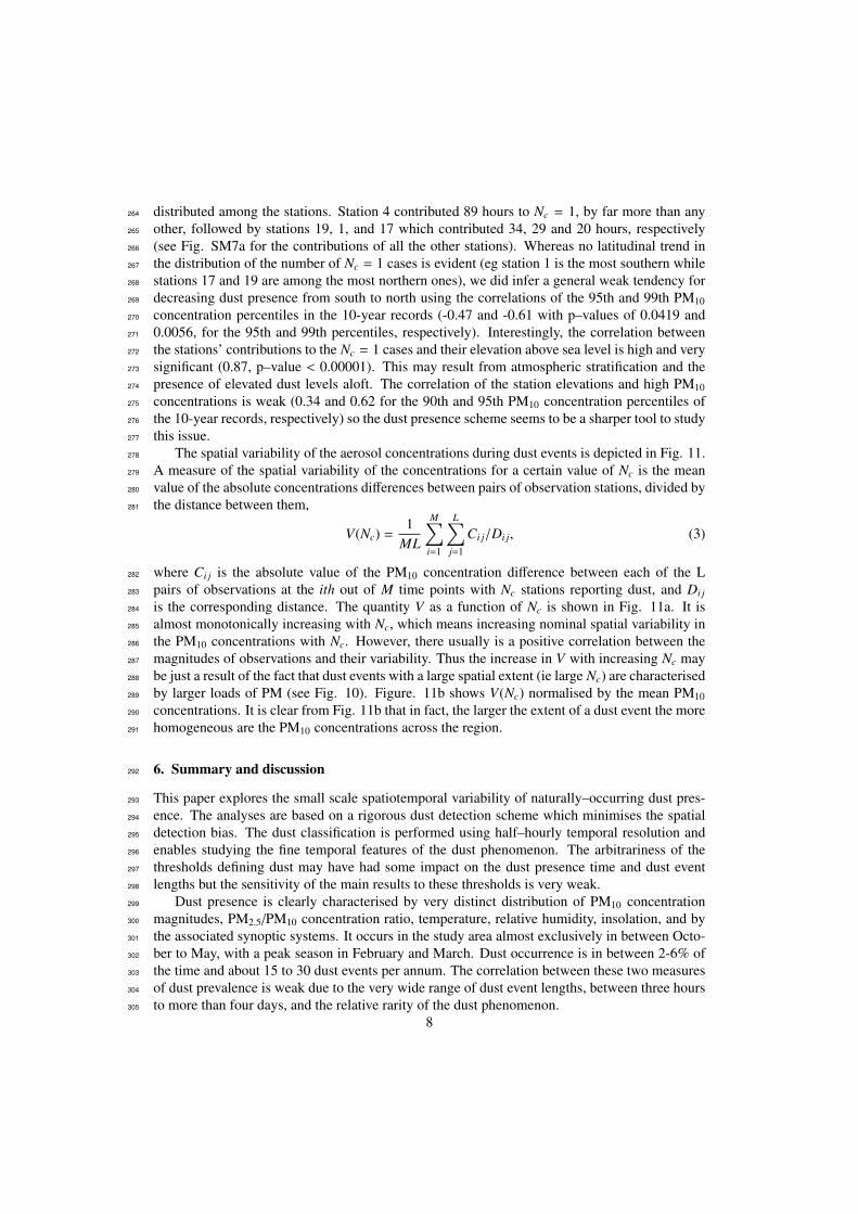
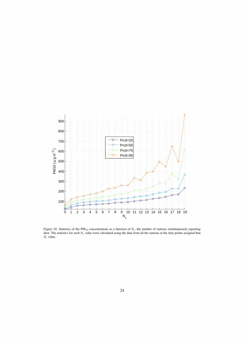
Figure 10 shows the 25th, 50th, 75th and 90th percentiles of the PM10 concentrations as a func-254
tion of Nc. The statistics were calculated based on the PM10 concentrations at all the monitoring255
stations (whether they reported dust or not) for all the time points assigned with a certain Nc256
value. The most important and conspicuous feature of the curves in Fig. 10 is that the PM10257
concentrations increase almost monotonically with Nc. The larger the spatial extent of a dust258
event, the higher are the associated PM10 concentrations. The correlation between Nc and the259
concentration statistics is around 0.9. A second important observation is the very steep increase260
of the PM10 concentration statistics between Nc = 0 and Nc = 1. The doubling of the statistics261
suggests that the Nc = 1 cases are not completely isolated occurrences of high PM10 concen-262
trations. It is interesting to note that the contributions to the cases of Nc = 1 are not equally263
7
distributed among the stations. Station 4 contributed 89 hours to Nc = 1, by far more than any264
other, followed by stations 19, 1, and 17 which contributed 34, 29 and 20 hours, respectively265
(see Fig. SM7a for the contributions of all the other stations). Whereas no latitudinal trend in266
the distribution of the number of Nc = 1 cases is evident (eg station 1 is the most southern while267
stations 17 and 19 are among the most northern ones), we did infer a general weak tendency for268
decreasing dust presence from south to north using the correlations of the 95th and 99th PM10269
concentration percentiles in the 10-year records (-0.47 and -0.61 with p–values of 0.0419 and270
0.0056, for the 95th and 99th percentiles, respectively). Interestingly, the correlation between271
the stations’ contributions to the Nc = 1 cases and their elevation above sea level is high and very272
significant (0.87, p–value < 0.00001). This may result from atmospheric stratification and the273
presence of elevated dust levels aloft. The correlation of the station elevations and high PM10274
concentrations is weak (0.34 and 0.62 for the 90th and 95th PM10 concentration percentiles of275
the 10-year records, respectively) so the dust presence scheme seems to be a sharper tool to study276
this issue.277
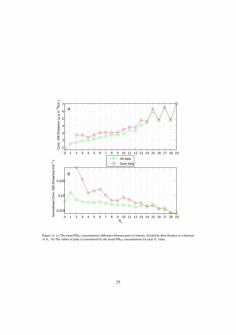
The spatial variability of the aerosol concentrations during dust events is depicted in Fig. 11.278
A measure of the spatial variability of the concentrations for a certain value of Nc is the mean279
value of the absolute concentrations differences between pairs of observation stations, divided by280
the distance between them,281
V(Nc) =1
ML
M∑i=1
L∑j=1
Ci j/Di j, (3)
where Ci j is the absolute value of the PM10 concentration difference between each of the L282
pairs of observations at the ith out of M time points with Nc stations reporting dust, and Di j283
is the corresponding distance. The quantity V as a function of Nc is shown in Fig. 11a. It is284
almost monotonically increasing with Nc, which means increasing nominal spatial variability in285
the PM10 concentrations with Nc. However, there usually is a positive correlation between the286
magnitudes of observations and their variability. Thus the increase in V with increasing Nc may287
be just a result of the fact that dust events with a large spatial extent (ie large Nc) are characterised288
by larger loads of PM (see Fig. 10). Figure. 11b shows V(Nc) normalised by the mean PM10289
concentrations. It is clear from Fig. 11b that in fact, the larger the extent of a dust event the more290
homogeneous are the PM10 concentrations across the region.291
6. Summary and discussion292
This paper explores the small scale spatiotemporal variability of naturally–occurring dust pres-293
ence. The analyses are based on a rigorous dust detection scheme which minimises the spatial294
detection bias. The dust classification is performed using half–hourly temporal resolution and295
enables studying the fine temporal features of the dust phenomenon. The arbitrariness of the296
thresholds defining dust may have had some impact on the dust presence time and dust event297
lengths but the sensitivity of the main results to these thresholds is very weak.298
Dust presence is clearly characterised by very distinct distribution of PM10 concentration299
magnitudes, PM2.5/PM10 concentration ratio, temperature, relative humidity, insolation, and by300
the associated synoptic systems. It occurs in the study area almost exclusively in between Octo-301
ber to May, with a peak season in February and March. Dust occurrence is in between 2-6% of302
the time and about 15 to 30 dust events per annum. The correlation between these two measures303
of dust prevalence is weak due to the very wide range of dust event lengths, between three hours304
to more than four days, and the relative rarity of the dust phenomenon.305
8
Dust covers the whole study area only about 85 hours a year. Most of the time when dust306
is present in the region the coverage is only partial, with the number of dust hours increasing307
as the spatial extent of the dust presence decreases. The events of large spatial extent tend to308
be more intense and more spatially homogeneous in terms of PM concentrations, however, the309
length of dust events is only weakly correlated with their intensity. The SH and WL synoptic310
system groups, both typical winter phenomenon, are the ones most often associated with dust311
events of large spatial extent.312
The majority of dust events (about 56%, see Fig. 6b) are not longer than 12 hours. We thus313
believe that our strategy of employing a high temporal resolution of dust identification enables314
a better specification of the dust phenomenon. The very common use of daily resolution dust315
specification (eg Ganor at el., 2010; Krasnov et al., 2014) might result in misclassification and316
reduced power of the statistical analyses. For example, Ganor et al. (2010) reported elevated317
number of dust days during April occurrences of PT synoptic systems, not known as associated318
with dust. It is very probable that the dust in those cases was actually associated with a Sharav319
Low, a synoptic system which has a sharp peak of prevalence in April but which may be very320
short in duration and thus might not be registered as the synoptic system on its day of occurrence321
(Alpert et al., 2004). Another example is the daily–based dust presence definition of Krasnov et322
al. (2014) which was used by Vodonos et al. (2014) in a study of daily hospitalisations and their323
possible association with exacerbation of chronic obstructive pulmonary disease. Their daily324
mean 71 µgm−3 PM10 concentration threshold to define a day as associated with dust may clearly325
lead to exposure misclassification due to the prevalence of many short dust events. In Fig. 2c326
we depict such an event which straddles the days of 26-05-2005 and 27-05-2005. The mean327
PM10 concentration in both days was above 71 µgm−3. However, the exposure of the population328
was probably minimal as the event took place in between 23:00 and 02:00, and above average329
concentrations were observed only after 21:30 and before 06:00, hours when most people are at330
home and are less exposed to ambient PM.331
Our results reveal some insights that have not been reported thus far and debunk some com-332
mon claims. We have found no clear basis to the assumption made by Krasnov et al. (2014) that333
the majority of natural dust storms take place mainly during the daytime. Figure SM8, produced334
using our high resolution dust detection scheme does not reveal any significant association of335
dust presence and the hour of the day. Any such association is haphazard and vary from station336
to station. We did confirm the claim in the literature of an elevated dust presence in the south337
compared to the north in Israel (eg Ganor and Foner, 2001; Krasnov et al., 2014). This associ-338
ation is weak though and we noted many instances of dust present in northern Israel but not in339
its southern parts. For example, during the study period 2004-2013, during 75 half–hourly time340
points all the southern and central stations (1-12) reported dust while none of the northern ones341
(13-19) did. However, the opposite case (stations 13-19 reporting dust but none of stations 1-12342
does) also occurred during 41 time points. The clear presence of dust only in part of the study343
area and not at all elsewhere is intriguing. Dust is transported by synoptic phenomena with a344
spatial scale of about 1000 km but we notice that intra–regional variations on the tens of km spa-345
tial scale exist. The small scale variability in the dust plumes can be visually seen in Fig. SM6346
in the Supplementary Material. A detailed and interesting glimpse into the conditions during347
various types of dust events is given in Figs. SM9 and SM10 of the Supplementary Material.348
The dust–detection methodology used in this paper enables studying the phenomena depicted349
in Figs. SM8, SM9 and SM10 quantitatively. Additional finding is the frequent prevalence of350
local dust events which can be detected only in a small number of stations. The strong positive351
correlation which we found between the stations’ elevation above sea level and the number of352
9

such occurrences may serve as a hint about the processes by which the dust plumes arrives at the353
surface. As only twice–daily atmospheric stratification data were available, we could not follow354
this lead. We hope that future studies using higher resolution stratification data (eg Uzan and355
Alpert, 2012) will arrive at deeper understanding.356
The Middle East and North Africa region is a large source of dust and it is also one of357
the most affected by dust storms. Much work has been carried out to study the issue of dust358
from the western Maghreb (eg Ozer et al., 2006) through the Arabian peninsula (Maghrabi et359
al., 2011) to the Persian Gulf (eg Hamidi et al., 2013). In most cases the studies concentrated360
on large dust events and the synoptic conditions that bring them about. Our work contributes361
to the understanding of the smaller scale variability in time and space and we hope that our362
methodology will be used to future studies of dust in the region.363
7. Acknowledgments364
The research was supported by the Technion Centre of Excellence in Exposure Science and365
Environmental Health (TCEEH). P.A. would like to acknowledge the support of the Helmholtz366
DESERVE project.367
10
8. References368
Asaf, D., Pedersen, D., Peleg, M., Matveev, V., Luria, M., 2008. Evaluation of background369
levels of air pollutants over Israel. Atmospheric Environment, 42, 8453-8463.370
Alpert, P., Osetinsky, I., Ziv, B., Shafir, H., 2004. Semi–objective classification for daily synop-371
tic system: application to the eastern Mediterranean climate change. International Journal372
of Climatology 24, 1001-1011.373
Dadvand, P., Basagana, X., Figueras, F., Amoly, E., Tobias, A., de Nazelle, A., Querol, X.,374
Sunyer, J., Nieuwenhuijsen, M.J., 2011. Saharan dust episodes and pregnancy. Journal of375
Environmental Monitoring 13, 3222-3228.376
Escudero, M., Castillo, S., Querol, X., Avila, A., Alarcon, M., Viana, M.M., Alastuey, A.,377
Cuevas, E., Rodrıguez, S., 2005. Wet and dry African dust episodes over Eastern Spain.378
Journal of Geophysical Research 110, doi:10.1029/2004JD004731.379
Escudero, M., Querol, X., Avila, A., Cuevas, E., 2007a. Origin of the exceedances of the380
European daily PM limit value in regional background areas of Spain. Atmo- spheric381
Environment 41, 730744.382
Escudero, M., Querol, X., Pey, J., Alastuey, A., Perez, N., Ferreira, F., Cuevas, E., Rodrıguez,383
S., Alonso, S., 2007b. A methodology for the quantification of the net African dust load in384
air quality monitoring networks. Atmospheric Environment 41, 55165524.385
Evan, A.T., Heidinger, A.K., Pavolonis, M.J., 2006. Development of a new over–water Ad-386
vanced Very High Resolution Radiometer dust detection algorithm. International Journal387
of Remote Sensing 27, 3903-3924.388
Ganor, E., Foner, H.A., 2001. Mineral dust concentrations, deposition fluxes and deposition389
velocities in dust episodes over Israel. Journal of Geophysical Research 106: 1843118437.390
Ganor, E., Stupp, A., Alpert, P., 2009. A method to determine the effect of mineral dust aerosols391
on air quality. Atmospheric Environment 43, 54635468.392
Ganor, E., Osetinsky, I., Stupp, A., Alpert, P., 2010. Increasing trend of African dust, over393
49 years, in the eastern Mediterranean. Journal of Geophysical Research 115, D07201,394
doi:10.1029/2009JD012500.395
Goudie, A.S., Middleton, N.J., 2006. Desert dust in the global system. Springer Verlag, Hei-396
delberg: 280pp.397
Goudie, A.S, 2014. Desert dust and human health disorders. Environment International 63,398
101-113.399
Hamidi, M., Kavianpour, M.R., Shao, Y., 2013. Synoptic Analysis of Dust Storms in the Middle400
East. Asia–Pacific Journal of Atmospheric Sciences 49, 279-286.401
Hastie, Tibshirani, R.,Friedman, J., 2009. The Elements of Statistical Learning: Data mining,402
Inference, and Prediction. Springer, New York. 745 pp.403
11
Israelevich, P., Ganor, E., Alpert, P., Kishcha, P., Stupp, A., 2012. Predominant transport paths404
of Saharan dust over the Mediterranean Sea to Europe. Journal of Geophysical Reaserch405
117, D02205, doi:10.1029/2011JD016482.406
Jimenez-Guerrero, P., Perez, C., Jorba, O., Baldasano, J., 2008. Contribution of Saharan dust in407
an integrated air quality system and its on–line assessment. Geophysical Research Letters408
35, L03814.409
Karanasiou, A., Moreno, N., Moreno, T., Viana, M., de Leeuw, F., Querol, X., 2012. Health410
effects from Sahara dust episodes in Europe: literature review and research gaps. Environ-411
ment International 47, 10714.412
Kocak, M., Mihalopoulos, N., Kubilay, N., 2007. Contributions of natural sources to high PM10413
and PM2.5 events in the eastern Mediterranean. Atmospheric Environment 41, 38063818.414
Krasnov., H., Katra, I., Koutrakis, P., Friger, M.D., 2014. Contribution of dust storms to PM10415
levels in an urban arid environment. Journal of the Air & Waste Manahement 64, 89-94.416
Liao, T.W., 2005. Clustering of time series data–a survey. Pattern recognition 38, 1857-1874.417
Maghrabi, A., Alharbi, B., Tapper, N., 2011. Impact of the March 2009 dust event in Saudi Ara-418
bia on aerosol optical properties, meteorological parameters, sky temperature and emissiv-419
ity. Atmospheric Environment, 45, 21642173.420
Mallone, S., Stafoggia, M., Faustini, A., Gobbi, G.P., Matcom, A., Forastiere, F., 2011. Saha-421
ran dust and associations between particulate matter and daily mortality in Rome, Italy.422
Environmental Health Perspectives 119, 1409-1414.423
Matlab 8.1.0.604 (R2013a), 2013. The MathWorks Inc., Natick, Massachusetts.424
Mitsakou, C., Kallos, G., Papantoniou, N., Spyrou, C., Solomos, S., Astitha, M., Housiadas, C.,425
2008. Saharan dust levels in Greece and received inhalation doses. Atmospheric Chem-426
istry and Physics 8, 71817192.427
Ozer, P., Laghdaf, M.B.O.M., Lemine, S.O.M., Gassani, J., 2006. Estimation of air quality428
degradation due to Saharan dust at Nouakchott, Mauritania, from horizontal visibility data.429
Water, Air, and Soil Pollution 178:79-87.430
Pey, J., Querol, X., Alastuey, A., Forastiere, F., Stafoggia, M, 2013. African dust outbreaks431
over the Mediterranean Basin during 20012011: PM10 concentrations, phenomenology432
and trends, and its relation with synoptic and mesoscale meteorology Atmospheric Chem-433
istry and Physics 13, 1395-1410.434
Prospero, J.M., Ginoux, P., Torres, O., Nicholson, S.E. Gill, T.E, 2002. Environmental char-435
acterization of global sources of atmospheric soil dust identified with the nimbus 7 total436
ozone mapping spectrometer (TOMS) absorbing aerosol product. Reviews of Geophysics437
40, 2-31.438
Querol, X., Pey, J., Pandolfi, M., Alastuey, A., Cusack, M., Perez, N., Moreno, T., Viana, M.,439
Mihalopoulos, N., Kallos, G., Kleanthous, S., 2009. African dust contributions to mean440
ambient PM10 mass–levels across the Mediterranean Basin. Atmospheric Environment 43,441
4266-77.442
12
Rodrıguez, S., Querol, X., Alastuey, A., Plana, F., 2002. Sources and processes affecting levels443
and composition of atmospheric aerosol in the Western Mediterranean. Journal of Geo-444
physical Research 107, (D24), 4777.445
Uzan, L., Alpert, P., 2012. The coastal boundary layer and air pollution–a high temporal reso-446
lution analysis in the East Mediterranean coast. The open Atmospheric Sciences Journal447
6, 9-18.448
Viana, M., P. Salvador, B. Artinano, X. Querol, A. Alastuey, J. Pey, A.J. Latz, M. Cabanas, T.449
Moreno, S.G. Dos Santos, M.D. Herce, P.D. Hernandez, D.R. Garcia, and R. Fernandez-450
Patier. 2010. Assessing the performance of methods to detect and quantify African451
dust in airborne particulates. Environmental Science and Technolongy, 44, 88148820.452
doi:10.1021/es1022625453
Vodonos, A., Friger, M., Katra, I., Avnon, L., Krasnov, H., Koutrakis, P., Schwartz, J., Lior,454
O., Novack, V., 2014. The impact of desert dust exposures on hospitalizations due to455
exacerbation of chronic obstructive pulmonary disease. Air Quality, Atmosphere & Health456
7, 433-439.457
Zhang, P., Lu, N., Hu, X., Dong, C., 2006. Identification and physical retrieval of dust storm458
using three MODIS thermal IR channels. Global and Planetary Change 52, 197-206.459
13
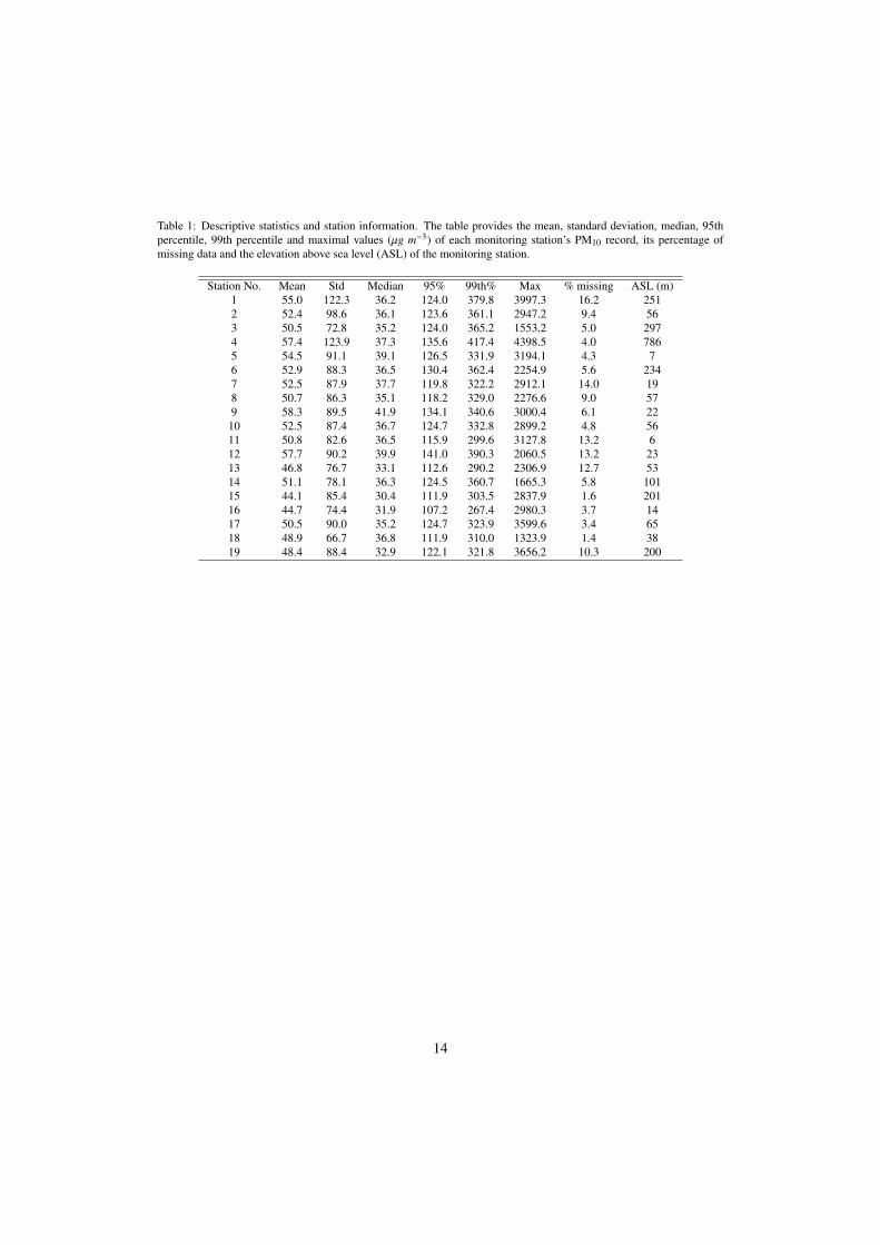
Table 1: Descriptive statistics and station information. The table provides the mean, standard deviation, median, 95thpercentile, 99th percentile and maximal values (µg m−3) of each monitoring station’s PM10 record, its percentage ofmissing data and the elevation above sea level (ASL) of the monitoring station.
Station No. Mean Std Median 95% 99th% Max % missing ASL (m)1 55.0 122.3 36.2 124.0 379.8 3997.3 16.2 2512 52.4 98.6 36.1 123.6 361.1 2947.2 9.4 563 50.5 72.8 35.2 124.0 365.2 1553.2 5.0 2974 57.4 123.9 37.3 135.6 417.4 4398.5 4.0 7865 54.5 91.1 39.1 126.5 331.9 3194.1 4.3 76 52.9 88.3 36.5 130.4 362.4 2254.9 5.6 2347 52.5 87.9 37.7 119.8 322.2 2912.1 14.0 198 50.7 86.3 35.1 118.2 329.0 2276.6 9.0 579 58.3 89.5 41.9 134.1 340.6 3000.4 6.1 22
10 52.5 87.4 36.7 124.7 332.8 2899.2 4.8 5611 50.8 82.6 36.5 115.9 299.6 3127.8 13.2 612 57.7 90.2 39.9 141.0 390.3 2060.5 13.2 2313 46.8 76.7 33.1 112.6 290.2 2306.9 12.7 5314 51.1 78.1 36.3 124.5 360.7 1665.3 5.8 10115 44.1 85.4 30.4 111.9 303.5 2837.9 1.6 20116 44.7 74.4 31.9 107.2 267.4 2980.3 3.7 1417 50.5 90.0 35.2 124.7 323.9 3599.6 3.4 6518 48.9 66.7 36.8 111.9 310.0 1323.9 1.4 3819 48.4 88.4 32.9 122.1 321.8 3656.2 10.3 200
14
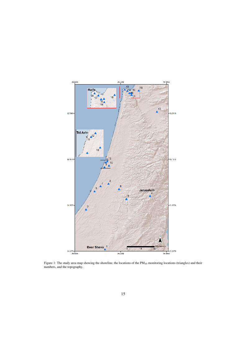
Figure 1: The study area map showing the shoreline, the locations of the PM10 monitoring locations (triangles) and theirnumbers, and the topography.
15
3 6 9 12 15 18 21 24
80
100
120
140
160
180
200
Hour
Con
c. (
µ g
m−
3 )
a
3 6 9 12 15 18 21 24
50
100
150
200
Hour
Con
c. (
µ g
m−
3 )
b
3 6 9 12 15 18 21 24 3 6 9 12 15 18 21 24
50
100
150
200
250
300
350
Hour
Con
c. (
µ g
m−
3 )
c
6 12 18 24 6 12 18 24 6 12 18 24
100
200
300
400
500
Hour
Con
c. (
µ g
m−
3 )
d
3 6 9 12 15 18 21 24
200
400
600
800
1000
Hour
Con
c. (
µ g
m−
3 )
e
6 12 18 24 6 12 18 24 6 12 18 24 6 12 18 24 6 12 18 240
500
1000
1500
2000
2500
3000
Hour
Con
c. (
µ g
m−
3 )
f
Figure 2: Examples of PM10 concentration time series on days when dust events were detected in station 9. The timepoints flagged as dust–related are highlighted in green. The solid and dashed lines mark the values used in the criteriadefining the cluster centres as dust event (see section 4.1 for more details). (a) Event from 09:00 to 21:00 on 04-01-2004(12.0 hours), synoptic system group: Winter Low. (b) Event from 13:00 to 20:00 on 02-02-2006 (7.0 hours), synopticsystem group: Sharav Low. (c) Event from 23:00 on 26-05-2005 to 02:00 on 27-05-2006 (3.5 hours), synoptic systemgroup: unknown, the very short event’s duration did not include the 12:00 UTC hour, the time for which the synopticsystems were classified. (d) Event from 12:00 on 21-10-2011 to 08:00 on 23-10-2011 (45 hours), synoptic system group:Red Sea Trough. (e) Event from 15:00 to 19:00 on 31-03-2005 (5 hours), synoptic system group: Sharav Low. (f) Eventfrom 16:00 on 25-02-2006 to 21:00 on 01-03-2006 (101.5 hours), synoptic system group: changing from Winter Low(26-02 and 27-02) to Siberian High (28-02) and to Winter Low again (01-03).
16
0 20 40 60 80 100 120 1400
2000
4000
6000
8000
10000
12000
Occ
urre
nce
a
0 200 400 600 800 1000 1200 1400 16000
500
1000
1500
2000
PM10 Conc.( µ g m−3 )
Occ
urre
nce
b
Figure 3: The empirical probability density distributions of PM10 concentrations in station 9 of (a) the sample of normaltime points and (b) the sample of time points flagged as associated with dust. Values above the 99% percentile of thesamples were not used for the plots for visual purposes.
17
0.1 0.2 0.3 0.4 0.5 0.6 0.7 0.8 0.90
2000
4000
6000
Occ
urre
nce
a
0.1 0.2 0.3 0.4 0.5 0.6 0.7 0.8 0.90
100
200
300
400
500
600
[PM2.5]/[PM10]
Occ
urre
nce
b
Figure 4: The empirical probability density distributions of the PM2.5/PM10 concentration ratio in station 9 of (a) thesample of normal time points and (b) the sample of time points flagged as associated with dust.
18
RST PT HW SH WL SL0
200
400
600
800
1000
Occ
urre
nce
a
RST PT HW SH WL SL0
10
20
30
40
50
Synoptic System Group
Occ
urre
nce
b
Figure 5: The number of 12:00 UTC time points which were classified to each of the synoptic system groups based onthe data from station 9. (a) The sample of normal time points. (b) The sample of time points flagged as associated withdust. The synoptic systems groups are: Red Sea Troughs (RST), Persian Trough (PT), High to the West (HW), SiberianHighs (SH), Winter Lows (WL) and Sharav Low (SL). See details in Alpert et al. (2004).
19
0 4 8 12 16 20 24 28 32 36 40 44 48 52 56 60 64 68 720
10
20
30
40
50
60
70
Event length ( hours )
Occ
urre
nce
a
20 40 60 80 100 120 140 160 180 200 220
20
40
60
80
100
Event number
Eve
nt le
ngth
( ho
urs
) b
Figure 6: Dust events lengths based on the dust flagging scheme using the data from station 9. (a) Histogram of dustevent lengths up to 72 hours. (b) All the dust event lengths sorted by their length.
20
Jan Feb Mar Apr May Jun Jul Aug Sep Oct Nov Dec0
1
2
3
4
No.
of e
vent
s
a
Jan Feb Mar Apr May Jun Jul Aug Sep Oct Nov Dec0
20
40
60
Calendar months
No.
of h
ours
b
Figure 7: The annual cycle of dust presence based on the dust flagging scheme using the data from station 9. (a) Themean number of dust events per calendar month. (b) The mean number of dust-related hours per calendar month.
21
2004 2005 2006 2007 2008 2009 2010 2011 2012 2013
16
20
24
28
Years
No.
of e
vent
s
2004 2005 2006 2007 2008 2009 2010 2011 2012 20132
4
6
Per
cent
of d
ust−
rela
ted
time
Figure 8: The inter-annual variability of the dust phenomenon, depicted by the number of dust events and the percentageof dust–related time points.
22
1 2 3 4 5 6 7 8 9 10 11 12 13 14 15 16 17 18 190
50
100
150
200
250
Nc
Hou
rs
Figure 9: The empirical probability distribution of the mean annual number of PM10 stations simultaneously reportingdust during the study period.
23
0 1 2 3 4 5 6 7 8 9 10 11 12 13 14 15 16 17 18 19
100
200
300
400
500
600
700
800
900
Nc
PM
10 (
µ g
m−
3 )
Prctl=25Prctl=50
Prctl=75Prctl=90
Figure 10: Statistics of the PM10 concentrations as a function of Nc, the number of stations simultaneously reportingdust. The statistics for each Nc value were calculated using the data from all the stations at the time points assigned thatNc value.
24
0 1 2 3 4 5 6 7 8 9 10 11 12 13 14 15 16 17 18 19
1
2
3
4
5
6
7
Con
c. D
iff./D
ista
nce
( µ g
m−
3 /Km
)
a
All data
Dust data
0 1 2 3 4 5 6 7 8 9 10 11 12 13 14 15 16 17 18 19
0.015
0.02
0.025
Nor
mal
ised
Con
c. D
iff./D
ista
nce(
Km
−1 )
Nc
b
Figure 11: (a) The mean PM10 concentrations difference between pairs of stations, divided by their distance as a functionof Nc. (b) The values of plate (a) normalised by the mean PM10 concentrations for each Nc value.
25