Chapter 6

Economic Impacts of Enhanced ASEAN-India Connectivity: Simulation Results from IDE/ERIA-GSM Satoru Kumagai Institute of Developing Economies, Japan External Trade Organization (IDE-JETRO) Ikumo Isono Economic Research Institute for ASEAN and East Asia (ERIA) December 2011 This chapter should be cited as Kumagai, S. and I. Isono (2011), ‘Economic Impacts of Enhanced ASEAN-India Connectivity: Simulation Results from IDE/ERIA-GSN’ in Kimura, F. and S. Umezaki (eds.), ASEAN-India Connectivity: The Comprehensive Asia Development Plan, Phase II, ERIA Research Project Report 2010-7, Jakarta: ERIA, pp.243-307.

243

CHAPTER 6.

ECONOMIC IMPACTS OF ENHANCED ASEAN-INDIA CONNECTIVITY:

SIMULATION RESULTS FROM IDE/ERIA-GSM

SATORU KUMAGAI

IKUMO ISONO

Abstract

We have been developing the IDE/ERIA Geographical Simulation Model

(IDE/ERIA-GSM) since 2007, and now the model has reached the 5th version (Kumagai et

al. 2012). By using IDE/ERIA-GSM, we conduct several simulations to estimate the

economic impacts of various trade and transport measures (TTFMs) concerning

ASEAN-India Connectivity1

1 General explanation of IDE/ERIA-GSM 5, including model, parameters and data, is provided in Appendix.

244

1. INTRODUCTION

Infrastructure development as well as logistics enhancement is one of the most

important key drivers for economic development. We still have huge gaps both in

economic development and in logistics infrastructures in East Asia. To pursue higher

economic development and to narrow the economic gaps, it goes without saying that we

need much effort in the region.

This chapter provides some policy implications for better ASEAN-India

Connectivity by using IDE/ERIA Geographical Simulation Model (IDE/ERIA-GSM).

IDE/ERIA-GSM is a simulation model based on spatial economics, also known as new

economic geography. It can be used as a tool for policy makers to judge about what

kinds of trade and transport measures (TTFMs) are needed, how to prioritize them and

how to mingle them. The model has an original economic model with general

equilibrium setting, original simulation programs running on JAVA, huge dataset consists

of 1,715 regions, 4,266 nodes and 7,044 routes, and several parameters obtained by

econometric techniques. It covers 18 countries/economies in Asia in addition to two

economies of the U.S. and European Union (EU); Bangladesh, Brunei Darussalam,

Cambodia, China, Hong Kong, India, Indonesia, Japan, Korea, Lao PDR, Macao,

Myanmar, Malaysia, the Philippines, Singapore, Chinese Taipei, Thailand, and Vietnam.

The model makes it possible to estimate the economic impacts of various TTFMs, e.g.

economic impacts on each Indian state of a road improvement in Myanmar, and is well

accorded with the cluster approach and economic corridor approach.

This chapter is structured as follows: Section 2 constructs the baseline scenario and

explains its assumptions. Section 3 gives additional alternative scenarios concerning

ASEAN-India connectivity. Section 4 concludes with some policy implications.

2. INFRASTRUCTURE DEVELOPMENT IN INDIA AND THE BASELINE SCENARIO

In this section, we explain the baseline scenario in this chapter. We have the

baseline scenario, other alternative scenarios and a scenario without any development

245

projects as in Figure 1. We call the last one “no projects” scenario. In all scenarios,

the simulation starts from 2005. In 2010, we have some TTFMs in the baseline and

other alternative scenarios, representing already completed projects by 2010, such as the

Golden Quadrilateral (GQ) of India. Also, we have other TTFMs in 2015 in both

baseline and alternative scenarios, presuming some TTFMs such as the improvements of

North-South and East-West Corridor (NSEW) of India will be implemented by 2015.

On the other hand, in the “no projects” scenario we don’t have any TTFMs after 2005.

We incorporate not only already completed projects but also some on-going projects

in the baseline scenario. It is because our objective is to estimate the net benefit of

additional projects planned in ASEAN-India connectivity. It also helps to identify

which areas these projects contribute for, and which areas we should focused on further.

Figure 1: Difference between Baseline Scenario and other Alternative Scenarios

Source: Authors.

The following macro parameters are maintained across scenarios:

There is no immigration between the region covered in the simulation and the rest of

the world.

The national population of each country is assumed to increase at the rate forecasted

by the United Nations Population Division until year 2030, as specified in Table A16

in Appendix.

2005 

2010 with GQ and

Poipet‐Sisophon highway 

2015 

Baseline Scenario with NSEW of India and 

Yangon‐Mandalay highway   in 2015   

Alternative Scenarios with additional development 

projects in 2015 to the baseline 

2030 Compare the differences 

(15 years after) 

GDP/GRDP 

“No Projects” Scenario Scenario without any development projects in 2010 and 2015 

Economic Impact(% of GDP of baseline in 2030) 

246

2-1. Specification for the Baseline Scenario

In principle, the basic speed of land traffic is set to 38.5 km/h and fixed for all years.

However, because of the better road conditions compared to transport demand for them,

we assume that the speed of highways in Thailand (excluding surrounding area of

Bangkok), between Bukit Kayu Hitam and Singapore via Kuala Lumpur, and between

Sisophon and Bavet is 60km/h and the speed passing through mountainous areas is set

to half of the basic at—19.25 km/h. As for sea traffic, the average speed is set to 29.4

km/h for international-class routes, and at half of that among other routes. For air

traffic, the average speed is set to 800 km/h between the primary airports2 of each

country and at 400 km/h among other routes. As for railway traffic, the average speed

is set at 19.1 km/h.

In the “no projects” scenario and the baseline scenario, we prohibit transit transport

through Myanmar and Bangladesh. Therefore, in this case trade between China and

India is mainly done by ocean routes passing through Malacca Straits, or by air routes.

Also, firms in Thailand and Laos usually use Laem Chabang port to export to India or

EU.

In baseline scenarios as well as other alternative scenarios, we have improved GQ

of India and the road between Poipet and Sisophon in 2010, by raising the speed of

them to 60km/h. Figure 2 shows the economic impacts of GQ on India. Note that

this figure compares two economies in 2030 as follows:

GQ Scenario: An economy where we have improved GQ in 2010 but no other

projects after 2005.

No projects Scenario: The other artificial economy where we hadn’t had any

infrastructure development projects after 2005.

2 In this simulation, we designated the following airports as primary airports: Brunei Intl

Airport,Changi Intl Airport, Hong Kong Intl Airport, Kuala Lumpur Intl Airport, Ninoy Aquino Intl Airport, SoekarnoHatta Intl Airport, Suvarnabhumi Intl Airport, Phnom Penh Intl Airport, Yangon Intl Airport, Wattay Intl Airport, Tansonnhat Intl Airport, Chennai Intl Airport, Noibai Intl Airport

247

Figure 2: Economic Impacts of Golden Quadrilateral (GQ) of India (2030, compared with the “No projects” Scenario without any

Development Projects in 2010 and 2015)3

Note: NA for Jammu and Kashmir due to data availability. Source: IDE/ERIA-GSM 5.

After having the better highway, firms in the model along GQ get the benefit in

selling and buying products in better price, thanks to the lowered transport costs. This

stimulates economic activities and thus raises GRDP of the regions along GQ in 2030.

Moreover, some firms in Middle and North-East India move to regions along GQ to

seek higher profits, and some people also move to the regions to get better incomes.

These behaviors push up the GRDP of the regions along GQ further, while Middle and

North-East India may suffer losing GRDP, even if we weigh the GQ scenario against the

scenario with no infrastructure developments.

In the baseline scenario, we also assume that we will have better highways along

with NSEW in India and highway between Yangon and Mandalay in 2015, because

these projects are on-going now and no doubt we will complete these projects by 2015.

Figure 3 depicts the economic impacts of NSEW of India, comparing the “No Projects”

3 We couldn’t obtain the results for Jammu and Kashmir because the geo-mapping data based on the Global Administrative Unit Layers(GAUL) dataset by FAO doesn’t meet our socio-economic dataset for the region.

248

scenario.

Thanks to the development of NSEW, economic activities along these economic

corridors are revitalized, leading to the higher GRDP. Some of regions along GQ may

suffer slightly compared with GQ scenario, because relative attractiveness of these

regions to firms and people will slightly decline. However, Figure 3 tells us that these

regions still have obvious positive impacts compared to the scenario without any

development projects.

Figure 3: Economic Impacts of GQ and NSEW of India (2030, compared with the “No projects” Scenario without any Development Projects in 2010 and 2015)

Source: IDE/ERIA-GSM 5.

2-2. Simulations on Basic Infrastructure Developments in India and Myanmar up to 2015 compared with the Baseline Scenario

In the last subsection, two simulations were conducted comparing the economies in

2030 between GQ development in 2010 with no developments, and between GQ in

2010 and NSEW of India in 2015 with no developments.

To understand the baseline scenario more clearly, let us illustrate the simulation

results of no projects scenario, GQ scenario, GQ+NSEW of India scenario, comparing

249

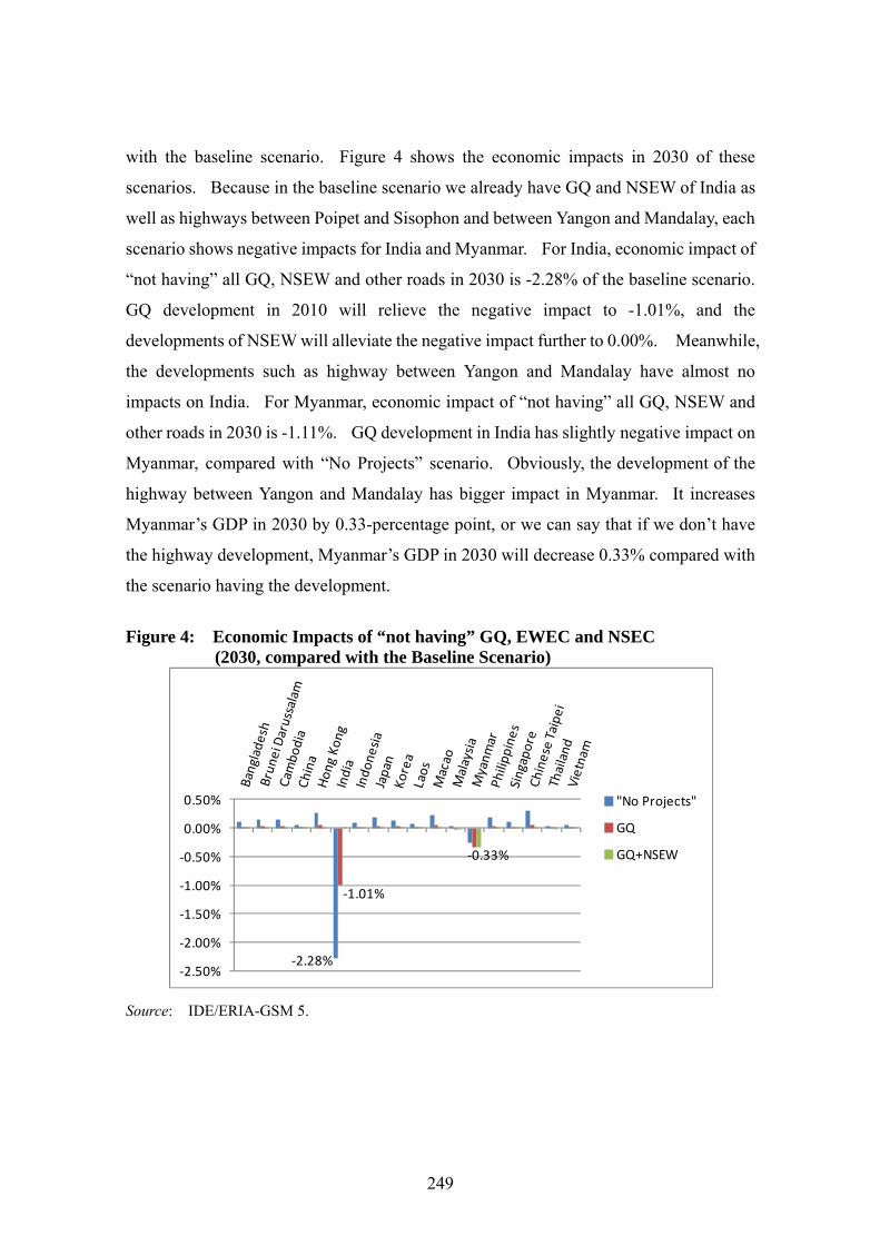
with the baseline scenario. Figure 4 shows the economic impacts in 2030 of these

scenarios. Because in the baseline scenario we already have GQ and NSEW of India as

well as highways between Poipet and Sisophon and between Yangon and Mandalay, each

scenario shows negative impacts for India and Myanmar. For India, economic impact of

“not having” all GQ, NSEW and other roads in 2030 is -2.28% of the baseline scenario.

GQ development in 2010 will relieve the negative impact to -1.01%, and the

developments of NSEW will alleviate the negative impact further to 0.00%. Meanwhile,

the developments such as highway between Yangon and Mandalay have almost no

impacts on India. For Myanmar, economic impact of “not having” all GQ, NSEW and

other roads in 2030 is -1.11%. GQ development in India has slightly negative impact on

Myanmar, compared with “No Projects” scenario. Obviously, the development of the

highway between Yangon and Mandalay has bigger impact in Myanmar. It increases

Myanmar’s GDP in 2030 by 0.33-percentage point, or we can say that if we don’t have

the highway development, Myanmar’s GDP in 2030 will decrease 0.33% compared with

the scenario having the development.

Figure 4: Economic Impacts of “not having” GQ, EWEC and NSEC (2030, compared with the Baseline Scenario)

Source: IDE/ERIA-GSM 5.

‐2.28%

‐1.01%

‐0.33%

‐2.50%

‐2.00%

‐1.50%

‐1.00%

‐0.50%

0.00%

0.50% "No Projects"

GQ

GQ+NSEW

250

3. ADDITIONAL ALTERNATIVE SCENARIOS

This section introduces additional alternative scenarios and compares with the

baseline scenario. We have several scenarios on ASEAN-India Connectivity as

follows:

a. Comparison between Dawei deep seaport and Pak Bara deep seaport.

b. Mekong-India Economic Corridor (MIEC).

c. Kyaukphyu deep seaport.

d. Trilateral Highway (TH).

e. “South Route” connecting Mae Sot to Siliguri with better highways.

f. “South Route+x”, adding the routes between Dhaka and Kolkata and between

Kanchanaburi and Thaton to South Route.

g. “North Route” connecting Mae Sai to Moreh (or Silchar) with better highways.

h. “North Route+x”, adding the routes between Silchar to Dhaka and between

Guwahati to Dhaka.

i. All Developments.

j. All Developments with reduction of Policy and Cultural Barriers (PCBs).

3-1. Two Deep Seaport Projects and MIEC

We consider two deep seaport projects in Andaman seaside, that is, Dawei deep

seaport project in Myanmar and Pak Bara deep seaport project in Thailand.

We set five different scenarios as follows:

Dawei (No Transit)

Development of Dawei Port and highway between Kanchanaburi and Dawei in

2015.

Customs facilitation at the Kanchanaburi-Dawei border.

Connecting Dawei to Kolkata, Chennai, and Rotterdam by international equivalent

sea routes.

Fixed PCBs.

251

Dawei

In addition to the Dawei (No Transit) scenario, the transit transport through

Myanmar only when firms use both Dawei port and the Kanchanaburi-Dawei

border to be allowed.

Special customs facilitation that products of Thailand, Laos, Cambodia and other

countries to be exported to India or EU can go through Kanchanaburi to Dawei very

smoothly, at 15 minutes and free-of-charge, and vice versa.

Pak Bara

Development of Pak Bara Port and highway connecting to national highway.

Connecting Pak Bara to Kolkata, Chennai, and Rotterdam by international

equivalent sea routes.

Fixed PCBs.

Dawei+Pak Bara

Development of both Dawei and Pak Bara, including all related measures

mentioned above.

Fixed PCBs.

Figure 5 shows the economic impacts of the five different scenarios in 2030,

compared with the baseline scenario. In Dawei (No Transit) scenario, only Myanmar

has a positive impact while the others have almost no impacts. It this sense, allowing

the transit transport in Myanmar is critical for other countries, especially for Thailand.

Dawei project has larger impact than Pak Bara project for Thailand even though Pak

Bara is a project in Thailand and Dawei is in Myanmar. Furthermore, there is almost

no additional impact when we compare Dawei project only and both Dawei and Pak

Bara projects.

252

Figure 5: Economic Impacts of Four Different Scenarios (2030, compared with the baseline scenario)

Source: IDE/ERIA-GSM 5.

In addition to the Dawei scenario, we consider the enhanced connectivity along

MIEC as follows:

MIEC

Infrastructure Development of the Bridge at Neak Loueng, new highway between

Kanchanaburi and Dawei, and Dawei Port in 2015, leading to the speed-up to

60km/h along the road.

Customs facilitation, meaning that time and costs at the 3 border points at

Kanchanaburi-Dawei, Poipet-Sisophon and Bavet-Moc Bai are halved.

Special customs facilitation that products of Thailand, Laos, Cambodia and other

countries to be exported to India or EU can go through Kanchanaburi to Dawei very

smoothly, at 15 minutes and free-of-charge, and vice versa.

Connecting Dawei and Chennai, and Dawei and Rotterdam by international

equivalent sea routes.

Reducing PCBs 2% per year in Vietnam, Cambodia, Thailand, Myanmar and India.

Figure 6 presents the economic impact of MIEC. Taninthayi, where the capital

city is Dawei, has the largest impact. Enhancement of physical and institutional

connectivity brings large economic impacts on related countries.

‐0.10%

0.00%

0.10%

0.20%

0.30%

0.40%

0.50%

0.60%

Dawei(NT)

Dawei

PakBara

DaweiPakBara

253

Figure 6: Economic Impacts of MIEC with Soft Infrastructure Improvement

(2030, compared with baseline scenario)

Source: IDE/ERIA-GSM 5.

3-2. Kyaukphyu Deep Seaport

In Kyaukphyu deep seaport project, we assume as follows:

Development of Kyaukphyu Port and highway between Muse and Kyaukphyu in

2015.

Customs facilitation at the Muse-Ruili border.

Connecting Kyaukphyu to Kolkata, Chennai, and Rotterdam by international

equivalent sea routes.

The transit transport through Mynmar only when firms use both Kyaukphyu port

and the Muse-Ruili border to be allowed.

Special customs facilitation that products of China and other countries to be exported

to India or EU can go through Ruili to Muse very smoothly, at 15 minutes and

free-of-charge, and vice versa.

254

Reducing PCBs 2% per year in China, Myanmar and India.

Figure 7 illustrates the economic impact of Kyaukphyu project. Myanmar and

China will have large positive impacts. Particularly, the transit transport using

Kyaukphyu port and the Muse-Ruili border makes it possible for the firms and people in

Western China to trade with India and EU without passing Malacca Straits.

Figure 7: Economic Impacts of Kyaukphyu Deep Seaport with Soft Infrastructure Improvement (2030, compared with baseline scenario)

Source: IDE/ERIA-GSM 5.

3-3. Trilateral Highway

In Trilateral Highway project, we set two scenarios as follows:

Trilateral Highway (TH)

Development of New highway running.

Silchar-Moreh/Tamu-Pale-Bagan-Theinzayat-Mawlamyine-Kawkareik-Myawaddy/

255

Mae Sot.

Customs facilitation at the Moreh/Tamu and Myawaddy/Mae Sot borders.

Allowing the transit transport in Myanmar only when firms use the road.

Fixed PCBs.

Trilateral Highway (TH-alternative)

Development of highways between the Moreh/Tamu border and Mandalay and

between Payagyi and Myawaddy/Mae Sot via Hpa An.

Customs facilitation at the Moreh/Tamu and Myawaddy/Mae Sot borders.

Allowing the transit transport in Myanmar only when firms use the road.

Fixed PCBs.

TH scenario describes the new highway project proposed by Myanmar Government.

Having an additional bypass through Myanmar in addition to the Mandalay-Yangon

Highway will make extra positive impacts. TH-alt means highway project along with

Asian Highway No. 1. Connecting the border areas and large cities such as Mandalay,

Bago and Yangon will make additional benefit.

Figure 8 shows the comparison of two Trilateral Highway scenarios. In this case,

TH-alt has larger impact which means having better connection between border areas

and large cities will benefit more. Figure 9 compares the impacts on each Myanmar

state/region. Chin, Kayin and Mon states will get larger positive impacts.

256

Figure 8: Economic Impacts of Trilateral Highway (2030, compared with baseline scenario)

TH TH-alt

Source: IDE/ERIA-GSM 5.

Figure 9: Economic Impacts of Trilateral Highway on Myanmar (2030, compared with baseline scenario)

Source: IDE/ERIA-GSM 5.

3-4. Kaladan River Project

The scenario for Kaladan River project is set as follows:

Connecting Kolkata port to Sittwe port.

Develop new Inland waterway between Sittwe and Paletwa.

‐2.0%

0.0%

2.0%

4.0%

6.0%

8.0%

10.0%

12.0%

14.0%

16.0%

18.0%

20.0%

TH

TH‐alt

257

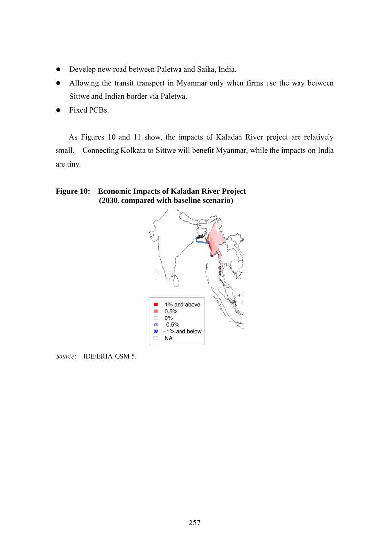
Develop new road between Paletwa and Saiha, India.

Allowing the transit transport in Myanmar only when firms use the way between

Sittwe and Indian border via Paletwa.

Fixed PCBs.

As Figures 10 and 11 show, the impacts of Kaladan River project are relatively

small. Connecting Kolkata to Sittwe will benefit Myanmar, while the impacts on India

are tiny.

Figure 10: Economic Impacts of Kaladan River Project (2030, compared with baseline scenario)

Source: IDE/ERIA-GSM 5.

258

Figure 11: Economic Impacts of Kaladan River Project on India (2030, compared with baseline scenario)

Source: IDE/ERIA-GSM 5.

3-5. “South” and “North” Routes

In the South and North Route scenarios, we set four scenarios as follows:

South Route Scenario

Better highway between Mae Sot and Siliguri, via Thaton, Bago, Pyay, Chittagong,

and Dhaka leading to the speed-up to 60km/h along the road.

Customs facilitation at the borders along the highway.

Allowing the transit transport along the road.

Fixed PCBs.

South Route+x Scenario

Additional better highways between Dhaka and Kolkata and between Kanchanaburi

and Thaton to South Route Scenario, to connect the large cities.

Allowing the transit transport along the road.

Fixed PCBs.

0.043%

0.033%

‐0.005%0.000%0.005%0.010%0.015%0.020%0.025%0.030%0.035%0.040%0.045%0.050%

259

North Route Scenario

Better highway between Mae Sai and Silchar, via Mandalay leading to the speed-up

to 60km/h along the road.

Customs facilitation at the borders along the highway.

Allowing the transit transport along the road.

Fixed PCBs.

North Route+x Scenario

Additional better highways between Silchar to Dhaka and between Guwahati to

Dhaka to North Route Scenario.

Allowing the transit transport along the road.

Fixed PCBs.

Figure 12 depicts the economic impacts of South Route+x Scenario. Figure 13

shows the impacts of North Route+x Scenario.

Figure 12: Economic Impacts of South Route+x Scenario (2030, compared with the baseline scenario)

Source: IDE/ERIA-GSM 5.

260

Figure 13: Economic Impacts of North Route+x Scenario (2030, compared with the baseline scenario)

Source: IDE/ERIA-GSM 5.

Figures 14 and 15 compare the impacts of the four different scenarios on each state

in India. Figure 14 uses the percentage of each state’s GRDP as of 2030 in the

baseline scenario, explaining importance of impacts on each state. Figure 15, on the

other hand, uses an index where the total GDP of India in 2030 in the baseline scenario

is 10,000, denoting importance of impacts on the whole country, or absolute value. We

find North-East India will benefit by North and North+x scenarios. Manipur, Mizoram

and Tripura will have negative impacts by South route, because the route doesn’t

connect these states.

261

Figure 14: Economic Impacts of South and North Route Scenarios on India (percentages, 2030, compared with baseline scenario)

Source: IDE/ERIA-GSM 5.

Figure15: Economic Impacts of South and North Route Scenarios on India (indices, 2030, compared with baseline scenario)

Note: Total GDP of India (2030, the baseline scenario)=10,000 Source: IDE/ERIA-GSM 5.

‐2.00%

0.00%

2.00%

4.00%

6.00%

8.00%

10.00%

12.00%

14.00%

16.00%

18.00%

20.00%

South South+x North North+x

‐4

‐3

‐2

‐1

0

1

2

3

4

5

6

South South+x North North+x

262

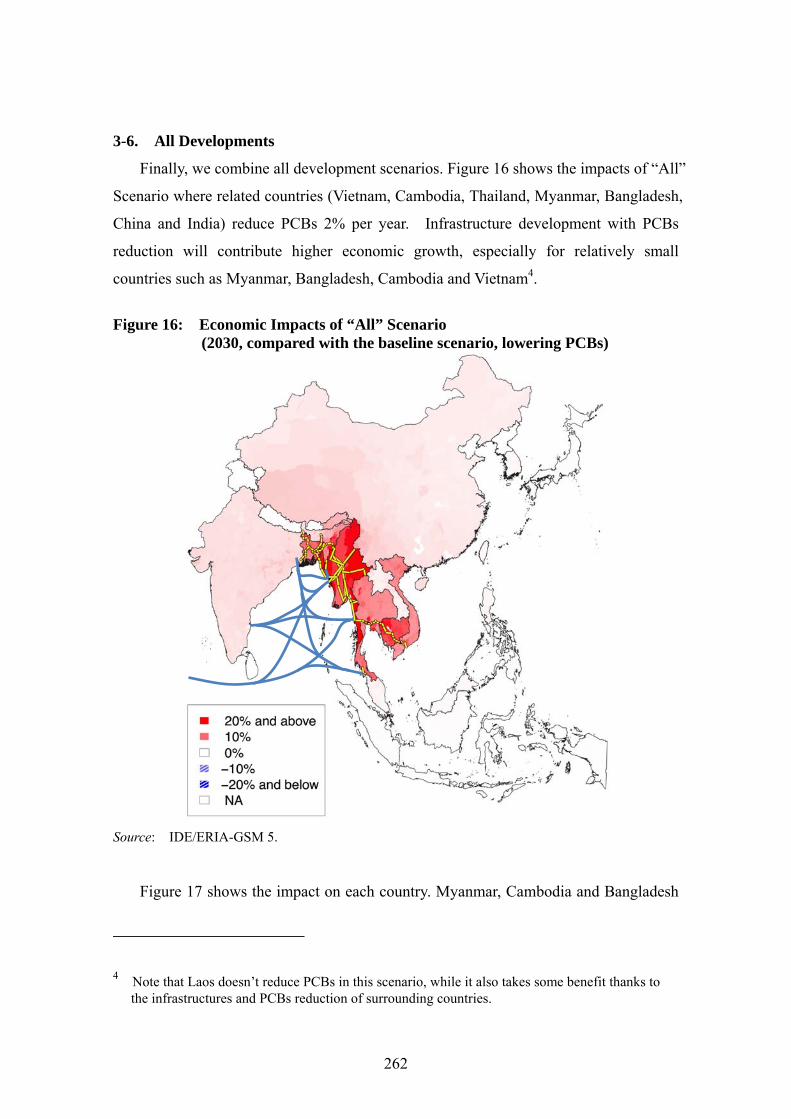
3-6. All Developments

Finally, we combine all development scenarios. Figure 16 shows the impacts of “All”

Scenario where related countries (Vietnam, Cambodia, Thailand, Myanmar, Bangladesh,

China and India) reduce PCBs 2% per year. Infrastructure development with PCBs

reduction will contribute higher economic growth, especially for relatively small

countries such as Myanmar, Bangladesh, Cambodia and Vietnam4.

Figure 16: Economic Impacts of “All” Scenario (2030, compared with the baseline scenario, lowering PCBs)

Source: IDE/ERIA-GSM 5.

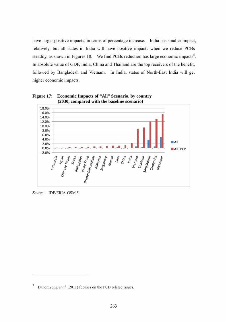
Figure 17 shows the impact on each country. Myanmar, Cambodia and Bangladesh

4 Note that Laos doesn’t reduce PCBs in this scenario, while it also takes some benefit thanks to the infrastructures and PCBs reduction of surrounding countries.

263

have larger positive impacts, in terms of percentage increase. India has smaller impact,

relatively, but all states in India will have positive impacts when we reduce PCBs

steadily, as shown in Figures 18. We find PCBs reduction has large economic impacts5.

In absolute value of GDP, India, China and Thailand are the top receivers of the benefit,

followed by Bangladesh and Vietnam. In India, states of North-East India will get

higher economic impacts.

Figure 17: Economic Impacts of “All” Scenario, by country (2030, compared with the baseline scenario)

Source: IDE/ERIA-GSM 5.

5 Banomyong et al. (2011) focuses on the PCB related issues.

‐2.0%0.0%2.0%4.0%6.0%8.0%

10.0%12.0%14.0%16.0%18.0%

All

All+PCB

264

Figure 18: Economic Impacts of “All” Scenarios on India (percentages, 2030,compared with baseline scenario)

Source: IDE/ERIA-GSM 5.

4. CONCLUSIONS AND POLICY IMPLICATIONS

Better connectivity between ASEAN and India will benefit ASEAN newcomers and

Bangladesh in terms of percentages of each country, and mainly benefit India and

Thailand in terms of absolute value of GDP. We conclude with some findings and

policy implications from the simulation results.

For India, the developments of GQ and NSEW have larger positive impacts than the

additional alternative scenarios, meaning that connecting the domestic market is

crucial.

However, some areas in Middle India may be left behind from the economic

development, as shown in Figure 3. GQ and NSEW are not enough for the areas,

even though these projects have large positive impacts on national GDP.

India will have greater positive impacts by reducing PCBs, together with several

projects discussed above. It is implying that soft infrastructure development is a key

to maximize the benefit of better connectivity.

For Myanmar, both the development of highways and PCBs reduction are essential.

‐5.0%

0.0%

5.0%

10.0%

15.0%

20.0%

25.0%

All All+PCB

265

To reduce PCBs, we need several measures, such as shortening the time for

procedures before shipping, providing information in appropriate languages,

enhancing the capacity of medium-sized firms, and establishing more reliable

dispute settlement.

For Thailand, Dawei port development, PCBs reduction and other connectivity to

India will benefit the regions surrounding Bangkok, Lamphun and Kanchanaburi as

in Figure 16. Main beneficiaries will be large and multinational manufacturing

companies, because they want to enlarge export and import with India and EU.

We need to combine with other projects on IMT (Indonesia-Malaysia-Thailand) and

BIMP-EAGA (Brunei-Indonesia-Malaysia-Philippines East ASEAN Growth Area)

to foster the connectivity between ASEAN and India.

Laos also needs attention, while the country will benefit from Dawei port

development and sound customs facilitation between Kanchanaburi and Dawei.

Firms in Laos will be able to utilize both Laem Chabang port and Dawei port by

destination.

266

APPENDIX: GENERAL EXPLANATION OF IDE/ERIA-GSM 5

A1. INTRODUCTION6

A1-1. Background

IDE/ERIA-GSM was developed with two main objectives, namely, (1) to determine

the dynamics of the locations of populations and industries in East Asia over the

long-term, and, (2) to analyze the impact of specific TTFMs on regional economies at

sub-national levels (Kumagai et al. 2008, 2009, 2010, 2011 and 2012).

For the first objective, we can obtain the population (or the number of employees)

and real and nominal GDP by industry at a sub-national level for the years 2005-2030.

Through the model we can change some of the macro-parameters, such as the national

population growth rate and exogenous productivity growth rate and see the results.

For the second objective, we can change the various TTFM settings and see the

difference between the baseline scenario and an alternative scenario, typically 15 years

after the implementation of specific TTFMs (Figure A1, which is a simplified version of

Figure 1). TTFMs include the Development of Physical Infrastructure (PI), Reduction

in Non-Tariff Barriers (NTBs), and Reduction in Tariffs. In this chapter, we separate the

reduction in NTBs into Customs Facilitation (CF) and other NTBs. The latter contains

multiple reductions in tariffs, and is called the Reduction in Policy and Cultural Barriers

(PCBs) (Figure A2).

6 This appendix is excerpted and modified from Kumagai et al. (2012)

267

Figure A1: Taking a look at the Difference between Baseline Scenario and other Alternative Scenarios

Source: Authors.

Figure A2: The Structure of Trade and Transport Facilitation Measures

Source: Authors.

A1-2. Basic Structure

IDE/ERIA-GSM works as outlined in Figure A3. The computational procedures

2005

2010 with already completed

infrastructure projects by 2010

2015 Baseline

with no or limited development projects in 2015   

Alternative Scenarioswith additional development 

projects in 2015   

2030 Compare the differences 

(15 years after) 

GDP/GRDP 

Economic Impact(% compared with the baseline in 2030) 

268

are: 1) Load initial Data, 2) Find short-run equilibrium, 3) Add Labor Movement,

4) Check Output Result, then back to 2) for 25 years (typically). To run an alternative

scenario, change the transportation route data to be loaded into the simulation twice

reaching 5 and 10 years into the future.

Figure A3: The Computational Procedure of IDE/ERIA-GSM

Source: Authors.

(1) Load initial data

The dataset consists of two files, namely, the city file and transport route file. The

city file includes the city’s name and its attributes. The transport route file includes all of

the routes to the connecting cities. These two files should be compatible. Before

running the simulation, load the city file and the route file of the baseline scenario. Both

in the baseline scenario and alternative scenarios, additional route data are added 5 years

after starting the simulation to represent already completed TTFMs by 2010. To run an

Year 0  5 or/and 10 years after 

269

alternative scenario, other route data are loaded typically 10 years after starting the

simulation. However, it is possible to change the scenario after an arbitrary number of

years, and it is also possible to change the scenario more than twice.

(2) Find short-run equilibrium

IDE/ERIA-GSM calculates the short-run equilibrium (equilibrium under a given

distribution of population) values of such items as GRDP, employment, nominal wage,

price index and so on, by region and industry. IDE/ERIA-GSM uses the iteration

technique to solve this multi-equation model.

(3) Labor Movement

Once the short-run equilibrium values are found, IDE/ERIA-GSM calculates the

dynamics of the population, or the movement of labor, based on the difference in real

wages among countries, regions or industries. Labor moves from the countries, regions

or industries with lower real wages to the countries, regions or industries with higher real

wages. However, international migration of labor is prohibited in the IDE/ERIA-GSM

at this moment. Although this looks like a rather extreme assumption, it is reasonable

enough taking into account the fact that most countries included in the model strictly

control incoming foreign labor.

(4) Output Results

To examine the related variables in the time series model, GSM exports the

equilibrium values of the nominal and real GDP by sector, the number of employees by

sector, the nominal wage by sector, the price index, and so on for each year. These can

be checked using a statistical language, or GIS package.

(5) Back to (2)

Proceed back to (2), find the new equilibrium under the new distribution of

population. The return to calculation process 2 implies a one-year time advance in the

simulation. The simulation is typically run for 25 years, and the difference at the end of

the simulation between the two scenarios is compared.

270

A1-3. Features

IDE/ERIA-GSM has three main features. The first feature is that it incorporates a

realistic network of cities and the routes among them. In the case of theoretical studies

in spatial economics, “geography” is incorporated in the model as cities on a line or cities

on a circle (the so-called “race-track economy” in Fujita, et al.1999, hereafter to be

referred to as FKV 1999). On the other hand, the previous empirical models used to

incorporate geography such as “mesh” or “grid” representation or “straight line”

representation, which simply connected cities as places of production and consumption to

one another using straight lines (Figure A4). There is no topology, or geography in these

models that refers to the distances between cities.

Figure A4: Three Representations of Geography

Source: Authors.

The network representation of geography has some advantages over the other

representations. First, it makes it possible to incorporate a realistic choice of routes in

logistics, whereas the mesh representation does not necessarily incorporate routes

explicitly. Second, it is possible to add “interchange cities,” without taking into

consideration their populations or industries for the purpose of realistically capturing the

271

topology of cities and routes. The IDE/ERIA-GSM ver. 5.0 has 4,266 topologically

important cities/ports/airports. Third, it requires fewer data on cities or points

compared with the mesh representation, which requires various data for a vast amount

of meshes. IDE/ERIA-GSM ver. 5.0 uses 1,715 capital cities to represent the whole

region. If the mesh representation (for example, 10km x 10km) is used, we need the

data for more than 200,000 meshes for the same region. Although we can reduce the

number of meshes by using a larger mesh, “100km x 100km x 2,000 meshes,” for

instance, it is too rough to capture the geographical features of the region.

The second feature is the inclusion of a realistic modal choice in the model. As

explained in subsection 3.4, each firm decides the route and mode of transport

considering both costs in time and money.IDE/ERIA-GSM adopts a modal mix that

minimizes total transport costs. Take the modal choice between Jakarta, Indonesia and

Kunming, China as an example. The textile and garments industry, which incurs

relatively small time costs, uses the sea route between Jakarta and Ho Chi Minh City,

Vietnam, and then uses the land route to Kunming. On the other hand, the E&E

industry, which incurs relatively large time costs, uses the air routes between Jakarta and

Kunming, via Bangkok. This kind of modal choice is determined automatically in the

simulation model for every combination of origin/destination. The problem in making

a realistic modal choice is in calculating the minimal distance between any two cities in

consideration of every possible route between them. Fortunately, the Warshall-Floyd

Method provided the solution for this problem, which we incorporate into the model.

The third feature is the flexibility of various settings. IDE/ERIA-GSM is

programmed in a three-layered hierarchy (world-country-city), and it is possible to

control various parameters at any level of the hierarchy. For instance, it is possible to

set different parameters for international, intra-national, and inter-industry migration

within a city. Actually, the current settings of the simulation utilize this feature, as

explained in subsection3.4.

272

A2. THE MODEL

A2-1. What is Spatial Economics?

Since 1990, the renaissance of theoretical work on the spatial aspects of the economy

- such as location and the size has been dubbed as “Spatial Economics” or “New

Economic Geography.” New waves of the Dixit and Stieglitz model (1977) provided

new insights into industrial organization, international trade and economic growth, and

also touched on economic geography. Their approach enables to unify the analysis on

cities, regions and international trade as set out in Fujita, et al. (1999). Furthermore, by

using a general equilibrium framework with imperfect competition, New Economic

Geography enables us to connect the insights from Location Theories, as explained by

Ottaviano and Thisse (2005). This means that a model in New Economic Geography

includes the forces that really matter on the spread of economic activities.

Our simulation model is built based on the models in Fujita, et al. (1999) as explained

below. In order to understand the mechanisms in the model, we need to clarify that the

standard setting of these models is to analyze the symmetric distribution of production

factors. This setting provides insights into the second factor, which causes the uneven

distribution of economic activity by externalities. We are using thorough model, which

factors in asymmetric settings in order to capture more realistic results.

Another main difference is the number of regions. Thus, we need to find the shortest

routes and/or the lowest transport costs anew in our calculations. We have also refined

transport costs in our analysis. The explanations of these two points can be found in

other sections. Thus, transport costs in this chapter can be taken to mean the lowest

transport costs.

A2-2. The Basic Structure of Our Simulation Model

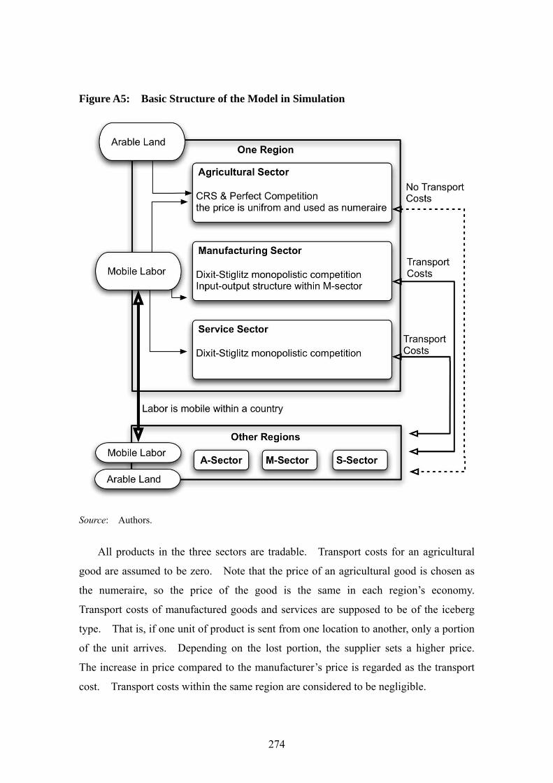
In our economic model, there are 1,715 locations, indexed by r. The basic structure

of the model is shown in Figure A5. There are two endowments: labor and arable land.

Labor is mobile within a country, but immobile among countries as Figure A5 shows.

Arable lands are unequally spread in all regions and owned by all labors of a region.

Everyone in a country is assumed to share the same tastes. Preferences are

273

described by the Cobb-Douglas function of consumption of an agricultural good, a

manufacturing aggregate and a services aggregate. The manufacturing aggregate is

expressed by a constant elasticity of substitution (CES) function of consumption of

individual manufactured goods. Likewise, the services aggregate is expressed by the

other CES function of consumption of individual services. This pertains to one mass of

varieties of manufactured goods and another mass of varieties of services. The

expenditure share of an agricultural good is meant to be so large that the agricultural good

is produced in all locations.

There are three sectors: agriculture, manufacturing, and services, and the

manufacturing sector is divided into 5 sub-sectors. As Figure A5 shows, the agricultural

sector produces a single and homogeneous good using a constant-returns technology

under conditions of perfect competition. However, manufacturing firms produce

differentiated products among a mass of varieties of manufactured goods using an

increasing-returns technology under conditions of monopolistic competition. Similarly,

differentiated services among the other mass of varieties of services are produced using

an increasing-returns technology under conditions of monopolistic competition.

Economies of scale arise at the level of variety; there are no economies of scope or of

multiplant operations. Since each firm produces or serves one variety of good, the

spread of varieties affects the available size of inputs in each region. Inputs for

agricultural products are labor and arable land, inputs for manufactured goods are labor

and manufacturing aggregate, and input for services consist only of labor. That is,

manufacturing firms use input-output structures, but services do not have such structures.

Manufacturing intermediaries are procured from all manufacturing firms. As for labor,

this sector does not have sector-specific labor; thus, labor moves to the sectors that offer

higher nominal wage rates in the region.

274

Figure A5: Basic Structure of the Model in Simulation

Source: Authors.

All products in the three sectors are tradable. Transport costs for an agricultural

good are assumed to be zero. Note that the price of an agricultural good is chosen as

the numeraire, so the price of the good is the same in each region’s economy.

Transport costs of manufactured goods and services are supposed to be of the iceberg

type. That is, if one unit of product is sent from one location to another, only a portion

of the unit arrives. Depending on the lost portion, the supplier sets a higher price.

The increase in price compared to the manufacturer’s price is regarded as the transport

cost. Transport costs within the same region are considered to be negligible.

275

A2-3. The Specifications of Our Simulation Model

Our simulation model is used to determine twelve values of the following regional

variables: nominal wage rates in three sectors; land rent, regional income; regional

expenditure on manufactured goods, price index of manufactured goods and of services;

average real wage rates in three sectors, population share of a location in a country and

population shares of a sector in three industries within one location. The dynamics of

labor are decided by three differential equations. We start from the specification of the

equation, which determines each variable under a given distribution of labor, and then we

explain the dynamics of labor selection working within a sector in a location.

A2-3-1. Wage Equation in Agriculture Sector

Nominal wage rates in the agriculture sector are derived from cost minimization in

the agriculture sector subject to the production function of the agriculture sector

, (2.1)

where is the efficiency of production at location r; represents the labor

inputs of the agriculture sector at location r; and is the area of arable land at

location r. Since the price of an agricultural good is the same in all locations, nominal

wage rates in the agriculture sector in location r, which is expressed as , are the

value of the marginal product for labor input as follows:

(2.2)

When used with the production amount, land rents are not used explicitly.

A2-3-2. Regional Income

Regional incomes in the NEG model correspond to regional GDPs in our simulations.

Supposing that revenues from land at location r belong to households at location r, GDP

at location r is expressed as follows:

(2.3)

1)()()()( rFrLrArf AAA

)(rAA )(rL A

)(rF

)(rw A

1

)(

)()()(

rL

rFrArw

AAA

)()()()()()( rLrwrfrLrwrY SSAMM

276

where and are, respectively, nominal wage rates in the manufacturing

sector7 and the services sector at location r, and and are labor input of

the manufacturing sector and the services sector at location r, respectively.

A2-3-3. Regional Expenditure on Manufactured Goods in the Manufacturing Sector

Regional expenditure on manufactured goods at location r, which is expressed as

, consists of household purchases as final consumption and manufacturing firms as

intermediary consumption:

(2.4)

where is the consumption share of expenditures on manufactured goods and is the

input share of labor in output. Thus, the first term in (2.4) shows expenditure on

manufactured goods, and the last term in (2.4) expresses the expenditure on manufactured

goods as an intermediary purchase since shows the share of intermediary

purchases in the output of manufacturing firms.

A2-3-4. The Price Index of Manufactured Goods in the Manufacturing Sector

The price index of manufactured goods at location r is expressed as follows:

(2.5)

where stands for the iceberg transport costs from location r to location s for

manufactured goods and is the elasticity of substitution between any two

differentiated manufactured goods. To derive (2.5), we substitute the price of

manufactured goods and the number of varieties with the minimum cost of purchasing a

unit of the manufacturing aggregate. Manufacturing firms at location r produce using

the composite of labor and manufacturing aggregate. The technology for the composite

7 In the actual model, the manufacturing sector is divided into 5 sub-sectors. So, the subscript M

consists of M1 to M5. For simplicity, these subsectors are represented as a group by the “Manufacturing” sector in this description

)(rwM )(rwS

)(rLM )(rLS

)(rE

)()(1

)()( rLrwrYrE MMM

M

1

)1(

1

1

)1()1()1(1 )()()()()(

MMMMM

R

s

MrsMMMMM TsGswrAsLrG

MrsT

M

277

requirements is the same for all varieties and in all locations and is expressed as a linear

function of production quantity with a fixed input requirement. The price of

manufactured goods is set as where is the

nominal wage of the manufacturing sector at location r, and is the price index of

manufactured goods at location r. Here, the marginal input requirement is supposed to

equal to the price-cost markup. The supply of a variety is decided by the zero-profit

condition. The quantity of supply depends on the size of the fixed input requirement.

Using the supply of manufactured goods and choosing the size of the fixed input

requirement adequately, the number of manufacturing firms at a location is determined by

using the relation between the share of labor input and the demand for manufactured

goods. As a first step, the price index of manufactured goods is derived from the

expenditure minimization of a constant-elasticity-of-substitution function.

A2-3-5. The Price Index of Services

The price index of services at location r is expressed as follows:

(2.6)

where is the iceberg transport costs from location r to location s, for services,

is the elasticity of substitution between any two differentiated services. We choose the

production units of a firm that equals the inverse of the consumption share of services.

Note that the derivation processes are slightly different. Using only labor, the

technology is the same for all varieties and in all locations is expressed as a linear

function of production quantity with a fixed input requirement. The price of services

is set as where is the nominal wage of the service

sector at location r and is the production efficiency of the service sector at

location r. The number of varieties of services is decided from the equality of wage

payment and the expenditure share of labor at location r.

)(/)()()( 1 rArGrwrp MMMM )(rwM

)(rGM

GS (r) LS (s)AS (r) S 1wS (s)( S 1)TrsS( S 1)

s1

R

1

( S 1)

SrsT S

)(/)()( rArwrp SSS )(rwS

)(rAS

278

A2-3-6. Nominal Wages in the Manufacturing Sector

Nominal wages in the manufacturing sector at location r at which firms in each

location break even is expressed as follows:

, (2.7)

using the equality of demand and supply on a variety of manufactured goods.

A2-3-7. Nominal Wages in the Service Sector

Similarly, nominal wages in the service sector at location r are expressed as follows:

. (2.8)

A2-3-8. The Dynamics of Labor Migration among Sectors in a Region

From (2.1) to (2.8), the variables are decided using a given configuration of labor.

Derived regional GDP, nominal wage rates, and price indexes are used to determine

labor’s decision on a working sector and place. The dynamics for labor to decide on a

specific sector within a location is expressed as follows:

, , (2.9)

where is the change in labor (population) share for a sector within a location, is

the parameter used to determine the speed of switching jobs within a location, is

the real wage rate of any sector at location r, and is the average real wage rate at

location r. The population share for a sector within a country is expressed as follows:

.

wM (r) AM (r)

1

M E(s)s1

R

TrsM 1 M GM (s)(1 M )

1

M

GM (r)1

1

wS (r) AS (r) Y (r)TrsS1 S

s1

R

GS (s)(1 S )

1

S

I (r) I

I (r)

(r)1

I (r)

I {A, M,S}

)(rI I

)(rI

)(r

I (r) LI (r)

LA (r) LM (r) LS(r)

279

A2-3-9. Dynamics of Labor Migration between Regions

The dynamics of labor migration between regions is expressed as follows:

(2.10)

where is the change in the labor (population) share of a location in a country,

is the parameter for determining the speed of migration between locations, and is

the population share of a location in a country. In (2.10), shows the real wage rate

of a location and is specified as follows:

,

where shows the consumption share of services. Furthermore, in (3.10)

shows the average real wage rate at location r.

Notice that labor migration is affected by per capita regional GDP and price index.

Using two dynamics, (2.9) and (2.10), we decided the spread of labor among locations

and the selection of sectors in a location.

A3. PARAMETERS

A3-1. Consumption Share

The Consumption share of consumers by industry is uniformly determined for the

entire region in the model. It would be more realistic to change the share by country or

region, however at this time we do not have enough reliable consumption data. The

consumption share by industry is identical to the GDP share by industry for the entire

region as shown in Table A1.

L (r) L

(r)

C

1

L (r)

)(rL L

)(rL

)(r

(r) Y(r) /(LA (r) LM (r) LS(r))

GM (r)GS(r)

C

280

Table A1: Consumption Share by Industry

Consumption Share

Agriculture 0.08002

Automotive 0.02323

E&E 0.02007

Textile & Garment 0.02429

Food Processing 0.03228

Other Manufacturing 0.17286

Services 0.64697

Source: Authors.

A3-2. Labor Input Share

The labor input share for each industry is uniformly determined for the entire region

in the model, according to that of Thailand in the year 2000 as taken from International

Input Output table by IDE. We could differentiate the value by country, according to the

I-O Table, but we have avoided it intentionally. Due to the fact that the simulation is run

for more than 20 years, it is not realistic to fix the labor input share for such a long period

of time, especially for a developing country. We do not have the methodology to change

the share with confidence, so we decided to use an “average” value, in this case, that of

Thailand as a country at the middle-stage of economic development. The labour input

share is shown in Table A2. Please note that the labour input share is calculated by 1 –

(value of intermediate input share).

Table A2: Labor input share by industry

Labor Input Share

Agriculture 0.633

Automotive 0.621

E&E 0.633

Textile & Garment 0.654

Food Processing 0.796

Other Manufacturing 0.733

Services 1.000

Source: Authors.

A3-3. Product Differentiation (Sigma)

We adopt the elasticity of substitution for manufacturing sectors from Hummels

(1999) and estimate that for services as follows: 5.1 for Food, 8.4 for Textile, 8.8 for

281

Electronics, 7.1 for Transport, 5.3 for Other manufacturing, and 5.0 for Services. The

estimates for the elasticity for services are obtained from the estimation of the usual

gravity equation for services trade, including importer’s GDP, exporter’s GDP, importer’s

corporate tax, geographical distance between countries, a dummy of free trade agreement,

a linguistic commonality dummy, and the colonial dummy as independent variables.

The elasticity for services is obtained from the transformation of a coefficient for the

corporate tax because it directly changes services’ prices. For this estimation, we mainly

employ the data from “Organisation for Economic Co-operation and Development

(OECD) Statistics on International Trade in Services”.8

A3-4. Transport Costs

This subsection explains how transport costs between regions are calculated. We

first estimate the multinomial logit model on firms’ behavior in shipping their products by

using firm-level data. Next, we estimate some parameters such as holding time across

borders. By employing these estimates in addition to the multinomial logit results, we

can specify a transport costas a function for calculating the transport costs between

regions. After that, we estimate Policy and Cultural Barriers (PCBs). Finally, we arrive

at the transport costs between regions to be used in the simulation.

A3-4-1. Firm-level Transportation Modal Choice

This section estimates the following model in which firms choose a transportation

mode from among the following three: air, sea, and land:

(3.1)

where εM denotes unobservable mode characteristics, while Abroadji takes unity if regions

i and j belong to different countries and zero otherwise; dji is the geographical distance

8 The use of OECD data has two kinds of shortcomings. The first one is that the services trade statistics in the OECD database are based on balance-of-payments, which primarily covers modes 1 and 2. This implies that our estimate is based on a quite-limited part of services. Second, trade data between non-OECD countries are not widely available. Thus, our use of the OECD database does not include almost all trade among our GSM sample countries. In other words, our estimation is valid only when we assume that the elasticity of substitution in services is almost same between developed countries (OECD countries) and developing countries (GSM countries).

,ln Mk kMks jis

MsjiMMM vduAbroadUV

282

between regions i and j. us is industry dummy. When εM is independent and follows the

identical type I extreme value distribution across modes, the probability that the firm

chooses mode M is given by:

for M = Air, Sea, Truck. (3.2)

The coefficients are estimated by maximum likelihood procedures. In other words,

a multinomial logit (MNL) model is used to estimate the probability that a firm chooses

one of the three transportation modes: air, sea, and truck. In the following, truck is a

base mode.

The geographical distance affects firms’ modal choices through not only a per-unit

physical charge for shipments but also shipping time costs due to the nature of demand

for shipments. Transportation time has a larger influence on the price of products that

decay rapidly over time; for example, time-sensitive products include perishable goods

(fresh vegetables), new information goods (newspapers) and specialized intermediate

inputs (parts for Just In Time production). A lengthy shipping time may lead to a

complete loss of commercial opportunity for products and their components, which is

more likely to be significant for goods with a rapid product life cycle and high demand

volatility. Given the value of timeliness in selling a product, time costs are small for

timely shipments (short transport time). In other words, time costs will be the highest

for shipping by sea and the lowest for shipping by air. On the other hand, the physical

transport costs will be highest for air and the lowest for sea. Truck transport will have

a medium level of costs comparing air and sea transport. As a result, the coefficient

for the geographical distance represents the (average) difference in the sum of the above

two kinds of transport costs (time and physical transportation) per distance between

truck and air/sea.

Furthermore, three points are noteworthy. Firstly, as mentioned above, shipping

time costs obviously differ among industries. Such differences among industries are

controlled by introducing the intercepts of industry dummy variables (us) with distance

variables. Secondly, the level of port infrastructure is obviously different among

countries. This yields different impacts of the aforementioned two kinds of transport

SeaTruckAir

M

UUU

U

jijiieee

edAbroadMY

1ln,|Pr

283

costs among shipping countries. To control such differences among countries in which

reporting firms locate, we introduce country dummy variables (vk). Lastly, qualitative

differences between intra- and international transactions are controlled by introducing a

binary variable (Abroad), taking unity if transactions are international ones and zero if

otherwise.

Our main data source is the Establishment Survey on Innovation and Production

Network for selected manufacturing firms in four countries in East Asia for 2008 and

2009 (Table A3). The four countries covered in the survey were Indonesia, the

Philippines, Thailand and Vietnam. The sample population is restricted to selected

manufacturing hubs in each country (JABODETABEK area, i.e., Jakarta, Bogor, Depok,

Tangerang, and Bekasi, for Indonesia; CALABARZON area, i.e., Cavite, Laguna,

Batangas, Rizal, and Quezon, for the Philippines; Greater Bangkok area for Thailand;

and Hanoi area and Ho Chi Minh City for Vietnam). This dataset includes information

on the mode of transport that each firm chooses in supplying its main product and

sourcing its main intermediate inputs. From there, the products’ origin and destination

can be also identified. In our analysis, however, the combination between origin and

destination is restricted to one accessible by land transportation.

Let’s take a brief look at a firms’ choice of transportation mode. Table A3 reports

the combination of trading partners in our dataset. There are three noteworthy points

here. Firstly, as mentioned above, firms in the Philippines and Indonesia are restricted

to the ones with intranational transactions, although most of the firms in the other

countries in our dataset are also engaged in intranational transactions. Secondly, there

are a relatively large number of Vietnamese firms trading with China. Third, Table A4

shows the transportation mode by the location of firms, indicating that most of our

sample firms tend to choose truck. Intuitively, this may be consistent with the first fact

that most of the firms trade domestically.

284

Table A3: The Combination of Trading Partners in the Dataset

Indonesia Philippines Thailand Vietnam

Cambodia 1

China 6 52

Hong Kong 5

Indonesia 449

Malaysia 2

Myanmar 1

Philippines 254

Singapore 2

Thailand 151 7

Vietnam 382

Source: The Establishment Survey on Innovation and Production Network.

Table A4: The Chosen Transportation Mode by Location of Firms Indonesia Philippines Thailand Vietnam

Air 19 7 2 11

Sea 17 11 6 51

Truck 413 236 150 389

Source: The Establishment Survey on Innovation and Production Network.

The MNL result is provided in Table A5. There are three noteworthy points.

Firstly, in trading with partners abroad, firms are likely to choose air or sea. Secondly,

the coefficients for distance are estimated to be significantly positive, indicating that the

larger the distance between trading partners, the more likely the firms are to choose air

or sea. Specifically, this result implies that the two kinds of transport costs per

distance are lower in air and sea than in truck. Third, the intercept term of distance in

machinery industries has a significantly positive coefficient for air. This result may

indicate the large amount of time costs in the machinery industry.

285

Table A5: Result of Multinomial Logit Analysis

Truck as a basis Air Sea

Coef. S.D. Coef. S.D.

Abroad 3.573 *** 0.736 2.915 *** 0.428

ln Distance (Food as a basis) 0.444 *** 0.170 1.268 *** 0.167

*Textiles 0.104 0.126 -0.151 0.094

*Machineries 0.300 ** 0.135 0.112 0.086

*Automobile 0.201 0.174 -0.104 0.154

*Others 0.148 0.106 -0.068 0.066

Constant -5.711 *** 0.760 -9.621 *** 0.993

Country dummy: Indonesia as a basis

Philippines -0.336 0.470 0.364 0.446

Thailand -2.239 ** 0.904 -0.794 0.624

Vietnam -2.483 *** 0.683 -0.437 0.419

Statistics

Observations 1,312

Pseudo R-squared 0.3407

Log likelihood -321.5

Note:***, **, and * show 1%, 5%, and 10% significance, respectively.

Lastly, we conduct some simulations to get a more intuitive picture on the

transportation modal choice. Specifically, employing our estimators, we calculate the

distance between trading partners in which the two transportation modes become

indifferent in terms of their probability. For example, suppose that a firm in the food

industry in Bangkok trades with a partner located in another city. Our calculation

reveals how far the city is from Bangkok if the probability of choosing air/sea is equal

to that of choosing truck. In the calculation, we set Abroad to the value of one, i.e.,

international transactions. The results are reported in Table A6. In Bangkok, for

example, firms in the machinery industry choose air or sea if their trading partners are

located more than 400 km away. On the other hand, firms in the food industry

basically only use truck.

286

Table A6: Probability Equivalent Distance with Truck (Kilometer): Domestic and International Transportation from Bangkok

Domestic International

Air Sea Air Sea

Food 60,300,000 3,699 19,254 371

Textiles 2,022,900 11,218 2,968 825

Machineries 44,009 1,899 361 229

Automobile 225,394 7,693 886 628

Others 684,540 5,909 1,634 520

Source: Authors’ calculation based on the MNL result in Table A5.

A3-4-2. The Estimation of Speed and Holding Time

In this section, we estimate some parameters necessary for calculating transport costs

in Section A3-4-3. Specifically, we estimate transportation speed and holding time. Our

strategy for estimating those is very straightforward and simple. We regress the

following equation:

TimeijM = ρ0 + ρ1 Abroadij

M + ρ2 DistanceijM + εij

M. The coefficients ρ0

Mand ρ1Mrepresent mode M’s holding time in domestic

transportation and its additional time in international transportation, respectively. The

inverse of ρ2M indicates the average transportation speed in mode M. We use the same data

as in the previous section. However, the estimation in this section does not require us to

restrict our sample to firms with transactions between regions accessible by truck.

The OLS regression results are reported in Table A7. Although some of the holding

time coefficients, i.e., ρ0M and ρ1

M, are estimated as being insignificant, their magnitude is

reasonable enough. As for the distance coefficient, its magnitude in sea and truck is

reasonable, but that in air is disappointing and too far from the intuitive speed, say, around

800 km/h. One possible reason is that “time” in our dataset always includes the land

transportation time to airport. This will cause the air transportation speed to be

understated.

287

Table A7: Results of OLS Regression: Holding Time and Transportation Speed

Air Sea Truck

Estimation Results

Abroad 9.010 11.671 10.979***

[8.350] [13.320] [2.440]

Distance 0.018* 0.068*** 0.026***

[0.010] [0.018] [0.002]

Constant 6.123 3.301 2.245***

[7.940] [13.099] [0.739]

Holding Time (Hours)

Domestic 9.010 11.671 10.979

International 15.133 14.972 13.224

Speed (Kilometers/Hour) 55.556 14.706 38.462

Observations 51 34 754

R-squared 0.1225 0.3698 0.1772

Notes: ***, **, and * show 1%, 5%, and 10% significance, respectively. A dependent variable is transportation time.

A3-4-3. Specifying Transport Cost Function

We specify a simple linear transport cost function, which consists of physical

transport costs and time costs. We assume the behavior of the representative firm for

each industry as follows:

A representative firm in the machinery industry will make a choice between truck and

air transport and choose the mode with the higher probability in (3.2).

A representative firm in the other industries will make a choice between truck and sea

transport and choose the mode with the higher probability in (3.2).

Specifically, the transport cost in industry s by mode M between regions i and j is

assumed to be expressed as:

, (3.3)

where distij is the travel distance between regions i and j, speedM is travel speed per one

hour by mode M, cdistM is physical travel cost per one kilometer by mode M, and ctimes is

time cost per one hour perceived by firms in industry s. The parameters ttransMDom and

CostentTransshipmPhysical

IntlMij

DomMij

CostTransportPhysical

Mij

s

TimeTransportTotal

IntlMij

DomMij

M

ijMsij

ctransAbroadctransAbroadcdistdist

ctimettransAbroadttransAbroadSpeed

distC

1

1,

288

ctransMDom are the holding time and cost, respectively, for domestic transshipment at

ports or airports. Similarly, ttransMIntl and ctransM

Intl are the holding time and cost,

respectively, for international transshipment at borders, ports, or airports.

The parameters in the transport function are determined as follows. Firstly, by using

the parameters obtained from the results of Section 3.4.2 and borrowing some parameters

from the ASEAN Logistics Network Map 2008 by JETRO, we set some of the parameters

in the transport function as in Table A8. Notice that our estimates of SpeedAir and

ttransAirIntl in Table A8 went beyond our expectations. Thus, we set SpeedAir at the usual

level (800 km/h) and we made ttransAirIntl consistent with the ASEAN Logistics Network

Map 2008.

Secondly, after substituting those parameters for the equation (3.3) under domestic

transportation, Cijs,M becomes a function of distij and ctimes. To meet the

above-mentioned assumptions on firms’ behavior, we add the following conditions:

Table A8: Parameters from Estimation and ASEAN Logistics Network Map 2008

Truck Sea Air Unit Source

cdistM 1 0.24 45.2 US$/km Map

SpeedM 38.5 14.7 800 km/hour Table 5

ttransMDom 0 11.671 9.01 hours Table 5

ttransMIntl 13.224 14.972 12.813 hours Table 5 & Map

ctransMDom 0 190 690 US$ Map

ctransMIntl 500 N.A. N.A. US$ Map

Notes: Costs are for a 20-foot container. The parameter ctransMDom is assumed to be half of the

sum of border costs and transshipment costs in international transport from Bangkok to Hanoi. The parameters ttransM

Dom and ctransMDom for sea and air include one-time loading at

the origin and one-time unloading at the destination.

The transport cost using trucks becomes the lowest among the three modes when distij

is zero for each industry.

If the transport cost is depicted as a function of distij, a line is drawn by the function

where truck intersects with it at only one point for air and sea for the machinery

industry, and at only one point for the other industries with all non-negative distij.

Under the probability equivalent (domestic) distances in Table A6, the transport cost

Cs,Air should be equal to Cs,Truck in machineries, and Cs,Sea should be equal to Cs,Truck in

the other industries. By using this equality, we calculate ctimes for each industry as in

289

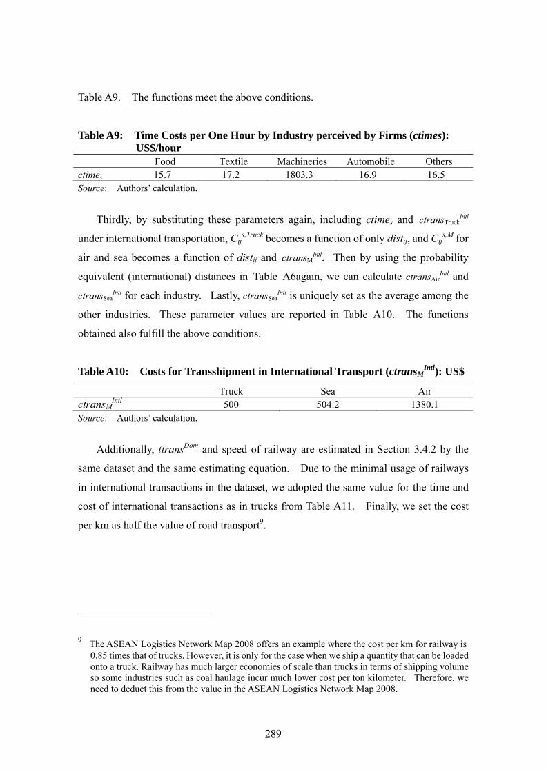
Table A9. The functions meet the above conditions.

Table A9: Time Costs per One Hour by Industry perceived by Firms (ctimes): US$/hour Food Textile Machineries Automobile Others ctimes 15.7 17.2 1803.3 16.9 16.5 Source: Authors’ calculation.

Thirdly, by substituting these parameters again, including ctimes and ctransTruckIntl

under international transportation, Cijs,Truck becomes a function of only distij, and Cij

s,M for

air and sea becomes a function of distij and ctransMIntl. Then by using the probability

equivalent (international) distances in Table A6again, we can calculate ctransAirIntl and

ctransSeaIntl for each industry. Lastly, ctransSea

Intl is uniquely set as the average among the

other industries. These parameter values are reported in Table A10. The functions

obtained also fulfill the above conditions.

Table A10: Costs for Transshipment in International Transport (ctransMIntl): US$

Truck Sea Air ctransM

Intl 500 504.2 1380.1 Source: Authors’ calculation.

Additionally, ttransDom and speed of railway are estimated in Section 3.4.2 by the

same dataset and the same estimating equation. Due to the minimal usage of railways

in international transactions in the dataset, we adopted the same value for the time and

cost of international transactions as in trucks from Table A11. Finally, we set the cost

per km as half the value of road transport9.

9 The ASEAN Logistics Network Map 2008 offers an example where the cost per km for railway is

0.85 times that of trucks. However, it is only for the case when we ship a quantity that can be loaded onto a truck. Railway has much larger economies of scale than trucks in terms of shipping volume so some industries such as coal haulage incur much lower cost per ton kilometer. Therefore, we need to deduct this from the value in the ASEAN Logistics Network Map 2008.

290

Table A11: Parameters for Rail Transport

Railway Unit Source

cdistM 0.5 US$/km Half of Truck SpeedM 19.1 km/hour Estimation ttransM

Dom 2.733 hours Estimation ttransM

Intl 13.224 hours Same as Truck ctransM

Intl 500 US$ Same as Truck Source: Authors’ calculation.

A3-4-4. Policy and Cultural Barriers (PCBs)

We explain how to quantify our measure of Policy and Cultural Barriers (PCBs). So

far, we estimate several components of transport costs including cost for Transportation

time, cost for transshipment time (holding time), physical transport cost, and physical

transshipment cost. These costs are collectively called “GSM transport cost” in this

subsection. However, some important components of the broadly defined “transport

costs” remain excluded in the model. Their examples include tariffs, non-tariff trade

barriers (e.g. quota restriction), procedures before shipping, costs arising from political

situations or some certain risks, cost arising from preference differences and cost arising

from commercial custom differences. Those costs are called PCBs, whose estimation

method is explained below. To estimate the PCBs, we employ the “log odds ratio

approach”, which is initiated by Head and Mayer (2000), in order to avoid the problem of

data availability in the estimation of the model similar to our GSM model.

The theoretical model is the same as the GSM model, except that it assumes no

inputs of consumption goods in the manufacturing sector and identical technology

among regions. Thus we state that the ratio of country j’s imports from country i in

industry s (Xijs) to those from country j (Xjj

s) can be expressed as:

ln ln ln 1 ln

The number of firms in industry s in country j is denoted by njs. Denoting the total

value of production industry s in country r and the quantity produced by each firm as

Msr and qs, respectively, we obtain Ms

r= qspsrn

sr. This is based on the assumption of

identical technology across firms and countries as noted above. Following Head and

Mayer (2000), this relationship is used to eliminate a number of firms from the

estimation equation since the appropriate data is unavailable. Thus, the above equation

291

can be written as:

ln ln ln 1 ln (3.4)

In order to avoid a simultaneity problem between Xsij and Ms

j, as in Head and Mayer

(2000), we move Msj to the LHS. The iceberg trade costs are further specified as

follows:

ln ln ln (3.5)

As a proxy for wages, we simply use GDP per capita.

By capturing PCB through coefficients for importer dummy variables, the

substitution of (3.9) into (3.8) gives us the following estimation equation:

ln ln ln

(3.6)

GDP per capitaj indicates Country j’s GDP per capita, GSM transport costijs stands

for GSM transport costs between Countries i and j in Industry s, Countryj is a dummy

variable taking unity if j is Country, and Industrys is a dummy variable taking unity if s

is Industry. To keep enough degrees of freedom, we try to obtain the

country-by-industry estimators on PCB by introducing importer dummy and industry

dummy variables separately, rather than introducing importer-by-industry dummy

variables. Furthermore, due to the data limitation, we estimate this equation only for

Thailand, the Philippines, Malaysia, and Indonesia. The data on GDP per capita are

drawn from the World Development Indicator (World Bank). The dependent variable

is constructed by employing the Asian International Input-Output Table published by the

Institute of Developing Economies (IDE).

The OLS estimation results are reported in Table A12. In order to obtain only the

estimates of PCB, we need to conduct some manipulation because PCBs are included in

a logarithmic form and the importer dummy coefficients include the elasticity of

substitution. For example, the tariff equivalent of Thai PCBs in the Machinery

Industry can be calculated as exp{(γ1+δ3)}/(1-σs)}-1. Their elasticity is estimated in

Section 3.3. The estimates for all sample countries are reported in Table A13. In

292

order to obtain the estimates for the other GSM sample countries, we regress days for

customs clearance in importing (Days), of which data is drawn from the “Doing

Business Indicator” in the World Bank, on the above estimates of PCBs. Specifically,

we estimate the following equation: (γi+ δs) = a + b lnDaysi + us + uis. Using the

estimates of a, b, industry dummy coefficients and substituting Days for each of the

remaining countries, we can get the predicted values for dependent variables for all

countries. As a result, tariff equivalents of PCBs in the other GSM countries are

provided as in Table A14.

Table A12: Estimation Results: Log Odds Ratio Equation

Coef. Std. Err.

GDP per capita ratio 0.432 0.204 ** GSM Transport cost ratio -0.134 0.136 Malaysia 1.791 0.450 *** Philippines 0.856 0.423 ** Thailand 1.584 0.395 *** Textile 0.630 0.421 Machinery 3.198 0.421 *** Automobile 0.045 0.421 Others 1.373 0.421 *** Constant -6.319 0.469 *** Adjusted R-squared 0.5433 Observations 80 Note:***, **, and * show 1%, 5%, and 10 % significant, respectively.

Table A13: Tariff Equivalents of PCBs (%)

Food Textile Machinery Automobile Others

Indonesia 162.9 42.2 105.0 326.0 189.4

Malaysia 108.6 18.6 69.4 202.0 108.5

Philippines 127.9 27.1 82.2 244.5 136.3

Thailand 144.6 34.4 93.2 282.6 161.2 Source: Authors’ estimation.

293

Table A14: Tariff Equivalents of PCBs for the Remaining Countries (%)

Food Textile Machinery Automobile Others

Bangladesh 184.7 51.3 118.9 379.5 223.9

Brunei 132.3 29.1 85.1 254.4 142.8

Cambodia 188.6 52.9 121.4 389.5 230.4

China 152.2 37.6 98.1 300.5 172.8

Hong Kong 123.4 25.2 79.3 234.3 129.7

India 204.5 59.5 131.4 430.1 256.5 Japan 91.7 11.0 58.0 166.2 84.8 Korea 97.6 13.7 62.0 178.6 93.0

Laos 185.9 51.8 119.7 382.6 225.9

Myanmar 207.9 60.9 133.5 438.9 262.1 Singapore 34.2 0.0 17.8 56.7 11.5

Vietnam 148.5 36.0 95.7 291.7 167.1 Source: Authors’ estimation.

A3-4-5. Obtaining the Transport Costs for the Simulation

Now we can obtain the transport costs between regions by industry to be used in the

simulation, using the transport cost function, several parameters, and PCBs.

Firstly, we choose the economically shortest routes between regions by industry,

adopting the transport cost function to all possible routes between regions. The shortest

routes and utilized modes may differ among industries, even in the same regional pairs.

Next, we calculate the transport costs between regions by industry. This cost is

defined as the monetary cost when shipping products by a 20-foot container. Due to the

fact that transport costs in this simulation are the ratio associated with the value of

products being shipped, we need to transform the costs to fit in the simulation. Except

for the electronics and electric appliance industries, we adopt the average values in a

20-foot container from the preliminary survey results of the FY2010 ERIA-GSM Project,

as in Table A15. As for the electronics and electric appliance industries, we assumed

firms ship 2 tons per 20-foot container. The value in 20-foot container for the electronics

and electric appliance industries is calculated independently as 376,611 USD based on the

trade value and volume data in Thailand. The reason why we adopt another value for

those industries is the fact that some electronics firms answered in the survey that they

selected mainly air transport, and that they did not utilize containers. This implies the

294

existence of a sample selection bias in this survey for those industries.

Finally, we transform the transport costs associated with the value of the products.

PCBs are multiplied by the factors shown in the equation (3.5) when the products are

imported to corresponding countries.

Table A15: Average value in 20-foot container (USD)

# of Sample Average Value

Automobile 6 89,691 E & E 11 92,746 Garment and Textile 10 34,560 Agro and Food processing 9 37,233 Others 8 59,450 Total 44

Source: Preliminary survey results of FY2010 ERIA-GSM Project.

A3-5. Technology

As proposed in subsection 3.2, the wage equation includes the variable , which

represents technology, or the productivity of each region and set by industry. is

calibrated at the beginning of the simulation to match the expected wage rate from the

wage equation and the actual wage rate. It is a kind of “residual,” including everything

that affects the wage level, other than the variables explicitly included in the wage

equation.

is basically fixed though the simulation period, but can be changed exogenously as

described in subsection 3.7.

A3-6. Speed of Adjustment

The parameters for labor mobility is set out on three levels, namely, international

labor mobility ( ), intranational (or intercity) labor mobility ( ), and inter industry

labor mobility ( ) within a region. What does γ mean? If γ=0.1, it means that a

country/region/industrywith two times higher real wages than the average attracts 10

percent labor inflow a year.

Set =0. This means that the international migration of labor is prohibited.

Although this looks like a rather extreme assumption, it is reasonable enough, taking

N C

I

N

295

into account the fact that most ASEAN countries strictly control incoming foreign labor.

Set =0.02. This means that a region with two times higher real wages than the

national average induces 2 percent labor inflow a year.

Set =0.05, too. This means that an industrial sector with two times higher real

wages than the average in the region induces 5 percent labor inflow from other

industrial sectors a year.

A3-7. Exogenous Growth Parameters

One of the important topics in constructing a realistic simulation model is how to

incorporate economic growth into the NEG model. These models are known as NEGG

(new economic geography and growth) models, such as in Baldwin and Forslid (2000).

The authors incorporated the capital production sector (knowledge) into the typical CP

model, and found that periphery industries are relatively better off by agglomeration,

although they benefit from the overall growth of the economy in some cases as well.

However, the NEGG model is an analytical model that is not easy to apply to realistic

simulations.

Without incorporating a “growth engine” sector in the model, there are two sources of

endogenous growth in the IDE-GSM model, assuming the technology is different in each

region and fixed throughout the simulation period. The first source of growth is

migration from a rural area, in which the level of technology is generally low, to an urban

area, in which the level of technology is generally high. This causes an increase in

output in the urban areas that is greater than the decrease in output in the rural areas. The

second source of growth is inter-industry migration within a region, from an industry in

which the level of technology is generally low, to another industry in which the level of

technology is generally high. This causes an increase in output in the region. These

two sources of growth are naturally extracted by the population dynamics, from lower

wage region/industry to higher wage region/industry.

In addition to the endogenous growth, there are two external sources of economic

growth. One is exogenous population growth, given the predicted rate of population

growth provided by the United Nation Population Division (Table A16). This

contributes to the endogenous economic growth.

C

I

296

The other source of growth is that technological progress coming into the region

externally. It is possible to change the level of technology, of each region arbitrarily.

However, it is difficult to set a “proper” rate of technological progress exogenously.

Therefore, the technology variable is fixed through the simulation at this moment.

Table A16: Expected Population Growth Rate (2005-2030)

Malaysia 1.47% China 0.51% Thailand 0.49% Hong Kong 0.56% Singapore 0.92% Macao 0.84% Cambodia 1.69% India 1.29% Lao PDR 1.56% Bangladesh 1.80% Myanmar 0.74% Indonesia 1.00% Vietnam 1.18% Philippines 1.66% Brunei 1.74%

Source: United Nation Population Division.

A4. DATA

A4-1. Regional Data

A4-1-1. Items

The regional data consists of the following items:

Capital City: The name of the city that represents a region, or the name of the port,

airport or railway station.

Latitude: Latitude of the city, port, airport or railway station.

Longitude: Longitude of the city, port, airport or railway station.

Region: The name of the region represented by “Capital City.” Normally, the name

of the sub-national region.

Country: The name of the country to which “Region” belongs

Habitable: take 1 if “Capital City” has population and economic activity, otherwise

take 0. The “Capital Cities” that take the value 0 is a port, airport, railway station or

city at a point of land.

Population: Total population of “Region.”

297

Employment: The number of employees of the “Region.” However, this is

identical to “Population” at this moment and not loaded into the model.

Employment A, M1 to M5, and S: The number of employees of the “Region” by

economic sector. A is agriculture. M1 is the automotive sector. M2 is the E&E

sector. M3 is the textile and garment sector. M4 is the food-processing sector. M5 is

other manufacturing sectors. S is the service sector. However, these are not loaded

into the model and most of them are proportional to GDP by sector.

GDP: nominal GRDP of “Region.”

GDP A, M1 to M5, and S: nominal GRDP of “Region” by economic sector. The

meaning of A, M1 to M5, and S are identical to those of “Employment A, M1 to

M5, and S”

Area: The area of arable rand in sq. km of “Region.”

Mining: It takes 1 if the “GDP A” of the “Region” in largely comes from mining.

Otherwise take 0.

A4-1-2. Data Source

Bangladesh:

The data is based on three-sectors (primary, manufacturing, and service) GDP data

by state from various sources. Next, the manufacturing sector has been divided into

five subsectors using value-added data from industrial censuses conducted in 2002 and

2003.

Cambodia:

Cambodia’s GDP data is available on the national level. The Japan International

Cooperation Agency (JICA) estimated provincial income and employed labor in three

industries, namely, primary, secondary, and tertiary industries based on Cambodia’s

socioeconomic survey iCSES03-05j, conducted between 2003 and 2005. Provincial

gross value added by industries was calculated by applying the ratio of income to

national GDP. Nationwide M1 to M5 was calculated based on annual statistics

published by the appropriate authorities and used as a coefficient to divide provincial

GDP of secondary industries into five sectors.

298

China, Hong Kong, and Macau:

The GDP of the subdivisions of China’s provinces was collected from the provincial

statistical yearbook. Industrial GDP was derived using GDP to calculate the share of

the number of employees in each industry at the provincial level. These derived values

were considered as industrial GDP at the provincial level. Population and arable land

were obtained from the provincial yearbook. When the GDP of the subdivisions is not

published, provincial industrial GDP is divided by the share of the population in each

subdivisions.

Data on Hong Kong’s GDP and employment were obtained from the 2003 annual

survey of industrial production and the 2003 social and economic trends in Hong Kong.

Data used for the simulation was derived using the same procedure used for China’s

data.

The 2005 statistics yearbook was used to obtain relevant data for Macau.

However, note that only employment data in the textile industry was available. The

data used for simulations was derived in the same way as the data for China.

India:

Population data was derived from the website http://www.censusindia.gov.in/.

Population and area size data at the district level was derived from the Population

Census 2001. District GDP data was taken from the “District GDP of India, 2005-06”

by INDICUS. The manufacturing GDP for five sectors was compiled from the value

added by industry in the Indian annual survey of industry (ASI).

Japan:

The administrative division of Japan follows prefectures, cities and towns. The

geographical unit employed in GSM is the prefecture level. The number of prefectures

is 47. While there have been a number of mergers of municipalities recently, the

boundaries of the prefectures remain unaffected. Although the Japan Standardized

Industrial Classification (JSIC) is different from ISIC, it is possible to compile the data to

accommodate the use of GSM. Prefectural GDP is available in official statistics at the

30-sector level. For detailed industrial classification, Kogyo-tokei (industrial statistics

299

from Japan’s Ministry of Economy, Trade, and Industry) is utilized to obtain the GDP at

a finer industrial level.

Korea:

The administrative division of Korea is arranged into eight provinces (do), one

special autonomous province (teukbyeol jachido), six metropolitan cities (gwangyeoksi)

and one special city (teukbyeolsi). The geographical unit employed in GSM is the

provincial level comprising the above-mentioned 16 regions. The Korean Standard

Industrial Classification (KSIC) generally corresponds to ISIC rev. 3 and has 17 sectors,

60 divisions, 160 groups and 333 classes. Regional GDP data is available from Gross

Regional Domestic Product and Expenditure, and this data is officially provided. For a

detailed classification at the sector level, the industrial composition is obtained from

Survey of Business Activities and Report on Mining and Manufacturing Survey.

Lao PDR:

Provincial-level industrial statistics for Laos were obtained from several sources.

Population and value-added figures for each province were based mostly on

unpublished annual provincial reports on the implementation of their socioeconomic

plan. The provincial values added are divided at their source among three industries,

namely, agriculture, industry, and services. The value added for the industries of each

province was then used to create the value added for the five sectors by splitting them

according to the provincial share of labor in M1 to M5. The labor share in M1 to M5

for each province was calculated from the nationwide business establishment survey in

2005.

Malaysia:

Malaysia’s data is based on three-sectors (primary, manufacturing, and service) and

GDP data broken down by state has been taken from various sources. The

manufacturing sector is divided into five subsectors using value-added data from the

establishment survey provided by the Department of Statistics.

300

Myanmar:

Data consists of a national-level and three-sector GDP data and income per capita

by state is based on the Report of 1997: Household Income and Expenditure Survey,

published by the Central Statistical Organization. The manufacturing sector was

divided into five subsectors using data from Table 6.11 in Myat Thein’s (2004)

Economic Development of Myanmar.

Singapore:

We used sectoral GDP data from the economic survey of Singapore. The transport

sector was divided into automotive and others using the data provided by Singstat.

Chinese Taipei:

The latest administrative division of Chinese Taipei, implemented from December

2010, consists of 5 special municipalities, 3 provincial cities and 14 counties. However,

the data for 2005 is from 4 special municipalities, 3 provincial cities and 18 counties, and

GSM follows this administrative division. The industrial classification is completely

consistent with ISIC. Since regional GDP is not available from the national authorities,

provincial GDP by industry must be compiled from other statistical sources. For

agriculture, Report of the Agricultural and Fishery Census is utilized. Except for the

agricultural sector, Report of the Industrial, Commercial, and Service Census covers the

value added in detailed classification.

Thailand:

The data for Thailand was produced in the same way as the data for China. The

data was collected from the manufacturing industrial survey for Bangkok and the

statistical report of Changwat. Data from the following provinces were also obtained:

Chonburi(1999); Ayutthaya, Chaiyaphum, Chanthaburi, Chiangrai, Chumphon, Krabi,

Lopburi, Mae Hong Son, Mukudahan, Nan, Songkhla, Yala, and Yasothon(2000);

NakhonPanom(2002); NakhonRatchasima(2005); other provinces (2001). Some

provincial data did not separate automotive industries from transport equipment, but the

data on transport equipment was also used for automobiles. A small number of

establishments in specific industries might be included in the group “others.”

301

Vietnam:

Vietnam’s data is based on three-sectors (primary, manufacturing, and service) GDP

data by state from various sources. The manufacturing sector was divided into five

subsectors using value-added data from an establishment survey.

A4-1-3.Basic Statistics

The statistics summary for 1,654 regions is provided in Table A17.

Table A17: Summary Statistics of Regions

Mean Median Min Max Population (person) 1,881,000 1,232,000 260 27,980,000 GDP (mil. USD) 5,719.0 807.6 0.3346 845,000 Arable Land (sq. km)

5,746 2,381 1 417,800

Figures A6 to A7 are the distribution of population and economic activity in 2005.

Figures A8 to A11 show GDP density per square km by industry.

302

Figure A6: Nominal GDP per capita by region (2005)

Figure A7: GDP Density (2005)

303

Figure A8: GDP Density (2005): Automotive Industry

Figure A9: GDP Density (2005): Electronics Industry

304

Figure A10: GDP Density (2005): Garment & Textile Industry

305

Figure A11: GDP Density (2005): Food Processing Industry

A4-2. Logistic Data

A4-2-1. Data Items

At this moment, the route A to B and the route B to Aare treated as identical. If both

are included in the data, the latter is used. The Logistic Data consists of following items:

Start: the name of “Capital City” at the start point of the route.

End: the name of “Capital City” at the end point of the route.

Name: The name of the route. Take “NA” if not available or unknown.

Distance: The distance of the route. If it takes -1, the slant distance between “Start”

and “End” cities are automatically calculated.

Speed: The speed of the vehicle running on the route. If it takes -1, the speed of

the vehicle is set based on “Quality” and “Mode” of transport, according to the

table included in the model (See Table A18).

Border: It takes 1 if the land/railway route goes through the national border(s). In

case of air and sea routes, take 1 if “Start” and “End” cities belong different country,

i.e., the route is international. Otherwise takes 0.

Overhead: It takes -1 normally. If “Border” then 1, the overhead TIME going

through the national border is specified. Or If “Mode” is not 0 (land transport),

some overhead TIME of transshipment is set, according to Table A19, typically.

Loading: It takes -1 normally. If “Border” then 1, the money costs going through

the national border is specified. Or If “Mode” then it is not 0 (land transport),

some overhead money costs of transshipment is set, according to Table A19,

typically.

Mode: 0 means land transport. 1 means sea transport. 2 means air transport. 3

means railway transport.

Quality: It takes 1 to 4, from lower to higher quality of the route. It affects the

speed of the vehicle going through the route (See Table A18). -1 equivalents to the

default value, 3, at this moment. In case of the land transport, “Quality” means

the quality of the road, literally. In case of other mode of transport, it is affected

by various factors, like the frequency of the transport service.

306

Table A18: Default Speed of Vehicle by Mode and Route quality(km/h)

Quality＼Mode 0 (land) 1(sea) 2(air) 3(railway)

1 4.0 4.0 400 10 2 19.25 7.35 400 19.1* 3 38.5* 14.7* 800* 40 4 60.0 29.4 1200 100 Note: * is the typically used value. Source: Authors.

Table A19: Overhead Time and Loading Costs by mode of transport

Overhead (hours) Loading

Land Domestic 0 0 International 13.224 500

Sea Domestic 11.671 190 International 14.972 504.2

Air Domestic 9.01 287.5 International 12.813 575.6

Rail Domestic 2.733 0 International 13.224 500

Source: Authors.

A4-2-2. Data Source

The land routes between cities are based mainly on the “Asian Highway” database of

the United Nations Economic and Social Commission for Asia and the Pacific

(UNESCAP). The actual road distance between cities is used; if road distances are not

available, slant distance is employed. Air and sea routes are compiled from the data set

assembled by the team of the Logistics Institute - Asia Pacific (TLIAP), and 535 sea

routes and 332 air routes are selectively included in the model at this moment. The

railway data is adopted from various sources, such as maps and the official websites of

railway companies.

307

REFERENCES

Anderson, E. James and Eric van Wincoop (2003), “Gravity with Gravitas: A Solution to the Border Puzzle,” American Economic Review.Vol.93, No.1. pp. 170-192.

Banomyong, R. S. Kumagai and I. Isono eds. (2011), Geographical Simulation Analysis for Logistics Enhancement for ASEAN, China and India, ERIA Research Project Report 2010, forthcoming.

Dixit, A. and Stiglitz, Joseph E. (1977), “Monopolistic Competition and Optimum Product Diversity,” The American Economic Review, Vol.67, No.3. pp. 297-308.

Fujita, Masahisa, Paul Krugman, and Anthony J. Venables (1999), The SpatialEconomy: Cities, Regions, and International Trade. Cambridge, MA: MITPress.

Head, K. and Mayer, T. (2000), “Non-Europe: The Magnitude and Causes of Market Fragmentation in Europe,”WeltwirschaftlichesArchiv, Vol.136, pp. 285-314.

Hummels, D. (1999), “Toward a geography of trade costs,” GTAP Working Paper No. 17.

Kumagai, S., T. Gokan, I. Isono, and S. Keola (2008), “Geographical Simulation Model for ERIA,” in International Infrastructure Development in East Asia, ed. Nagesh Kumar, ERIA Research Project Report 2007 No.2.

Kumagai, S., T. Gokan, I. Isono, and S. Keola (2009), “The Second Generation of Geographical Simulation Model: Predicting the Effects of Infrastructure Development by Industry,” in Development of Regional Production and Logistic Networks in East Asia, ed. KittiLimskul, ERIA Research Project Report 2008 No. 4-1.

Kumagai, S., T. Gokan, I. Isono, K. Hayakawa and S. Keola (2010), Geographical Simulation Analysis for Logistic Enhancement in East Asia, ERIA Research Project Report 2009 No.7-2.

Kumagai, S., T. Gokan, I. Isono, K. Hayakawa, K. Tsubota and S. Keola (2011), “IDE/ERIA-GSM v4.0” in Geographical Simulation Analysis for Logistics Enhancement for ASEAN, China and India, Banomyong R., S. Kumagai and I. Isono eds., ERIA Research Project Report 2010, forthcoming.

Kumagai, S., T. Gokan, I. Isono, K. Hayakawa, K. Tsubota and S. Keola (2012), IDE/ERIA-GSM v5.0, ERIA Research Project Report 2011, forthcoming.

Ottaviano, Gianmarco and Jacques-F., Thisse (2005), “New Economic Geography: What about the N?,”Environment and Planning, Vol. 37, No.10, pp. 1707-1725.