chapter 6 continuous distributions

C H A P T E R 6

Continuous Distributions

LEARNING OBJECTIVES

The primary learning objective of Chapter 6 is to help you understand

continuous distributions, thereby enabling you to:

1. Solve for probabilities in a continuous uniform distribution

2. Solve for probabilities in a normal distribution using z scores and for the

mean, the standard deviation, or a value of x in a normal distribution

when given information about the area under the normal curve

3. Solve problems from the discrete binomial distribution using the

continuous normal distribution and correcting for continuity

4. Solve for probabilities in an exponential distribution and contrast the

exponential distribution to the discrete Poisson distribution

Sto

ckb

yte

/Gett

y I

mag

es

JWCL152_C06_178-215.qxd 9/14/09 8:09 AM 78

What is the human resource cost ofhiring and maintaining employeesin a company? Studies conducted by

Saratoga Institute,Pricewaterhouse-Coopers HumanResource Services,determined that

the average cost of hiring an employee is $3,270, and the averageannual human resource expenditure per employee is $1,554. Theaverage health benefit payment per employee is $6,393, and theaverage employer 401(k) cost per participant is $2,258.According to a survey conducted by the American Society forTraining and Development, companies annually spend an aver-age of $955 per employee on training, and, on average, anemployee receives 32 hours of training annually. Businessresearchers have attempted to measure the cost of employeeabsenteeism to an organization. A survey conducted by CCH,Inc., showed that the average annual cost of unscheduled absen-teeism per employee is $660. According to this survey, 35% of allunscheduled absenteeism is caused by personal illness.

Managerial and Statistical Questions

1. The survey conducted by the American Society forTraining and Development reported that, on average,

an employee receives 32 hours of training per year.Suppose that number of hours of training is uniformlydistributed across all employees varying from 0 hoursto 64 hours. What percentage of employees receivebetween 20 and 40 hours of training? What percentage of employees receive 50 hours or more of training?

2. As the result of another survey, it was estimated that,on average, it costs $3,270 to hire an employee. Supposesuch costs are normally distributed with a standard deviation of $400. Based on these figures, what is theprobability that a randomly selected hire costs more than$4,000? What percentage of employees is hired for lessthan $3,000?

3. The absenteeism survey determined that 35% of allunscheduled absenteeism is caused by personal illness. If this is true, what is the probability ofrandomly sampling 120 unscheduled absences and finding out that more than 50 were caused by personalillness?

Sources: Adapted from: “Human Resources Is Put on Notice,” WorkforceManagement, vol. 84, no. 14 (December 12, 2005), pp. 44–48. Web sites fordata sources: www.pwcservices.com/, www.astd.org, and www.cch.com

179

The Cost of Human Resources

Whereas Chapter 5 focused on the characteristics and applications of discrete distribu-tions, Chapter 6 concentrates on information about continuous distributions.Continuous distributions are constructed from continuous random variables in whichvalues are taken on for every point over a given interval and are usually generated fromexperiments in which things are “measured” as opposed to “counted.” With continuousdistributions, probabilities of outcomes occurring between particular points are deter-mined by calculating the area under the curve between those points. In addition, theentire area under the whole curve is equal to 1. The many continuous distributions in statistics include the uniform distribution, the normal distribution, the exponential dis-tribution, the t distribution, the chi-square distribution, and the F distribution. Thischapter presents the uniform distribution, the normal distribution, and the exponentialdistribution.

THE UNIFORM DISTRIBUTION6.1

The uniform distribution, sometimes referred to as the rectangular distribution, is a relatively simple continuous distribution in which the same height, or f (x), is obtainedover a range of values. The following probability density function defines a uniform distribution.

JWCL152_C06_178-215.qxd 7/23/09 7:31 AM Page 179

http://www.pwcservices.com/

http://www.astd.org

http://www.cch.com

180 Chapter 6 Continuous Distributions

Figure 6.1 is an example of a uniform distribution. In a uniform, or rectangular, dis-tribution, the total area under the curve is equal to the product of the length and the width ofthe rectangle and equals 1. Because the distribution lies, by definition, between the x values ofa and b, the length of the rectangle is (b - a). Combining this area calculation with the factthat the area equals 1, the height of the rectangle can be solved as follows.

But

Therefore,

and

These calculations show why, between the x values of a and b, the distribution has a con-stant height of 1 (b - a).

The mean and standard deviation of a uniform distribution are given as follows.>

Height =

1

(b - a)

(b - a)(Height) = 1

Length = (b - a)

Area of Rectangle = (Length)(Height) = 1

f(x)

xa b

Area = 1

1b – a

Uniform Distribution

FIGURE 6.1

PROBABILITY DENSITYFUNCTION OF A UNIFORMDISTRIBUTION

f (x) = L1

b - afor a … x … b

0 for all other values

MEAN AND STANDARDDEVIATION OF A UNIFORMDISTRIBUTION

s =

b - a

112

m =

a + b

2

Many possible situations arise in which data might be uniformly distributed. As anexample, suppose a production line is set up to manufacture machine braces in lots of fiveper minute during a shift. When the lots are weighed, variation among the weights isdetected, with lot weights ranging from 41 to 47 grams in a uniform distribution. Theheight of this distribution is

f (x) = Height =

1

(b - a)=

1

(47 - 41)=

1

6

JWCL152_C06_178-215.qxd 7/23/09 7:31 AM Page 180

6.1 The Uniform Distribution 181

The mean and standard deviation of this distribution are

Figure 6.2 provides the uniform distribution for this example, with its mean, standard devi-ation, and the height of the distribution.

Determining Probabilities in a Uniform Distribution

With discrete distributions, the probability function yields the value of the probability. Forcontinuous distributions, probabilities are calculated by determining the area over aninterval of the function. With continuous distributions, there is no area under the curve fora single point. The following equation is used to determine the probabilities of x for a uni-form distribution between a and b.

Standard Deviation =

b - a

112=

47 - 41

112=

6

3.464= 1.732

Mean =

a + b

2=

41 + 47

2=

88

2= 44

f(x)

x41 47

16

μ = 44σ = 1.732(Weights)

Distribution of Lot Weights

FIGURE 6.2

PROBABILITIES IN AUNIFORM DISTRIBUTION

where:a … x1 … x2 … b

P(x) =

x2 - x1

b - a

Remember that the area between a and b is equal to 1. The probability for any intervalthat includes a and b is 1. The probability of x b or of x a is zero because there is noarea above b or below a.

Suppose that on the machine braces problem we want to determine the probabilitythat a lot weighs between 42 and 45 grams. This probability is computed as follows:

Figure 6.3 displays this solution.The probability that a lot weighs more than 48 grams is zero, because x = 48 is greater

than the upper value, x = 47, of the uniform distribution. A similar argument gives theprobability of a lot weighing less than 40 grams. Because 40 is less than the lowest value ofthe uniform distribution range, 41, the probability is zero.

P(x) =

x2 - x1

b - a=

45 - 42

47 - 41=

3

6= .5000

…Ú

JWCL152_C06_178-215.qxd 7/23/09 7:31 AM Page 181


f(x)

x41 47Weight (grams)

42 45

.5000

Solved Probability in a

Uniform Distribution

FIGURE 6.3

DEMONSTRATION

PROBLEM 6.1

Suppose the amount of time it takes to assemble a plastic module ranges from 27 to

39 seconds and that assembly times are uniformly distributed. Describe the distribution.

What is the probability that a given assembly will take between 30 and 35 seconds?

Fewer than 30 seconds?

Solution

The height of the distribution is 1 12. The mean time is 33 seconds with a standard

deviation of 3.464 seconds.

>

s =

b - a

112=

39 - 27

112=

12

112= 3.464

m =

a + b

2=

39 + 27

2= 33

f (x) =

1

39 - 27=

1

12

f(x)

x27 39 = 33μ = 3.464σ

Time (seconds)

112f(x) =

There is a .4167 probability that it will take between 30 and 35 seconds to assemble

the module.

There is a .2500 probability that it will take less than 30 seconds to assemble the module.

Because there is no area less than 27 seconds, P(x 30) is determined by using only the

interval 27 x 30. In a continuous distribution, there is no area at any one point (only

over an interval). Thus the probability x 30 is the same as the probability of x 30.…6

6…

6

P (x 6 30) =

30 - 27

39 - 27=

3

12= .2500

P (30 … x … 35) =

35 - 30

39 - 27=

5

12= .4167

JWCL152_C06_178-215.qxd 7/23/09 7:31 AM Page 182

6.1 The Uniform Distribution 183

Using the Computer to Solve for UniformDistribution Probabilities

Using the values of a, b, and x, Minitab has the capability of computing probabilities forthe uniform distribution. The resulting computation is a cumulative probability from theleft end of the distribution to each x value. As an example, the probability question, P (410 x 825), from Demonstration Problem 6.2 can be worked using Minitab. Minitab com-putes the probability of x 825 and the probability of x 410, and these results are shownin Table 6.1. The final answer to the probability question from Demonstration Problem 6.2is obtained by subtracting these two probabilities:

P (410 … x … 825) = .6365 - .2138 = .4227

……

…

…

DEMONSTRATION

PROBLEM 6.2

According to the National Association of Insurance Commissioners, the average

annual cost for automobile insurance in the United States in a recent year was $691.

Suppose automobile insurance costs are uniformly distributed in the United States

with a range of from $200 to $1,182. What is the standard deviation of this uniform dis-

tribution? What is the height of the distribution? What is the probability that a person’s

annual cost for automobile insurance in the United States is between $410 and $825?

Solution

The mean is given as $691. The value of a is $200 and b is $1,182.

The height of the distribution is

The probability that a randomly selected person pays between $410 and $825 annu-

ally for automobile insurance in the United States is .4226. That is, about 42.26% of

all people in the United States pay in that range.

P (410 … x … 825) =

825 - 410

1,182 - 200=

415

982= .4226

x1 = 410 and x2 = 825

1

1,182 - 200=

1

982= .001

s =

b - a

112=

1,182 - 200

112= 283.5

f(x)

x200 1182410 825= 691μ= 283.5σ

TABLE 6.1

Minitab Output for Uniform

Distribution

CUMULATIVE DISTRIBUTION FUNCTION

Continuous uniform on 200 to 1182

x P(X = x)825 0.636456

410 0.213849

6

JWCL152_C06_178-215.qxd 9/4/09 5:11 PM Page 183


6.1 PROBLEMS 6.1 Values are uniformly distributed between 200 and 240.

a. What is the value of f (x) for this distribution?

b. Determine the mean and standard deviation of this distribution.

c. Probability of (x 230) = ?

d. Probability of (205 x 220) = ?

e. Probability of (x 225) = ?

6.2 x is uniformly distributed over a range of values from 8 to 21.

a. What is the value of f (x) for this distribution?

b. Determine the mean and standard deviation of this distribution.

c. Probability of (10 x 17) = ?

d. Probability of (x 22) = ?

e. Probability of (x 7) = ?

6.3 The retail price of a medium-sized box of a well-known brand of cornflakes rangesfrom $2.80 to $3.14. Assume these prices are uniformly distributed. What are theaverage price and standard deviation of prices in this distribution? If a price is randomly selected from this list, what is the probability that it will be between $3.00and $3.10?

6.4 The average fill volume of a regular can of soft drink is 12 ounces. Suppose the fillvolume of these cans ranges from 11.97 to 12.03 ounces and is uniformly distributed.What is the height of this distribution? What is the probability that a randomlyselected can contains more than 12.01 ounces of fluid? What is the probability thatthe fill volume is between 11.98 and 12.01 ounces?

6.5 Suppose the average U.S. household spends $2,100 a year on all types of insurance.Suppose the figures are uniformly distributed between the values of $400 and $3,800.What are the standard deviation and the height of this distribution? What proportionof households spends more than $3,000 a year on insurance? More than $4,000?Between $700 and $1,500?

Ú

6

6…

…

……

7

Probably the most widely known and used of all distributions is the normal distribution.It fits many human characteristics, such as height, weight, length, speed, IQ, scholasticachievement, and years of life expectancy, among others. Like their human counterparts,living things in nature, such as trees, animals, insects, and others, have many characteristicsthat are normally distributed.

Many variables in business and industry also are normally distributed.Some examples of variables that could produce normally distributed measure-ments include the annual cost of household insurance, the cost per square footof renting warehouse space, and managers’ satisfaction with support from

ownership on a five-point scale. In addition, most items produced or filled by machinesare normally distributed.

Because of its many applications, the normal distribution is an extremely importantdistribution. Besides the many variables mentioned that are normally distributed, the nor-mal distribution and its associated probabilities are an integral part of statistical processcontrol (see Chapter 18). When large enough sample sizes are taken, many statistics arenormally distributed regardless of the shape of the underlying distribution from whichthey are drawn (as discussed in Chapter 7). Figure 6.4 is the graphic representation of thenormal distribution: the normal curve.

NORMAL DISTRIBUTION6.2

Excel does not have the capability of directly computing probabilities for the uniformdistribution.

JWCL152_C06_178-215.qxd 8/7/09 12:11 AM Page 184

6.2 Normal Distribution 185

History of the Normal Distribution

Discovery of the normal curve of errors is generally credited to mathematician andastronomer Karl Gauss (1777–1855), who recognized that the errors of repeated measure-ment of objects are often normally distributed.* Thus the normal distribution is some-times referred to as the Gaussian distribution or the normal curve of error. A modern-dayanalogy of Gauss’s work might be the distribution of measurements of machine-producedparts, which often yield a normal curve of error around a mean specification.

To a lesser extent, some credit has been given to Pierre-Simon de Laplace (1749–1827)for discovering the normal distribution. However, many people now believe that Abrahamde Moivre (1667–1754), a French mathematician, first understood the normal distribution.De Moivre determined that the binomial distribution approached the normal distributionas a limit. De Moivre worked with remarkable accuracy. His published table values for thenormal curve are only a few ten-thousandths off the values of currently published tables.†

The normal distribution exhibits the following characteristics.

■ It is a continuous distribution.

■ It is a symmetrical distribution about its mean.

■ It is asymptotic to the horizontal axis.

■ It is unimodal.

■ It is a family of curves.

■ Area under the curve is 1.

The normal distribution is symmetrical. Each half of the distribution is a mirror imageof the other half. Many normal distribution tables contain probability values for only oneside of the distribution because probability values for the other side of the distribution areidentical because of symmetry.

In theory, the normal distribution is asymptotic to the horizontal axis. That is, it doesnot touch the x-axis, and it goes forever in each direction. The reality is that most applica-tions of the normal curve are experiments that have finite limits of potential outcomes. Forexample, even though GMAT scores are analyzed by the normal distribution, the range ofscores on each part of the GMAT is from 200 to 800.

The normal curve sometimes is referred to as the bell-shaped curve. It is unimodal inthat values mound up in only one portion of the graph—the center of the curve. The normaldistribution actually is a family of curves. Every unique value of the mean and every uniquevalue of the standard deviation result in a different normal curve. In addition, the total areaunder any normal distribution is 1. The area under the curve yields the probabilities, so thetotal of all probabilities for a normal distribution is 1. Because the distribution is symmet-ric, the area of the distribution on each side of the mean is 0.5.

Probability Density Function of the Normal Distribution

The normal distribution is described or characterized by two parameters: the mean, , andthe standard deviation, . The values of and produce a normal distribution. The den-sity function of the normal distribution is

where= mean of x= standard deviation of x= 3.14159 . . . , and

e = 2.71828. . . .p

s

m

f (x) =

1

s12p e-1>2[(x -m)>s)]2

sms

m

*John A. Ingram and Joseph G. Monks, Statistics for Business and Economics. San Diego: Harcourt Brace Jovanovich,1989.†Roger E. Kirk, Statistical Issues: A Reader for the Behavioral Sciences. Monterey, CA: Brooks/Cole, 1972.

μ X

The Normal Curve

FIGURE 6.4

JWCL152_C06_178-215.qxd 7/23/09 7:31 AM Page 185


Using Integral Calculus to determine areas under the normal curve from this function isdifficult and time-consuming, therefore, virtually all researchers use table values to analyzenormal distribution problems rather than this formula.

Standardized Normal Distribution

Every unique pair of and values defines a different normal distribution. Figure 6.5 showsthe Minitab graphs of normal distributions for the following three pairs of parameters.

1. = 50 and = 5

2. = 80 and = 5

3. = 50 and = 10

Note that every change in a parameter ( or ) determines a different normal distri-bution. This characteristic of the normal curve (a family of curves) could make analysis bythe normal distribution tedious because volumes of normal curve tables—one for eachdifferent combination of and —would be required. Fortunately, a mechanism wasdeveloped by which all normal distributions can be converted into a single distribution: thez distribution. This process yields the standardized normal distribution (or curve). Theconversion formula for any x value of a given normal distribution follows.

sm

sm

sm

sm

sm

sm

= 5σ = 5σ

= 10σ

0 10 20 30 40 50

x Values

60 70 80 90 100

Normal Curves for Three

Different Combinations of

Means and Standard

Deviations

FIGURE 6.5

z FORMULAz =

x - m

s, s Z 0

A z score is the number of standard deviations that a value, x, is above or below the mean.If the value of x is less than the mean, the z score is negative; if the value of x is more thanthe mean, the z score is positive; and if the value of x equals the mean, the associated z scoreis zero. This formula allows conversion of the distance of any x value from its mean intostandard deviation units. A standard z score table can be used to find probabilities for anynormal curve problem that has been converted to z scores. The z distribution is a normaldistribution with a mean of 0 and a standard deviation of 1. Any value of x at the mean of anormal curve is zero standard deviations from the mean. Any value of x that is one standarddeviation above the mean has a z value of 1. The empirical rule, introduced in Chapter 3, isbased on the normal distribution in which about 68% of all values are within one standarddeviation of the mean regardless of the values of and . In a z distribution, about 68% ofthe z values are between z = -1 and z = +1.

The z distribution probability values are given in Table A.5. Because it is so frequentlyused, the z distribution is also printed inside the cover of this text. For discussion purposes,a list of z distribution values is presented in Table 6.2.

Table A.5 gives the total area under the z curve between 0 and any point on the posi-tive z-axis. Since the curve is symmetric, the area under the curve between z and 0 is thesame whether z is positive or negative (the sign on the z value designates whether thez score is above or below the mean). The table areas or probabilities are always positive.

sm

JWCL152_C06_178-215.qxd 7/23/09 7:31 AM Page 186


Solving Normal Curve Problems

The mean and standard deviation of a normal distribution and the z formula and table enablea researcher to determine the probabilities for intervals of any particular values of a normalcurve. One example is the many possible probability values of GMAT scores examined next.

The Graduate Management Aptitude Test (GMAT), produced by the EducationalTesting Service in Princeton, New Jersey, is widely used by graduate schools of business in

TABLE 6.2

z Distribution

SECOND DECIMAL PLACE IN z

z 0.00 0.01 0.02 0.03 0.04 0.05 0.06 0.07 0.08 0.09

0.0 .0000 .0040 .0080 .0120 .0160 .0199 .0239 .0279 .0319 .0359

0.1 .0398 .0438 .0478 .0517 .0557 .0596 .0636 .0675 .0714 .0753

0.2 .0793 .0832 .0871 .0910 .0948 .0987 .1026 .1064 .1103 .1141

0.3 .1179 .1217 .1255 .1293 .1331 .1368 .1406 .1443 .1480 .1517

0.4 .1554 .1591 .1628 .1664 .1700 .1736 .1772 .1808 .1844 .1879

0.5 .1915 .1950 .1985 .2019 .2054 .2088 .2123 .2157 .2190 .2224

0.6 .2257 .2291 .2324 .2357 .2389 .2422 .2454 .2486 .2517 .2549

0.7 .2580 .2611 .2642 .2673 .2704 .2734 .2764 .2794 .2823 .2852

0.8 .2881 .2910 .2939 .2967 .2995 .3023 .3051 .3078 .3106 .3133

0.9 .3159 .3186 .3212 .3238 .3264 .3289 .3315 .3340 .3365 .3389

1.0 .3413 .3438 .3461 .3485 .3508 .3531 .3554 .3577 .3599 .3621

1.1 .3643 .3665 .3686 .3708 .3729 .3749 .3770 .3790 .3810 .3830

1.2 .3849 .3869 .3888 .3907 .3925 .3944 .3962 .3980 .3997 .4015

1.3 .4032 .4049 .4066 .4082 .4099 .4115 .4131 .4147 .4162 .4177

1.4 .4192 .4207 .4222 .4236 .4251 .4265 .4279 .4292 .4306 .4319

1.5 .4332 .4345 .4357 .4370 .4382 .4394 .4406 .4418 .4429 .4441

1.6 .4452 .4463 .4474 .4484 .4495 .4505 .4515 .4525 .4535 .4545

1.7 .4554 .4564 .4573 .4582 .4591 .4599 .4608 .4616 .4625 .4633

1.8 .4641 .4649 .4656 .4664 .4671 .4678 .4686 .4693 .4699 .4706

1.9 .4713 .4719 .4726 .4732 .4738 .4744 .4750 .4756 .4761 .4767

2.0 .4772 .4778 .4783 .4788 .4793 .4798 .4803 .4808 .4812 .4817

2.1 .4821 .4826 .4830 .4834 .4838 .4842 .4846 .4850 .4854 .4857

2.2 .4861 .4864 .4868 .4871 .4875 .4878 .4881 .4884 .4887 .4890

2.3 .4893 .4896 .4898 .4901 .4904 .4906 .4909 .4911 .4913 .4916

2.4 .4918 .4920 .4922 .4925 .4927 .4929 .4931 .4932 .4934 .4936

2.5 .4938 .4940 .4941 .4943 .4945 .4946 .4948 .4949 .4951 .4952

2.6 .4953 .4955 .4956 .4957 .4959 .4960 .4961 .4962 .4963 .4964

2.7 .4965 .4966 .4967 .4968 .4969 .4970 .4971 .4972 .4973 .4974

2.8 .4974 .4975 .4976 .4977 .4977 .4978 .4979 .4979 .4980 .4981

2.9 .4981 .4982 .4982 .4983 .4984 .4984 .4985 .4985 .4986 .4986

3.0 .4987 .4987 .4987 .4988 .4988 .4989 .4989 .4989 .4990 .4990

3.1 .4990 .4991 .4991 .4991 .4992 .4992 .4992 .4992 .4993 .4993

3.2 .4993 .4993 .4994 .4994 .4994 .4994 .4994 .4995 .4995 .4995

3.3 .4995 .4995 .4995 .4996 .4996 .4996 .4996 .4996 .4996 .4997

3.4 .4997 .4997 .4997 .4997 .4997 .4997 .4997 .4997 .4997 .4998

3.5 .4998

4.0 .49997

4.5 .499997

5.0 .4999997

6.0 .499999999

= 494μ x = 600 = 100σ

Graphical Depiction of the

Area Between a Score of 600

and a Mean on a GMAT

FIGURE 6.6

0 z

JWCL152_C06_178-215.qxd 7/23/09 7:31 AM Page 187


the United States as an entrance requirement. Assuming that the scores are normally dis-tributed, probabilities of achieving scores over various ranges of the GMAT can be deter-mined. In a recent year, the mean GMAT score was 494 and the standard deviation wasabout 100. What is the probability that a randomly selected score from this administrationof the GMAT is between 600 and the mean? That is,

Figure 6.6 is a graphical representation of this problem.The z formula yields the number of standard deviations that the x value, 600, is away

from the mean.

The z value of 1.06 reveals that the GMAT score of 600 is 1.06 standard deviations morethan the mean. The z distribution values in Table 6.2 give the probability of a value beingbetween this value of x and the mean. The whole-number and tenths-place portion of thez score appear in the first column of Table 6.2 (the 1.0 portion of this z score). Across the topof the table are the values of the hundredths-place portion of the z score. For this z score,the hundredths-place value is 6. The probability value in Table 6.2 for z = 1.06 is .3554. Theshaded portion of the curve at the top of the table indicates that the probability value givenalways is the probability or area between an x value and the mean. In this particular exam-ple, that is the desired area. Thus the answer is that .3554 of the scores on the GMAT arebetween a score of 600 and the mean of 494. Figure 6.7(a) depicts graphically the solutionin terms of x values. Figure 6.7(b) shows the solution in terms of z values.

z =

x - m

s=

600 - 494

100=

106

100= 1.06

P (494 … x … 600 ƒ m = 494 and s = 100) = ?

.3554

= 494μ = 100σ

(a)

x = 600

.3554

(b)

z = 1.06z = 0

Graphical Solutions to the

GMAT Problem

FIGURE 6.7

DEMONSTRATION

PROBLEM 6.3

What is the probability of obtaining a score greater than 700 on a GMAT test that has

a mean of 494 and a standard deviation of 100? Assume GMAT scores are normally

distributed.

Solution

Examine the following diagram.

P (x 7 700 ƒ m = 494 and s = 100) = ?

x > 700

= 494μ x = 700 = 100σ

JWCL152_C06_178-215.qxd 7/23/09 7:31 AM Page 188


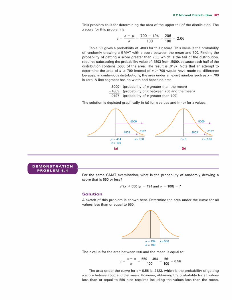
This problem calls for determining the area of the upper tail of the distribution. The

z score for this problem is

Table 6.2 gives a probability of .4803 for this z score. This value is the probability

of randomly drawing a GMAT with a score between the mean and 700. Finding the

probability of getting a score greater than 700, which is the tail of the distribution,

requires subtracting the probability value of .4803 from .5000, because each half of the

distribution contains .5000 of the area. The result is .0197. Note that an attempt to

determine the area of x 700 instead of x 700 would have made no difference

because, in continuous distributions, the area under an exact number such as x = 700

is zero. A line segment has no width and hence no area.

.5000 (probability of x greater than the mean)

-.4803 (probability of x between 700 and the mean)

.0197 (probability of x greater than 700)

The solution is depicted graphically in (a) for x values and in (b) for z values.

7Ú

z =

x - m

s=

700 - 494

100=

206

100= 2.06

DEMONSTRATION

PROBLEM 6.4

For the same GMAT examination, what is the probability of randomly drawing a

score that is 550 or less?

Solution

A sketch of this problem is shown here. Determine the area under the curve for all

values less than or equal to 550.

P (x … 550 ƒ m = 494 and s = 100) = ?

= 494μ x = 700 = 100σ

.4803

.5000

.0197

(b)(a)

z = 2.06z = 0

.4803

.5000

.0197

= 494μ x = 550 = 100σ

The z value for the area between 550 and the mean is equal to:

The area under the curve for z = 0.56 is .2123, which is the probability of getting

a score between 550 and the mean. However, obtaining the probability for all values

less than or equal to 550 also requires including the values less than the mean.

z =

x - m

s=

550 - 494

100=

56

100= 0.56

JWCL152_C06_178-215.qxd 7/23/09 7:31 AM Page 189


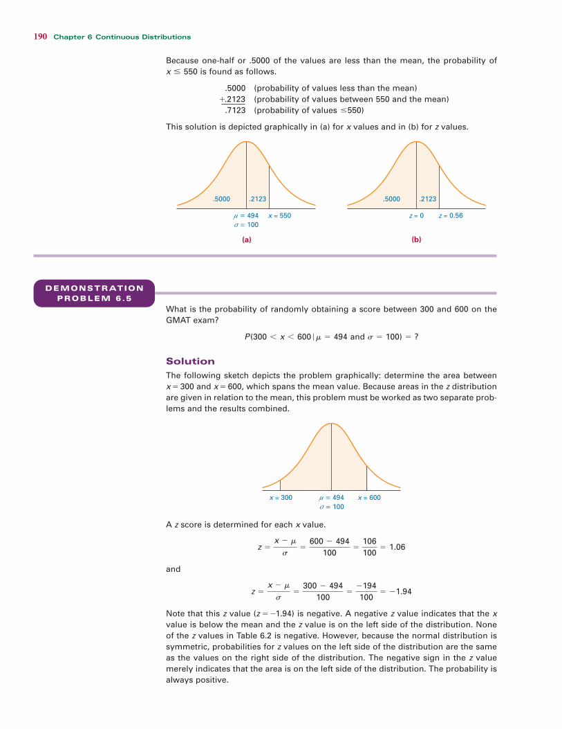
Because one-half or .5000 of the values are less than the mean, the probability of

x 550 is found as follows.

.5000 (probability of values less than the mean)

+.2123 (probability of values between 550 and the mean)

.7123 (probability of values 550)

This solution is depicted graphically in (a) for x values and in (b) for z values.

…

…

= 494μ x = 550 = 100σ

.5000 .2123

z = 0 z = 0.56

.5000 .2123

(b)(a)

DEMONSTRATION

PROBLEM 6.5

What is the probability of randomly obtaining a score between 300 and 600 on the

GMAT exam?

Solution

The following sketch depicts the problem graphically: determine the area between

x = 300 and x = 600, which spans the mean value. Because areas in the z distribution

are given in relation to the mean, this problem must be worked as two separate prob-

lems and the results combined.

A z score is determined for each x value.

and

Note that this z value (z = -1.94) is negative. A negative z value indicates that the x

value is below the mean and the z value is on the left side of the distribution. None

of the z values in Table 6.2 is negative. However, because the normal distribution is

symmetric, probabilities for z values on the left side of the distribution are the same

as the values on the right side of the distribution. The negative sign in the z value

merely indicates that the area is on the left side of the distribution. The probability is

always positive.

z =

x - m

s=

300 - 494

100=

-194

100= -1.94

z =

x - m

s=

600 - 494

100=

106

100= 1.06

= 494μx = 300 = 100σ

x = 600

P (300 6 x 6 600 ƒ m = 494 and s = 100) = ?

JWCL152_C06_178-215.qxd 7/23/09 7:32 AM Page 190


The probability for z = 1.06 is .3554; the probability for z = -1.94 is .4738. The

solution of P (300 x 600) is obtained by summing the probabilities.

.3554 (probability of a value between the mean and 600)

+.4738 (probability of a value between the mean and 300)

.8292 (probability of a value between 300 and 600)

Graphically, the solution is shown in (a) for x values and in (b) for z values.

= 494μx = 300 = 100σ

x = 600

.3554

z = –1.94 z = 1.06z = 0

.4738 .3554.4738

(b)(a)

66

DEMONSTRATION

PROBLEM 6.6

What is the probability of getting a score between 350 and 450 on the same GMAT

exam?

Solution

The following sketch reveals that the solution to the problem involves determining

the area of the shaded slice in the lower half of the curve.

In this problem, the two x values are on the same side of the mean. The areas or

probabilities of each x value must be determined and the final probability found by

determining the difference between the two areas.

and

The probability associated with z = -1.44 is .4251.

The probability associated with z = - 0.44 is .1700.

Subtracting gives the solution.

.4251 (probability of a value between 350 and the mean)

-.1700 (probability of a value between 450 and the mean)

.2551 (probability of a value between 350 and 450)

Graphically, the solution is shown in (a) for x values and in (b) for z values.

z =

x - m

s=

450 - 494

100=

-44

100= -0.44

z =

x - m

s=

350 - 494

100=

-144

100= -1.44

= 494μx = 350 = 100σx = 450

P (350 6 x 6 450 ƒ m = 494 and s = 100) = ?

JWCL152_C06_178-215.qxd 7/23/09 7:32 AM Page 191


DEMONSTRATION

PROBLEM 6.7

Runzheimer International publishes business travel costs for various cities through-

out the world. In particular, they publish per diem totals, which represent the average

costs for the typical business traveler including three meals a day in business-class

restaurants and single-rate lodging in business-class hotels and motels. If 86.65% of

the per diem costs in Buenos Aires, Argentina, are less than $449 and if the standard

deviation of per diem costs is $36, what is the average per diem cost in Buenos Aires?

Assume that per diem costs are normally distributed.

Solution

In this problem, the standard deviation and an x value are given; the object is to

determine the value of the mean. Examination of the z score formula reveals four

variables: x, , , and z. In this problem, only two of the four variables are given.

Because solving one equation with two unknowns is impossible, one of the other

unknowns must be determined. The value of z can be determined from the normal

distribution table (Table 6.2).

Because 86.65% of the values are less than x = $449, 36.65% of the per diem costs

are between $449 and the mean. The other 50% of the per diem costs are in the lower

half of the distribution. Converting the percentage to a proportion yields .3665 of the

values between the x value and the mean. What z value is associated with this area?

This area, or probability, of .3665 in Table 6.2 is associated with the z value of 1.11.

This z value is positive, because it is in the upper half of the distribution. Using the

z value of 1.11, the x value of $449, and the value of $36 allows solving for the mean

algebraically.

and

The mean per diem cost for business travel in Buenos Aires is $409.04.

m = $449 - ($36)(1.11) = $449 - $39.96 = $409.04

1.11 =

$449 - m

$36

z =

x - m

s

s

= ?μ = $36σ

x = $449

86.65%

sm

= 494μx = 350 = 100σx = 450

.4251

.2551

z = –1.44z = –0.44

z = 0

.1700

.4251

.2551

.1700

(b)(a)

JWCL152_C06_178-215.qxd 7/23/09 7:32 AM Page 192


The U.S. Environmental Protection Agency publishes figures on solid waste gen-

eration in the United States. One year, the average number of waste generated per

person per day was 3.58 pounds. Suppose the daily amount of waste generated

per person is normally distributed, with a standard deviation of 1.04 pounds. Of

the daily amounts of waste generated per person, 67.72% would be greater than

what amount?

Solution

The mean and standard deviation are given, but x and z are unknown. The prob-

lem is to solve for a specific x value when .6772 of the x values are greater than that

value.

If .6772 of the values are greater than x, then .1772 are between x and the mean

(.6772 - .5000). Table 6.2 shows that the probability of.1772 is associated with a

z value of 0.46. Because x is less than the mean, the z value actually is - 0.46. Whenever

an x value is less than the mean, its associated z value is negative and should be

reported that way.

Solving the z equation yields

and

Thus 67.72% of the daily average amount of solid waste per person weighs more

than 3.10 pounds.

x = 3.58 + (-0.46)(1.04) = 3.10

-0.46 =

x - 3.58

1.04

z =

x - m

s

= 3.58μ = 1.04σx = ?

.5000

.6772

.1772

DEMONSTRATION

PROBLEM 6.8

STATISTICS IN BUSINESS TODAY

WarehousingTompkins Associates conducted a national study of ware-housing in the United States. The study revealed manyinteresting facts. Warehousing is a labor-intensive industrythat presents considerable opportunity for improvement inproductivity. What does the “average” warehouse look like?The construction of new warehouses is restricted by pro-hibitive expense. Perhaps for that reason, the average age ofa warehouse is 19 years. Warehouses vary in size, but theaverage size is about 50,000 square feet. To visualize suchan “average” warehouse, picture one that is square with

about 224 feet on each side or a rectangle that is 500 feet by100 feet. The average clear height of a warehouse in theUnited States is 22 feet.

Suppose the ages of warehouses, the sizes of ware-houses, and the clear heights of warehouses are normallydistributed. Using the mean values already given and thestandard deviations, techniques presented in this sectioncould be used to determine, for example, the probabilitythat a randomly selected warehouse is less than 15 yearsold, is larger than 60,000 square feet, or has a clear heightbetween 20 and 25 feet.

JWCL152_C06_178-215.qxd 9/17/09 2:09 PM Page 193


Using the Computer to Solve for NormalDistribution Probabilities

Both Excel and Minitab can be used to solve for normal distribution probabilities. In each case,the computer package uses , , and the value of x to compute a cumulative probability fromthe left. Shown in Table 6.3 are Excel and Minitab output for the probability questionaddressed in Demonstration Problem 6.6: P(350 x 450 = 494 and = 100). Sinceboth computer packages yield probabilities cumulated from the left, this problem is solvedmanually with the computer output by finding the difference in P(x 450) and P(x 350).6 6

smƒ66

sm

6.2 PROBLEMS 6.6 Determine the probabilities for the following normal distribution problems.

a. = 604, = 56.8, x 635

b. = 48, = 12, x 20

c. = 111, = 33.8, 100 x 150

d. = 264, = 10.9, 250 x 255

e. = 37, = 4.35, x 35

f. = 156, = 11.4, x 170

6.7 Tompkins Associates reports that the mean clear height for a Class A warehouse inthe United States is 22 feet. Suppose clear heights are normally distributed and thatthe standard deviation is 4 feet. A Class A warehouse in the United States is randomlyselected.

a. What is the probability that the clear height is greater than 17 feet?

b. What is the probability that the clear height is less than 13 feet?

c. What is the probability that the clear height is between 25 and 31 feet?

6.8 According to a report by Scarborough Research, the average monthly householdcellular phone bill is $60. Suppose local monthly household cell phone bills arenormally distributed with a standard deviation of $11.35.

a. What is the probability that a randomly selected monthly cell phone bill is morethan $85?

b. What is the probability that a randomly selected monthly cell phone bill isbetween $45 and $70?

c. What is the probability that a randomly selected monthly cell phone bill isbetween $65 and $75?

d. What is the probability that a randomly selected monthly cell phone bill is nomore than $40?

Úsm

7sm

66sm

6…sm

6sm

…sm

TABLE 6.3

Excel and Minitab Normal

Distribution Output for

Demonstration Problem 6.6

Minitab Output

Excel Output


Normal with mean = 494 and standarddeviation = 100

x P(X <= x)

450 0.329969

350 0.074934

Prob (350 < x < 450) = 0.255035

x Value450 0.3264350 0.0735

0.2528

JWCL152_C06_178-215.qxd 7/23/09 7:32 AM Page 194

Problems 195

6.9 According to the Internal Revenue Service, income tax returns one year averaged$1,332 in refunds for taxpayers. One explanation of this figure is that taxpayerswould rather have the government keep back too much money during the year thanto owe it money at the end of the year. Suppose the average amount of tax at the endof a year is a refund of $1,332, with a standard deviation of $725. Assume thatamounts owed or due on tax returns are normally distributed.

a. What proportion of tax returns show a refund greater than $2,000?

b. What proportion of the tax returns show that the taxpayer owes money to thegovernment?

c. What proportion of the tax returns show a refund between $100 and $700?

6.10 Toolworkers are subject to work-related injuries. One disorder, caused by strains to the hands and wrists, is called carpal tunnel syndrome. It strikes as many as23,000 workers per year. The U.S. Labor Department estimates that the averagecost of this disorder to employers and insurers is approximately $30,000 perinjured worker. Suppose these costs are normally distributed, with a standarddeviation of $9,000.

a. What proportion of the costs are between $15,000 and $45,000?

b. What proportion of the costs are greater than $50,000?

c. What proportion of the costs are between $5,000 and $20,000?

d. Suppose the standard deviation is unknown, but 90.82% of the costs are morethan $7,000. What would be the value of the standard deviation?

e. Suppose the mean value is unknown, but the standard deviation is still $9,000. Howmuch would the average cost be if 79.95% of the costs were less than $33,000?

6.11 Suppose you are working with a data set that is normally distributed, with a mean of 200 and a standard deviation of 47. Determine the value of x from the followinginformation.

a. 60% of the values are greater than x.

b. x is less than 17% of the values.

c. 22% of the values are less than x.

d. x is greater than 55% of the values.

6.12 Suppose the annual employer 401(k) cost per participant is normally distributedwith a standard deviation of $625, but the mean is unknown.

a. If 73.89% of such costs are greater than $1,700, what is the mean annual employer401(k) cost per participant?

b. Suppose the mean annual employer 401(k) cost per participant is $2,258 and thestandard deviation is $625. If such costs are normally distributed, 31.56% of thecosts are greater than what value?

6.13 Suppose the standard deviation for Problem 6.7 is unknown but the mean is still 22 feet. If 72.4% of all U.S. Class A warehouses have a clear height greater than 18.5 feet, what is the standard deviation?

6.14 Suppose the mean clear height of all U.S. Class A warehouses is unknown but thestandard deviation is known to be 4 feet. What is the value of the mean clear heightif 29% of U.S. Class A warehouses have a clear height less than 20 feet?

6.15 Data accumulated by the National Climatic Data Center shows that the average windspeed in miles per hour for St. Louis, Missouri, is 9.7. Suppose wind speed measure-ments are normally distributed for a given geographic location. If 22.45% of the timethe wind speed measurements are more than 11.6 miles per hour, what is the standarddeviation of wind speed in St. Louis?

6.16 According to Student Monitor, a New Jersey research firm, the average cumulatedcollege student loan debt for a graduating senior is $25,760. Assume that the standarddeviation of such student loan debt is $5,684. Thirty percent of these graduatingseniors owe more than what amount?

JWCL152_C06_178-215.qxd 7/23/09 7:32 AM Page 195


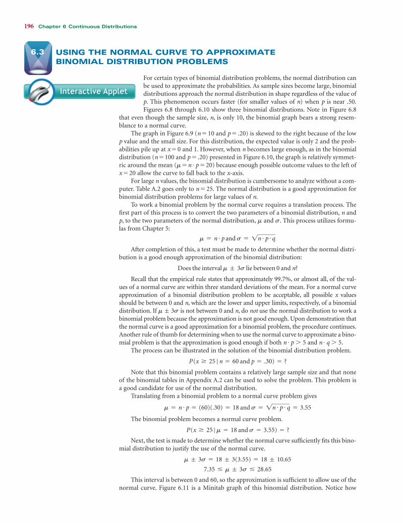
For certain types of binomial distribution problems, the normal distribution canbe used to approximate the probabilities. As sample sizes become large, binomialdistributions approach the normal distribution in shape regardless of the value ofp. This phenomenon occurs faster (for smaller values of n) when p is near .50.Figures 6.8 through 6.10 show three binomial distributions. Note in Figure 6.8

that even though the sample size, n, is only 10, the binomial graph bears a strong resem-blance to a normal curve.

The graph in Figure 6.9 (n = 10 and p = .20) is skewed to the right because of the lowp value and the small size. For this distribution, the expected value is only 2 and the prob-abilities pile up at x = 0 and 1. However, when n becomes large enough, as in the binomialdistribution (n = 100 and p = .20) presented in Figure 6.10, the graph is relatively symmet-ric around the mean ( = n p = 20) because enough possible outcome values to the left ofx = 20 allow the curve to fall back to the x-axis.

For large n values, the binomial distribution is cumbersome to analyze without a com-puter. Table A.2 goes only to n = 25. The normal distribution is a good approximation forbinomial distribution problems for large values of n.

To work a binomial problem by the normal curve requires a translation process. Thefirst part of this process is to convert the two parameters of a binomial distribution, n andp, to the two parameters of the normal distribution, and . This process utilizes formu-las from Chapter 5:

After completion of this, a test must be made to determine whether the normal distri-bution is a good enough approximation of the binomial distribution:

Recall that the empirical rule states that approximately 99.7%, or almost all, of the val-ues of a normal curve are within three standard deviations of the mean. For a normal curveapproximation of a binomial distribution problem to be acceptable, all possible x valuesshould be between 0 and n, which are the lower and upper limits, respectively, of a binomialdistribution. If 3 is not between 0 and n, do not use the normal distribution to work abinomial problem because the approximation is not good enough. Upon demonstration thatthe normal curve is a good approximation for a binomial problem, the procedure continues.Another rule of thumb for determining when to use the normal curve to approximate a bino-mial problem is that the approximation is good enough if both n p 5 and n q 5.

The process can be illustrated in the solution of the binomial distribution problem.

Note that this binomial problem contains a relatively large sample size and that noneof the binomial tables in Appendix A.2 can be used to solve the problem. This problem isa good candidate for use of the normal distribution.

Translating from a binomial problem to a normal curve problem gives

The binomial problem becomes a normal curve problem.

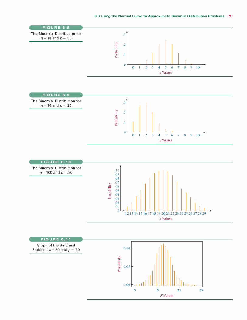
Next, the test is made to determine whether the normal curve sufficiently fits this bino-mial distribution to justify the use of the normal curve.

This interval is between 0 and 60, so the approximation is sufficient to allow use of thenormal curve. Figure 6.11 is a Minitab graph of this binomial distribution. Notice how

7.35 … m ; 3s … 28.65

m ; 3s = 18 ; 3(3.55) = 18 ; 10.65

P (x Ú 25 ƒ m = 18 and s = 3.55) = ?

m = n # p = (60)(.30) = 18 and s = 1n # p # q = 3.55

P (x Ú 25 ƒ n = 60 and p = .30) = ?

7#

7#

s;m

Does the interval m ; 3s lie between 0 and n?

m = n # p and s = 1n # p # q

sm

#m

USING THE NORMAL CURVE TO APPROXIMATE

BINOMIAL DISTRIBUTION PROBLEMS

6.3

JWCL152_C06_178-215.qxd 7/23/09 7:32 AM 6

6.3 Using the Normal Curve to Approximate Binomial Distribution Problems 197

0

Pro

babi

lity

x Values

0 1 2 3 4 5 6 7 8 9 10

.1

.2

.3The Binomial Distribution for

n = 10 and p = .50

FIGURE 6.8

0

Pro

babi

lity

x Values

0 1 2 3 4 5 6 7 8 9 10

.1

.2


n = 10 and p = .20

FIGURE 6.9

0

Pro

babi

lity

x Values

12 13 14 15 16 17 18 19 20 21 22 23 24 25 26 27 28 29

.01

.02

.03

.04

.05

.06

.07

.08

.09


n = 100 and p = .20

FIGURE 6.10

5 15

X Values

25 35

0.10

0.05

0.00

Pro

babi

lity

Graph of the Binomial

Problem: n = 60 and p = .30

FIGURE 6.11

JWCL152_C06_178-215.qxd 7/23/09 7:32 AM Page 197


closely it resembles the normal curve. Figure 6.12 is the apparent graph of the normal curveversion of this problem.

Correcting for Continuity

The translation of a discrete distribution to a continuous distribution is not completelystraightforward. A correction of +.50 or -.50 or .50, depending on the problem, isrequired. This correction ensures that most of the binomial problem’s information is cor-rectly transferred to the normal curve analysis. This correction is called the correction for continuity, which is made during conversion of a discrete distribution into a continuousdistribution.

Figure 6.13 is a portion of the graph of the binomial distribution, n = 60 and p = .30.Note that with a binomial distribution, all the probabilities are concentrated on the wholenumbers. Thus, the answers for x 25 are found by summing the probabilities for x = 25,26, 27, . . . , 60. There are no values between 24 and 25, 25 and 26, . . . , 59, and 60. Yet, thenormal distribution is continuous, and values are present all along the x-axis. A correctionmust be made for this discrepancy for the approximation to be as accurate as possible.

As an analogy, visualize the process of melting iron rods in a furnace. The iron rods arelike the probability values on each whole number of a binomial distribution. Note that thebinomial graph in Figure 6.13 looks like a series of iron rods in a line. When the rods areplaced in a furnace, they melt down and spread out. Each rod melts and moves to fill thearea between it and the adjacent rods. The result is a continuous sheet of solid iron (con-tinuous iron) that looks like the normal curve. The melting of the rods is analogous tospreading the binomial distribution to approximate the normal distribution.

How far does each rod spread toward the others? A good estimate is that each rod goesabout halfway toward the adjacent rods. In other words, a rod that was concentrated atx = 25 spreads to cover the area from 24.5 to 25.5; x = 26 becomes continuous from 25.5 to26.5; and so on. For the problem P (x 25 n = 60 and p = .30), conversion to a continu-ous normal curve problem yields P (x 24.5 = 18 and = 3.55). The correction forcontinuity was -.50 because the problem called for the inclusion of the value of 25 alongwith all greater values; the binomial value of x = 25 translates to the normal curve value of24.5 to 25.5. Had the binomial problem been to analyze P (x 25), the correction wouldhave been +.50, resulting in a normal curve problem of P (x 25.5). The latter case wouldbegin at more than 25 because the value of 25 would not be included.

The decision as to how to correct for continuity depends on the equality sign and thedirection of the desired outcomes of the binomial distribution. Table 6.4 lists some rules ofthumb that can help in the application of the correction for continuity.

For the binomial problem P (x 25 n = 60 and p = .30), the normal curve becomesP (x 24.5 = 18 and = 3.55), as shown in Figure 6.14, and

z =

x - m

s=

24.5 - 18

3.55= 1.83

smƒÚ

ƒÚ

Ú

7

smƒÚ

ƒÚ

Ú

;

= 18μ x ≥ 25 = 3.55σ

Graph of Apparent Solution of

Binomial Problem Worked by

the Normal Curve

FIGURE 6.12

0

Pro

babi

lity

x Values

13 26

.01

.02

.03

.04

.05

.06

.07

.08

.09

.10

.11

.12

14 15 16 17 18 19 20 21 22 23 24 25

Graph of a Portion of the

Binomial Problem: n = 60

and p = .30

FIGURE 6.13

Values Being Determined Corrections

x +.50

x -.50

x -.50

x +.50

x -.50 and +.50

x +.50 and -.50

x = -.50 and +.50

66

……

…

6

Ú

7

TABLE 6.4

Rules of Thumb for the

Correction for Continuity

JWCL152_C06_178-215.qxd 7/23/09 7:32 AM Page 198

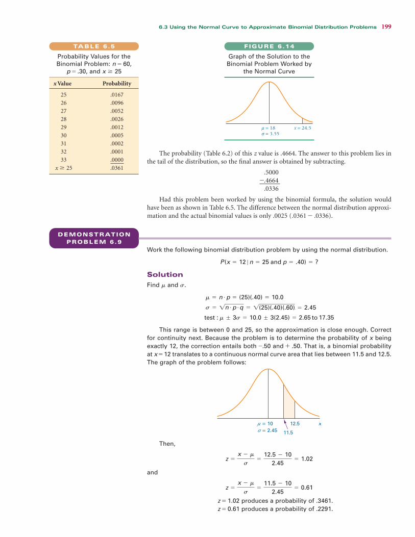
6.3 Using the Normal Curve to Approximate Binomial Distribution Problems 199

The probability (Table 6.2) of this z value is .4664. The answer to this problem lies inthe tail of the distribution, so the final answer is obtained by subtracting.

.5000-.4664

.0336

Had this problem been worked by using the binomial formula, the solution wouldhave been as shown in Table 6.5. The difference between the normal distribution approxi-mation and the actual binomial values is only .0025 (.0361 - .0336).

= 18μ x = 24.5 = 3.55σ

Graph of the Solution to the

Binomial Problem Worked by

the Normal Curve

FIGURE 6.14

x Value Probability

25 .0167

26 .0096

27 .0052

28 .0026

29 .0012

30 .0005

31 .0002

32 .0001

33 .0000

x 25 .0361Ú

TABLE 6.5

Probability Values for the

Binomial Problem: n = 60,

p = .30, and x 25Ú

DEMONSTRATION

PROBLEM 6.9

Work the following binomial distribution problem by using the normal distribution.

Solution

Find and .

This range is between 0 and 25, so the approximation is close enough. Correct

for continuity next. Because the problem is to determine the probability of x being

exactly 12, the correction entails both -.50 and + .50. That is, a binomial probability

at x = 12 translates to a continuous normal curve area that lies between 11.5 and 12.5.

The graph of the problem follows:

Then,

and

z = 1.02 produces a probability of .3461.

z = 0.61 produces a probability of .2291.

z =

x - m

s=

11.5 - 10

2.45= 0.61

z =

x - m

s=

12.5 - 10

2.45= 1.02

= 10μ 12.5 = 2.45σ

x

11.5

test : m ; 3s = 10.0 ; 3(2.45) = 2.65 to 17.35

s = 1n # p # q = 1(25)(.40)(.60) = 2.45

m = n # p = (25)(.40) = 10.0

sm

P (x = 12 ƒ n = 25 and p = .40) = ?

JWCL152_C06_178-215.qxd 7/23/09 7:32 AM Page 199


The difference in areas yields the following answer:

Had this problem been worked by using the binomial tables, the resulting answer

would have been .114. The difference between the normal curve approximation and

the value obtained by using binomial tables is only .003.

.3461 - .2291 = .1170

DEMONSTRATION

PROBLEM 6.10

Solve the following binomial distribution problem by using the normal distribution.

Solution

Because neither the sample size nor the p value is contained in Table A.2, working

this problem by using binomial distribution techniques is impractical. It is a good

candidate for the normal curve. Calculating and yields

Testing to determine the closeness of the approximation gives

The range 22.51 to 51.49 is between 0 and 100. This problem satisfies the conditions

of the test. Next, correct for continuity: x 27 as a binomial problem translates to

x 26.5 as a normal distribution problem. The graph of the problem follows.

Then,

Table 6.2 shows a probability of .4850. Solving for the tail of the distribution gives

which is the answer.

Had this problem been solved by using the binomial formula, the probabilities

would have been the following.

x Value Probability

26 .0059

25 .0035

24 .0019

23 .0010

22 .0005

21 .0002

20 .0001

x 27 .01316

.5000 - .4850 = .0150

z =

x - m

s=

26.5 - 37

4.83= -2.17

= 37μ = 4.83σ

x ≤ 26.5

…

6

m ; 3s = 37 ; 3(4.83) = 37 ; 14.49

s = 1n # p # q = 1(100)(.37)(.63) = 4.83

m = n # p = (100)(.37) = 37.0

sm

P (x 6 27 ƒ n = 100 and p = .37) = ?

JWCL152_C06_178-215.qxd 9/4/09 5:11 PM Page 200

Problems 201

The answer obtained by using the normal curve approximation (.0150) compares

favorably to this exact binomial answer. The difference is only .0019.

STATISTICS IN BUSINESS TODAY

Teleworking FactsThere are many interesting statistics about teleworkers. In arecent year, there were 45 million teleworkers in the UnitedStates, and more than 18% of employed adult Americanstelework from home during business hours at least one dayper month. Fifty-seven percent of HR professionals indicatethat their organizations offer some form of telecommuting.The typical teleworker works an average of 5.5 days at homeper month. The average commuting distance of a teleworkerwhen he/she is not teleworking is 18 miles. Teleworkers savean average of 53 minutes commuting each day, saving themthe equivalent of one extra day of work for every nine daysof commuting. Thirty-three percent of Canadians would

prefer to telework over a 10% wage increase, and 43% wouldchange jobs to an employer allowing telework. Sixty-fivepercent of home teleworkers are males versus 44% of non-teleworkers. Among 20 United States, government agencies,the average per-user cost of setting up telecommuting is$1,920. Telecommuting saves 840 million gallons of fuelannually in the United States, and telecommuting saves theequivalent of 9 to 14 billion kilowatt-hours of electricity peryear—the same amount of energy used by roughly 1 millionUnited States households every year.

Source: Telecommuting and Remote Work Statistics site at: http://www.suitecommute.com/Statistics.htm; and Telework Facts at: http://www.telcoa.org/id33_m.htm

6.3 PROBLEMS 6.17 Convert the following binomial distribution problems to normal distributionproblems. Use the correction for continuity.

a.

b.

c.

d.

6.18 Use the test 3 to determine whether the following binomial distributions canbe approximated by using the normal distribution.

a.

b.

c.

d.

e.

6.19 Where appropriate, work the following binomial distribution problems by using thenormal curve. Also, use Table A.2 to find the answers by using the binomial distribu-tion and compare the answers obtained by the two methods.

a.

b.

c.

d.

6.20 The Zimmerman Agency conducted a study for Residence Inn by Marriott of businesstravelers who take trips of five nights or more. According to this study, 37% of thesetravelers enjoy sightseeing more than any other activity that they do not get to do asmuch at home. Suppose 120 randomly selected business travelers who take trips offive nights or more are contacted. What is the probability that fewer than 40 enjoysightseeing more than any other activity that they do not get to do as much at home?

6.21 One study on managers’ satisfaction with management tools reveals that 59% of allmanagers use self-directed work teams as a management tool. Suppose 70 managersselected randomly in the United States are interviewed. What is the probability thatfewer than 35 use self-directed work teams as a management tool?

P (x 6 3 ƒ n = 10 and p = .70) = ?

P (x = 7 ƒ n = 15 and p = .50) = ?

P (x Ú 13 ƒ n = 20 and p = .60) = ?

P (x = 8 ƒ n = 25 and p = .40) = ?

n = 14 and p = .50

n = 30 and p = .75

n = 12 and p = .30

n = 18 and p = .80

n = 8 and p = .50

s;m

P (x 7 14 ƒ n = 16 and p = .45)

P (x = 22 ƒ n = 40 and p = .60)

P (10 6 x … 20) ƒ n = 25 and p = .50)

P (x … 16 ƒ n = 30 and p = .70)

JWCL152_C06_178-215.qxd 9/17/09 2:09 PM Page 201

http://www.suitecommute.com/Statistics.htm

http://www.telcoa.org/id33_m.htm


6.22 According to the Yankee Group, 53% of all cable households rate cable companies asgood or excellent in quality transmission. Sixty percent of all cable households ratecable companies as good or excellent in having professional personnel. Suppose 300 cable households are randomly contacted.

a. What is the probability that more than 175 cable households rate cable companies as good or excellent in quality transmission?

b. What is the probability that between 165 and 170 (inclusive) cable householdsrate cable companies as good or excellent in quality transmission?

c. What is the probability that between 155 and 170 (inclusive) cable householdsrate cable companies as good or excellent in having professional personnel?

d. What is the probability that fewer than 200 cable households rate cable companies as good or excellent in having professional personnel?

6.23 Market researcher Gartner Dataquest reports that Dell Computer controls 27% ofthe PC market in the United States. Suppose a business researcher randomly selects130 recent purchasers of PC.

a. What is the probability that more than 39 PC purchasers bought a Dell computer?

b. What is the probability that between 28 and 38 PC purchasers (inclusive) boughta Dell computer?

c. What is the probability that fewer than 23 PC purchasers bought a Dell computer?

d. What is the probability that exactly 33 PC purchasers bought a Dell computer?

6.24 A study about strategies for competing in the global marketplace states that 52%of the respondents agreed that companies need to make direct investments in foreign countries. It also states that about 70% of those responding agree that it is attractive to have a joint venture to increase global competitiveness. SupposeCEOs of 95 manufacturing companies are randomly contacted about globalstrategies.

a. What is the probability that between 44 and 52 (inclusive) CEOs agree that compa-nies should make direct investments in foreign countries?

b. What is the probability that more than 56 CEOs agree with that assertion?

c. What is the probability that fewer than 60 CEOs agree that it is attractive to havea joint venture to increase global competitiveness?

d. What is the probability that between 55 and 62 (inclusive) CEOs agree with thatassertion?

Another useful continuous distribution is the exponential distribution. It is closely relatedto the Poisson distribution. Whereas the Poisson distribution is discrete and describesrandom occurrences over some interval, the exponential distribution is continuous anddescribes a probability distribution of the times between random occurrences. The followingare the characteristics of the exponential distribution.

■ It is a continuous distribution.

■ It is a family of distributions.

■ It is skewed to the right.

■ The x values range from zero to infinity.

■ Its apex is always at x = 0.

■ The curve steadily decreases as x gets larger.

The exponential probability distribution is determined by the following.

EXPONENTIAL DISTRIBUTION6.4

JWCL152_C06_178-215.qxd 7/23/09 7:32 AM Page 202

6.4 Exponential Distribution 203

An exponential distribution can be characterized by the one parameter, . Eachunique value of determines a different exponential distribution, resulting in a family ofexponential distributions. Figure 6.15 shows graphs of exponential distributions for fourvalues of . The points on the graph are determined by using and various values of x inthe probability density formula. The mean of an exponential distribution is = 1 , andthe standard deviation of an exponential distribution is = 1 .

Probabilities of the Exponential Distribution

Probabilities are computed for the exponential distribution by determining the area underthe curve between two points. Applying calculus to the exponential probability densityfunction produces a formula that can be used to calculate the probabilities of an exponen-tial distribution.

l>s

l>m

ll

l

l

EXPONENTIALPROBABILITY DENSITYFUNCTION

wherex 0

0and e = 2.71828 . . .

7l

Ú

f (x) = le-lx

PROBABILITIES OF THE RIGHT TAIL OF THE EXPONENTIALDISTRIBUTION

where:x0 Ú 0

P (x Ú x0) = e-lx0

0 1 2

f(x)

x

λ

= .5

= 2.0λ

= .2

= 1.0λ

λ

.2

.5

1.0

2.0

3 4 5 6 7

Graphs of Some Exponential

Distributions

FIGURE 6.15

To use this formula requires finding values of e-x. These values can be computed onmost calculators or obtained from Table A.4, which contains the values of e-x for selectedvalues of x. x0 is the fraction of the interval or the number of intervals between arrivals inthe probability question and is the average arrival rate.

For example, arrivals at a bank are Poisson distributed with a of 1.2 customers everyminute. What is the average time between arrivals and what is the probability that at least2 minutes will elapse between one arrival and the next arrival? Since the interval for lambdais 1 minute and we want to know the probability that at least 2 minutes transpire betweenarrivals (twice the lambda interval), x0 is 2.

Interarrival times of random arrivals are exponentially distributed. The mean of thisexponential distribution is = 1 = 1 1.2 =.833 minute (50 seconds). On average,>l>m

l

l

JWCL152_C06_178-215.qxd 7/23/09 7:32 AM Page 203


.833 minute, or 50 seconds, will elapse between arrivals at the bank. The probability of aninterval of 2 minutes or more between arrivals can be calculated by

About 9.07% of the time when the rate of random arrivals is 1.2 per minute, 2 min-utes or more will elapse between arrivals, as shown in Figure 6.16.

This problem underscores the potential of using the exponential distribution in con-junction with the Poisson distribution to solve problems. In operations research and man-agement science, these two distributions are used together to solve queuing problems (theoryof waiting lines). The Poisson distribution can be used to analyze the arrivals to the queue,and the exponential distribution can be used to analyze the interarrival time.

P (x Ú 2 ƒ l = 1.2) = e-1.2(2)= .0907.

0

f(x)

x.1.2.3.4.5.6.7.8.9

1.01.11.2

1 2 3

Exponential Distribution for

= 1.2 and Solution for x 2Úl

FIGURE 6.16

DEMONSTRATION

PROBLEM 6.11

A manufacturing firm has been involved in statistical quality control for several years.

As part of the production process, parts are randomly selected and tested. From the

records of these tests, it has been established that a defective part occurs in a pattern

that is Poisson distributed on the average of 1.38 defects every 20 minutes during

production runs. Use this information to determine the probability that less than

15 minutes will elapse between any two defects.

Solution

The value of is 1.38 defects per 20-minute interval. The value of can be determined by

On the average, it is .7246 of the interval, or (.7246)(20 minutes) = 14.49 minutes,

between defects. The value of x0 represents the desired number of intervals between

arrivals or occurrences for the probability question. In this problem, the probability

question involves 15 minutes and the interval is 20 minutes. Thus x0 is 15 20, or .75

of an interval. The question here is to determine the probability of there being less

than 15 minutes between defects. The probability formula always yields the right tail

of the distribution—in this case, the probability of there being 15 minutes or more

between arrivals. By using the value of x0 and the value of , the probability of there

being 15 minutes or more between defects can be determined.

The probability of .3552 is the probability that at least 15 minutes will elapse between

defects. To determine the probability of there being less than 15 minutes between

defects, compute 1 - P(x). In this case, 1 - .3552 = .6448. There is a probability of .6448 that

less than 15 minutes will elapse between two defects when there is an average of 1.38

defects per 20-minute interval or an average of 14.49 minutes between defects.

P (x Ú x0) = P (x Ú .75) = e-lx0= e(-1.38)(.75)

= e-1.035= .3552

l

>

m =

1

l=

1

1.38= .7246

ml

JWCL152_C06_178-215.qxd 7/23/09 7:32 AM Page 204

Problems 205

Using the Computer to Determine ExponentialDistribution Probabilities

Both Excel and Minitab can be used to solve for exponential distribution probabilities.Excel uses the value of and x0, but Minitab requires (equals 1 ) and x0. In each case,the computer yields the cumulative probability from the left (the complement of what theprobability formula shown in this section yields). Table 6.6 provides Excel and Minitaboutput for the probability question addressed in Demonstration Problem 6.11.

l>ml

Excel and Minitab Output for

Exponential Distribution

Minitab Output


Exponential with mean = 0.7246

x P(X <= x)

0.75 0.644793

Excel Output

x Value Probability < x Value

0.75 0.6448

6.4 PROBLEMS 6.25 Use the probability density formula to sketch the graphs of the following exponentialdistributions.

a. = 0.1

b. = 0.3

c. = 0.8

d. = 3.0

6.26 Determine the mean and standard deviation of the following exponential distributions.

a. = 3.25

b. = 0.7

c. = 1.1

d. = 6.0

6.27 Determine the following exponential probabilities.

a. P (x 5 = 1.35)

b. P (x 3 = 0.68)

c. P (x 4 = 1.7)

d. P (x 6 = 0.80)

6.28 The average length of time between arrivals at a turnpike tollbooth is 23 seconds.Assume that the time between arrivals at the tollbooth is exponentially distributed.

a. What is the probability that a minute or more will elapse between arrivals?

b. If a car has just passed through the tollbooth, what is the probability that no carwill show up for at least 3 minutes?

6.29 A busy restaurant determined that between 6:30 P.M. and 9:00 P.M. on Friday nights,the arrivals of customers are Poisson distributed with an average arrival rate of 2.44per minute.

a. What is the probability that at least 10 minutes will elapse between arrivals?

b. What is the probability that at least 5 minutes will elapse between arrivals?

c. What is the probability that at least 1 minute will elapse between arrivals?

d. What is the expected amount of time between arrivals?

lƒ6

lƒ7

lƒ6

lƒÚ

l

l

l

l

l

l

l

l

TABLE 6.6

JWCL152_C06_178-215.qxd 7/23/09 7:32 AM Page 205


6.30 During the summer at a small private airport in western Nebraska, the unscheduledarrival of airplanes is Poisson distributed with an average arrival rate of 1.12 planesper hour.

a. What is the average interarrival time between planes?

b. What is the probability that at least 2 hours will elapse between plane arrivals?

c. What is the probability of two planes arriving less than 10 minutes apart?

6.31 The exponential distribution can be used to solve Poisson-type problems in whichthe intervals are not time. The Airline Quality Rating Study published by the U.S.Department of Transportation reported that in a recent year, Airtran led the nationin fewest occurrences of mishandled baggage, with a mean rate of 4.06 per 1,000passengers. Assume mishandled baggage occurrences are Poisson distributed. Usingthe exponential distribution to analyze this problem, determine the average numberof passengers between occurrences. Suppose baggage has just been mishandled.

a. What is the probability that at least 500 passengers will have their baggagehandled properly before the next mishandling occurs?

b. What is the probability that the number will be fewer than 200 passengers?

6.32 The Foundation Corporation specializes in constructing the concrete foundationsfor new houses in the South. The company knows that because of soil types, mois-ture conditions, variable construction, and other factors, eventually most founda-tions will need major repair. On the basis of its records, the company’s presidentbelieves that a new house foundation on average will not need major repair for20 years. If she wants to guarantee the company’s work against major repair but wantsto have to honor no more than 10% of its guarantees, for how many years shouldthe company guarantee its work? Assume that occurrences of major foundationrepairs are Poisson distributed.

6.33 During the dry month of August, one U.S. city has measurable rain on averageonly two days per month. If the arrival of rainy days is Poisson distributed inthis city during the month of August, what is the average number of days thatwill pass between measurable rain? What is the standard deviation? What is theprobability during this month that there will be a period of less than two daysbetween rain?

The American Society for Trainingand Development reported that,on average, an employee receives

32 hours of training per year. Suppose that number of hours oftraining is uniformly distributed across all employees varyingfrom 0 hours to 64 hours. Using techniques presented inSection 6.1, this uniform distribution can be described by a = 0, b = 64, and = 32. The probability that an employeereceives between 20 and 40 hours of training can be determinedby the following calculation assuming that x1 = 20 and x2 = 40:

P (x) =

x2 - x1

b - a=

40 - 20

64 - 0=

20

64= .3125

m

Thus, 31.25% of employees receive between 20 and 40 hoursof training.

The probability that an employee receives 50 hours ormore of training can be calculated as:

Almost 22% of employees receive 50 hours or more of train-ing. Note that here, x2 is 64 since 64 hours is the upper end ofthe distribution.

It is estimated by some studies that, on average, it costs$3,270 to hire an employee. If such costs are normally distrib-uted with a standard deviation of $400, the probability that itcosts more than $4,000 to hire an employee can be calculatedusing techniques from Section 6.2 as:

z =

x - m

s=

4000 - 3270

400= 1.83

P (x) =

x2 - x1

b - a=

64 - 50

64 - 0=

14

64= .21875

The Cost of Human Resources

JWCL152_C06_178-215.qxd 7/23/09 7:32 AM Page 206

Summary 207

The area associated with this z value is .4664 and the tailof the distribution is .5000 - .4664 = .0336. That is, 3.36% ofthe time, it costs more than $4,000 to hire an employee. Theprobability that it costs less than $3,000 to hire an employeecan be determined in a similar manner:

The area associated with this z value is .2517 and the tail of thedistribution is .5000 - .2517 = .2483. That is, 24.83% of thetime, it costs less than $3,000 to hire an employee.

Thirty-five percent of all unscheduled absenteeism iscaused by personal illness. Using techniques presented inSection 6.3, the probability that more than 50 of 120 ran-domly selected unscheduled absences were caused by personalillness can be determined. With n = 120, p = .35 and x 50,this binomial distribution problem can be converted into a

7

z =

x - m

s=

3000 - 3270

400= 0.68

normal distribution problem by:

and

Since 42 3(5.225) is between 0 and 120, it is appropriate touse the normal distribution to approximate this binomialproblem. Applying the correction for continuity, x 50.5.The z value is calculated as:

The area associated with this z value is .4484 and the tail of thedistribution is .5000 - .4484 = .0516. That is, 5.16% of thetime, more than 50 out of 120 unscheduled absences are due topersonal illness.

z =

x - m

s=

50.5 - 42

5.225= 1.63

Ú

;

s = 1n # p # q = 1(120)(.35)(.65) = 5.225

m = n # p = (120)(.35) = 42

Several points must be considered in working with con-tinuous distributions. Is the population being studied thesame population from which the parameters (mean, stan-dard deviation, ) were determined? If not, the resultsmay not be valid for the analysis being done. Invalid orspurious results can be obtained by using the parametersfrom one population to analyze another population. Forexample, a market study in New England may result in theconclusion that the amount of fish eaten per month by adults is normally distributed with the average of2.3 pounds of fish per month. A market researcher in theSouthwest should not assume that these figures apply toher population. People in the Southwest probably havequite different fish-eating habits than people in NewEngland, and the application of New England populationparameters to the Southwest probably will result in ques-tionable conclusions.

As was true with the Poisson distribution in Chapter 5,the use of in the exponential distribution should bejudicious because a for one interval in a given time

period or situation may not be the same as the for thesame interval in a different time period or situation. Forexample, the number of arrivals per five-minute timeperiod at a restaurant on Friday night is not likely to bethe same as the number of arrivals in a five-minute timeperiod at that same restaurant from 2 P.M. to 4 P.M. onweekdays. In using established parameters such as and

, a researcher should be certain that the population fromwhich the parameter was determined is, indeed, the samepopulation being studied.

Sometimes a normal distribution is used to analyze datawhen, in fact, the data are not normal. Such an analysis cancontain bias and produce false results. Certain techniquesfor testing a distribution of data can determine whetherthey are distributed a certain way. Some of the techniquesare presented in Chapter 16. In general, Chapter 6 tech-niques can be misused if the wrong type of distribution isapplied to the data or if the distribution used for analysis isthe right one but the parameters ( , , ) do not fit thedata of the population being analyzed. ›

lsm

l

m

l

l

l

l

ETHICAL CONSIDERATIONS

SUMMARY

This chapter discussed three different continuous distributions:the uniform distribution, the normal distribution, and the expo-nential distribution. With continuous distributions, the valueof the probability density function does not yield the proba-bility but instead gives the height of the curve at any givenpoint. In fact, with continuous distributions, the probability atany discrete point is .0000. Probabilities are determined overan interval. In each case, the probability is the area under the

curve for the interval being considered. In each distribution,the probability or total area under the curve is 1.

Probably the simplest of these distributions is the uni-form distribution, sometimes referred to as the rectangulardistribution. The uniform distribution is determined from aprobability density function that contains equal values alongsome interval between the points a and b. Basically, theheight of the curve is the same everywhere between these

JWCL152_C06_178-215.qxd 7/23/09 7:32 AM Page 207


two points. Probabilities are determined by calculating theportion of the rectangle between the two points a and b thatis being considered.

The most widely used of all distributions is the normal dis-tribution. Many phenomena are normally distributed, includ-ing characteristics of most machine-produced parts, manymeasurements of the biological and natural environment, andmany human characteristics such as height, weight, IQ, andachievement test scores. The normal curve is continuous,symmetrical, unimodal, and asymptotic to the axis; actually, itis a family of curves.

The parameters necessary to describe a normal distribu-tion are the mean and the standard deviation. For conven-ience, data that are being analyzed by the normal curve shouldbe standardized by using the mean and the standard deviationto compute z scores. A z score is the distance that an x value isfrom the mean, , in units of standard deviations. With the zscore of an x value, the probability of that value occurring bychance from a given normal distribution can be determinedby using a table of z scores and their associated probabilities.

m

The normal distribution can be used to work certain typesof binomial distribution problems. Doing so requires convert-ing the n and p values of the binomial distribution to andof the normal distribution. When worked by using the normaldistribution, the binomial distribution solution is only anapproximation. If the values of 3 are within a rangefrom 0 to n, the approximation is reasonably accurate.Adjusting for the fact that a discrete distribution problem isbeing worked by using a continuous distribution requires acorrection for continuity. The correction for continuityinvolves adding or subtracting .50 to the x value being ana-lyzed. This correction usually improves the normal curveapproximation.

Another continuous distribution is the exponential distri-bution. It complements the discrete Poisson distribution. Theexponential distribution is used to compute the probabilitiesof times between random occurrences. The exponential dis-tribution is a family of distributions described by one param-eter, . The distribution is skewed to the right and always hasits highest value at x = 0.l

s;m

sm

KEY TERMS

correction for continuityexponential distributionnormal distribution

rectangular distributionstandardized normal

distribution

uniform distributionz distributionz score

FORMULAS

Probability density function of a uniform distribution

Mean and standard deviation of a uniform distribution

Probability density function of the normal distribution

f (x) =

1

s12pe-(1>2)[(x -m)>s]2

s =

b - a

112

m =

a + b

2

f (x) = L1

b - afor a … x … b

0 for all other values

z formula

Conversion of a binomial problem to the normal curve

Exponential probability density function

Probabilities of the right tail of the exponential distribution

P (x Ú x0) = e-lx0

f (x) = le-lx

m = n # p and s = 1n # p # q

z =

x - m

s

SUPPLEMENTARY PROBLEMS

CALCULATING THE STATISTICS

6.34 Data are uniformly distributed between the values of 6and 14. Determine the value of f (x). What are the meanand standard deviation of this distribution? What is theprobability of randomly selecting a value greater than 11?What is the probability of randomly selecting a valuebetween 7 and 12?

6.35 Assume a normal distribution and find the followingprobabilities.

a. P (x 21 = 25 and = 4)b. P (x 77 = 50 and = 9)c. P (x 47 = 50 and = 6)d. P (13 x 29 = 23 and = 4)e. P (x 105 = 90 and = 2.86)smƒÚ

smƒ66

smƒ7

smƒÚ

smƒ6

JWCL152_C06_178-215.qxd 7/23/09 7:33 AM Page 208

Supplementary Problems 209

6.36 Work the following binomial distribution problems byusing the normal distribution. Check your answers byusing Table A.2 to solve for the probabilities.

a. P (x = 12 n = 25 and p = .60)

b. P (x 5 n = 15 and p = .50)

c. P (x 3 n = 10 and p = .50)

d. P (x 8 n = 15 and p = .40)

6.37 Find the probabilities for the following exponential dis-tribution problems.

a. P (x 3 = 1.3)

b. P (x 2 = 2.0)

c. P (1 x 3 = 1.65)

d. P (x 2 = .405)

TESTING YOUR UNDERSTANDING

6.38 The U.S. Bureau of Labor Statistics reports that of per-sons who usually work full-time, the average number ofhours worked per week is 43.4. Assume that the numberof hours worked per week for those who usually workfull-time is normally distributed. Suppose 12% of theseworkers work more than 48 hours. Based on this per-centage, what is the standard deviation of number ofhours worked per week for these workers?

6.39 A U.S. Bureau of Labor Statistics survey showed that onein five people 16 years of age or older volunteers some ofhis or her time. If this figure holds for the entire popula-tion and if a random sample of 150 people 16 years ofage or older is taken, what is the probability that morethan 50 of those sampled do volunteer work?

6.40 An entrepreneur opened a small hardware store in a stripmall. During the first few weeks, business was slow, withthe store averaging only one customer every 20 minutes inthe morning. Assume that the random arrival of customersis Poisson distributed.

a. What is the probability that at least one hour wouldelapse between customers?

b. What is the probability that 10 to 30 minutes wouldelapse between customers?

c. What is the probability that less than five minuteswould elapse between customers?

6.41 In a recent year, the average price of a Microsoft WindowsUpgrade was $90.28 according to PC Data. Assume thatprices of the Microsoft Windows Upgrade that year werenormally distributed, with a standard deviation of $8.53.If a retailer of computer software was randomly selectedthat year:

a. What is the probability that the price of a MicrosoftWindows Upgrade was below $80?

b. What is the probability that the price was above $95?

c. What is the probability that the price was between $83and $87?

6.42 According to the U.S. Department of Agriculture,Alabama egg farmers produce millions of eggs every

lƒ7

lƒ……

lƒ6

lƒÚ

ƒÚ

ƒ…

ƒ7

ƒ

year. Suppose egg production per year in Alabama isnormally distributed, with a standard deviation of83 million eggs. If during only 3% of the years Alabamaegg farmers produce more than 2,655 million eggs, whatis the mean egg production by Alabama farmers?

6.43 The U.S. Bureau of Labor Statistics releases figures onthe number of full-time wage and salary workers withflexible schedules. The numbers of full-time wage andsalary workers in each age category are almost uniformlydistributed by age, with ages ranging from 18 to 65 years.If a worker with a flexible schedule is randomly drawnfrom the U.S. workforce, what is the probability that heor she will be between 25 and 50 years of age? What isthe mean value for this distribution? What is the heightof the distribution?

6.44 A business convention holds its registration on Wednesdaymorning from 9:00 A.M. until 12:00 noon. Past historyhas shown that registrant arrivals follow a Poisson distri-bution at an average rate of 1.8 every 15 seconds. Fort-unately, several facilities are available to register conventionmembers.

a. What is the average number of seconds between arrivalsto the registration area for this conference based onpast results?

b. What is the probability that 25 seconds or more wouldpass between registration arrivals?

c. What is the probability that less than five seconds willelapse between arrivals?

d. Suppose the registration computers went down for aone-minute period. Would this condition pose aproblem? What is the probability that at least oneminute will elapse between arrivals?

6.45 M/PF Research, Inc. lists the average monthly apartmentrent in some of the most expensive apartment rentallocations in the United States. According to their report,the average cost of renting an apartment in Minneapolisis $951. Suppose that the standard deviation of the costof renting an apartment in Minneapolis is $96 and thatapartment rents in Minneapolis are normally distrib-uted. If a Minneapolis apartment is randomly selected,what is the probability that the price is:

a. $1,000 or more?

b. Between $900 and $1,100?

c. Between $825 and $925?

d. Less than $700?

6.46 According to The Wirthlin Report, 24% of all workers saythat their job is very stressful. If 60 workers are randomlyselected:

a. What is the probability that 17 or more say that theirjob is very stressful?

b. What is the probability that more than 22 say thattheir job is very stressful?

c. What is the probability that between 8 and 12 (inclu-sive) say that their job is very stressful?

JWCL152_C06_178-215.qxd 7/23/09 7:33 AM Page 209


6.47 The U.S. Bureau of Economic Statistics reports that theaverage annual salary in the metropolitan Boston area is$50,542. Suppose annual salaries in the metropolitanBoston area are normally distributed with a standard devi-ation of $4,246. A Boston worker is randomly selected.

a. What is the probability that the worker’s annual salaryis more than $60,000?

b. What is the probability that the worker’s annual salaryis less than $45,000?

c. What is the probability that the worker’s annual salaryis more than $40,000?

d. What is the probability that the worker’s annual salaryis between $44,000 and $52,000?

6.48 Suppose interarrival times at a hospital emergency roomduring a weekday are exponentially distributed, with anaverage interarrival time of nine minutes. If the arrivalsare Poisson distributed, what would the average numberof arrivals per hour be? What is the probability that lessthan five minutes will elapse between any two arrivals?

6.49 Suppose the average speeds of passenger trains travelingfrom Newark, New Jersey, to Philadelphia, Pennsylvania,are normally distributed, with a mean average speed of88 miles per hour and a standard deviation of 6.4 milesper hour.

a. What is the probability that a train will average lessthan 70 miles per hour?

b. What is the probability that a train will average morethan 80 miles per hour?

c. What is the probability that a train will average between90 and 100 miles per hour?

6.50 The Conference Board published information on whycompanies expect to increase the number of part-timejobs and reduce full-time positions. Eighty-one percent ofthe companies said the reason was to get a flexible work-force. Suppose 200 companies that expect to increase thenumber of part-time jobs and reduce full-time positionsare identified and contacted. What is the expected num-ber of these companies that would agree that the reason isto get a flexible workforce? What is the probability thatbetween 150 and 155 (not including the 150 or the 155)would give that reason? What is the probability that morethan 158 would give that reason? What is the probabilitythat fewer than 144 would give that reason?

6.51 According to the U.S. Bureau of the Census, about 75%of commuters in the United States drive to work alone.Suppose 150 U.S. commuters are randomly sampled.

a. What is the probability that fewer than 105 commutersdrive to work alone?

b. What is the probability that between 110 and 120(inclusive) commuters drive to work alone?

c. What is the probability that more than 95 commutersdrive to work alone?

6.52 According to figures released by the National AgriculturalStatistics Service of the U.S. Department of Agriculture,the U.S. production of wheat over the past 20 years hasbeen approximately uniformly distributed. Suppose themean production over this period was 2.165 billionbushels. If the height of this distribution is .862 billionbushels, what are the values of a and b for this distribution?

6.53 The Federal Reserve System publishes data on familyincome based on its Survey of Consumer Finances. Whenthe head of the household has a college degree, the meanbefore-tax family income is $85,200. Suppose that 60% ofthe before-tax family incomes when the head of the house-hold has a college degree are between $75,600 and $94,800and that these incomes are normally distributed. What isthe standard deviation of before-tax family incomes whenthe head of the household has a college degree?

6.54 According to the Polk Company, a survey of householdsusing the Internet in buying or leasing cars reported that81% were seeking information about prices. In addition,44% were seeking information about products offered.Suppose 75 randomly selected households who are usingthe Internet in buying or leasing cars are contacted.

a. What is the expected number of households who areseeking price information?

b. What is the expected number of households who areseeking information about products offered?

c. What is the probability that 67 or more householdsare seeking information about prices?

d. What is the probability that fewer than 23 householdsare seeking information about products offered?

6.55 Coastal businesses along the Gulf of Mexico from Texas toFlorida worry about the threat of hurricanes during theseason from June through October. Businesses becomeespecially nervous when hurricanes enter the Gulf ofMexico. Suppose the arrival of hurricanes during this sea-son is Poisson distributed, with an average of three hurri-canes entering the Gulf of Mexico during the five-monthseason. If a hurricane has just entered the Gulf of Mexico:

a. What is the probability that at least one month willpass before the next hurricane enters the Gulf?

b. What is the probability that another hurricane willenter the Gulf of Mexico in two weeks or less?

c. What is the average amount of time between hurri-canes entering the Gulf of Mexico?

6.56 With the growing emphasis on technology and thechanging business environment, many workers are dis-covering that training such as reeducation, skill develop-ment, and personal growth are of great assistance in thejob marketplace. A recent Gallup survey found that 80%of Generation Xers considered the availability ofcompany-sponsored training as a factor to weigh in tak-ing a job. If 50 Generation Xers are randomly sampled,what is the probability that fewer than 35 consider the

JWCL152_C06_178-215.qxd 7/23/09 7:33 AM Page 210

Supplementary Problems 211

availability of company-sponsored training as a factor toweigh in taking a job? What is the expected number?What is the probability that between 42 and 47 (inclusive)consider the availability of company-sponsored trainingas a factor to weigh in taking a job?

6.57 According to the Air Transport Association of America, theaverage operating cost of an MD-80 jet airliner is $2,087 perhour. Suppose the operating costs of an MD-80 jet airlinerare normally distributed with a standard deviation of $175per hour. At what operating cost would only 20% of theoperating costs be less? At what operating cost would 65%of the operating costs be more? What operating cost wouldbe more than 85% of operating costs?

6.58 Supermarkets usually become busy at about 5 P.M. onweekdays, because many workers stop by on the wayhome to shop. Suppose at that time arrivals at a super-market’s express checkout station are Poisson distrib-uted, with an average of .8 person/minute. If the clerkhas just checked out the last person in line, what is theprobability that at least one minute will elapse before thenext customer arrives? Suppose the clerk wants to go tothe manager’s office to ask a quick question and needs2.5 minutes to do so. What is the probability that theclerk will get back before the next customer arrives?

6.59 In a recent year, the average daily circulation of The WallStreet Journal was 1,717,000. Suppose the standard devi-ation is 50,940. Assume the paper’s daily circulation isnormally distributed. On what percentage of days wouldcirculation pass 1,800,000? Suppose the paper cannotsupport the fixed expenses of a full-production setup ifthe circulation drops below 1,600,000. If the probabilityof this even occurring is low, the production managermight try to keep the full crew in place and not disruptoperations. How often will this even happen, based onthis historical information?

6.60 Incoming phone calls generally are thought to be Poissondistributed. If an operator averages 2.2 phone calls every30 seconds, what is the expected (average) amount of timebetween calls? What is the probability that a minute ormore would elapse between incoming calls? Two minutes?

INTERPRETING THE OUTPUT

6.61 Shown here is a Minitab output. Suppose the data repre-sent the number of sales associates who are working in adepartment store in any given retail day. Describe thedistribution including the mean and standard deviation.Interpret the shape of the distribution and the mean inlight of the data being studied. What do the probabilitystatements mean?


Continuous uniform on 11 to 32

x P(X = x)28 0.80952

34 1.00000

16 0.23810

21 0.47619

6

6.63 Suppose the Minitab output shown here represents theanalysis of the length of home-use cell phone calls interms of minutes. Describe the distribution of cell phonecall lengths and interpret the meaning of the probabilitystatements.


Normal with mean = 2.35 and standard deviation = 0.11

x P(X = x)2.60 0.988479

2.45 0.818349

2.30 0.324718

2.00 0.000732

6.64 A restaurant averages 4.51 customers per 10 minutesduring the summer in the late afternoon. Shown here areExcel and Minitab output for this restaurant. Discuss the type of distribution used to analyze the data and themeaning of the probabilities.

6

Normal DistributionMean = 227 mg.Standard Deviation = 2.3 mg.

x Value Probability < x Value220 0.0012225 0.1923227 0.5000231 0.9590238 1.0000

x Value0.1 0.36300.2 0.59420.5 0.89511.0 0.98902.4 1.0000

Probability < x Value

Exponential Distribution


Exponential with mean = 0.221729

x P(X = x)0.1 0.363010

0.2 0.594243

0.5 0.895127

1.0 0.989002

2.4 0.999980

6

6.62 A manufacturing company produces a metal rod. Usethe Excel output shown here to describe the weight ofthe rod. Interpret the probability values in terms of themanufacturing process.

JWCL152_C06_178-215.qxd 7/23/09 7:33 AM Page 211


ANALYZING THE DATABASES

1. The Consumer Food database contains a variable, AnnualFood Spending, which represents the amount spent perhousehold on food for a year. Calculate the mean and stan-dard deviation for this variable that is approximately normallydistributed in this database. Using the mean and standarddeviation, calculate the probability that a randomly selectedhousehold spends more than $10,000 annually on food.What is the probability that a randomly selected householdspends less than $5,000 annually on food? What is the prob-ability that a randomly selected household spends between$8,000 and $11,000 annually on food?

2. Select the Agribusiness time-series database. Create a his-togram graph for onions and for broccoli. Each of thesevariables is approximately normally distributed. Com-pute the mean and the standard deviation for each distri-bution. The data in this database represent the monthlyweight (in thousands of pounds) of each vegetable. Interms of monthly weight, describe each vegetable (onionsand broccoli). If a month were randomly selected from

the onion distribution, what is the probability that theweight would be more than 50,000? What is the probabilitythat the weight would be between 25,000 and 35,000? If amonth were randomly selected from the broccoli distri-bution, what is the probability that the weight would bemore than 100,000? What is the probability that theweight would be between 135,000 and 170,000?

3. From the Hospital database, it can be determined thatsome hospitals admit around 50 patients per day. Supposewe select a hospital that admits 50 patients per day.Assuming that admittance only occurs within a 12-hourtime period each day and that admittance is Poisson dis-tributed, what is the value of lambda for per hour for thishospital? What is the interarrival time for admittance basedon this figure? Suppose a person was just admitted to thehospital. What the probability that it would be more than30 minutes before the next person was admitted? What isthe probability that there would be less than 10 minutesbefore the next person was admitted?

see www.wiley.com/college/black

CASE

Mercedes and BMW have been competing head-to-head formarket share in the luxury-car market for more than fourdecades. Back in 1959, BMW (Bayerische Motoren Werke)almost went bankrupt and nearly sold out to Daimler-Benz,the maker of Mercedes-Benz cars. BMW was able to recover tothe point that in 1992 it passed Mercedes in worldwide sales.Among the reasons for BMW’s success was its ability to sellmodels that were more luxurious than previous models butstill focused on consumer quality and environmental respon-sibility. In particular, BMW targeted its sales pitch to theyounger market, whereas Mercedes retained a more maturecustomer base.

In response to BMW’s success, Mercedes has been trying tochange their image by launching several products in an effortto attract younger buyers who are interested in sporty,performance-oriented cars. BMW, influenced by Mercedes, ispushing for more refinement and comfort. In fact, one auto-motive expert says that Mercedes wants to become BMW, andvice versa. However, according to one recent automotiveexpert, the focus is still on luxury and comfort for Mercedeswhile BMW focuses on performance and driving dynamics.Even though each company produces many different models,two relatively comparable coupe automobiles are the BMW 3Series Coupe 335i and the Mercedes CLK350 Coupe. In arecent year, the national U.S. market price for the BMW 3Series Coupe 335i was $39,368 and for the Mercedes CLK350Couple was $44,520. Gas mileage for both of these cars isaround 17 mpg in town and 25 mpg on the highway.

Discussion

1. Suppose Mercedes is concerned that dealer prices of theCLK350 Coupe are not consistent and that even thoughthe average price is $44,520, actual prices are normallydistributed with a standard deviation of $2,981. Supposealso that Mercedes believes that at $43,000, the CLK350Coupe is priced out of the BMW 3 Series Coupe 335imarket. What percentage of the dealer prices for theMercedes CLK350 Coupe is more than $43,000 and hencepriced out of the BMW 3 Series Coupe 335i market? Theaverage price for a BMW 3 Series Coupe 335i is $39,368.Suppose these prices are also normally distributed with astandard deviation of $2,367. What percentage of BMWdealers are pricing the BMW 3 Series Coupe 335i at morethan the average price for a Mercedes CLK350 Coupe?What might this mean to BMW if dealers were pricing the3 Series Couple 351 at this level? What percentage ofMercedes dealers are pricing the CLK350 Couple at lessthan the average price of a BMW 3 Series Coupe 335i?

2. Suppose that highway gas mileage rates for both of thesecares are uniformly distributed over a range of from 20 to 30 mpg. What proportion of these cars would fall into the22 to 27 mpg range? Compute the proportion of cars thatget more than 28 mpg. What proportion of cars would getless than 23 mpg?

3. Suppose that in one dealership an average of 1.37 CLKs issold every 3 hours (during a 12-hour showroom day) and

MERCEDES GOES AFTER YOUNGER BUYERS

JWCL152_C06_178-215.qxd 7/23/09 7:33 AM Page 212

http://www.wiley.com/college/black

Using the Computer 213

that sales are Poisson distributed. The following Excel-produced probabilities indicate the occurrence of differ-ent intersales times based on this information. Study theoutput and interpret it for the salespeople. For example,what is the probability that less than an hour will elapsebetween sales? What is the probability that more than aday (12-hour day) will pass before the next sale after a carhas been sold? What can the dealership managers do withsuch information? How can it help in staffing? How cansuch information be used as a tracking device for theimpact of advertising? Is there a chance that these proba-bilities would change during the year? If so, why?

Portion of 3-Hour Cumulative Exponential Time Frame Probabilities from Left

0.167 0.2045

0.333 0.3663

0.667 0.5990

1 0.7459

2 0.9354

3 0.9836

4 0.9958

5 0.9989

USING THE COMPUTER

EXCEL■ Excel can be used to compute cumulative probabilities for

particular values of x from either a normal distribution oran exponential distribution.

■ Calculation of probabilities from each of these distribu-tions begins with the Insert Function ( fx). To access theInsert Function, go to the Formulas tab on an Excel work-sheet (top center tab). The Insert Function is on the far leftof the menu bar. In the Insert Function dialog box at thetop, there is a pulldown menu where it says Or select a category. From the pulldown menu associated with thiscommand, select Statistical.

■ To compute probabilities from a normal distribution,select NORMDIST from the Insert Function’s Statisticalmenu. In the NORMDIST dialog box, there are four linesto which you must respond. On the first line, X, enter thevalue of x. On the second line, Mean, enter the value of themean. On the third line, Standard_dev, enter the value ofthe standard deviation. The fourth line, Cumulative,requires a logical response of either TRUE or FALSE. PlaceTRUE in the slot to get the cumulative probabilities for allvalues up to x. Place FALSE in the slot to get the value ofthe probability density function for that combination of x,the mean, and the standard deviation. In this chapter, weare more interested in the cumulative probabilities and willenter TRUE most of the time.

■ To compute probabilities from an exponential distribution,select EXPONDIST from the Insert Function’s Statisticalmenu. In the EXPONDIST dialog box, there are three linesto which you must respond. On the first line, X, enter thevalue of x. On the second line, Lambda, enter the value oflambda. The third line, Cumulative, requires a logicalresponse of either TRUE or FALSE. Place TRUE in the slotto get the cumulative probabilities for all values up to x.Place FALSE in the slot to get the value of the probabilitydensity function for that combination of x and lambda. Inthis chapter, we are more interested in the cumulativeprobabilities and will enter TRUE most of the time.

MINITAB■ Probabilities can be computed using Minitab for many

different distributions, including the uniform distribution,the normal distribution, and the exponential distribution.

■ To begin uniform distribution probabilities, select Calc onthe menu bar. Select Probability Distributions from thepulldown menu. From the long second pulldown menu,select Uniform. From the dialog box, check how you wantthe probabilities to be calculated from Probability density,Cumulative probability, or Inverse probability. Probabilitydensity yields the value of the probability density for a par-ticular combination of a, b, and x. Cumulative probabilityproduces the cumulative probabilites for values less than orequal to x. Inverse probability yields the inverse of thecumulative probabilites. Here we are mostly interested inCumulative probability. On the line, Lower endpoint:,enter the value of a. On the line, Upper endpoint:, enterthe value of b. If you want to compute probabilites for sev-eral values of x , place them in a column, list the columnlocation in Input column. If you want to compute theprobability for a particular value of x, check Input con-stant, and enter the value of x.

■ To begin normal distribution probabilites, select Calc onthe menu bar. Select Probability Distributions from thepulldown menu. From the long second pulldown menu,select Normal. From the dialog box, check how you wantthe probabilities to be calculated from Probability density,Cumulative probability, or Inverse probability. Probabilitydensity yields the value of the probability density for a par-ticular combination of , and x. Cumulative probabilityproduces the cumulative probabilities for values less thanor equal to x. Inverse probability yields the inverse of thecumulative probabilities. Here we are mostly interested inCumulative probability. In the space beside Mean,enterthe value of the mean. In the space beside Standard devia-tion, enter the value of the standard deviation. If you wantto compute probabilities for several values of x, place themin a column, list the column location in Input column. If

sm

JWCL152_C06_178-215.qxd 7/23/09 7:33 AM Page 213


you want to compute the probability for a particular valueof x, check Input constant, and enter the value of x.

■ To begin exponential distribution probabilites, select Calcon the menu bar. Select Probability Distributions fromthe pulldown menu. From the long second pulldownmenu, select Exponential. From the dialog box, check howyou want the probabilities to be calculated fromProbability density, Cumulative probability, or Inverseprobability. Probability density yields the value of theprobability density for a particular combination of x0 and

. Cumulative probability produces the cumulative prob-abilities for values less than or equal to x. Inverse probabilitym

yields the inverse of the cumulative probabilities. Here weare mostly interested in Cumulative probability. In thespace beside Scale, enter a scale value to define the expo-nential distribution. The scale parameter equals the mean,when the threshold parameter equals 0. Note: Minitab usesthe mean, = 1 , not the value of . In the space besideThreshold, enter a threshold number to define the expo-nential distribution. If you want to compute probabilitiesfor several values of x, place them in a column, list the col-umn location in Input column. If you want to compute theprobability for a particular value of x, check Input constant,and enter the value of x.

ll>m

JWCL152_C06_178-215.qxd 7/23/09 7:33 AM Page 214

JWCL152_C06_178-215.qxd 7/23/09 7:33 AM Page 215

chapter 6 continuous distributions

Documents