chapter 5: continuous probability distributions -...

ieu.logo.png

IntroductionExpectations for Continuous Random Variables

Some Special Continuous Distributions

Chapter 5: Continuous Probability Distributions

Department of MathematicsIzmir University of Economics

Week 7-82014-2015


ieu.logo.png



Introduction

In this chapter we will focus on

continuous random variables,

cumulative distribution functions and probability density functions ofcontinuous random variables,

expected value, variance, and standard deviation of continuous randomvariables, and

some special continuous distributions.


ieu.logo.png



In the previous chapter, we developed discrete random variables and theirprobability distributions. Now, we extend the probability concepts tocontinuous random variables and their probability distributions.

Many economic and business measures such as sales, investments,consumptions, costs, and revenues can be represented by continuousrandom variables.


ieu.logo.png



Definition:

A random variable is a continuous random variable if it can take any value inan interval.

Example. Consider the experiment of filling 12 ounce cans with coffee andlet X be the amount of coffee in a randomly chosen can. Find the values ofthe random variable X .Solution.X can take any value between 0 and 12, that is, 0 ≤ x ≤ 12 Hence, X is acontinuous random variable.

Some examples of continuous random variables are:1 The yearly income for a family.2 The amount of oil imported into Turkey in a particular month.3 The change in the price of a store of IBM common stock in a month.4 The time that elapses between the installation of a new component and

its failure.5 The percentage of impurity in a batch of chemicals.


ieu.logo.png



Definition:

Let X be a continuous random variable and x a specific value of the randomvariable X . The cumulative distribution function, F (x), for a continuousrandom variable X expresses the probability that X does nt exceed the valueof x , as a function of x . That is,

F (x) = P {X ≤ x} = P {X < x} .

Note: For continuous random variables it doesn’t matter whether wewrite “less than ”or “less than or equal to ”because the probability thatX is precisely equal to x is 0.


ieu.logo.png



Definition:

Let X be a continuous random variable with a cumulative distribution functionF (x), and let a and b be two possible values of X , with a < b. The probabilitythat X lies between a and b is

P {a < X < b} = F (b)− F (a) .


ieu.logo.png



Example. If X is a continuous random variable with cumulative distributionfunction

F (x) =

0 if x < 0,

0.001x if 0 ≤ x ≤ 1000,1 if x > 1000,

a) find P {X ≤ 400},b) find P {250 < X < 750}.


ieu.logo.png



Definition:

Let X be a continuous random variable and x any number lying in the rangeof that random variable. The probability density function, f (x), of the randomvariable X is a function with the following properties:

1 f (x) > 0 for all values of x .2 The area under f (x) over all values of X is equal to 1, that is,∫

x

f (x) dx = 1.

3 Suppose that f (x) is graphed and let a and b two possible values of therandom variable X with a < b. Then

P {a ≤ X ≤ b} =b∫

a

f (x) dx .


ieu.logo.png



4 <1-> The cumulative distribution function F (x0) is the area under f (x)up to x0. That is,

F (x0) =

x0∫xm

f (x) dx ,

where xm is the minimum value of the random variable X .


ieu.logo.png



Example. Suppose that a continuous random variable takes values on [0, 4]and the graph of its probability density function is given by

a) Find c.

b) Find P {X ≤ 3}.c) Find P {1 ≤ X ≤ 2}.


ieu.logo.png



Expectations for Continuous Random Variables

Suppose that an experiment gives results that can be represented by acontinuous random variable X . If g (X ) is any function of X , then theexpected value of g (X ) can be calculated by

E [g (X )] =

∫x

g (x) f (x) dx .


ieu.logo.png



Definition:

Let X be a continuous random variable. Then

the mean of X is µX = E (X ) =∫x

xf (x) dx ,

the variance of X is σ2X = E

((X − µX )

2)=∫x(x − µX )

2 f (x) dx ,

or alternatively, σ2X = E

(X 2)− µ2

X =∫x

x2f (x) dx − µ2X , and

the standard deviation of X , σX , is the positive square root of thevariance of X .

If Y = a + bX , where X is a continuous random variable with mean µX andvariance σ2

X and a and b are constants, then

µY = a + bµX , σ2Y = b2σ2

X , and σY = |b|σX .


ieu.logo.png



Example. If X is a continuous random variable having the probability densityfunction

f (x) ={

0.25 if 0 ≤ x ≤ 4,0 otherwise,

a) calculate the mean and variance of X .

b) Calculate the mean, variance, and standard deviation of the randomvariable Y = 2X − 3.


ieu.logo.png



The Uniform Distribution

X is a uniform random variable on the interval (a, b) if its probability densityfunction is

f (x) ={ 1

b−a if a < x < b,0 otherwise (x ≤ a or x ≥ b).

The cumulative distribution function of a uniform random variable on (a, b) isgiven by

F (x) =

0 if x ≤ a,

x−ab−a if a < x < b,1 if x ≥ b.

The mean and variance of a uniform random variable X are

µX = E (X ) =a + b

2and σ2

X = Var (X ) =(b − a)2

12.


ieu.logo.png




Example. If X is a continuous random variable having the probability densityfunction

f (x) ={

0.25 if 0 ≤ x ≤ 4,0 otherwise,

a) graph the probability density function,

b) find and graph the cumulative distribution function,

c) find P {X < 2},d) find P {1 < X < 3},e) calculate the mean and variance of X .


ieu.logo.png




Example. Let X be a continuous random variable with the probability densityfunction

f (x) ={ 1

5 if − 2 ≤ x ≤ 3,0 otherwise,

a) find P {−2 < X < 3},b) find P {X > 1},c) find P {X ≥ 1}.


ieu.logo.png




Example. The incomes of all families in a particular suburb can berepresented by a continuous random variable. It is known that the medianincome for all families in the suburb is $60000 and that 40% of all families inthe suburb have incomes above $72000.

a) For a randomly chosen family, what is the probability that its income willbe between $60000 and $72000?

b) If the distribution of the income is known to be uniform, what is theprobability that a randomly chosen family has an income below $65000?


ieu.logo.png



The Normal Distribution

A continuous random variable X is said to have normal distribution if itsprobability density function is

f (x) =1√

2πσ2e− (x−µ)2

σ2 for −∞ < x <∞,

where µ and σ2 are any numbers such that −∞ < µ <∞ and 0 < σ2 <∞,e = 2.71828 . . . , and π = 3.14159 . . . .


ieu.logo.png




Properties of the Normal DistributionSuppose that the random variable X follows a normal distribution withparameters µ and σ2. Then

1 E (X ) = µ

2 Var (X ) = σ2

3 If we know the mean and variance, we can define the normaldistribution by using the notation:

X ∼ N(µ, σ2

)


ieu.logo.png




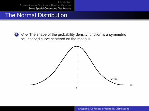
4 <1-> The shape of the probability density function is a symmetricbell-shaped curve centered on the mean µ


ieu.logo.png




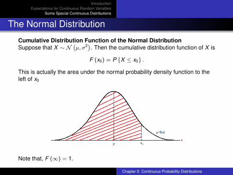
Cumulative Distribution Function of the Normal DistributionSuppose that X ∼ N

(µ, σ2). Then the cumulative distribution function of X is

F (x0) = P {X ≤ x0} .

This is actually the area under the normal probability density function to theleft of x0

Note that, F (∞) = 1.


ieu.logo.png




Let X be a normal random variable with cumulative distribution function F (x)and let a and b be two possible values of the random variable X with a < b.Then

P {a ≤ X ≤ b} = F (b)− F (a) .


ieu.logo.png



The Standard Normal Distribution

Definition:

Let Z be a normal random variable with mean 0 and variance 1, that is,Z ∼ N (0, 1). We say that Z follows a standard normal distribution. If thecumulative distribution function of Z is F (z) and a and b are two possiblevalues of Z with a < b, then

P {a ≤ Z ≤ b} = F (b)− F (a) .


ieu.logo.png



The Standard Normal DistributionWe can obtain probabilities for any normally distributed random variable by

first converting the random variable to the standard normally distributedrandom variable Z using the transformation

Z =X − µσ

,

where X ∼ N(µ, σ2),

then using the standard normal distribution table:


ieu.logo.png



The Standard Normal DistributionThe standard normal distribution table gives the values of F (z) = P {Z ≤ z}for nonnegative values of z. For example, F (1.25) = P {Z ≤ 1.25} = 0.8944


ieu.logo.png




and it is actually the area of the shaded region


ieu.logo.png




To find the cumulative probability for a negative z we use the complement ofthe probability of the positive value of this negative z. From symmetry, wehave

F (−z) = P {Z ≤ −z} = P {Z > z} = 1− P {Z ≤ z} = 1− F (z) .

For example, F (−1) = 1− F (1) = 1− 0.8413 = 0.1587 gives the area of


ieu.logo.png




Example. Find the area under the standard normal curve that lies

a) to the left of z = 2.5,

b) to the left of z = −1.55,

c) between z = −0.78 and z = 0,

d) between z = 0.33 and z = 0.66.


ieu.logo.png




Example. A random variable has a normal distribution with µ = 69 andσ = 5.1. What are the probabilities that the random variable will take a value

a) less than 74.1?

b) greater than 63.9?

c) between 69 and 72.3?

d) between 66.2 and 71.8?


ieu.logo.png




Example. A very large group of students obtains test scores that arenormally distributed with mean 60 and standard deviation 15. Find the cutoffpoint for the top 10% of all students for the test scores.


ieu.logo.png




Example. A random variable has a normal distribution with variance 100.Find its mean if the probability that it will take on a value less than 77.5 is0.8264.


ieu.logo.png



Normal Distribution Approximation for BinomialDistribution

Normal distribution can be used to approximate the discrete binomialdistribution. This approximation allows to compute probabilities for largersample sizes when tables are not available.

Consider a problem with n independent trials each with the probability ofsuccess p. The binomial random variable X can be written as the sum of nindependent Bernoulli random variables

X = X1 + X2 + · · ·+ Xn,

where Xi takes the value 1 if the outcome of the i th trial is “success ”and 0otherwise, with respective probabilities p and 1− p. Thus, X has binomialdistribution with mean and variance

E (X ) = µ = np and Var (X ) = σ2 = np(1− p).


ieu.logo.png




If the number of trials (n) is large so that np (1− p) > 5, then the distributionof the random variable

Z =X − µσ

=X − np√np(1− p)

is approximately a standard normal distribution.


ieu.logo.png




Example. An election forecaster has obtained a random sample of 900voters in which 500 indicate that they will vote for Susan Chung. Assumingthat there are only two candidates, should Susan Chung anticipate winningthe election?


ieu.logo.png



Proportion Random Variable

Definition:

A proportion random variable, P, can be computed by dividing the number ofsuccesses (X ) by the sample size (n):

P =Xn

Then, the mean and variance of P are

E (P) = µ = p and Var (P) = σ2 =p(1− p)

n.


ieu.logo.png



Proportion Random Variable

Example. An election forecaster has obtained a random sample of 900voters in which 500 indicate that they will vote for Susan Chung. Assumingthat there are only two candidates, should Susan Chung anticipate winningthe election? Solve using proportion random variable.


ieu.logo.png



The Exponential Distribution

The exponential distribution has been found particularly useful forwaiting-line, queueing, or lifetime problems.

Definition:

The exponential random variable T (T > 0) has a probability density function

f (t) = λe−λt for t > 0,

where lambda > 0 is the mean number of independent arrivals oroccurrences per time unit, t is the number of time units until the next arrival oroccurrence, and e = 2.71828 . . . .


ieu.logo.png




Let T be an exponential random variable. The cumulative distribution functionof T is

F (t0) = P {T ≤ t0} = 1− e−λt0 for t0 > 0.

The mean and variance of T are

E (T ) =1λ

and Var (T ) =1λ2 .


ieu.logo.png




Example. Service times for customers at a library information desk can bemodeled by an exponential distribution with a mean service time of 5minutes. What is the probability that a customer service time will take longerthan 10 minutes?


ieu.logo.png




Note: The Poisson distribution provides the probability of Xarrival/occurrences during a unit interval. In contrast, the exponentialdistribution provides the probability that an arrival/occurrence willoccur during an interval of time t .


ieu.logo.png




Example. An industrial plant in Britain with 2000 employees has a meannumber of lost-time accidents per week equal to λ = 0.4 and the number ofaccidents follows a Poisson distribution. What is the probability that the timebetween accidents is less than 2 weeks?


ieu.logo.png




Example. Times to gather preliminary information from arrivals at anoutpatient clinic follow an exponential distribution with mean 15 minutes. Findthe probability, for a chosen interval, that more than 18 minutes will berequired.


chapter 5: continuous probability distributions -...

Documents