chapter 4

Chapter 4: Non-Linear receivers

David Ramırez

Signal Processing GroupDepartment of Signal Theory and Communications

University Carlos III of Madrid

Signal Processing for CommunicationsWinter semester 2015/16

Motivation

MotivationConsider the estimation of x from the received signal

y = Hx+ n

I In digital communications, x is drawn from a constellation X .

I Linear receivers use only the mean and covariance matrix of x

I Non-linear receivers exploit information about the constellation to improvethe performance

Outline

1. Decision feedback (DF) estimation

2. Maximum likelihood (ML) estimation

3. Maximum a posteriori (MAP) estimation

DF Estimation

LMMSE DFE for ISI channels

A DFE scheme for single-antenna ISI channels: a feedforward filter (FFF) + afeedback filter (FBF) + a decision device

DFE for Multipath Channels

{yn}{wk}{bk}{xm}{dm}

Consider a sliding windowed DFE scheme for single-antenna multipathchannels, which include The DFE consists of the following three components: afeedforward filter (FFF), a feedback filter (FBF), and a decision device.

!

26 Channel equalization for dispersive channels

bl!m

dl

{fm}

{gm}FFF

devicedecision

FBF

yl !"

Figure 2.7. Structure of the DFE.

there are frequency nulls, as shown in Eq. (2.14), the corresponding frequency responses ofthe MMSE LE become zero to suppress the noise since there is no useful signal. Generally,if there are more frequency nulls, more corresponding frequency responses of the MMSELE become zero and this results in a worse performance of Channel A, as shown in Fig. 2.6.

2.3 Decision feedback equalizers

Depending on the channel spectrum, the performance of the LE varies. In particular, if thereare frequency nulls, the performance of the LE would not be satisfactory even though theSNR is high. To overcome this difficulty, the decision feedback equalizer (DFE) can be used.

The DFE consists of the following three components: a feedforward filter (FFF), afeedback filter (FBF), and a decision device. A block diagram for the DFE is depicted inFig. 2.7. In this section, we introduce a DFE with finite numbers of taps of FFF and FBF.The two criteria, ZF and MMSE, will be applied to derive the filter coefficients.

2.3.1 Zero-forcing DFE

Suppose that {gm} is the impulse response of the FFF and that the length of the impulseresponse is M . The convolution of the FFF’s impulse response {gm} and the channel impulseresponse {hp} becomes

cl =M!1!

m=0

gmhl!m . (2.15)

Using matrix notation, we can show that

c = [c0 c1 · · · cM+P!2]

= Hg

=

"

###$

h0 0 · · · 0h1 h0 · · · 0...

.... . .

...0 0 · · · h P!1

%

&&&'

( )* +(M+P!1)"M

g, (2.16)

Let n be the current time, D the decision delay, Kf and Kb be the lengths offeedforward and feedback filters, respectively. Let {wm} and {bm} be thefeedforward and feedback coefficients. The MSE is

MSE � E

��xn−D −

Kf−1�

k=0

w∗kyn−k −

Kb−1�

k=0

b∗kxn−D−k−1

��

2

Signal Processing for Wireless Communications Chapter 5: Nonlinear Receivers 4 / 14




!


bl!m

dl

{fm}

{gm}FFF

devicedecision

FBF

yl !"








cl =M!1!

m=0

gmhl!m . (2.15)


c = [c0 c1 · · · cM+P!2]

= Hg

=

"

###$

h0 0 · · · 0h1 h0 · · · 0...

.... . .

...0 0 · · · h P!1

%

&&&'

( )* +(M+P!1)"M

g, (2.16)


MSE � E

��xn−D −

Kf−1�

k=0

w∗kyn−k −

Kb−1�

k=0

b∗kxn−D−k−1

��

2





!


bl!m

dl

{fm}

{gm}FFF

devicedecision

FBF

yl !"








cl =M!1!

m=0

gmhl!m . (2.15)


c = [c0 c1 · · · cM+P!2]

= Hg

=

"

###$

h0 0 · · · 0h1 h0 · · · 0...

.... . .

...0 0 · · · h P!1

%

&&&'

( )* +(M+P!1)"M

g, (2.16)


MSE � E

��xn−D −

Kf−1�

k=0

w∗kyn−k −

Kb−1�

k=0

b∗kxn−D−k−1

��

2





!


bl!m

dl

{fm}

{gm}FFF

devicedecision

FBF

yl !"








cl =M!1!

m=0

gmhl!m . (2.15)


c = [c0 c1 · · · cM+P!2]

= Hg

=

"

###$

h0 0 · · · 0h1 h0 · · · 0...

.... . .

...0 0 · · · h P!1

%

&&&'

( )* +(M+P!1)"M

g, (2.16)


MSE � E

��xn−D −

Kf−1�

k=0

w∗kyn−k −

Kb−1�

k=0

b∗kxn−D−k−1

��

2





!


bl!m

dl

{fm}

{gm}FFF

devicedecision

FBF

yl !"








cl =M!1!

m=0

gmhl!m . (2.15)


c = [c0 c1 · · · cM+P!2]

= Hg

=

"

###$

h0 0 · · · 0h1 h0 · · · 0...

.... . .

...0 0 · · · h P!1

%

&&&'

( )* +(M+P!1)"M

g, (2.16)


MSE � E

��xn−D −

Kf−1�

k=0

w∗kyn−k −

Kb−1�

k=0

b∗kxn−D−k−1

��

2


+ -‐

Estimate of xm−D with DFE:

xm−D ,Kf−1∑

k=0

w∗kym−k −Kb−1∑

k=0

b∗kdm−D−k−1

Design {wk} and {bk} to minimize

MSE = E[|xm−D − xm−D|2

]

I D is the decision delay

I Kf and Kb are the lengths of FFF and FBF filters, respectively

I {wk} and {bk} are the FFF and FBF coefficients

LMMSE DFE for ISI channels (II)

Defining

w = [w0, w1, . . . , wKf−1]T

b = [b0, b1, . . . , bKb−1]T

ym = [ym, ym−1, . . . , ym−Kf+1]T

dm = [dm−D−1, dm−D−2, . . . , dm−D−Kb ]T

the MSE becomes

MSE = E

[∣∣∣xm−D −(wHym − bHdm

)∣∣∣2]= E

[∣∣∣∣∣xm−D −[w−b

]H [ymdm

]∣∣∣∣∣

2]

From the LMMSE principle, the optimal filters are

[w−b

]=

[E[ymyHm] E[ymdHm]E[dmyHm] E[dmdHm]

]−1 [E[ymx

∗m−D]

E[dmx∗m−D]

]

The difficulty lies in the complicated behavior of dm. We will assume error-freedecisions: dm = xm,∀m, to simplify problem

LMMSE DFE for ISI channels (III)

For DFE, the MSE is affected by decision errors

I With error-free decisions

MSE = E[|xm−D|2

]

−[E[ymx

∗m−D]

E[dmx∗m−D]

]H [E[ymyHm] E[ymdHm]E[dmyHm] E[dmdHm]

]−1 [E[ymx

∗m−D]

E[dmx∗m−D]

]

where dm = [xm−D−1, xm−D−2, · · · , xm−D−Kb ]T

I Propagation of the decisionerrors degrades the MSEperformance

0 5 10 15 20−22

−20

−18

−16

−14

−12

−10

−8

−6

−4

−2

SNR(dB)

MSE

(dB)

Error free bound for DFEDFE (simulation)LE (simulation)

LMMSE DFE for ISI channels (IV)

Example

Consider a real-valued system. The channel tap gains are h0 = 1 and h1 = 1/2.The noise is AWGN with variance σ2

n = 1/2. Let Kf = 2, Kb = 3 and{xm} ∈ {+1,−1} are i.i.d. with zero mean. Find the LMMSE DFE for D = 0.

Solution: The channel model is

ym = xm +1

2xm−1 + nm

Assuming error-free decisions

[E[ymyHm] E[ymdHm]E[dmyHm] E[dmdHm]

]=

74

12

12

0 012

74

1 12

012

1 1 0 00 1

20 1 0

0 0 0 0 1

[E[ymx

∗m]

E[dmx∗m]

]= [1, 0, 0, 0, 0]T

the optimal filters are w = [2/3, 0]T and b = [1/3, 0, 0]T , with MSE = 1/3

LMMSE DFE for MIMO systems

MIMO system model

y = Hx+ n,

where n and x are independent, have zero-mean and identity covariancematrices

Successive interference cancellation (SIC)

xM = wHMy

xM−1 = wHM−1(y − hMdM )

...

x1 = wH1 (y −

M∑

m=2

hmdm)

or in matrix form (assuming error-free decisions)

x = WHy −Bx = (WHH−B)x+WHn,

LMMSE DFE for MIMO systems (II)

+ _

+ _

+ _

+ _

This technique also suffers from error-propagation

LMMSE DFE for MIMO systems (III)Assuming detection in a decreasing order and error-free decisions, the estimateof the i symbol is

xi = wHi y −

M∑

j=i+1

bi,jxj , i =M,M − 1, . . . , 1

and the corresponding MSE becomes

MSEi = E[|xi−xi|2] = |wHi hi−1|2+

M∑

j=i+1

|wHi hj−bi,j |2+

i−1∑

j=1

|wHi hj |2+σ2

n||wi||2

Minimizing the MSE with respect to bi,j , we find that

bi,j = wHi hj , 1 ≤ i < j < M B = U(WHH)

where U(·) extracts the strictly upper triangular entries of a matrix, and theMSE becomes

MSEi = E[|xi − xi|2] = |wHi hi − 1|2 +

i−1∑

j=1

|wHi hj |2 + σ2

n||wi||2

Let Hi = [h1,h2, · · · ,hi], MSEi is minimized by

wi = (HiHHi + σ2

nI)−1hi, 1 ≤ i ≤M

LMMSE DFE for MIMO systems (IV)

Fast computations using QR factorization

Lemma: Let the economy-size QR factorization of the augmented matrix be

Hσ2n=

[Hσ2nI

]= QR =

[Q1

Q2

]R

where Q is unitary and R is upper triangular. The MMSE FFF and FBFmatrices are

W = Q1D−1R B = D−1

R R− I

where DR = diag(R). The resulting MSE matrix is diagonal

E = E[(x− x)(x− x)H ] = D−2R

SIC with optimal ordering

Instead of starting with the Mth symbol, we could start with the symbol withsmallest MSE to minimize the error-propagation effect.

LMMSE DFE for MIMO systems (V)

0 5 10 15 20−22

−20

−18

−16

−14

−12

−10

−8

−6

−4

SNR(dB)

MSE

(dB)

Error free bound for DFEDFE (simulation)LE (simulation)

A nT = 2, nR = 4 MIMO system over flat-fading channels with differentequalization schemes.

ML Estimation

Principles of ML estimation

Motivation

I LE or DFE separate the interference cancellation (estimation step) fromsymbol detection

I MLE detects symbol sequence directly

ML principle

System modely = Hx+ n

Given y the ML estimate maximizes the likelihood

x = arg maxx∈XM

p(y;x)

I We treat x as an unknown deterministic variable

I Since each entry of x belongs to a K-dimensional constellation, thecardinality of XM is |XM | = KM , and the complexity of ML detectionbecomes O(KM )

I Thus, one main problem is complexity reduction

ML estimation: An example

Consider a memoryless flat-fading channel with xm ∈ {+1,−1} and

ym = hxm + nm

where nm ∼ N (0, σ2n). Then, given xm, ym is a conditional Gaussian random

variable with

E[ym|xm] = hxm Var[ym|xm] = σ2n

Likelihood function

p(ym;xm) =1√2πσ2

n

exp

(− 1

2σ2n

(ym − hxm)2)

ML detector

xn =

{+1, if p(ym; +1) ≥ p(ym;−1)−1, if p(ym; +1) < p(ym;−1)

or, equivalently

xn =

{+1, if hym ≥ 0

−1, if hym < 0

The ML estimator exploits the finite constellation of xm

MLE in channels with ISI

A SISO channel with ISI

ym =

L−1∑

l=0

hlxm−l + nm, m = 0, 1, . . .

If the number of symbols is M , the aforementioned channel may bealternatively represented by y = Hx+ n, where x ∈ CM . The complexityO(|X |M ) can be prohibitively high

LikelihoodFor Gaussian noise, the likelihood becomes

p(y;x) ∝ exp

−

1

σ2n

M−1∑

m=0

∣∣∣∣∣ym −L−1∑

l=0

hlxm−l

∣∣∣∣∣

2

ML estimator

x = arg maxx∈XM

p(y;x) = arg min{xm},xm∈X

M−1∑

m=0

∣∣∣∣∣ym −L−1∑

l=0

hlxm−l

∣∣∣∣∣

2

︸︷︷︸V ({xm})

MLE in channels with ISI (II)

Example

L = 2, x0 = 0, and {y1, y2, y3, y4} = {2,−1, 4, 1},{h0, h1} = {1,−0.5}, xm ∈ {+1,−1}

Solution: By exhaustive search, the ML estimate is+1,−1,+1,+1

Symbol sequences Costs{+1,+1,+1,+1} 15.75{−1,+1,+1,+1} 27.75{+1,−1,+1,+1} 7.75{−1,−1,+1,+1} 15.75{+1,+1,−1,+1} 33.75{−1,+1,−1,+1} 45.75{+1,−1,−1,+1} 21.75{−1,−1,−1,+1} 29.75{+1,+1,+1,−1} 21.75{−1,+1,+1,−1} 33.75{+1,−1,+1,−1} 13.75{−1,−1,+1,−1} 21.75{+1,+1,−1,−1} 35.75{−1,+1,−1,−1} 47.75{+1,−1,−1,−1} 23.75{−1,−1,−1,−1} 31.75

MLE in channels with ISI (III)

Viterbi algorithm

I Efficient implementation of MLE

I Some definitions

ym = h0xm +

L−1∑

l=1

hlxm−l

I xm is the input and {Sm} = (xm−1, . . . , xm−L+1) is the channel state (ormemory)

I |X |L−1 possible states {Sk}I State transition occurs for each new input, forming a trellis diagram

I |X | branches leaving and entering each stateI Any data sequence is a path on the trellis diagram

Deteccion de secuencias ML usando la rejilla

Secuencia mas verosımil

A = arg mınai

N+L�1X

n=0

��

q[n] �NX

k=0

p[k]ai[n � k]

| {z }oi[n]

��

2

I Nuevas etiquetas en la rejilla - metrica de rama |q[n] � oi[n]|2I Verosimilitud para una secuencia: suma de las metricas de rama

de su camino a traves de la rejilla

u

u

u

u

u

u

u

u

u

u

u

u

-1

+1 . ..........................................................................................................................................................................................

........................

........................

........................

........................

........................

........................

........................

........................

........................

........................

........................

....... . .........................................................................................................................................................................................

.

................................................................................................................................................................................................................................................................................ .........................................................................................................................................................................................

.

........................

........................

........................

........................

........................

........................

........................

........................

........................

........................

........................

........ .........................................................................................................................................................................................

.

............................................................................................................................................................................................................................................................................... . .........................................................................................................................................................................................

.

........................

........................

........................

........................

........................

........................

........................

........................

........................

........................

........................

........ .........................................................................................................................................................................................

.

............................................................................................................................................................................................................................................................................... . .........................................................................................................................................................................................

.

........................

........................

........................

........................

........................

........................

........................

........................

........................

........................

........................

........ .........................................................................................................................................................................................

.

...............................................................................................................................................................................................................................................................................

q[0] = +0,5 q[1] = �0,4 q[2] = +0,1 q[3] = �1,7 q[4] = +0,3

1

1

3,61

0,01

0,81

1,21

1,96

0,36

0,16

2,56

10,24

1,44

4,84

0,04

1,44

0,04

c�Marcelino Lazaro, 2015 Comunicaciones Digitales Deteccion bajo ISI 36 / 141I VA finds the ML sequence on the trellis diagram

MLE in channels with ISI (IV)

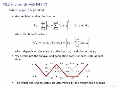
Viterbi algorithm (cont’d)

I Accumulated cost up to time m

Vn =

m∑

k=0

∣∣∣∣∣yk −L−1∑

l=0

hlxk−l

∣∣∣∣∣

2

= Vm−1 +Mm

where the branch metric is

Mm =M(xm, Sm; ym) =

∣∣∣∣∣ym −L−1∑

l=0

hlxn−l

∣∣∣∣∣

2

which depends on the state Sm, the input xm and the output ym

I VA determines the survival and competing paths for each state at eachtime

Deteccion de secuencias ML usando la rejilla

Secuencia mas verosımil

A = arg mınai

N+L�1X

n=0

��

q[n] �NX

k=0

p[k]ai[n � k]

| {z }oi[n]

��

2

I Nuevas etiquetas en la rejilla - metrica de rama |q[n] � oi[n]|2I Verosimilitud para una secuencia: suma de las metricas de rama

de su camino a traves de la rejilla

u

u

u

u

u

u

u

u

u

u

u

u

-1

+1 . ..........................................................................................................................................................................................

........................

........................

........................

........................

........................

........................

........................

........................

........................

........................

........................

....... . .........................................................................................................................................................................................

.

................................................................................................................................................................................................................................................................................ .........................................................................................................................................................................................

.

........................

........................

........................

........................

........................

........................

........................

........................

........................

........................

........................

........ .........................................................................................................................................................................................

.

............................................................................................................................................................................................................................................................................... . .........................................................................................................................................................................................

.

........................

........................

........................

........................

........................

........................

........................

........................

........................

........................

........................

........ .........................................................................................................................................................................................

.

............................................................................................................................................................................................................................................................................... . .........................................................................................................................................................................................

.

........................

........................

........................

........................

........................

........................

........................

........................

........................

........................

........................

........ .........................................................................................................................................................................................

.

...............................................................................................................................................................................................................................................................................

q[0] = +0,5 q[1] = �0,4 q[2] = +0,1 q[3] = �1,7 q[4] = +0,3

1

1

3,61

0,01

0,81

1,21

1,96

0,36

0,16

2,56

10,24

1,44

4,84

0,04

1,44

0,04

r

rrrrrrrrrrrrrrrrrrrrrrrrrrrrrrrrrrrrrrrrrrrrrrrrrrrrrr

rrrrrrrrrrrrrrrrrrrrrrrrrrrrrrrrrrrrrrrrrr


rrrrrrrrrrrrrrrrrrrrrrrrrrrrrrrrrrrrrrrrr

r

rrrrrrrrrrrrrrrrrrrrrrrrrrrrrrrrrrrrrrrrrrrrrrrrrrrrrrrrrrrrrrrrrrrrrrrrrrrrrrrrrrrrrrrrrrrrrrr

r


rrrrrrrrrrrrrrrrrrrrrrrrrrrrrrrrrrrrrrrrr

r rrrrrrrrrrrrrrrrrrrrrrrrrrrrrrrrrrrrrrrrrrrrrrrrrrrrrrrrrrrrrrrrr r

rrrrrrrrrrrrrrrrrrrrrrrrrrrrrrrrrrrrrrrrrrrrrrrrrrrrrrrrrrrrrrrrrrrrrrrrrrrrrrrrrrrrrrrrrrrrrrr2,25

c�Marcelino Lazaro, 2015 Comunicaciones Digitales Deteccion bajo ISI 37 / 141I The initial and ending states are determined by the transmission scheme

MAP Estimation

Principles of MAP estimation

Motivation

I LMMSE-LE and LMMSE-DFE utilize only second-order statistics and theconstellation

I ML estimation utilizes only likelihood function

I MAP estimation uses a priori information to further improve performance,and hence minimizes symbol error rate

MAP principle

System modely = Hx+ n

MAP estimator maximizes the a posteriori probability (APP)

xMAPm = argmax

xmPr(xm|y), m = 0, 1, . . . ,M − 1

or, equivalently, (via Bayes’ rule)

xMAPm = argmax

xmp(y|xm)p(xm)

MAP in channels with ISI

Considering a BPSK transmission and a frequency selective SISO channel

ym =

L−1∑

l=0

hlxm−l + nm

the MAP estimate for xm is

xm = arg maxxm∈{+1,−1}

Pr(xm|y) ={+1, if Pr(xm = +1|y) ≥ Pr(xm = −1|y)−1, if Pr(xm = +1|y) < Pr(xm = −1|y)

The estimate is alternatively determined by the sign of the log-ratio of APP

xm = sign

(log

Pr(xm = +1|y)Pr(xm = −1|y)

)

Implementation based on exhaustive search has exponential complexity since

Pr(xm = +1|y) = C∑

{x:xm=+1}p(y|x) Pr(x)

requires the computation of 2M−1 terms. BCJR algorithm (due to Bahl,Cocke, Jelinek and Raviv) is a computationally efficient MAP algorithm formodels with trellis structure

chapter 4

Documents

afeedforward filter

filter coefficients

sliding windowed dfe

isi channelsa dfe scheme

decision devicedfe

decision delay

feedback coecients

feedback filters