chapter 25 geomorphometry and spatial hydrologic … · · 2013-08-15462 geomorphometry and...

Chapter 25

Geomorphometry and spatial hydrologic

modelling

Peckham, S.D.1

how can DEMs be used for spatial2

hydrologic modelling? • what methods3

are commonly used to model hydrologic4

processes in a watershed? • what kinds5

of preprocessing tools are typically6

required? • what are some of the key7

issues in spatial hydrologic modelling?8

25.1 Introduction9

Spatial hydrologic modelling is one of the10

most important applications of the geomorpho-11

metric concepts discussed in this book. The sim-12

ple fact that flow paths follow the topographic13

gradient results in an intimate connection be-14

tween geomorphometry and hydrology, and this15

connection has driven much of the progress in16

the field of geomorphometry. It also continues17

to help drive the development of new technolo-18

gies for creating high-quality and high-resolution19

DEMs, such as LiDAR. Like most other types of20

physically-based models, hydrologic models are21

built upon the fundamental principle that the22

mass and momentum of water must be conserved23

as it moves from place to place, whether it is on24

the land surface, below the surface or evaporat-25

ing into the atmosphere. While this sounds like26

a simple enough idea, it provides a powerful con-27

straint that makes predictive modelling possible.28

When mass and momentum conservation is sim-29

ilarly applied to sediment, it is possible to create30

landscape evolution models that predict the31

spatial erosion and deposition of sediment and 32

contaminants. 33

While hydrologic models have been around 34

for several decades, it is only in the last fifteen 35

years or so that computers have become powerful 36

enough for fully spatial hydrologic models to be 37

of practical use. Spatially-distributed hydro- 38

logic models treat every grid cell in a DEM as a 39

control volume which must conserve both mass 40

and momentum as water is transported to, from, 41

over and below the land surface. The control vol- 42

ume concept itself is quite simple: what flows in 43

must either flow out through another face or ac- 44

cumulate or be consumed in the interior. Con- 45

versely, the amount that flows out during any 46

given time step cannot exceed the amount that 47

flows in during that time step plus the amount al- 48

ready stored inside. However, the number of grid 49

cells required to adequately resolve the transport 50

within a river basin, in addition to the small size 51

of the timesteps required for a spatial model to 52

be numerically stable, results in a computational 53

cost that until recently was prohibitive. 54

Remark 118: Since flow paths follow the

topographic gradient, there is an intimate

connection between geomorphometry and

hydrology. Spatial hydrologic models make

use of several DEM-derived grids especially

grids of slope, aspect (flow direction) and

contributing area.

55

56

For a variety of reasons, including the com- 57

putational cost of fully spatial models and the 58

461

462 Geomorphometry and spatial hydrologic modelling

fact that data required for more advanced mod-1

els is often unavailable, researchers have invested2

a great deal of effort into finding ways to sim-3

plify the problem. This has resulted in many4

different types of hydrologic models. For ex-5

ample, lumped models employ a small num-6

ber of “representative units” (very large, but7

carefully-chosen control volumes), with simple8

methods to route flow between the units. An-9

other strategy for reducing the complexity of hy-10

drologic models is to use concepts such as hy-11

drologic similarity to essentially collapse the12

2D (or 3D) problem to a 1D problem. For ex-13

ample, TOPMODEL (Beven and Kirkby, 1979)14

defines a topographic index or wetness in-15

dex and then lumps all grid cells with the same16

value of this index together under the assump-17

tion that they will have the same hydrologic re-18

sponse. Similarly, many models lump together19

all grid cells with the same elevation (via the20

hypsometric curve or area-altitude func-21

tion) to simplify the problem of computing cer-22

tain quantities such as snowmelt. All grid cells23

with a given flow distance to a basin outlet can24

also be lumped together (via the width func-25

tion or area-distance function) and this is the26

main idea behind the concept of the instanta-27

neous unit hydrograph. While models such28

as these can be quite useful and require less in-29

put data, they all employ simplifying assump-30

tions that prevent them from addressing general31

problems of interest. In addition, these assump-32

tions are often difficult to check and are therefore33

a source of uncertainty. In essence, these types34

of models gain their speed by mapping many dif-35

ferent (albeit similar) 3D flow problems to the36

same 1D problem in the hope that the lost differ-37

ences don’t matter much. While geomorphome-38

tric grids are used to prepare input data for vir-39

tually all hydrologic models, fully spatial models40

make direct use of these grids. For this reason,41

and in order to limit the scope of the discussion,42

this chapter will focus on fully-spatial models.43

There are now many different spatial hydro-44

logic models available, and their popularity, so-45

phistication and ease-of-use continues to grow46

with every passing year. A few representa-47

tive examples of some highly-developed spa- 48

tial models are: Mike SHE (a product of 49

Danish Hydraulics Institute, Denmark), Grid- 50

ded Surface Subsurface Hydrologic Analysis 51

(GSSHA), CASC2D (Julien et al., 1995; Og- 52

den and Julien, 2002), PRMS (Leavesley et al., 53

1991), DHVSM (Wigmosta et al., 1994) and 54

TopoFlow. Rather than attempt to review or 55

compare various models, the main goal of this 56

chapter is to discuss basic concepts that are com- 57

mon to virtually all spatial hydrologic models. 58

Remark 119: Hydrologic processes in a

watershed (e.g. snowmelt) may be modelled

with either simple methods (e.g. degree-

day) or very sophisticated methods (e.g.

energy-balance), based partly on the input

data that is available.

59

60

It will be seen throughout this chapter that 61

grids of elevation, slope, aspect and contribut- 62

ing area all play fundamental roles in spatial hy- 63

drologic modelling. Some of these actually play 64

multiple roles. For example, slope and aspect are 65

needed to determine the velocity of surface (and 66

subsurface) flow, but also determine the amount 67

of solar radiation that is available for evapotran- 68

spiration and melting snow. The DEM grid spac- 69

ing that is required depends on the application, 70

but as a general rule should be sufficient to ad- 71

equately resolve the local hillslope scale. This 72

scale marks the transition in process dominance 73

from hillslope processes to channel processes. It 74

is typically between 10 and 100 m, but may be 75

larger for arid regions. As a result of the Shut- 76

tle Radar Topography Mission (SRTM), DEMs 77

with a grid spacing less than 100 m are now avail- 78

able for much of the Earth. In addition, LiDAR 79

DEMs with a grid spacing less than 10 m can 80

now be purchased from private firms for specific 81

areas. Many of the DEMs produced by govern- 82

ment agencies (e.g. the U.S. Geological Survey 83

and Geoscience Australia) now use an algorithm 84

such as ANUDEM (Hutchinson, 1989) to produce 85

“hydrologically sound” DEMs which makes them 86

25.2 Spatial hydrologic modelling: processes and methods 463

better suited to hydrologic applications (see also1

§2.3.2).2

This chapter has been organised as follows.3

§25.2 discusses several key hydrologic processes4

and how they are typically incorporated into spa-5

tial models. Note that spatial hydrologic models6

integrate many branches of hydrology and there7

are many different approaches for modelling any8

given process, from simple to very complex. It9

is therefore impossible to give a complete treat-10

ment of this subject in this chapter. For a greater11

level of detail the reader is referred to textbooks12

and monographs such as (Henderson, 1966; Ea-13

gleson, 1970; Freeze and Cherry, 1979; Welty14

et al., 1984; Beven, 2000; Dingman, 2002; Smith,15

2002). The goal here is to highlight the most16

fundamental concepts that are common between17

spatial models and to show how they incorporate18

geomorphometric grids. §25.3 discusses scale is-19

sues in spatial hydrologic modelling. §25.4 pro-20

vides a brief discussion of preprocessing tools21

that are typically needed in order to prepare re-22

quired input data. §25.5 is a simple case study in23

which a model called TopoFlow is used to simu-24

late the hydrologic response of a small ungauged25

watershed in the Baranja Hill case study.26

25.2 Spatial hydrologic modelling:27

processes and methods28

25.2.1 The control volume concept29

Spatially-distributed hydrologic models are30

based on applying the control volume concept31

to every grid cell in a digital elevation model32

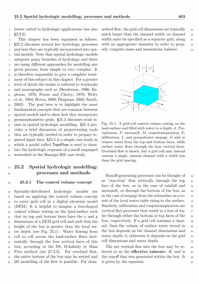
(DEM). It is helpful to imagine a box-shaped33

control volume resting on the land-surface such34

that its top and bottom faces have the x and y35

dimensions of a DEM grid cell and such that the36

height of the box is greater than the local wa-37

ter depth (see Fig. 25.1). Water flowing from38

cell to cell across the land-surface flows hori-39

zontally through the four vertical faces of this40

box, according to the D8, D-Infinity or Mass41

Flux method (see §7.3.2). For overland flow,42

the entire bottom of the box may be wetted and43

2D modelling of the flow is possible. For chan-44

nelised flow, the grid cell dimensions are typically 45

much larger than the channel width, so channel 46

width must be specified as a separate grid, along 47

with an appropriate sinuosity in order to prop- 48

erly compute mass and momentum balance. 49

Fig. 25.1: A grid-cell control volume resting on the

land-surface and filled with water to a depth, d. Pre-

cipitation, P , snowmelt, M , evapotranspiration, E,

infiltration, I, and groundwater seepage, G add or

remove water from the top and bottom faces, while

surface water flows through the four vertical faces.

Overland flow is shown, but a grid cell may instead

contain a single, sinuous channel with a width less

than the grid spacing.

Runoff-generating processes can be thought of 50

as “injecting” flow vertically through the top 51

face of the box, as in the case of rainfall and 52

snowmelt, or through the bottom of the box, as 53

in the case of seepage from the subsurface as a re- 54

sult of the local water table rising to the surface. 55

Similarly, infiltration and evapotranspiration are 56

vertical flux processes that result in a loss of wa- 57

ter through either the bottom or top faces of the 58

box, respectively. If a grid cell contains a chan- 59

nel, then the volume of surface water stored in 60

the box depends on the channel dimensions and 61

water depth, d, otherwise it depends on the grid 62

cell dimensions and water depth. 63

The net vertical flux into the box may be re- 64

ferred to as the effective rainrate, R, and is 65

the runoff that was generated within the box. It 66

is given by the equation: 67


R = (P +M +G)− (E + I) (25.2.1)

where P is the precipitation rate, M is snowmelt1

rate, G is the rate of subsurface seepage, E is the2

evapotranspiration rate and I is the infiltration3

rate.4

Each of these six quantities varies both spa-5

tially and in time and is therefore stored as a grid6

of values that change over time. Each also has7

units of [mm/hr]. Methods for computing these8

quantities are outlined in the next few subsec-9

tions of this chapter. Note that the total runoff10

from the box is not equivalent to the effective11

rainrate because it consists of the effective rain-12

rate plus any amount that flowed horizontally13

into the box and was not consumed by infiltra-14

tion or evapotranspiration. Note also that in or-15

der to model the details of subsurface flow, it is16

necessary to work with an additional “stack” of17

boxes that extend down into the subsurface; e.g.18

there may be one such box for each of several soil19

layers.20

In many models of fluid flow, fluxes through21

control volume boundaries (e.g. the vertical faces22

of the box) are not computed directly. Instead,23

the boundary integrals are converted to integrals24

over the interior of the box using the well-known25

divergence theorem (Welty et al., 1984). This26

results in differential vs. integral equations and27

requires computing first and second-order spa-28

tial derivatives between neighboring cells, typi-29

cally via finite-difference methods. However, if30

we assume that flow directions are determined31

by topography, which is a relatively static quan-32

tity, then flow directions between grid cells are33

fixed and known at the start of a model run.34

Under these circumstances it is straight-forward35

and efficient to compute boundary integrals.36

25.2.2 The precipitation process37

The precipitation process differs from most of38

the other hydrologic processes at work in a basin39

in that the precipitation rate must be speci-40

fied either from measurements (e.g. radar or rain41

gauges) or as the result of numerical simulation.42

All of the other processes are concerned with 43

methods for tracking water that is already in 44

the system as it moves from place to place (e.g. 45

cell to cell or between surface and subsurface). 46

For a small catchment, it may be appropriate to 47

use measured rainrates from a single gauge for 48

all grid cells. For larger catchments and greater 49

realism, however, it is better to use space-time 50

rainfall, which is stored as a grid stack, indexed 51

by time. This grid stack may be created by spa- 52

tially interpolating data from many different rain 53

gauges. Input data for air temperature (T ) is 54

used to determine whether precipitation falls as 55

rain or as snow. 56

In order to model how temperature decreases 57

with increasing elevation, a grid of elevations can 58

be used together with a lapse rate. If precipi- 59

tation falls as snow (T <0 °C), then it can be 60

stored as a grid of snow depths that can change 61

in time. If the snowmelt process is modelled, 62

then snowmelt can contribute runoff to any grid 63

cell that has a nonzero snow depth and an air 64

temperature greater than 0 °C. 65

25.2.3 The snowmelt process 66

In general, the conversion of snow to liquid wa- 67

ter is a complex process that involves a detailed 68

exchange of energy in its various forms between 69

the atmosphere and the snowpack. While air 70

temperature is obviously of key importance, nu- 71

merous other variables affect the meltrate, in- 72

cluding the slope and aspect of the topography, 73

wind speed and direction, the heights of rough- 74

ness elements (e.g. vegetation) and the snow den- 75

sity to name a few. The Energy Balance 76

Method (Marks and Dozier, 1992; Liston, 1995; 77

Zhang et al., 2000) in its various implementa- 78

tions is therefore the most sophisticated method 79

for melting snow, but it is very data intensive. 80

This method consists of numerous equations (see 81

references) and generally makes use of a clear- 82

sky radiation model (see §8.3.1; Dozier (1980) 83

or Dingman (2002, Appendix E)), for modelling 84

the shortwave solar radiation and the Stephan- 85

Boltzmann law for modelling the longwave ra- 86

diation. Most clear-sky radiation models incor- 87


porate topographic effects via slope and aspect1

grids extracted from DEMs.2

width

roughness: n or z0theta

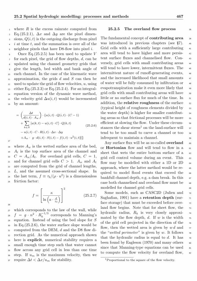
Fig. 25.2: A channel with a trapezoidal cross-section

and roughness elements that would connect the cen-

ters of two DEM grid cells. The cross-section be-

comes triangular when the bed width is zero and

rectangular when the bank angle is zero.

Since the input data required for energy3

balance calculations is only available in well-4

instrumented watersheds, much simpler meth-5

ods for estimating the rate of snowmelt have6

been developed such as various forms of the well-7

known Degree-Day Method (Beven, 2000,8

p.80). The basic method predicts the meltrate9

using the simple formula:10

M = c0 ·∆T (25.2.2)

where ∆T is the temperature difference between11

the air and the snow and c0 is an empirical co-12

efficient with units of [mm/hr/°C]. In both the13

Degree-Day and Energy-Balance methods it is14

possible for any input variable to vary spatially15

and in time, and many authors suggest that c016

should vary throughout the melt season. An17

example comparison of these two methods is18

given by Bathurst and Cooley (1996). What-19

ever method is used, the end result is a grid se-20

quence of snowmelt rates, M , that is then used21

in Eq.(25.2.1).22

25.2.4 The channel flow process23

Spatial hydrologic models are based on conserva-24

tion of mass and momentum, and many of them25

make direct use of D8 flow direction grids and26

slope grids to compute the amount of mass and 27

momentum that flows into and out of each grid 28

cell. The grid cell size is generally chosen to be 29

smaller than the hillslope scale and larger than 30

the width of the largest channel (see §25.3). Ev- 31

ery grid cell then has one channel associated with 32

it that extends from the centre of the grid cell to 33

the centre of the grid cell that it flows to accord- 34

ing to the D8 method. Channelised flow is then 35

modelled as an essentially 1D process (in a tree- 36

like network of channels), while recognising that 37

it will be necessary to store additional channel 38

properties for every grid cell such as: 39

sinuosity or channel length; 40

channel bed width; 41

bank angle (if trapezoidal cross sections are 42

used) and; 43

a channel roughness parameter. 44

One method for creating these channel property 45

grids is discussed in §25.4. 46

The kinematic wave method is the simplest 47

method for modelling flow in open channels and 48

is available as an option in virtually all spatial 49

hydrologic models. This method combines mass 50

conservation with the simplest possible treat- 51

ment of momentum conservation, namely that 52

all terms in the general momentum equation 53

(pressure gradient, local acceleration and convec- 54

tive acceleration) are neglible except the friction 55

and gravity terms. In this case the water surface 56

slope, energy slope and bed slope are all equal. 57

In addition, the balance of gravity against fric- 58

tion (as a shear stress near the bed) results in an 59

equation for depth-averaged flow velocity, u, in 60

terms of the flow depth, d, bed slope (rise over 61

run), S, and a roughness parameter. If the shear 62

stress near the bed is computed using our best 63

theoretical understanding of turbulent boundary 64

layers (Schlicting, 1960), then this balance re- 65

sults in the law of the wall: 66

u = (g ·Rh · S)1/2 · ln(a · d

z0

)· κ−1 (25.2.3)


Here, g is the gravitational constant, Rh is1

the hydraulic radius, given as the ratio of the2

wetted cross-sectional area and wetted perime-3

ter (units of length), a is an integration constant4

(given by 0.368 or 0.476, depending on the for-5

mulation), z0 is the roughness height (units6

of length), and κ ≈ 0.408 is von Karman’s con-7

stant.8

Note that the law of the wall is general and is9

also used by the snowmelt energy-balance mod-10

els for modelling air flow in the atmospheric11

boundary layer. However, in the setting of open-12

channel flow, an alternative known as Man-13

ning’s formula is more often used. Man-14

ning’s formula, which was determined by fitting15

a power-law to data gives the depth-averaged ve-16

locity as:17

u =R

2/3h · S1/2

n(25.2.4)

where n is an empirical roughness parameter18

with the units of [s/m1/3] required to make the19

equation dimensionally consistent. Manning’s20

formula agrees very well with the law of the wall21

as long as the relative roughness, z0/d is between22

about 10−2 and 10−4. This is the range that23

is encountered in most open-channel flow prob-24

lems. Smaller relative roughnesses are typically25

encountered in the case where wind blows over26

terrain and vegetation. ASCE Task Force on27

Friction Factors (1963) provides a good review28

of the long and interesting history that led to29

equations Eq.(25.2.3) and Eq.(25.2.4).30

While the kinematic wave method is an ap-31

proximation, it often yields good results, espe-32

cially when slopes are steep. The diffusive33

wave method provides a somewhat better ap-34

proximation by retaining one additional term in35

the momentum equation, namely the pressure-36

gradient (water depth derivative) term. In this37

method, the slope of the free water surface is38

used instead of the bed slope, and pressure-39

related (e.g. backwater) effects can be modelled.40

Note that a general treatment of momentum con-41

servation uses the full St. Venant equation,42

which includes the effects of gravity, friction and43

pressure-gradients as well as terms for local and44

convective acceleration. The convective acceler- 45

ation term corresponds to the net flux of momen- 46

tum into a given control volume. The most ac- 47

curate but most computationally demanding ap- 48

proach retains all of the terms in the St. Venant 49

equation and is known as the dynamic wave 50

method. Interestingly, the latter two methods 51

create a water-depth gradient and can thereby 52

move water across flat areas (e.g. lakes) in a 53

DEM. These areas have a bed slope of zero and 54

therefore receive a velocity of zero in the kine- 55

matic wave method unless they are handled sep- 56

arately in some manner. Whether the kinematic, 57

diffusive or dynamic wave method is used, it is 58

necessary to compute a grid of bed slopes. Given 59

a DEM with sufficient vertical resolution, the 60

bed slope can be computed between each grid 61

cell and its downstream neighbour, as indicated 62

by a D8 flow grid (see §7). 63

The D8 flow direction grid indicates the 64

(static) connectivity of the grid cells in a DEM 65

and can therefore be used directly to simplify 66

mass and momentum balance calculations. A 67

D8 flow grid allows fluxes across grid cell bound- 68

aries to be computed, which makes it possible 69

to use integral equations instead of differential 70

equations (Welty et al., 1984). In particular, the 71

use of integral equations is simpler because con- 72

vective acceleration (momentum flux) between 73

cells can be modelled without computing spatial 74

derivatives. Grids for the initial flow depth, d, 75

and velocity, u, are specified, either as all zeros 76

or computed from channel properties and a base- 77

level recharge rate. Given the cross-sectional 78

shape (e.g. trapezoidal) and length, L, of each 79

channel, the volume of water in the channel 80

can be computed as V = Ac · L, where Ac is 81

the cross-sectional area. An outgoing discharge, 82

Q = u · Ac, can also be computed for every grid 83

cell. For each time step, the change in volume 84

∆V (i, t) for pixel i can then be computed as: 85

= ∆t ·

24R(i, t) ·∆x ·∆y −Q(i, t) +

Xk∈N

Q(k, t)

35

(25.2.5)

86


where R is the excess rainrate computed from1

Eq.(25.2.1), ∆x and ∆y are the pixel dimen-2

sions, Q(i, t) is the outgoing discharge from pixel3

i at time t, and the summation is over all of the4

neighbor pixels that have D8-flow into pixel i.5

Once Eq.(25.2.5) has been used to update V6

for each pixel, the grid of flow depths, d, can be7

updated using the channel geometry grids that8

give the length, bed width and bank angle of9

each channel. In the case of the kinematic wave10

approximation, the grids d and S can then be11

used to update the grid of flow velocities, u, using12

either Eq.(25.2.3) or Eq.(25.2.4). For an integral-13

equation version of the dynamic wave method,14

the velocity grid ∆u(i, t) would be incremented15

by an amount:16

=

�∆t

d(i, t) ·Aw

�· {u(i, t) ·Q(i, t) · (C − 1)

+Xk∈N

[u(k, t)− u(i, t) · C] ·Q(k, t)

− u(i, t) · C ·R(i, t) ·∆x ·∆y

+Aw ·�g · d(i, t) · S(i, t)− f(i, t) · u2(i, t)

�(25.2.6)

17

where Aw is the wetted surface area of the bed,18

At is the top surface area of the channel and19

C = Aw/At. For overland grid cells, C = 1,20

and for channel grid cells C > 1. Aw and At21

are computed from the grid of channel lengths,22

L, and the assumed cross-sectional shape. In23

the last term, f ≡ τb/(ρ · u2) is a dimensionless24

friction factor:25

f =

κ

ln(a · d

z0

)2

(25.2.7)

26

which corresponds to the law of the wall, while27

f = g · n2 · R−1/3h corresponds to Manning’s28

equation. Instead of using the bed slope for S29

in Eq.(25.2.6), the water surface slope would be30

computed from the DEM, d and the D8 flow di-31

rection grid. As the numerical approach shown32

here is explicit, numerical stability requires a33

small enough time step such that water cannot34

flow across any grid cell in less than one time35

step. If um is the maximum velocity, then we36

require ∆t < ∆x/um for stability.37

25.2.5 The overland flow process 38

The fundamental concept of contributing area 39

was introduced in previous chapters (see §7). 40

Grid cells with a sufficiently large contributing 41

area will tend to have higher and more persis- 42

tent surface fluxes and channelised flow. Con- 43

versely, grid cells with small contributing areas 44

will tend to have lower, intermittent fluxes. The 45

intermittent nature of runoff-generating events, 46

and the increased likelihood that small amounts 47

of water will be fully consumed by infiltration or 48

evapotranspiration make it even more likely that 49

grid cells with small contributing areas will have 50

little or no surface flux for much of the time. In 51

addition, the relative roughness of the surface 52

(typical height of roughness elements divided by 53

the water depth) is higher for smaller contribut- 54

ing areas so that frictional processes will be more 55

efficient at slowing the flow. Under these circum- 56

stances the shear stress1 on the land-surface will 57

tend to be too small to carve a channel or too 58

infrequent to maintain a channel. 59

Any surface flux will be as so-called overland 60

or Hortonian flow and will tend to flow in a 61

sheet that wets the entire bottom surface of a 62

grid cell control volume during an event. This 63

flow may be modelled with either a 1D or 2D 64

approach, where the latter method would be re- 65

quired to model flood events that exceed the 66

bankfull channel depth, e.g. a dam break. In this 67

case both channelised and overland flow must be 68

modelled for channel grid cells. 69

Some models, such as CASC2D (Julien and 70

Saghafian, 1991) have a retention depth (sur- 71

face storage) that must be exceeded before over- 72

land flow begins. Note that for sheet flow, the 73

hydraulic radius, Rh is very closely approxi- 74

mated by the flow depth, d. If w is the width 75

of the grid cell projected in the direction of the 76

flow, then the wetted area is given by w d and 77

the “wetted perimeter” is given by w. It follows 78

that the hydraulic radius is equal to d. It has 79

been found by Eagleson (1970) and many others 80

since that Manning-type equations can be used 81

to compute the flow velocity for overland flow, 82

1Proportional to the square of the flow velocity.


but that a very large “Manning’s n” value of1

around 0.3 or higher is required, versus a typical2

value of 0.03 for natural channels.3

25.2.6 The evaporation process4

Evaporation is a complex, essentially vertical5

process that moves water from the Earth’s sur-6

face and subsurface to the atmosphere. As with7

the snowmelt process, the most sophisticated ap-8

proach is based on a full surface energy balance9

in which topographic effects can be incorporated10

by including grids of slope and aspect in the solar11

radiation model. However, since much of the re-12

quired input data is typically unavailable, a num-13

ber of simpler models have been proposed. The14

Priestley-Taylor (Priestley and Taylor, 1972;15

Rouse and Stewart, 1972; Rouse et al., 1977;16

Zhang et al., 2000) and Penman-Monteith17

models (Beven, 2000; Dingman, 2002) and their18

variants are two simplified approaches that are19

used widely. Sumner and Jacobs (2005) provide20

a comparison of these and other methods.21

Whatever method is used, the end result is22

a grid sequence of evapotranspiration rates, E,23

that is then used in Eq.(25.2.1). Some dis-24

tributed hydrologic models have additional rou-25

tines for modelling the amount of water that is26

moved from the root zone of the subsurface to27

the atmosphere by the transpiration of plants.28

A separate submodel is sometimes used to model29

the variation of soil temperature with depth, es-30

pecially for high-latitude applications.31

25.2.7 The infiltration process32

The process of infiltration is also primarily verti-33

cal, but is arguably the most complex hydrologic34

process at work in a basin. It has a first-order35

effect on the hydrologic response of watersheds,36

and is central to problems involving surface soil37

moisture. It operates in the unsaturated zone38

between the surface and the water table and rep-39

resents an interplay between absorption due to40

capillary action and the force of gravity. A vari-41

ety of factors make realistic modelling of infiltra-42

tion difficult, including the nature of boundary43

conditions at the surface, between soil layers and 44

at the water table (a moving boundary). Vari- 45

ables such as hydraulic conductivity can vary 46

over orders of magnitude in both space and time 47

and the equations are strongly nonlinear. 48

As pointed out by many authors, including 49

Smith (2002), it is generally not sufficient to sim- 50

ply use spatial averages for input parameters, 51

and best methods for parameter estimation are 52

an active area of research. So-called macropores 53

may be present and must then be modelled sepa- 54

rately since they do not conform to the standard 55

notion of a porous medium. Discontinuous per- 56

mafrost may also be present in high-latitude wa- 57

tersheds. Smith (2002) provides an excellent ref- 58

erence for infiltration theory, ranging from very 59

simple to advanced approaches. 60

Most spatial hydrologic models use a variant of 61

the Green-Ampt or Smith-Parlange method 62

for modelling infiltration (Smith, 2002). How- 63

ever, these are simplified approaches that are in- 64

tended for the relatively simple case where there 65

is: 66

a single storm event, 67

a single soil layer and 68

no water table 69

While they can be useful for predicting flood 70

runoff, they are not able to address many other 71

problems of contemporary interest, such as: 72

1. redistribution of the soil moisture profile be- 73

tween runoff-producing events, 74

2. drying of surface layers due to evaporation 75

at the surface, 76

3. rainfall rates less than Ks (saturated hy- 77

draulic conductivity), 78

4. multiple soil layers with different properties, 79

and 80

5. the presence of a dynamic water table. 81

In order to address these issues and to model sur- 82

face soil moisture a more sophisticated approach 83

is required. 84


Infiltration in a porous medium is modelled1

with four basic quantities which vary spatially2

throughout the subsurface and with time. The3

water content (θ) is the fraction of a given vol-4

ume of the porous medium that is occupied by5

water, and must therefore always be less than6

the porosity, φ. In the case of soils, θ repre-7

sents the soil moisture. The pressure head8

(or capillary potential), ψ, is negative in the un-9

saturated zone and measures the strength of the10

capillary action. It is zero at the water table11

and positive below it. The hydraulic conduc-12

tivity, K, has units of velocity and depends on13

the gravitational constant, the density and vis-14

cosity of water and the intrinsic permeability of15

the porous medium.16

Darcy’s Law, which serves as a good approx-17

imation for both saturated and unsaturated flow,18

implies that the vertical flow rate, v, is given by:19

v = −K · dHdz

= K ·(

1− dψ

dz

)(25.2.8)

20

since H = ψ − z (and z is positive downward).21

Conservation of mass for this problem takes the22

form:23

∂θ

∂t+∂v

∂z= J (25.2.9)

24

where J is an optional source/sink term that25

can be used to model water extracted by plants.26

Inserting Eq.(25.2.8) into Eq.(25.2.9) we obtain27

Richards’ equation:28

∂θ

∂t=

∂

∂z

[K ·

(∂ψ

∂z− 1

)](25.2.10)

29

for vertical, one-dimensional unsaturated flow.30

Many spatial models solve this equation numeri-31

cally to obtain a profile of soil moisture vs. depth32

for every grid cell, between the surface and a dy-33

namic water table. However, in order to solve34

for the four variables, θ, ψ, K and v, two ad-35

ditional equations are required in addition to36

Eq.(25.2.8) and Eq.(25.2.9). These extra equa- 37

tions have been determined empirically by ex- 38

tensive data analysis and are called soil char- 39

acteristic functions. 40

The soil characteristic functions most often 41

used are those of Brooks and Corey (1964), van 42

Genuchten (1980) and Smith (1990). Each ex- 43

presses K and ψ as functions of θ and contains 44

parameters that depend on the porous medium 45

under consideration (e.g. sand, silt, or loam). 46

The transitional Brooks-Corey method 47

combines key advantages of the Brooks-Corey 48

and van Genuchten methods (Smith, 1990), 49

(Smith, 2002, pp.18-23). Water content, θ, is 50

first rescaled to define a quantity called the ef- 51

fective saturation: 52

Θe =θ − θr

θs − θr(25.2.11)

53

that lies between zero and one. Here, θs is the 54

saturated water content (slightly less than 55

the porosity, φ) and θr is the residual water 56

content (a lower limit that cannot be lowered 57

via pressure gradients). Hydraulic conductivity 58

is then modelled as: 59

K = Ks ·Θεe (25.2.12)

60

where Ks is the saturated hydraulic con- 61

ductivity (an upper bound on K) and ε = 62

(2 + 3λ)/λ, where λ is the pore size distri- 63

bution parameter. Pressure head is modelled 64

as: 65

ψ = ψB ·[Θ−c/λ

e − 1]1/c

− ψa (25.2.13)

66

where ψB is the bubbling pressure (or air- 67

entry tension, ψa is a small shift parameter 68

(which may be used to approximate hysteresis 69

or set to zero), c is the curvature parameter 70

which determines the shape of the curve near 71

saturation. 72


Eqs.(25.2.8), (25.2.9), (25.2.12) and (25.2.13)1

provide a very flexible basic framework for mod-2

elling 1D infiltration in spatial hydrologic mod-3

els. The precipitation rate, P , the snowmelt4

rate, M , and evapotranspiration rate, E, are5

needed for the upper boundary condition. The6

vertical flow rate computed at the surface, v0,7

determines I in Eq.(25.2.1).8

25.2.8 The subsurface flow process9

Once infiltrating water reaches the water table,10

the hydraulic gradient is such that it typically11

begins to move horizontally, roughly parallel to12

the land surface. The water table height may13

rise or fall depending on whether the net flux14

is downward (infiltration) or upward (exfiltra-15

tion, due to evapotranspiration). Darcy’s law16

(Eq.(25.2.8) continues to hold but K = Ks,17

θ = θs ≈ φ and ψ=0 at the water table, with18

hydrostatic conditions (ψ >0) below it. More19

details on the equations used to model saturated20

flow are given by Freeze and Cherry (1979).21

For shallow subsurface flow, various simplify-22

ing assumptions are often applicable, such as23

(1) the subsurface flow direction is the same24

as the surface flow direction and (2) the poros-25

ity decreases with depth. Under these circum-26

stances the water table height can be modelled27

as a grid that changes in time, using a control28

volume below each DEM grid cell that extends29

from the water table down to an impermeable30

lower surface (e.g. bedrock layer). Infiltration31

then adds water just above the water table at32

a rate determined from Richard’s equation and33

water moves laterally through the vertical faces34

at a rate determined by Darcy’s law. The dy-35

namic position of the water table is compared36

to the DEM; if it reaches the surface anywhere,37

then the rate at which water seeps to the sur-38

face provides a grid sequence, G, that is used in39

equation (25.2.1). Multiple layers, each with dif-40

ferent hydraulic properties and spatially-variable41

thickness can be modelled, but this increases the42

computational cost.43

25.2.9 Flow diversions: sinks, sources 44

and canals 45

Flow diversions are present in many watersheds 46

and may be modelled as another “process”. 47

Man-made canals or tunnels are often used to di- 48

vert flow from one location to another, and usu- 49

ally cannot be resolved by DEMs. They are typ- 50

ically used for irrigation or urban water supplies. 51

Tunnels may even carry flow from one side of a 52

drainage divide to the other. Given the flow rate 53

at the upstream end and other information such 54

as the length of the diversion, these structures 55

can be incorporated into distributed models. Di- 56

versions can be modelled by providing a mecha- 57

nism (outside of the D8 framework) for transfer- 58

ring water between two non-adjacent grid cells. 59

Sources and sinks may be man-made or natural 60

and simply inject or remove flow from a point 61

location at some rate. If the rate is known, their 62

effect can also be modelled. It is increasingly un- 63

common to find watersheds that are not subject 64

to human influences. 65

25.3 Scale issues in spatial 66

hydrologic models 67

While the preceding sections may give the im- 68

pression that spatial hydrologic modelling is 69

simply a straight-forward application of known 70

physical laws, this is far from true. Many authors 71

have pointed out that physically-based mathe- 72

matical models developed and tested at a par- 73

ticular scale (e.g. laboratory or plot) may be in- 74

appropriate or at least gross simplifications when 75

applied at much larger scales. In addition, het- 76

erogeneity in natural systems (e.g. rainfall, snow- 77

pack, vegetation, soil properties) means that 78

some physical parameters appearing in models 79

may vary considerably over distances that are 80

well below the proposed model scale (grid spac- 81

ing). It is therefore a nontrivial question as to 82

how (or whether) a small number of “point” mea- 83

surements can be used to set the parameters of 84

a distributed model. Variogram analysis pro- 85

vides one tool for addressing this problem and 86

seeking a correlation length that may help to se- 87

25.3 Scale issues in spatial hydrologic models 471

lect an appropriate model scale. For some model1

parameters, remote sensing can provide an alter-2

native to using point measurements.3

The issue of upscaling, or how best to move4

between the measurement scale, process scale5

and model scale is very important and presents a6

major research challenge. A standard approach7

to this problem that has met with some suc-8

cess is the use of effective parameters. The9

idea is that using a representative value, such10

as a spatial average, might make it possible to11

apply a plot-scale mathematical model at the12

much larger scale of a model grid cell. Unfor-13

tunately, the models are usually nonlinear func-14

tions of their parameters so a simple spatial av-15

erage is almost never appropriate. It is well-16

known in statistics that if X is some model pa-17

rameter that varies spatially, f is a nonlinear218

function and Y = f(X) is a computed quan-19

tity, then E[f(X)] 6= f(E[X]). Here E is the20

expected value, akin to the spatial average. So,21

for example, the mean infiltration rate over a22

model grid cell (and associated net vertical flux)23

cannot be computed accurately by simply using24

mean soil properties (e.g. hydraulic conductiv-25

ity) in Richards’ equation.26

An interesting variant of the effective parame-27

ter approach is to parameterize the subgrid vari-28

ability of turbulent flow fields by replacing the29

molecular viscosity in the time-averaged model30

equations with an eddy viscosity that is al-31

lowed to vary spatially. This approach is suc-32

cessfully used by many ocean and climate models33

and may provide conceptual guidance for hydro-34

logic modelers.35

When it comes to the channel network and36

D8 flow between grid cells, upscaling is even37

more complicated because there is a fairly abrupt38

change in process dominance at the hillslope39

scale which marks the transition from overland40

to channelised flow. As seen in §7.6, this scale41

depends on the region and is needed in the prun-42

ing step when extracting a river network from43

a DEM. If the grid spacing is small enough to44

resolve the local hillslope scale, then it is pos-45

sible to classify each grid cell as either hillslope46

2Anything other than a ·X + b.

or channel. Each channel grid cell will typically 47

contain a single channel with a width that is less 48

than the grid spacing, as well as some “hillslope 49

area”. Momentum balance can be modelled as 50

long as channel properties such as length and bed 51

width are stored for each grid cell, and the ver- 52

tical resolution of the DEM is sufficient to com- 53

pute the bed slope. However, if the grid spacing 54

is larger than the hillslope scale, then a single 55

grid cell may contain a dendritic network vs. a 56

single channel. This is a much more complicated 57

situation, but it may still be possible to get ac- 58

ceptable results by modelling flow in the cell’s 59

dendritic network with a single “effective” chan- 60

nel, using effective parameters. 61

Remark 120: Physically-based mathemat-

ical models developed and tested at a par-

ticular scale (e.g. laboratory or plot) may

be inappropriate or at least gross simplifi-

cations when applied at much larger scales.

The issue of upscaling, or how best to

move between the measurement scale, pro-

cess scale and model scale is very important

and represents a major research challenge.

62

63

Using effective parameters and other upscal- 64

ing methods, researchers have reported success- 65

ful applications of spatial hydrologic models from 66

the plot scale all the way up to the continental 67

scale. Interestingly, the same model (e.g. MIKE 68

SHE), but with very different parameter settings, 69

can often be used at these two very different 70

scales. While conventional wisdom suggests that 71

traditional, lumped or semi-distributed models 72

are better for large-scale applications, this has 73

been largely for computational reasons and is 74

becoming less of an issue. Note also that a 75

distributed model is similar in many ways to a 76

lumped model when a large grid spacing is used, 77

although a lumped model may subdivide a wa- 78

tershed into a more natural set of linked control 79

volumes. 80

Although much more work needs to be done 81

on scaling issues, considerable guidance to mod- 82


elers is available in the literature. Examples of1

some good general references include Gupta et al.2

(1986); Bloschl and Sivapalan (1995); Bloschl3

(1999a) and Beven (2000). References for spe-4

cific processes include Dagan (1986) (ground-5

water), Gupta and Waymire (1993) (rainfall),6

Wood and Lakshmi (1993) (evaporation and en-7

ergy fluxes), Peckham (1995b) (channel network8

geometry and dynamics), Woolhiser et al. (1996)9

(overland flow), Bloschl (1999b) (snow hydrol-10

ogy) and Zhu and Mohanty (2004) (infiltration).11

25.4 Preprocessing tools for12

spatial hydrologic models13

As explained in the previous sections, most14

spatially-distributed hydrologic models make di-15

rect use of a DEM and several DEM-derived16

grids, including a flow direction grid (aspect),17

a slope grid and a contributing area grid. Ex-18

traction of these grids from a DEM with suffi-19

cient vertical and spatial resolution is therefore20

a necessary first step and may require depres-21

sion filling or burning in streamlines as already22

explained in detail in previous chapters (e.g. §4,23

§7). But spatially-distributed models require a24

fair amount of additional information to be spec-25

ified for every grid cell before any predictions can26

be made.27

Initial conditions are one type of informa-28

tion that is required. Examples of initial con-29

ditions include the initial depth of water, the30

initial depth of snow, the initial water content31

(throughout the subsurface) and the initial posi-32

tion of the water table. Each of these examples33

represents the starting value of a dynamic vari-34

able that changes in time. Channel geome-35

try is another type of required information, but36

is given by static variables such as length, bed37

width, bed slope, bed roughness height and bank38

angle. Each of these must also be specified for39

every grid cell or corresponding channel segment.40

Forcing variables are yet another type of infor-41

mation that is required and they are often related42

to weather. Examples include the precipitation43

rate, air temperature, humidity, cloudiness, wind44

speed, and clear-sky solar radiation.45

Each type of information discussed above can 46

in principle be measured, but it is virtually im- 47

possible to measure them for every grid cell in a 48

watershed. As a result of this fact, these types 49

of measurements are typically only available at a 50

few locations (i.e. stations) as a time series, and 51

interpolation methods (such as the inverse dis- 52

tance method) must be used to estimate values 53

at other locations and times. This important 54

task is generally performed by a preprocessing 55

tool, which may or may not be included with 56

the distributed model. 57

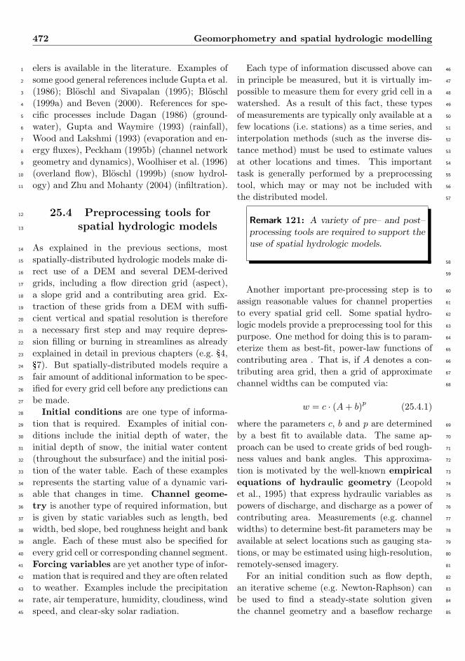
Remark 121: A variety of pre– and post–

processing tools are required to support the

use of spatial hydrologic models.

58

59

Another important pre-processing step is to 60

assign reasonable values for channel properties 61

to every spatial grid cell. Some spatial hydro- 62

logic models provide a preprocessing tool for this 63

purpose. One method for doing this is to param- 64

eterize them as best-fit, power-law functions of 65

contributing area . That is, if A denotes a con- 66

tributing area grid, then a grid of approximate 67

channel widths can be computed via: 68

w = c · (A+ b)p (25.4.1)

where the parameters c, b and p are determined 69

by a best fit to available data. The same ap- 70

proach can be used to create grids of bed rough- 71

ness values and bank angles. This approxima- 72

tion is motivated by the well-known empirical 73

equations of hydraulic geometry (Leopold 74

et al., 1995) that express hydraulic variables as 75

powers of discharge, and discharge as a power of 76

contributing area. Measurements (e.g. channel 77

widths) to determine best-fit parameters may be 78

available at select locations such as gauging sta- 79

tions, or may be estimated using high-resolution, 80

remotely-sensed imagery. 81

For an initial condition such as flow depth, 82

an iterative scheme (e.g. Newton-Raphson) can 83

be used to find a steady-state solution given 84

the channel geometry and a baseflow recharge 85

25.5 Case Study: hydrologic response of north basin, Baranja Hill 473

rate; this normal flow condition provides a rea-1

sonable initial condition. Alternately, a spatial2

model may be “spun up” from an initial state3

where flow depths are zero everywhere and run4

until a steady-state baseflow is achieved. Sim-5

ilar approaches could be used to estimate the6

initial position of the water table. Methods for7

estimating water table height based on wetness8

indices have also been proposed (see §7.6, §8.4.29

and Beven (2000)). Any of these approaches may10

be implemented as a preprocessing tool.11

When energy balance methods are used to12

model snowmelt or evapotranspiration, it is nec-13

essary to compute the net amount of shortwave14

and longwave radiation that is received by each15

grid cell. As part of this calculation one needs16

to compute the clear-sky solar radiation as a17

grid stack indexed by time. The concepts behind18

computing clear-sky radiation are discussed in19

§8.3.1 and are also reviewed by Dingman (2002,20

Appendix E). The calculation uses celestial me-21

chanics to compute the declination and zenith22

angle of the sun, as well as the times of local23

sunrise and sunset. It also takes the slope and as-24

pect of the terrain into account (as grids), along25

with several additional variables such as surface26

albedo, humidity, dustiness, cloudiness and opti-27

cal air mass. A general approach models direct,28

diffuse and backscattered radiation.29

Another useful type of preprocessing tool is30

a rainfall simulator. One method for simulating31

space-time rainfall uses the mathematics of mul-32

tifractal cascades (Over and Gupta, 1996) and33

reproduces many of the space-time scaling prop-34

erties of convective rainfall.35

It should be noted that DEMs with a vertical36

resolution of one meter do not permit a suffi-37

ciently accurate measurement of channel slope38

using the standard, local methods of geomor-39

phometry. Channel slopes are often between40

10−2 and 10−5, but for a DEM with vertical and41

horizontal resolutions of 1 and 10 meters, respec-42

tively, the minimum resolvable (nonzero) slope is43

0.1. The author has developed an experimental44

“profile-smoothing” algorithm for addressing this45

issue that is available as a preprocessing tool in46

the TopoFlow model.47

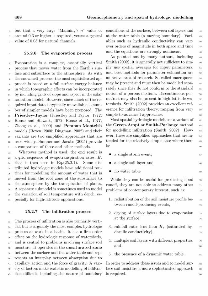
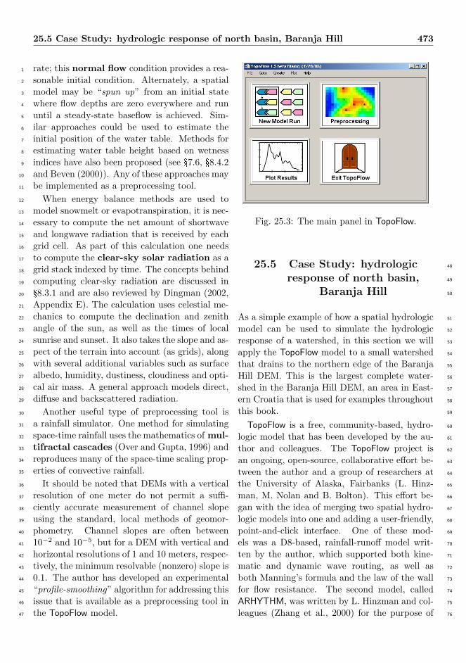
Fig. 25.3: The main panel in TopoFlow.

25.5 Case Study: hydrologic 48

response of north basin, 49

Baranja Hill 50

As a simple example of how a spatial hydrologic 51

model can be used to simulate the hydrologic 52

response of a watershed, in this section we will 53

apply the TopoFlow model to a small watershed 54

that drains to the northern edge of the Baranja 55

Hill DEM. This is the largest complete water- 56

shed in the Baranja Hill DEM, an area in East- 57

ern Croatia that is used for examples throughout 58

this book. 59

TopoFlow is a free, community-based, hydro- 60

logic model that has been developed by the au- 61

thor and colleagues. The TopoFlow project is 62

an ongoing, open-source, collaborative effort be- 63

tween the author and a group of researchers at 64

the University of Alaska, Fairbanks (L. Hinz- 65

man, M. Nolan and B. Bolton). This effort be- 66

gan with the idea of merging two spatial hydro- 67

logic models into one and adding a user-friendly, 68

point-and-click interface. One of these mod- 69

els was a D8-based, rainfall-runoff model writ- 70

ten by the author, which supported both kine- 71

matic and dynamic wave routing, as well as 72

both Manning’s formula and the law of the wall 73

for flow resistance. The second model, called 74

ARHYTHM, was written by L. Hinzman and col- 75

leagues (Zhang et al., 2000) for the purpose of 76


modelling Arctic watersheds; it therefore con-1

tained advanced methods for modelling ther-2

mal processes such as snowmelt, evaporation and3

shallow-subsurface flow. In addition to its graph-4

ical user interface, TopoFlow now provides sev-5

eral different methods for modelling infiltration6

(from Green-Ampt to the 1D Richards’ equa-7

tion) and also has a rich set of preprocessing8

tools (Fig. 25.3). Examples of such tools include9

a rainfall simulator, a data interpolation tool, a10

channel property assignment tool and a clear-sky11

solar radiation calculator.12

Before starting TopoFlow, RiverTools 3.0 (see13

§18) was used to clip a small DEM from the14

Baranja Hill DEM that contained just the north15

basin. This DEM had only 73 columns and 7616

rows, but the same grid spacing of 25 meters.17

It had minimum and maximum elevations of 8518

and 243 meters, respectively. RiverTools 3.0 was19

then used to extract several D8-based grids, in-20

cluding a flow direction grid, a slope grid, a flow21

distance grid and a contributing area grid. The22

drainage network above a selected outlet pixel23

(near the village of Popovac) was also extracted24

and had a contributing area of 1.84 square kilo-25

meters and a fairly large main-channel slope of26

0.04 [m/m]. RiverTools automatically performs27

pit-filling when necessary (see §7) but this was28

not much of an issue for this DEM because of its29

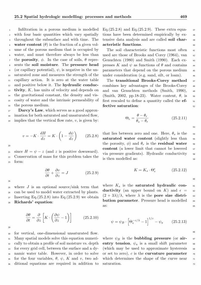
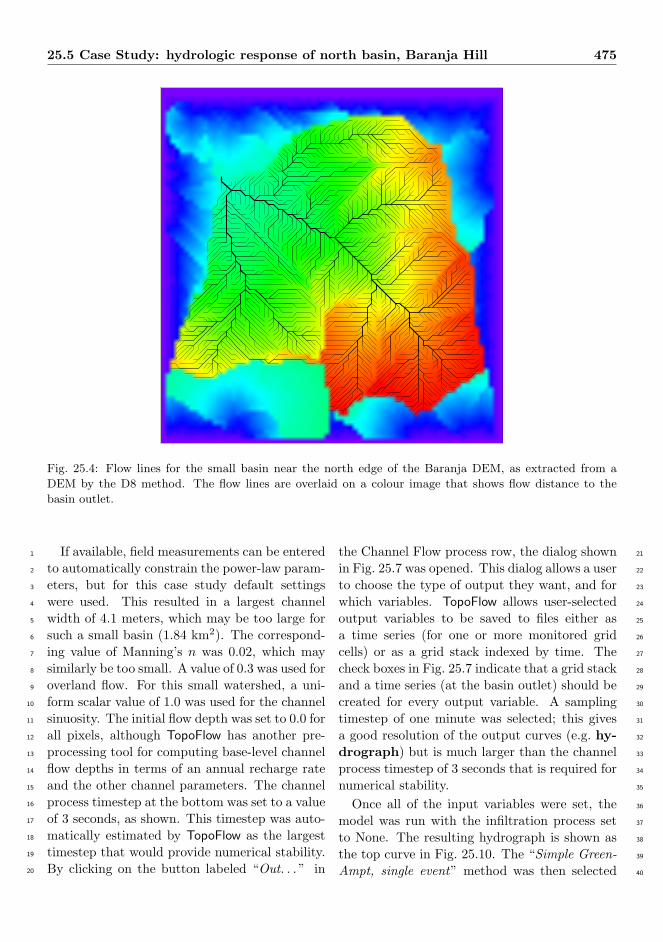
relatively steep slopes. Fig. 25.4 shows the D830

flow lines for this small watershed, overlaid on31

a grid that shows the flow distance to the edge32

of the bounding rectangle with a rainbow colour33

scheme.34

The TopoFlow model was then started as35

a plug-in from within RiverTools 3.0. It can36

also be started as a stand-alone application us-37

ing the IDL Virtual Machine, a free tool that38

can be downloaded from ITT Visual Informa-39

tion Solutions (http://www.ittvis.com/idl/).40

Fig. 25.5 shows the wizard panel in TopoFlow41

that is used to select which physical processes to42

model and which method to use for each process.43

Several methods are provided for modelling each44

hydrologic process, including both simple (e.g.45

degree-day, kinematic wave) and sophisticated46

(e.g. energy balance, dynamic wave) methods.47

In this example, spatially uniform rainfall with 48

a rate of 100 [mm/hr] and a duration of 4 min- 49

utes was selected for the Precipitation process, 50

but gridded rainfall for a fixed duration or space- 51

time rainfall as a grid stack of rainrates and a 1D 52

array of durations could have been used. For the 53

channel flow process, the kinematic wave method 54

with Manning’s formula for computing the flow 55

velocity was selected. Clicking on the button la- 56

beled “In. . . ” in the Channel Flow process row 57

opened the dialog shown in Fig. 25.6. 58

Fig. 25.5: A dialog in the TopoFlow model that al-

lows a user to select which method to use (if any)

to model each hydrologic process from a droplist of

choices. Once a choice has been selected, clicking on

the “In. . .” or “Out. . .” buttons opens an additional

dialog for entering the parameters required by that

method. Clicking on the “Eqns. . .” button displays

the set of equations that define the selected method.

All of the input dialogs in TopoFlow follow this 59

same basic template; either a scalar value can be 60

entered in the text box or the name of a file that 61

contains a time series, grid or grid sequence. The 62

filenames of the previously extracted D8-based 63

grids for flow direction and slope (from River- 64

Tools) were entered into the top two rows of this 65

dialog. The filenames for Manning’s n, channel 66

bed width and channel bank angle as grids were 67

entered in the next three rows. These were cre- 68

ated with a preprocessing tool in TopoFlow’s Cre- 69

ate menu that uses a contributing area grid and 70

power-law formulas to parameterize these quan- 71

tities. 72

25.5 Case Study: hydrologic response of north basin, Baranja Hill 475

Fig. 25.4: Flow lines for the small basin near the north edge of the Baranja DEM, as extracted from a

DEM by the D8 method. The flow lines are overlaid on a colour image that shows flow distance to the

basin outlet.

If available, field measurements can be entered1

to automatically constrain the power-law param-2

eters, but for this case study default settings3

were used. This resulted in a largest channel4

width of 4.1 meters, which may be too large for5

such a small basin (1.84 km2). The correspond-6

ing value of Manning’s n was 0.02, which may7

similarly be too small. A value of 0.3 was used for8

overland flow. For this small watershed, a uni-9

form scalar value of 1.0 was used for the channel10

sinuosity. The initial flow depth was set to 0.0 for11

all pixels, although TopoFlow has another pre-12

processing tool for computing base-level channel13

flow depths in terms of an annual recharge rate14

and the other channel parameters. The channel15

process timestep at the bottom was set to a value16

of 3 seconds, as shown. This timestep was auto-17

matically estimated by TopoFlow as the largest18

timestep that would provide numerical stability.19

By clicking on the button labeled “Out. . . ” in20

the Channel Flow process row, the dialog shown 21

in Fig. 25.7 was opened. This dialog allows a user 22

to choose the type of output they want, and for 23

which variables. TopoFlow allows user-selected 24

output variables to be saved to files either as 25

a time series (for one or more monitored grid 26

cells) or as a grid stack indexed by time. The 27

check boxes in Fig. 25.7 indicate that a grid stack 28

and a time series (at the basin outlet) should be 29

created for every output variable. A sampling 30

timestep of one minute was selected; this gives 31

a good resolution of the output curves (e.g. hy- 32

drograph) but is much larger than the channel 33

process timestep of 3 seconds that is required for 34

numerical stability. 35

Once all of the input variables were set, the 36

model was run with the infiltration process set 37

to None. The resulting hydrograph is shown as 38

the top curve in Fig. 25.10. The “Simple Green- 39

Ampt, single event” method was then selected 40


Fig. 25.9: The Display → Grid Sequence dialog in RiverTools 3.0 can be used to view grid stacks as

animations or to view/query individual frames. The frame on the left is early in a simulation, and shows

flood pulses starting to converge. The frame on the right shows the spatial pattern of discharge well into

the storm.

from the droplist of available infiltration process1

methods. Clicking on the button labeled “In. . . ”2

in the infiltration process row opened the dialog3

shown in Fig. 25.8. Toward the bottom of this4

dialog, “Clay loam” was selected as the closest5

standard soil type and the default input variables6

in the dialog were updated to ones typical of this7

soil type. The initial value of the soil moisture,8

shown as theta i was changed from the default9

of 0.1 to the value 0.35. The infiltration process10

timestep listed toward the bottom of the dialog11

was changed to 3.0 seconds per timestep, in order12

to match3 the time-step of the channel flow pro-13

cess. When the model was run again with these14

settings, it produced the hydrograph shown as15

the bottom curve in Fig. 25.10. It can be seen16

that, as expected, the inclusion of infiltration17

resulted in a much smaller peak in the hydro-18

graph and also caused the peak to occur some-19

what later. At the end of a model run, any saved20

3It can often be set to a much larger value (minutesto hours).

time series, such as a hydrograph, can be plotted 21

with the Plot → Function option. Similarly, any 22

grid stack can be visualized as a colour anima- 23

tion with the Plot → RTS File option. The RTS 24

(RiverTools Sequence) file format is a simple and 25

efficient format for storing a grid stack of data. 26

RTS files may be used to store input data, such 27

as space-time rainfall, or output data, such as 28

space-time discharge or water depth. RiverTools 29

3.0 (see §18) has similar but more powerful visu- 30

alization and query tools, including the Display 31

→ Function tool for functions (e.g. hydrographs 32

and profiles), and the Display → Grid Sequence 33

tool for grid stacks (see Fig. 25.9). The latter 34

tool allows grid stacks to be viewed frame by 35

frame or saved as AVI movie files. It also has 36

several interactive tools such as (1) a Time Pro- 37

file tool for instantly extracting a time series of 38

values for any user-selected grid cell and (2) an 39

Animated Profile tool for plotting the movement 40

of flood waves along user-selected channels. 41

It is important to realise that TopoFlow can 42

25.6 Summary points 477

Fig. 25.6: The TopoFlow dialog used to enter re-

quired input variables for the “Kinematic Wave,

Manning’s n” method of modelling channel flow.

Notice that the data type (scalar, time series, grid

or grid sequence) of each variable can be selected

from a droplist. If the data type is “Grid”, then a

filename is typed into the text box. These names

refer to grids that were created with preprocessing

tools. Units are always shown at the right edge of

the dialog.

perform much more complex simulations with-1

out much additional effort at run time. It allows2

virtually any input variable to any process to be3

entered as either a scalar (constant in space and4

time), a time series (constant in space, variable5

in time), a grid (variable in space, constant in6

time) or a grid stack (variable in space and time).7

It can also handle much larger grids than the one8

used in this case study. Advanced programming9

strategies including pointers, C-like structures,10

dynamic data typing and efficient I/O are used11

throughout TopoFlow for optimal performance12

and the ability to handle large data sets.13

25.6 Summary points14

Spatially-distributed hydrologic models make di-15

rect use of many geomorphometric variables.16

Flow direction or aspect is used to determine17

connectivity, or how water moves between neigh-18

bouring grid cells, and this same flow direction19

Fig. 25.7: The TopoFlow dialog used to choose how

model output for the channel flow process is to be

saved to files. Any output variable can be saved as

either a time series for all monitored grid cells (in

a multi-column text file) or as a sequence of grids.

The time between saved values can be specified in-

dependently of the modelling timesteps.

is also commonly used for subsurface flow. Slope 20

is one of the key variables needed to compute 21

flow velocity for both overland and channelised 22

flow. Both slope and aspect are used to compute 23

clear-sky solar radiation, which may then be used 24

by an energy-balance method to model rates 25

of snowmelt and evapotranspiration. Channel 26

lengths (between pixel centers) are used in com- 27

puting flow resistance. Elevation can be used 28

together with a lapse rate to estimate air tem- 29

perature. Total contributing area can be used to 30

determine whether overland or channelised flow 31

is dominant in a given grid cell and can also be 32

used together with scaling relationships to set 33

channel geometry variables such as bed width 34

and roughness for every grid cell. 35

One of the main advantages of spatially- 36

distributed hydrologic models over other types 37

of hydrological models is their ability to model 38

the effects of human-induced change such as land 39

use, dams, diversions, stream restoration, con- 40

taminant transport, forest fires and global warm- 41


Fig. 25.8: The TopoFlow dialog used to enter re-

quired input variables for the “Green-Ampt, sin-

gle event” method of modelling infiltration. Here,

scalars have been entered for every variable and will

be used for all grid cells. Choosing an entry from

the “Closest standard soil type” droplist changes the

input variable defaults accordingly and can be help-

ful for setting parameters when other information is

lacking. This is also useful for educational purposes.

Fig. 25.10: Two hydrographs, showing how the hy-

drologic response of the small basin differs in two

simple test cases. Both cases use spatially uniform

rainrate, but one also includes the effect of infiltra-

tion via the Green-Ampt method.

ing. A truly amazing variety of problems can1

now be addressed with fully-spatial models that2

run on a standard personal computer. While3

much work remains in order to resolve issues 4

such as upscaling, these models can be extremely 5

useful if applied with an understanding of their 6

strengths and limitations. Clearly, results do de- 7

pend on grid spacing, and the greatest uncer- 8

tainties occur when grid cells are larger than the 9

hillslope scale. For small to medium-sized basins, 10

the problem of upscaling appears to be tractable 11

and significant progress has already been made. 12

Note that many of the problems such as sub- 13

grid variability, modelling of momentum loss due 14

to friction and specification of initial conditions 15

are also encountered by fully-spatial climate and 16

ocean models. 17

Remark 122: Spatial hydrologic models

can address many types of problems that

cannot be addressed with simpler models,

such as those that involve the effects of

human-induced changes to all or part of a

watershed.

18

19

In view of the large number of distributed 20

models now used in hydrology and other fields, 21

there is clearly a growing consensus that their 22

advantages outweigh their disadvantages. A key 23

attraction of physically-based, distributed mod- 24

els is that processes are modelled with param- 25

eters that have a physical meaning; note that 26

even an effective parameter may have a well- 27

defined physical meaning. These models also 28

promote an integrated understanding of hydrol- 29

ogy, rather than focusing on a particular process 30

and neglecting others. These features combined 31

with their visual appeal makes them very effec- 32

tive educational tools, especially when a variety 33

of different methods are provided for modelling 34

different processes, when any process can easily 35

be turned off and when well-documented source 36

code is made available. 37

Important sources: 38

39

F Rivix LLC, 2004. RiverTools 3.0 User’s 40

25.6 Summary points 479

Guide. Rivix Limited Liability Company,1

Broomfield, CO, 218 pp.2

F Peckham, S.D., 2003. Fluvial landscape3

models and catchment-scale sediment trans-4

port. Global and Planetary Change, 39(1):5

31-51.6

F Bloschl, G., 2002. Scale and Scaling in Hy-7

drology — a Framework for Thinking and8

Analysis. John Wiley, Chichester, 352 pp.9

F Beven, K.J., 2000. Rainfall-Runoff Mod-10

elling: The Primer. John Wiley, New York,11

360 pp.12

F Beven, K.J., 1997. TOPMODEL: A Cri-13

tique. Hydrological Processes, 11(9): 1069-14

1086.15

chapter 25 geomorphometry and spatial hydrologic … · · 2013-08-15462 geomorphometry and...

Documents