chapter 2. graphical position velocity
DESCRIPTION
relative velocityTRANSCRIPT

7/17/2019 Chapter 2. Graphical Position Velocity ...
http://slidepdf.com/reader/full/chapter-2-graphical-position-velocity- 1/118
- 48 -
Solutions to Chapter 2 Exercise Problems
Problem 2.1
In the mechanism shown below, link 2 is rotating CCW at the rate of 2 rad/s (constant). In theposition shown, link 2 is horizontal and link 4 is vertical. Write the appropriate vector equations,solve them using vector polygons, and
a) Determine vC4, ωω ω ω 3, and ωω ω ω 4.
b) Determine aC4, αα α α 3, and αα α α 4.
Link lengths: AB = 75 mm, CD = 100 mm
B
C
2
3
4 A
D
50 mm
250 mm
ω2
Velocity Analysis:
v v v B C B C 3 3 3 3= + /
v v B B3 2=
v v v B A B A2 2 2 2= + /

7/17/2019 Chapter 2. Graphical Position Velocity ...
http://slidepdf.com/reader/full/chapter-2-graphical-position-velocity- 2/118
- 49 -
v A2 0=
Therefore,
v v v vC B C A B A3 3 3 2 2 2+ = + / / (1)
Now,
ω 2 2= rad sCCW /
v r r B A B A B A rad s mm mm s2 2 2 2 75 150 / / / ( ) ( / )( ) / = × ⊥ = =ω to
v r r C B C B C B3 3 3 / / / ( )= × ⊥ω to
v r r C D C D C D4 4 / / / ( )= × ⊥ω 44 to
Solve Eq. (1) graphically with a velocity polygon. From the polygon,
vC B mm s3 3 156 / / =
v vC D C mm s4 4 4 43 / / = =
Now,
ω 33 3 156
18286= = =
v
r
C B
C B
/
/ . rad/s
From the directions given in the position and velocity polygons
ω 3 86= . rad / s CW
Also,
ω 44 4 43
10043= = =
v
r
C D
C D
/
/ . rad/s
From the directions given in the position and velocity polygons
ω 44 = .43 rad /s CW
Acceleration Analysis:
a a a B B B A3 2 2 2= = /
a a a a aC C C D B C B3 4 4 4 3 3 3= = = + / /
a a a a a aC Dr
C Dt
B Ar
B At
C Br
C Bt
4 4 4 4 2 2 2 2 3 3 3 3 / / / / / / + = + + +(2)
Now,
a r a r B Ar
B A B Ar
B A mm2 2 2 22 2 2
2 22 75 300 / / / / = × ×( ) ⇒ = ⋅ = ⋅ =ω ω ω / s2

7/17/2019 Chapter 2. Graphical Position Velocity ...
http://slidepdf.com/reader/full/chapter-2-graphical-position-velocity- 3/118
- 50 -
in the direction of - r B A2 2/
a B At
2 20 / = since link 2 rotates at a constant speed (α 2 0= )
a r a r C Br
C B C Br
C B mm3 3 3 33 3 3
2 286 182 134 6 / / / / . .= × ×( ) ⇒ = ⋅ = ⋅ =ω ω ω / s2
in the direction of - r C B/
a r a r r C Bt
C B C Bt
C B C B3 3 3 33 3 / / / / / ( )= × ⇒ = ⋅ ⊥α α to
a r a r C Dr
C D C Dr
C D mm s4 4 4 44 4 4
2 2 243 100 18 5 / / / / . . / = × ×( ) ⇒ = ⋅ = ⋅ =ω ω ω
in the direction of - rC D/
a r a r r C Dt
C D C Dt
C D C Dto4 4 4 44 4 / / / / / ( )= × ⇒ = ⋅ ⊥α α
Solve Eq. (2) graphically with an acceleration polygon. From the acceleration polygon,
aC Bt mm s
3 319 22 / . / =
2
aC Dt mm s
4 4434 70 / . / =
2
Then,
α 33 3 67 600
2 4227 900= = =
a
r
C Bt
C B
/
/
,.
, rad/s2
α 4 4 4 434 70100 4 347= = =
a
r C D
t
C D / /
. . rad/s2
To determine the direction of αα α α 3, determine the direction that r C B/ must be rotated to be parallel to
aC Bt
3 3 / . This direction is clearly counter-clockwise.
To determine the direction of α 4, determine the direction that r C D/ must be rotated to be parallel to
aC Dt
4 4 / . This direction is clearly counter-clockwise.
From the acceleration polygon,
aC mm s4 435= / 2

7/17/2019 Chapter 2. Graphical Position Velocity ...
http://slidepdf.com/reader/full/chapter-2-graphical-position-velocity- 4/118
- 51 -
Problem 2.2
In the mechanism shown below, link 2 is rotating CCW at the rate of 500 rad/s (constant). In theposition shown, link 2 is vertical. Write the appropriate vector equations, solve them using vectorpolygons, and
a) Determinev
C4,ωω ω ω
3, andωω ω ω
4.
b) Determine aC4, αα α α 3, and αα α α 4.
Link lengths: AB = 1.2 in, BC = 2.42 in, CD = 2 in
Velocity Analysis:
v v v B C B C 3 3 3 3= + /
v v B B3 2=
v v v B A B A2 2 2 2= + /
v A2 0=
Therefore,

7/17/2019 Chapter 2. Graphical Position Velocity ...
http://slidepdf.com/reader/full/chapter-2-graphical-position-velocity- 5/118
- 52 -
v v v vC B C A B A3 3 3 2 2 2+ = + / / (1)
Now,
ω 2 500= rad s CCW /
v r r B A B A B A rad s in in s2 2 2 500 1 2 600 / / / ( ) ( / )( . ) / = × ⊥ = =ω to
v r r C B C B C B3 3 3 / / / ( )= × ⊥ω to
v r r C D C D C D4 4 / / / ( )= × ⊥ω 44 to
Solve Eq. (1) graphically with a velocity polygon. From the polygon,
vC B in s3 3 523 5 / . / =
v vC D C in s4 4 4 858 / / = =
Now,
ω 33 3 523 5
2 42216 3= = =
v
r
C B
C B
/
/
..
. rad/s
From the directions given in the position and velocity polygons
ω 3 216 3= . rad/ s CCW
Also,
ω 44 4 858
2429= = =
v
r
C D
C D
/
/ rad/s
From the directions given in the position and velocity polygons
ω 44 =429 rad s CC / W
Acceleration Analysis:
a a a B B B A3 2 2 2= = /
a a a a aC C C D B C B3 4 4 4 3 3 3= = = + / /
a a a a a aC Dr
C Dt
B Ar
B At
C Br
C Bt
4 4 4 4 2 2 2 2 3 3 3 3 / / / / / / + = + + +
(2)Now,
a r a r B Ar
B A B Ar
B A in s2 2 2 22 2 2
2 2500 1 2 300000 / / / / . / = × ×( ) ⇒ = ⋅ = ⋅ =ω ω ω 2
in the direction of - r B A2 2/
a B At
2 20 / = since link 2 rotates at a constant speed (α 2 0= )

7/17/2019 Chapter 2. Graphical Position Velocity ...
http://slidepdf.com/reader/full/chapter-2-graphical-position-velocity- 6/118
- 53 -
a r a r C Br
C B C Br
C B in3 3 3 33 3 3
2 2216 3 2 42 113 000 / / / / . . ,= × ×( ) ⇒ = ⋅ = ⋅ =ω ω ω / s2
in the direction of - r C B/
a r a r r C Bt
C B C Bt
C B C B3 3 3 33 3 / / / / / ( )= × ⇒ = ⋅ ⊥α α to
a r a r C Dr C D C Dr C D in s4 4 4 44 4 4 2 2 2429 2 368 000 / / / / , / = × ×( ) ⇒ = ⋅ = ⋅ =ω ω ω
in the direction of - rC D/
a r a r r C Dt
C D C Dt
C D C Dto4 4 4 44 4 / / / / / ( )= × ⇒ = ⋅ ⊥α α
Solve Eq. (2) graphically with an acceleration polygon. From the acceleration polygon,
aC Bt in s
3 367561 / / = 2
aC Dt in s
4 4
151437 / / =2
Then,
α 33 3 67561
2 4227 900= = =
a
r
C Bt
C B
/
/ . , rad/s2
α 44 4 151437
275 700= = =
a
r
C Dt
C D
/
/ , rad/s2
To determine the direction of αα α α 3, determine the direction that r C B/ must be rotated to be parallel to
aC Bt
3 3 / . This direction is clearly clockwise.
To determine the direction of α 4, determine the direction that r C D/ must be rotated to be parallel to
aC Dt
4 4 / . This direction is clearly clockwise.
From the acceleration polygon,
aC in s4 398 000= , / 2

7/17/2019 Chapter 2. Graphical Position Velocity ...
http://slidepdf.com/reader/full/chapter-2-graphical-position-velocity- 7/118
- 54 -
Problem 2.3
In the mechanism shown below, link 2 is rotating CW at the rate of 10 rad/s (constant). In theposition shown, link 4 is vertical. Write the appropriate vector equations, solve them using vectorpolygons, and
a) Determinev
C4,ωω ω ω
3, andωω ω ω
4.
b) Determine aC4, αα α α 3, and αα α α 4.
Link lengths: AB = 100 mm, BC = 260 mm, CD = 180 mm
B
C
2
3
4
D
250 mm
ω 2
A
Velocity Analysis:
v v v B C B C 3 3 3 3= + /
v v B B3 2=
v v v B A B A2 2 2 2= + /
v A2 0=
Therefore,
v v v vC B C A B A3 3 3 2 2 2+ = + / / (1)

7/17/2019 Chapter 2. Graphical Position Velocity ...
http://slidepdf.com/reader/full/chapter-2-graphical-position-velocity- 8/118
- 55 -
Now,
ω 2 10= rad s CW /
v r r B A B A B A rad s mm mm s2 2 2 10 100 1000 / / / ( ) ( / )( ) / = × ⊥ = =ω to
v r r C B C B C B3 3 3 / / / ( )= × ⊥ω to
v r r C D C D C D4 4 / / / ( )= × ⊥ω 44 to
Solve Eq. (1) graphically with a velocity polygon. From the polygon,
vC B mm s3 3 31 3 / . / =
v vC D C mm s4 4 4 990 / / = =
Now,
ω 33 3 31 3
260
12= = =v
r
C B
C B
/
/
. . rad/s
From the directions given in the position and velocity polygons
ω 3 12=. rad/ s CCW
Also,
ω 44 4 990
1805 5= = =
v
r
C D
C D
/
/ . rad/s
From the directions given in the position and velocity polygons
ω 44 =5 5. / rad sC W
Acceleration Analysis:
a a a B B B A3 2 2 2= = /
a a a a aC C C D B C B3 4 4 4 3 3 3= = = + / /
a a a a a aC Dr
C Dt
B Ar
B At
C Br
C Bt
4 4 4 4 2 2 2 2 3 3 3 3 / / / / / / + = + + +(2)
Now,
a r a r B Ar
B A B Ar
B A mm s2 2 2 22 2 2
2 210 100 10 000 / / / / , / = × ×( ) ⇒ = ⋅ = ⋅ =ω ω ω 2
in the direction of - r B A2 2/
a B At
2 20 / = since link 2 rotates at a constant speed (α 2 0= )
a r a r C Br
C B C Br
C B mm3 3 3 33 3 3
2 212 260 3 744 / / / / . .= × ×( ) ⇒ = ⋅ = ⋅ =ω ω ω / s2

7/17/2019 Chapter 2. Graphical Position Velocity ...
http://slidepdf.com/reader/full/chapter-2-graphical-position-velocity- 9/118
- 56 -
in the direction of - r C B/
a r a r r C Bt
C B C Bt
C B C B3 3 3 33 3 / / / / / ( )= × ⇒ = ⋅ ⊥α α to
a r a r C Dr
C D C Dr
C D mm s4 4 4 44 4 4
2 2 25 5 180 5 445 / / / / . , / = × ×( ) ⇒ = ⋅ = ⋅ =ω ω ω
in the direction of - rC D/
a r a r r C Dt
C D C Dt
C D C Dto4 4 4 44 4 / / / / / ( )= × ⇒ = ⋅ ⊥α α
Solve Eq. (2) graphically with an acceleration polygon. From the acceleration polygon,
aC Bt mm s
3 34784 / / =
2
aC Dt mm s
4 41778 / / =
2
Then,
α 33 3 4785
26018 4= = =
a
r
C Bt
C B
/
/ . rad/s2
α 44 4 1778
1809 88= = =
a
r
C Dt
C D
/
/ . rad/s2
To determine the direction of αα α α 3, determine the direction that r C B/ must be rotated to be parallel to
aC Bt
3 3 / . This direction is clearly counter-clockwise.
To determine the direction of α 4, determine the direction that r C D/ must be rotated to be parallel to
aC Dt
4 4 / . This direction is clearly counter-clockwise.
From the acceleration polygon,
aC mm s
45 700= , / 2

7/17/2019 Chapter 2. Graphical Position Velocity ...
http://slidepdf.com/reader/full/chapter-2-graphical-position-velocity- 10/118
- 57 -
Problem 2.4
In the mechanism shown below, link 2 is rotating CW at the rate of 4 rad/s (constant). In the
position shown, θ is 53˚. Write the appropriate vector equations, solve them using vector polygons,
and
a) Determine vC4, ωω ω ω 3, and ωω ω ω 4.
b) Determine aC4, αα α α 3, and αα α α 4.
Link lengths: AB = 100 mm, BC = 160 mm, CD = 200 mm
B C
2
3
4
D
ω 2 A
220 mm
160 mm
θ

7/17/2019 Chapter 2. Graphical Position Velocity ...
http://slidepdf.com/reader/full/chapter-2-graphical-position-velocity- 11/118
- 58 -
Velocity Analysis:
v v v B C B C 3 3 3 3= + /
v v B B3 2=
v v v B A B A2 2 2 2= + /
v A2 0=
Therefore,
v v v vC B C A B A3 3 3 2 2 2+ = + / / (1)
Now,
ω 2 4= rad s CW /
v r r B A B A B A rad s mm mm s2 2 2 4 100 400 / / / ( ) ( / )( ) / = × ⊥ = =ω to
v r r C B C B C B3 3 3 / / / ( )= × ⊥ω to
v r r C D C D C D4 4 / / / ( )= × ⊥ω 44 to
Solve Eq. (1) graphically with a velocity polygon. From the polygon,
vC B mm s3 3 500 / / =
v vC D C mm s4 4 4 300 / / = =
Now,
ω 33 3 500
1603 125= = =
v
r
C B
C B
/
/ . rad/s
From the directions given in the position and velocity polygons
ω 3 3 125= . rad/ s CCW
Also,
ω 44 4 300
2001 5= = =
v
r
C D
C D
/
/ . rad/s
From the directions given in the position and velocity polygons
ω 44 =1 5. / rad s CC W
Acceleration Analysis:
a a a B B B A3 2 2 2= = /
a a a a aC C C D B C B3 4 4 4 3 3 3= = = + / /
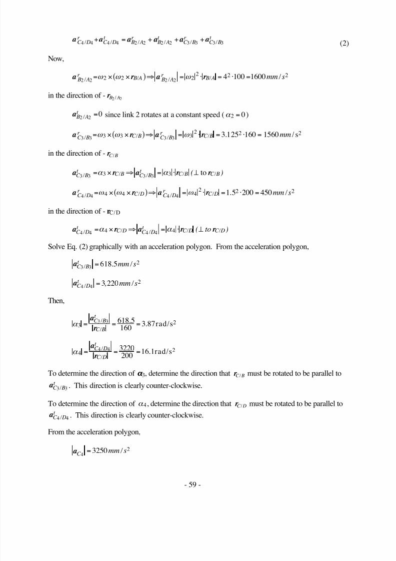
7/17/2019 Chapter 2. Graphical Position Velocity ...
http://slidepdf.com/reader/full/chapter-2-graphical-position-velocity- 12/118
- 59 -
a a a a a aC Dr
C Dt
B Ar
B At
C Br
C Bt
4 4 4 4 2 2 2 2 3 3 3 3 / / / / / / + = + + +(2)
Now,
a r a r B Ar
B A B Ar
B A mm s2 2 2 22 2 2
2 24 100 1600 / / / / / = × ×( ) ⇒ = ⋅ = ⋅ =ω ω ω 2
in the direction of -r B A2 2/
a B At
2 20 / = since link 2 rotates at a constant speed (α 2 0= )
a r a r C Br
C B C Br
C B mm3 3 3 33 3 3
2 23 125 160 1560 / / / / .= × ×( ) ⇒ = ⋅ = ⋅ =ω ω ω / s2
in the direction of - r C B/
a r a r r C Bt
C B C Bt
C B C B3 3 3 33 3 / / / / / ( )= × ⇒ = ⋅ ⊥α α to
a r a r C D
r
C D C D
r
C D mm s
4 4 4 44 4 4
2 2 2
1 5 200 450 / / / / . / = × ×( ) ⇒ = ⋅ = ⋅ =ω ω ω
in the direction of - rC D/
a r a r r C Dt
C D C Dt
C D C Dto4 4 4 44 4 / / / / / ( )= × ⇒ = ⋅ ⊥α α
Solve Eq. (2) graphically with an acceleration polygon. From the acceleration polygon,
aC Bt mm s
3 3618 5 / . / =
2
aC Dt mm s
4 43 220 / , / =
2
Then,
α 33 3 618 5
1603 87= = =
a
r
C Bt
C B
/
/
. . rad/s2
α 44 4 3220
20016 1= = =
a
r
C Dt
C D
/
/ . rad/s2
To determine the direction of αα α α 3, determine the direction that r C B/ must be rotated to be parallel to
aC Bt
3 3 / . This direction is clearly counter-clockwise.
To determine the direction of α 4, determine the direction that r C D/ must be rotated to be parallel to
aC Dt
4 4 / . This direction is clearly counter-clockwise.
From the acceleration polygon,
aC mm s
43250= / 2

7/17/2019 Chapter 2. Graphical Position Velocity ...
http://slidepdf.com/reader/full/chapter-2-graphical-position-velocity- 13/118
- 60 -
Problem 2.5
In the mechanism shown below, link 2 is rotating CCW at the rate of 4 rad/s (constant). In theposition shown, link 2 is horizontal. Write the appropriate vector equations, solve them using vectorpolygons, and
a) Determinev
C4,ωω ω ω
3, andωω ω ω
4.
b) Determine aC4, αα α α 3, and αα α α 4.
Link lengths: AB = 1.25 in, BC = 2.5 in, CD = 2.5 in
B
C
2
3
4
D
ω 2
A
1.0 in
0.75 in
Velocity Analysis:
v v v B C B C 3 3 3 3= + /
v v B B3 2=

7/17/2019 Chapter 2. Graphical Position Velocity ...
http://slidepdf.com/reader/full/chapter-2-graphical-position-velocity- 14/118
- 61 -
v v v B A B A2 2 2 2= + /
v A2 0=
Therefore,
v v v vC B C A B A3 3 3 2 2 2+ = + / / (1)
Now,
ω 2 4= rad s CCW /
v r r B A B A B A rad s in in s2 2 2 4 1 25 5 / / / ( ) ( / )( . ) / = × ⊥ = =ω to
v r r C B C B C B3 3 3 / / / ( )= × ⊥ω to
v r r C D C D C D4 4 / / / ( )= × ⊥ω 44 to
Solve Eq. (1) graphically with a velocity polygon. From the polygon,
vC B in s3 3 6 25 / . / =
v vC D C in s4 4 4 3 75 / . / = =
Now,
ω 33 3 6 25
2 52 5= = =
v
r
C B
C B
/
/
..
. rad/s
From the directions given in the position and velocity polygons
ω 3 2 5= . rad/ s CCW
Also,
ω 44 4 3 75
2 51 5= = =
v
r
C D
C D
/
/
..
. rad/s
From the directions given in the position and velocity polygons
ω 44 =1 5. / rad sC W
Acceleration Analysis:
a a a B B B A3 2 2 2= = /
a a a a aC C C D B C B3 4 4 4 3 3 3= = = + / /
a a a a a aC Dr
C Dt
B Ar
B At
C Br
C Bt
4 4 4 4 2 2 2 2 3 3 3 3 / / / / / / + = + + +(2)
Now,

7/17/2019 Chapter 2. Graphical Position Velocity ...
http://slidepdf.com/reader/full/chapter-2-graphical-position-velocity- 15/118
- 62 -
a r a r B Ar
B A B Ar
B A in s2 2 2 22 2 2
2 24 1 25 20 / / / / . / = × ×( ) ⇒ = ⋅ = ⋅ =ω ω ω 2
in the direction of - r B A2 2/
a B At
2 20 / = since link 2 rotates at a constant speed (α 2 0= )
a r a r C Br C B C Br C B in3 3 3 33 3 3 2 22 5 2 5 15 6 / / / / . . .= × ×( ) ⇒ = ⋅ = ⋅ =ω ω ω / s2
in the direction of - r C B/
a r a r r C Bt
C B C Bt
C B C B3 3 3 33 3 / / / / / ( )= × ⇒ = ⋅ ⊥α α to
a r a r C Dr
C D C Dr
C D in s4 4 4 44 4 4
2 2 21 5 2 5 5 6 / / / / . . . / = × ×( ) ⇒ = ⋅ = ⋅ =ω ω ω
in the direction of - rC D/
a r a r r C D
t
C D C D
t
C D C Dto4 4 4 44 4 / / / / / ( )= × ⇒ = ⋅ ⊥α α
Solve Eq. (2) graphically with an acceleration polygon. From the acceleration polygon,
aC Bt in s
3 34 69 / . / =
2
aC Dt in s
4 44 69 / . / =
2
Then,
α
3
3 3 4 69
2 51 87= = =
a
r
C Bt
C B
/
/
.
. . rad/s2
α 44 4 4 69
2 51 87= = =
a
r
C Dt
C D
/
/
..
. rad/s2
To determine the direction of αα α α 3, determine the direction that r C B/ must be rotated to be parallel to
aC Bt
3 3 / . This direction is clearly counter-clockwise.
To determine the direction of α 4, determine the direction that r C D/ must be rotated to be parallel to
aC Dt
4 4 / . This direction is clearly clockwise.
From the acceleration polygon,
aC in s4
7 32= . / 2

7/17/2019 Chapter 2. Graphical Position Velocity ...
http://slidepdf.com/reader/full/chapter-2-graphical-position-velocity- 16/118
- 63 -
Problem 2.6
In the mechanism shown below, link 2 is rotating CW at the rate of 100 rad/s (constant). In theposition shown, link 2 is horizontal. Write the appropriate vector equations, solve them using vectorpolygons, and
a) Determine vC4 and ωω ω ω 3
b) Determine aC4 and αα α α 3
Link lengths: AB = 60 mm, BC = 200 mm
B
C
2
3
4
ω 2
A
120 mm
Velocity Analysis:
v v v B C B C 3 3 3 3= + /
v v B B3 2=
v v v B A B A2 2 2 2= + /
v A2 0=
Therefore,
v v v vC B C A B A3 3 3 2 2 2+ = + / / (1)

7/17/2019 Chapter 2. Graphical Position Velocity ...
http://slidepdf.com/reader/full/chapter-2-graphical-position-velocity- 17/118
- 64 -
Now,
ω 2 100= rad s CW /
v r r B A B A B A rad s mm mm s2 2 2 100 60 6000 / / / ( ) ( / )( ) / = × ⊥ = =ω to
v r r C B C B C B3 3 3 / / / ( )= × ⊥ω to
vC D4 4 / → parallel to the ground.
Solve Eq. (1) graphically with a velocity polygon. From the polygon,
vC B mm s3 3 7 500 / , / =
v vC D C mm s4 4 4 4500 / / = =
Now,
ω 33 3 7500
20037 5= = =
v
r
C B
C B
/
/
. rad/s
From the directions given in the position and velocity polygons
ω 3 12=. rad / s CW
Acceleration Analysis:
a a a B B B A3 2 2 2= = /
a a a a aC C C D B C B3 4 4 4 3 3 3= = = + / /
a a a a a aC Dr C Dt B Ar B At C Br C Bt 4 4 4 4 2 2 2 2 3 3 3 3 / / / / / / + = + + + (2)
Now,
a r a r B Ar
B A B Ar
B A mm s2 2 2 22 2 2
2 2100 60 600 000 / / / / , / = × ×( ) ⇒ = ⋅ = ⋅ =ω ω ω 2
in the direction of - r B A2 2/
a B At
2 20 / = since link 2 rotates at a constant speed (α 2 0= )
a r a r C B
r
C B C B
r
C B mm3 3 3 33 3 3
2 2
37 5 200 281 000 / / / / . ,= × ×
( )⇒ = ⋅ = ⋅ =ω ω ω
/ s2
in the direction of - r C B/
a r a r r C Bt
C B C Bt
C B C B3 3 3 33 3 / / / / / ( )= × ⇒ = ⋅ ⊥α α to
a aC D C 4 4 4 / = →parallel to ground
Solve Eq. (2) graphically with an acceleration polygon. From the acceleration polygon,

7/17/2019 Chapter 2. Graphical Position Velocity ...
http://slidepdf.com/reader/full/chapter-2-graphical-position-velocity- 18/118
- 65 -
aC Bt mm s
3 3211 000 2
/ , / =
a aC D C mm s4 4 4
248 000 2 / , / = =
Then,
α 33 3 211 000
2001060= = =a
r C Bt
C B
/
/ , rad/s2
To determine the direction of αα α α 3, determine the direction that r C B/ must be rotated to be parallel to
aC Bt
3 3 / . This direction is clearly counter-clockwise.
From the acceleration polygon,
aC mm s4
248 000= , / 2
Problem 2.7
In the mechanism shown below, link 4 is moving to the left at the rate of 4 ft/s (constant). Write theappropriate vector equations, solve them using vector polygons, and
a) Determine ωω ω ω 3 and ωω ω ω 4.
b) Determine αα α α 3 and αα α α 4.
Link lengths: AB = 10 ft, BC = 20 ft.
B
C
23
4
A
8.5 ft
120˚
vC4

7/17/2019 Chapter 2. Graphical Position Velocity ...
http://slidepdf.com/reader/full/chapter-2-graphical-position-velocity- 19/118
- 66 -
Velocity Analysis:
v v v B C B C 3 3 3 3= + /
v v B B3 2=
v v v B A B A2 2 2 2= + /
v A2 0=
Therefore,
v v v vC B C A B A3 3 3 2 2 2+ = + / / (1)
Now,
vC 4 4= f t / s parallel to the ground
v r r B C B C B C 3 3 3 / / / ( )= × ⊥ω to
v r r B A B A B A2 2 2 / / / ( )= × ⊥ω to
Solve Eq. (1) graphically with a velocity polygon. From the polygon,
v B C ft s3 3 2 3 / . / =
v B A ft s2 2 2 3 / . / =
or
ω 33 3 2 3
20115= = =
v
r
B C
B C
/
/
. . rad/s
From the directions given in the position and velocity polygons

7/17/2019 Chapter 2. Graphical Position Velocity ...
http://slidepdf.com/reader/full/chapter-2-graphical-position-velocity- 20/118
- 67 -
ω 3 115=. rad / s CW
Also,
ω 22 2 2 3
1023= = =
v
r
B A
B A
/
/
. . rad/s
From the directions given in the position and velocity polygons
ω 2 23=. rad /s CCW
ω 4 0= rad / s since it does not rotate
Acceleration Analysis:
a a a a aC C C D B C B3 4 4 4 3 3 3= = = + / /
a a a a a aC Dr
C Dt
B Ar
B At
C Br
C Bt
4 4 4 4 2 2 2 2 3 3 3 3 / / / / / / + = + + + (2)
Now,
a r a r B Ar
B A B Ar
B A ft s2 2 2 22 2 2
2 223 10 529 / / / / . . / = × ×( ) ⇒ = ⋅ = ⋅ =ω ω ω 2
in the direction of - r B A2 2 /
a r a r r B At
B A B At
B A B A2 2 2 22 2 / / / / / ( )= × ⇒ = ⋅ ⊥α α to
a r a r C Br
C B C Br
C B ft 3 3 3 33 3 3
2 2115 20 264 / / / / . .= × ×( ) ⇒ = ⋅ = ⋅ =ω ω ω / s2
in the direction of - r C B /
a r a r r C Bt
C B C Bt
C B C B3 3 3 33 3 / / / / / ( )= × ⇒ = ⋅ ⊥α α to
a C D4 40 / = link 4 is moving at a constant velocity
Solve Eq. (2) graphically with an acceleration polygon. From the acceleration polygon,
aC Bt ft s
3 30 045 / . / =
2
a B At ft s
2 20 017 2
/ . / =
Then,
α 33 3 0 45
20023= = =
a
r
C Bt
C B
/
/
. . rad/s2
α 22 2 0 017
100017= = =
a
r
B At
B A
/
/
. . rad/s2

7/17/2019 Chapter 2. Graphical Position Velocity ...
http://slidepdf.com/reader/full/chapter-2-graphical-position-velocity- 21/118
- 68 -
To determine the direction of αα α α 3, determine the direction that r C B / must be rotated to be parallel to
aC Bt
3 3 / . This direction is clearly clockwise.
To determine the direction of αα α α 2, determine the direction that r B A / must be rotated to be parallel to
a B At
2 2 / . This direction is clearly counter-clockwise.
Problem 2.8
In the mechanism shown below, link 4 is moving to the right at the rate of 20 in/s (constant). Writethe appropriate vector equations, solve them using vector polygons, and
a) Determine ωω ω ω 3 and ωω ω ω 4.
b) Determine αα α α 3 and αα α α 4.
Link lengths: AB = 5 in, BC = 5 in.
2
A
B
C 3
4
7 in
45˚
vC4

7/17/2019 Chapter 2. Graphical Position Velocity ...
http://slidepdf.com/reader/full/chapter-2-graphical-position-velocity- 22/118
- 69 -
Velocity Analysis:
v v v B C B C 3 3 3 3= + /
v v B B3 2=
v v v B A B A2 2 2 2= + /
v A2 0=
Therefore,
v v v vC B C A B A3 3 3 2 2 2+ = + / / (1)
Now,
vC in s4 20= / parallel to the ground
v r r B C B C B C 3 3 3 / / / ( )= × ⊥ω to
v r r B A B A B A2 2 2 / / / ( )= × ⊥ω to
Solve Eq. (1) graphically with a velocity polygon. From the polygon,
v B C in s3 3 14 1 / . / =
v B A in s2 2 14 1 / . / =
or
ω 33 3 14 1
52 82= = =
v
r
B C
B C
/
/
. . rad/s
From the directions given in the position and velocity polygons
ω 3 2 82= . rad /s CCW
Also,
ω 22 2 14 1
52 82= = =
v
r
B A
B A
/
/
. . rad/s
From the directions given in the position and velocity polygons
ω 2 2 82= . rad /s CCW
ω 4 0= rad / s since it doesn’t rotate
Acceleration Analysis:
a a a B B B A3 2 2 2= = /
a a a a aC C C D B C B3 4 4 4 3 3 3= = = + / /

7/17/2019 Chapter 2. Graphical Position Velocity ...
http://slidepdf.com/reader/full/chapter-2-graphical-position-velocity- 23/118
- 70 -
a a a a a aC Dr
C Dt
B Ar
B At
C Br
C Bt
4 4 4 4 2 2 2 2 3 3 3 3 / / / / / / + = + + +(2)
Now,
a r a r B Ar
B A B Ar
B A in s2 2 2 22 2 2
2 22 82 5 39 8 / / / / . . / = × ×( ) ⇒ = ⋅ = ⋅ =ω ω ω 2
in the direction of - r B A2 2/
a r a r r B At
B A B At
B A B A2 2 2 22 2 / / / / / ( )= × ⇒ = ⋅ ⊥α α to
a r a r C Br
C B C Br
C B in3 3 3 33 3 3
2 22 82 5 39 8 / / / / . .= × ×( ) ⇒ = ⋅ = ⋅ =ω ω ω / s2
in the direction of - r C B/
a r a r r C Bt
C B C Bt
C B C B3 3 3 33 3 / / / / / ( )= × ⇒ = ⋅ ⊥α α to
aC D4 4 0 /
=
link 4 is moving at a constant velocity
Solve Eq. (2) graphically with an acceleration polygon. From the acceleration polygon,
aC Bt in s
3 338 8 / . / =
2
a B At in s
2 238 8 2
/ . / =
Then,
α 33 3 38 8
57 76= = =
a
r
C Bt
C B
/
/
. . rad/s2
α 22 2 38 8
57 76= = =
a
r
B At
B A
/
/
. . rad/s2
α 4 0 4= ( )link isnotrotating
To determine the direction of αα α α 3, determine the direction that r C B/ must be rotated to be parallel to
aC Bt
3 3 / . This direction is clearly counter-clockwise.
To determine the direction of α 22 , determine the direction that r B A / must be rotated to be parallel to
a B At
2 2 / . This direction is clearly clockwise.

7/17/2019 Chapter 2. Graphical Position Velocity ...
http://slidepdf.com/reader/full/chapter-2-graphical-position-velocity- 24/118
- 71 -
Problem 2.9
In the mechanism shown below, link 4 is moving to the left at the rate of 0.6 ft/s (constant). Writethe appropriate vector equations, solve them using vector polygons, and determine the velocity andacceleration of point A3.
Link lengths: AB = 5 in, BC = 5 in.
2
A
B
C
3
4 vC4
135˚
Velocity Analysis:
v v v B C B C 3 3 3 3= + /
v v B B3 2=
v v v B A B A3 3 3 3= + /
Therefore,
v v v vC B C A B A3 3 3 3 3 3+ = + / / (1)

7/17/2019 Chapter 2. Graphical Position Velocity ...
http://slidepdf.com/reader/full/chapter-2-graphical-position-velocity- 25/118
- 72 -
Now,
vC 4 6= . f t / sparallel to the ground
v r r B C B C B C 3 3 3 / / / ( )= × ⊥ω to
v r r B A B A B A3 3 3 / / / ( )= × ⊥ω to
Solve Eq. (1) graphically with a velocity polygon. From the polygon,
v B C ft s3 3 85 / . / =
or
ω 33 3 85
5 122 04= = =
v
r
B C
B C
/
/
.( / )
. rad/s
From the directions given in the position and velocity polygons
ω 3 2 04
=
. rad / s CW
Now,
v r r B A B A B A ft s3 3 3 2 04 5 12 85 / / / ( ) ( . )( / ) . / = × ⊥ = =ω to
Using velocity image,
v A ft s3 1 34= . /
Acceleration Analysis:
a aC C 4 3
0= =
a a a a a B B B C r
B C t
B C 3 2 3 3 3 3 3 3= = = + / / / (2)
Now,
a r a r B C r
B C B C r
B C ft s3 3 3 33 3 3
2 22 04 5 12 1 73 / / / / . ( / ) . / = × ×( ) ⇒ = ⋅ = ⋅ =ω ω ω 2
in the direction of - r B C 3 3 /
a r a r r B C t
B C B C t
B C B C 3 3 3 3 3 / / / / / ( )= × ⇒ = ⋅ ⊥α α 33 to
a C D4 40 / = link 4 is moving at a constant velocity
Solve Eq. (2) graphically with an acceleration polygon. From the acceleration polygon,
a B C t ft s
3 31 73 / . / =
2
Then,

7/17/2019 Chapter 2. Graphical Position Velocity ...
http://slidepdf.com/reader/full/chapter-2-graphical-position-velocity- 26/118
- 73 -
α 33 3 1 73
5 124 15= = =
a
r
B C t
B C
/
/
.( / )
. rad/s2
To determine the direction of αα α α 3, determine the direction that r B C / must be rotated to be parallel to
a B C t
3 3 / . This direction is clearly clockwise.
Using acceleration image,
a A ft s3
4 93= . / 2
Problem 2.10
In the mechanism shown below, link 4 moves to the right with a constant velocity of 75 ft/s. Writethe appropriate vector equations, solve them using vector polygons, and
a) Determine vB2, vG3, ωω ω ω 2, and ωω ω ω 3.
b) Determine aB2, aG3, αα α α 2, and αα α α 3.
Link lengths: AB in= 4 8. , BC in= 16 0. , BG in= 6 0.
A
B
C
G
2 3
442˚
Position Analysis: Draw the linkage to scale.

7/17/2019 Chapter 2. Graphical Position Velocity ...
http://slidepdf.com/reader/full/chapter-2-graphical-position-velocity- 27/118
- 74 -
B
G
2 3
42˚
A C
AB = 4.8"BC = 16.0"BG = 6.0"AC = 19.33"
g3
a1 a 2,
ovc3 c4,
b2 b3,
25 ft/sec
Velocity Polygon
Velocity Analysis:
v v v B C B C 3 3 3 3= + /
v v B B3 2=

7/17/2019 Chapter 2. Graphical Position Velocity ...
http://slidepdf.com/reader/full/chapter-2-graphical-position-velocity- 28/118
- 75 -
v v v B A B A2 2 2 2= + /
v A2 0=
Therefore,
v v v vC B C A B A3 3 3 2 2 2+ = + / / (1)
Now,
vC 3 75= f t / sin the direction of r C A/
v r r B C B C B C 3 3 3 / / / ( )= × ⊥ω to
v r r B A B A B A2 2 2 / / / ( )= × ⊥ω to
Solve Eq. (1) graphically with a velocity polygon. From the polygon,
v B C ft s3 3 69 4 / . / =
or
ω 33 3 69 4
16 1 1252= = =
v
r
B C
B C
/
/
.( / )
rad/s
From the directions given in the position and velocity polygons
ω 3 52= rad/ s CCW
Also,
ω 22 2 91 5
4 8 1 12228= = =v
r
B A
B A
/
/
.. ( / )
rad/s
From the directions given in the position and velocity polygons
ω 2 228= rad /s CW
To compute the velocity of G3,
v v v v r G B G B B G B3 3 3 3 3 3 33= + = + × / / ω
Using the values computed previously
ω 3 3 3 52 6 0 312× = =r G B / ( . ) in/s
and from the directions given in the velocity and position diagrams
ω 3 3 3 3 3312× = ⊥r r G B G B / / in/s
Now draw vG3 on the velocity diagram
vG3 79 0= . f t / s in the direction shown.

7/17/2019 Chapter 2. Graphical Position Velocity ...
http://slidepdf.com/reader/full/chapter-2-graphical-position-velocity- 29/118
- 76 -
Acceleration Analysis:
a a a B B B A3 2 2 2= = /
a a a a aC C C D B C B3 4 4 4 3 3 3= = = + / /
a a a a a aC Dr
C Dt
B Ar
B At
C Br
C Bt
4 4 4 4 2 2 2 2 3 3 3 3 / / / / / / + = + + +(2)
Now,
a r a r B Ar
B A B Ar
B A ft s2 2 2 22 2 2
2 2228 4 8 12 20 900 / / / / ( . / ) , / = × ×( ) ⇒ = ⋅ = ⋅ =ω ω ω 2
in the direction of - r B A2 2/
a r a r r B At
B A B At
B A B A2 2 2 22 2 / / / / / ( )= × ⇒ = ⋅ ⊥α α to
a r a r C Br
C B C Br
C B ft 3 3 3 33 3 3
2 252 16 12 3605 / / / / ( / )= × ×( ) ⇒ = ⋅ = ⋅ =ω ω ω / s2
in the direction of - r C B/
a r a r r C Bt
C B C Bt
C B C B3 3 3 33 3 / / / / / ( )= × ⇒ = ⋅ ⊥α α to
a C D4 40 / = link 4 is moving at a constant velocity
Solve Eq. (2) graphically with an acceleration polygon. From the acceleration polygon,
aC Bt ft s
3 328 700 / , / =
2
a B At ft s
2 2
20 000 2 / , / =
Then,
α 33 3 28 700
16 1221 500= = =
a
r
C Bt
C B
/
/
,( / )
, rad/s2
α 22 2 20 000
4 8 1250 000= = =
a
r
B At
B A
/
/
,( . / )
, rad/s2
To determine the direction of α 3 , determine the direction that r C B/ must be rotated to be parallel to
aC Bt
3 3 / . This direction is clearly clockwise.
To determine the direction of α 22 , determine the direction that r B A / must be rotated to be parallel to
a B C t
2 2 / . This direction is clearly counter-clockwise.
From the acceleration polygon,
a B ft s
228 900= , / 2

7/17/2019 Chapter 2. Graphical Position Velocity ...
http://slidepdf.com/reader/full/chapter-2-graphical-position-velocity- 30/118
- 77 -
To compute the acceleration of G3, use acceleration image. From the acceleration polygon,
aG ft s3
18 000= , / 2
Problem 2.11
For the four-bar linkage, assume that ωω ω ω 2 = 50 rad/s CW and αα α α 2 = 1600 rad/s2 CW. Write the
appropriate vector equations, solve them using vector polygons, and
a) Determine vB2, vC3, vE3
, ωω ω ω 3, and ωω ω ω 4.
b) Determine aB2, aC3, aE3
,αα α α 3, and αα α α 4.
B
E
A D
C
2
3
4
120˚
AB = 1.75" AD = 3.55"CD = 2.75" BC = 5.15" BE = 2.5" EC = 4.0"
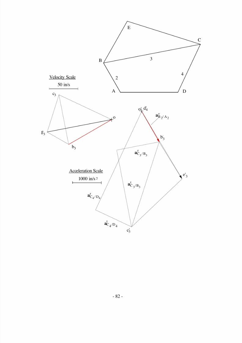
Position Analysis
Draw the linkage to scale. Start by locating the relative positions of A and D. Next locate B andthen C. Then locate E.
Velocity Analysis:
v v v B B B A3 2 2 2= = /
v v v v vC C C D B C B3 4 4 4 3 3 3= = = + / / (1)
Now,
v r v r r B A B A B A B A B A2 2 2 2 50 1 75 87 5 / / / / / . . ( )= × ⇒ = ⋅ = ⋅ = ⊥ω ω in / s to
v r v r r C D C D C D C D C D4 4 4 44 4 / / / / / ( )= × ⇒ = ⋅ ⊥ω ω to
v r v r r C B C B C B C B C B3 3 3 33 3 / / / / / ( )= × ⇒ = ⋅ ⊥ω ω to

7/17/2019 Chapter 2. Graphical Position Velocity ...
http://slidepdf.com/reader/full/chapter-2-graphical-position-velocity- 31/118
- 78 -
3 3aC / B
t
aC3 / B3
r
aC4 /D4
t
aC 4 /D 4
r
c'3
b'3
o' d'4
C
B
D
2
3
4
A
E
50 in/s
Velocity Scale
b3
o
c3
e3
2000 in/s
Acceleration Scale
2
aB 2 /A2
t
aB2 / A2
r
e'3
Solve Eq. (1) graphically with a velocity polygon and locate the velocity of point E3 by image.From the polygon,
vC B3 3 65 2 / .= in/s
vC D4 4 92 6 / .= in /s
and
v E 3 107 8= . in/s
in the direction shown.
Now
ω 33 3 65 2
5 1512 7= = =
v
r
C B
C B
/
/
..
. rad/s

7/17/2019 Chapter 2. Graphical Position Velocity ...
http://slidepdf.com/reader/full/chapter-2-graphical-position-velocity- 32/118
- 79 -
and
ω 44 4 92 6
2 7533 7= = =
v
r
C D
C D
/
/
..
. rad/s
To determine the direction of ω 3, determine the direction that r C B/ must be rotated to be parallel to
vC B3 3 / . This direction is clearly clockwise.
To determine the direction of ω 4 , determine the direction that r C D/ must be rotated to be parallel to
vC D4 4 / . This direction is clearly clockwise.
Acceleration Analysis:
a a a B B B A3 2 2 2= = /
a a a a aC C C D B C B3 4 4 4 3 3 3= = = + / /
a a a a a aC Dr
C Dt
B Ar
B At
C Br
C Bt
4 4 4 4 2 2 2 2 3 3 3 3 / / / / / / + = + + +(2)
Now,
a r a r B Ar
B A B Ar
B A2 2 2 22 2 22 250 1 75 4375 / / / / .= × ×( ) ⇒ = ⋅ = ⋅ =ω ω ω in /s2
in the direction of - r B A2 2/
a r a r r B At
B A B At
B A B A2 2 2 22 2 1600 1 75 2800 / / / / / . ( )= × ⇒ = = ⋅ = ⊥α α in / s to2
a r a r C Br
C B C Br
C B3 3 3 33 3 32 212 7 5 15 830 6 / / / / . . .= × ×( ) ⇒ = ⋅ = ⋅ =ω ω ω in/s2
in the direction of - r C B/
a r a r r C Bt
C B C Bt
C B C B3 3 3 33 3 / / / / / ( )= × ⇒ = ⋅ ⊥α α to
a r a r C Dr
C D C Dr
C D in4 4 4 44 4 4
2 2 233 7 2 75 3123 / / / / . . / sec= × ×( ) ⇒ = ⋅ = ⋅ =ω ω ω
in the direction of - rC D/
a r a r r C Dt
C D C Dt
C D C Dto4 4 4 44 4 / / / / / ( )= × ⇒ = ⋅ ⊥α α
Solve Eq. (2) graphically with an acceleration polygon and determine the acceleration of point E3 byimage. From the acceleration polygon,
aC Bt
3 31563 / = in/s2
aC Dt
4 44881 / = in/s2
Then,

7/17/2019 Chapter 2. Graphical Position Velocity ...
http://slidepdf.com/reader/full/chapter-2-graphical-position-velocity- 33/118
- 80 -
α 33 3 1563
5 15303= = =
a
r
C Bt
C B
/
/ .rad/s2
α 44 4 4881
2 751775= = =
a
r
C Dt
C D
/
/ .rad/s2
To determine the direction ofα
3 , determine the direction thatr C B/ must be rotated to be parallel to
aC Bt
3 3 / . This direction is clearly clockwise.
To determine the direction of α 4, determine the direction that r C D/ must be rotated to be parallel to
aC Dt
4 4 / . This direction is clearly clockwise.
Also
a E 3 5958= in/s2
Problem 2.12
Resolve Problem 2.11 if ωω ω ω 2 = 50 rad/s CCW and αα α α 2 = 0 .
Position Analysis
Draw the linkage to scale. Start by locating the relative positions of A and D. Next locate B andthen C. Then locate E.
Velocity Analysis:
The velocity analysis is similar to that in Problem 2.18.
v v v B B B A3 2 2 2= = /
v v v v vC C C D B C B3 4 4 4 3 3 3= = = + / / (1)
Now,
v r v r r B A B A B A B A B A2 2 2 2 50 1 75 87 5 / / / / / . . ( )= × ⇒ = ⋅ = ⋅ = ⊥ω ω in / s to
v r v r r C D C D C D C D C D4 4 4 44 4 / / / / / ( )= × ⇒ = ⋅ ⊥ω ω to
v r v r r C B C B C B C B C B3 3 3 33 3 / / / / / ( )= × ⇒ = ⋅ ⊥ω ω to
Solve Eq. (1) graphically with a velocity polygon and locate the velocity of point E3 by image.From the polygon,
vC D4 4 103 1 / .= in/s
and
v E 3 116= in/s

7/17/2019 Chapter 2. Graphical Position Velocity ...
http://slidepdf.com/reader/full/chapter-2-graphical-position-velocity- 34/118
- 81 -
in the direction shown.
Now
ω 33 3 88 8
5 1517 2= = =
v
r
C B
C B
/
/
..
. rad/s
and
ω 44 4 103 1
2 7537 5= = =
v
r
C D
C D
/
/
..
. rad/s
To determine the direction of ω 3, determine the direction that r C B/ must be rotated to be parallel to
vC B3 3 / . This direction is clearly counterclockwise.
To determine the direction of ω 4 , determine the direction that r C D/ must be rotated to be parallel to
vC D4 4 / . This direction is clearly counterclockwise.
7/17/2019 Chapter 2. Graphical Position Velocity ...
http://slidepdf.com/reader/full/chapter-2-graphical-position-velocity- 35/118
- 82 -
3 3aC /B
t
aC3
/ B3
r
aC4 /D4
t
aC4 / D4
r
c'3
b'3
o' d'4
C
B
D
2
3
4
A
E
50 in/s
Velocity Scale
c3
b3
o
g3
1000 in/s
Acceleration Scale
2
aB 2/ A2
r
e'3

7/17/2019 Chapter 2. Graphical Position Velocity ...
http://slidepdf.com/reader/full/chapter-2-graphical-position-velocity- 36/118
- 83 -
Acceleration Analysis:
a a a B B B A3 2 2 2= = /
a a a a aC C C D B C B3 4 4 4 3 3 3= = = + / /
a a a a a aC Dr
C Dt
B Ar
B At
C Br
C Bt
4 4 4 4 2 2 2 2 3 3 3 3 / / / / / / + = + + + (2)
Now,
a r a r B Ar
B A B Ar
B A2 2 2 22 2 22 250 1 75 4375 / / / / .= × ×( ) ⇒ = ⋅ = ⋅ =ω ω ω in /s2
in the direction of - r B A2 2/
a r a r B At
B A B At
B A2 2 2 22 2 0 1 75 0 / / / / .= × ⇒ = = ⋅ =α α
a r a r C Br
C B C Br
C B3 3 3 3
3 3 32 217 24 5 15 1530 / / / / . .= × ×( ) ⇒ = ⋅ = ⋅ =ω ω ω in/s2
in the direction of - r C B/
a r a r r C Bt
C B C Bt
C B C B3 3 3 33 3 / / / / / ( )= × ⇒ = ⋅ ⊥α α to
a r a r C Dr
C D C Dr
C D4 4 4 44 4 42 237 49 2 75 3865 / / / / . .= × ×( ) ⇒ = ⋅ = ⋅ =ω ω ω in/s2
in the direction of - rC D/
a r a r r C Dt
C D C Dt
C D C Dto4 4 4 44 4 / / / / / ( )= × ⇒ = ⋅ ⊥α α
Solve Eq. (2) graphically with an acceleration polygon and determine the acceleration of point E3 byimage. From the acceleration polygon,
a
a
C Bt
C Dt
3 3
4 4
2751
1405
/
/
=
=
in/s
in/s
2
2
Then,
α
α
32
4
3 3
4 4
27515 15
534
14052 75
511
= = =
= = =
a
r
a
r
C Bt
C B
C Dt
C D
rad s /
/
/
/
. /
.rad/s2
To determine the direction of α 3 , determine the direction that r C B/ must be rotated to be parallel to
aC Bt
3 3 / . This direction is clearly clockwise.
To determine the direction of α 4, determine the direction that r C D/ must be rotated to be parallel to
aC Dt
4 4 / . This direction is clearly clockwise.

7/17/2019 Chapter 2. Graphical Position Velocity ...
http://slidepdf.com/reader/full/chapter-2-graphical-position-velocity- 37/118
- 84 -
Also
a E 3 2784= in/s2
Problem 2.13
In the mechanism shown below, link 2 is rotating CW at the rate of 180 rad/s. Write theappropriate vector equations, solve them using vector polygons, and
a) Determine vB2, vC3, vE3, ωω ω ω 3, and ωω ω ω 4.
b) Determine aB2, aC3, aE3, αα α α 3, and αα α α 4.
Link lengths: AB = 4.6 in, BC = 12.0 in, AD = 15.2 in, CD = 9.2 in, EB = 8.0 in, CE = 5.48 in.
A
B
C
D
E
2
4
120˚
3
X
Y
Position Analysis: Draw the linkage to scale.
Velocity Analysis:
v v r v r B B A B A B B A2 2 2 2 2 2 2 22 2 180 4 6 828= = × ⇒ = = = / / / ( . )ω ω in /s
v v B B3 2=
v v vC B C B3 3 3 3= + /
v v v vC C D C D3 4 4 4 4= = + /
and
v D4 0=

7/17/2019 Chapter 2. Graphical Position Velocity ...
http://slidepdf.com/reader/full/chapter-2-graphical-position-velocity- 38/118
- 85 -
A
B
C
D
E
2
4
120˚
3
AD = 15.2"DC = 9.2"BC = 12.0"AB = 4.6"EC = 5.48"EB = 8.0"
a1 a2,
o v
c3 c4,
b2 b3,
400 in/sec
Velocity Polygon
e3
Therefore,
v v vC D B C B4 4 3 3 3 / / = + (1)
Now,
v B3 828= ft / s ( )/⊥ to r B A
v r r C B C B C B3 3 3 / / / ( )= × ⊥ω to
v r r C D C D C Dto4 4 4 / / / ( )= × ⊥ω
Solve Eq. (1) graphically with a velocity polygon. The velocity directions can be gotten directlyfrom the polygon. The magnitudes are given by:
v
v
r C B
C B
C B3 3 3 3583 58312 48 63 /
/
/ .= ⇒ = = =in / s rad / sω
From the directions given in the position and velocity polygons
ω 3 48 6= . / rad s CCW
Also,
7/17/2019 Chapter 2. Graphical Position Velocity ...
http://slidepdf.com/reader/full/chapter-2-graphical-position-velocity- 39/118
- 86 -
v v
r C D
C D
C D4 4
4 4475 4759 2
51 64 / /
/ . .= ⇒ = = =rad / s rad / sω
From the directions given in the position and velocity polygons
ω 4 51 6= . rad/s CW
To compute the velocity of E3,
v v v v v E B E B C E C 3 3 3 3 3 3 3= + = + / / (1)
Because two points in the same link are involved in the relative velocity terms
v r r E B E B E Bto3 3 3 / / / ( )= × ⊥ω
and
v r r E C E C E C to3 3 3 / / / ( )= × ⊥ω
Equation (2) can now be solved to give
v E 3 695= in/s
Acceleration Analysis:
a a a B B B A3 2 2 2= = /
a a a a aC C C D B C B3 4 4 4 3 3 3= = = + / /
a a a a a aC Dr
C Dt
B Ar
B At
C Br
C Bt
4 4 4 4 2 2 2 2 3 3 3 3 / / / / / / + = + + +(2)
Now,
a r a r B Ar
B A B Ar
B A2 2 2 22 2 22 2180 4 6 149 000 / / / / . ,= × ×( ) ⇒ = ⋅ = ⋅ =ω ω ω in/s2
in the direction of - r B A2 2/
a r a r B At
B A B At
B A2 2 2 22 2 0 4 6 0 / / / / .= × ⇒ = = ⋅ =α α
a r a r C Br
C B C Br
C B3 3 3 33 3 32 248 99 12 28 800 / / / / . ,= × ×( ) ⇒ = ⋅ = ⋅ =ω ω ω in/s2
in the direction of -r C B/
a r a r r C Bt
C B C Bt
C B C B3 3 3 33 3 / / / / / ( )= × ⇒ = ⋅ ⊥α α to
a r a r C Dr
C D C Dr
C D4 4 4 44 4 42 250 4 9 2 23 370 / / / / . . ,= × ×( ) ⇒ = ⋅ = ⋅ =ω ω ω in/s2
in the direction of - rC D/
a r a r r C Dt
C D C Dt
C D C Dto4 4 4 44 4 / / / / / ( )= × ⇒ = ⋅ ⊥α α

7/17/2019 Chapter 2. Graphical Position Velocity ...
http://slidepdf.com/reader/full/chapter-2-graphical-position-velocity- 40/118
- 87 -
Solve Eq. (2) graphically with an acceleration polygon and determine the acceleration of point E3 byimage.
From the acceleration polygon,
aC Bt
3 396 880 / ,= in/s2
aC Dt
4 49785 / = in/s2
Then,
α 323 3 96876
128073= = =
a
r
C Bt
C Brad s
/
/ /
α 44 4 9785 5
9 21063 6= = =
a
r
C Dt
C D
/
/
..
. rad/s2
To determine the direction of α 3 , determine the direction that r C B/ must be rotated to be parallel to
aC Bt
3 3 / . This direction is clearly clockwise.
7/17/2019 Chapter 2. Graphical Position Velocity ...
http://slidepdf.com/reader/full/chapter-2-graphical-position-velocity- 41/118
- 88 -
To determine the direction of α 4, determine the direction that r C D/ must be rotated to be parallel to
aC Dt
4 4 / . This direction is clearly clockwise.
Also
a E 3 123 700= , in/s2
and
aC 3 149 780= , in/s2
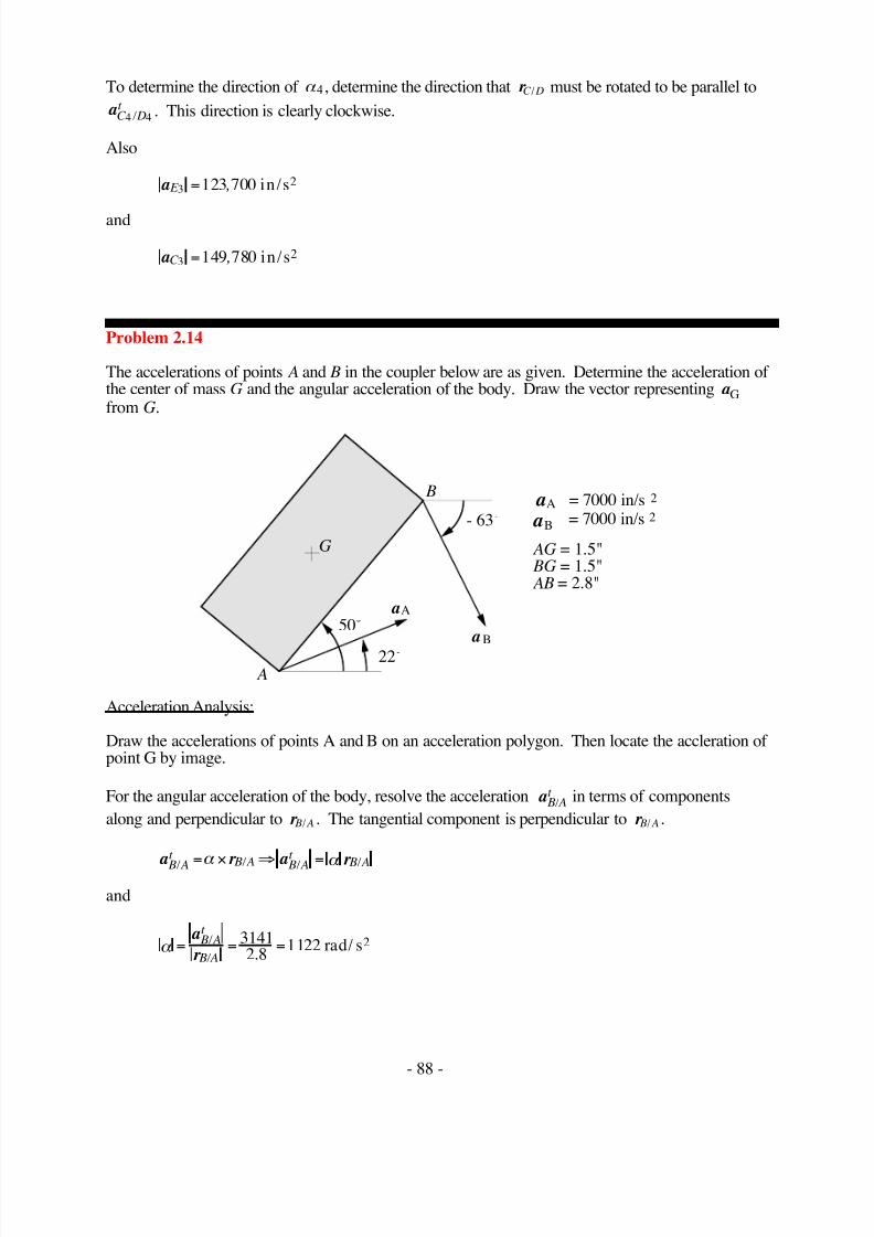
Problem 2.14
The accelerations of points A and B in the coupler below are as given. Determine the acceleration of the center of mass G and the angular acceleration of the body. Draw the vector representing aGfrom G.
G
B
A
a B
22˚
50˚
- 63˚
Aa
Aa = 7000 in/s 2
aB = 7000 in/s 2
AG = 1.5" BG = 1.5" AB = 2.8"
Acceleration Analysis:
Draw the accelerations of points A and B on an acceleration polygon. Then locate the accleration of point G by image.
For the angular acceleration of the body, resolve the acceleration a B At / in terms of components
along and perpendicular to r B A/ . The tangential component is perpendicular to r B A/ .
a r a r B A
t
B A B A
t
B A / / / / = × ⇒ =α α
and
α = = =
a
r
B At
B A
/
/ .31412 8
1122 rad/ s2

7/17/2019 Chapter 2. Graphical Position Velocity ...
http://slidepdf.com/reader/full/chapter-2-graphical-position-velocity- 42/118
- 89 -
o'
2000 in/s
Acceleration Scale
2
A
G
B a'
b'
g'
aB/ At
aG
To determine the direction of α , determine the direction that r B A/ must be rotated to be parallel to
a B At / . This direction is clearly clockwise.
Also
aG = 6980 in / s2
in the direction shown.

7/17/2019 Chapter 2. Graphical Position Velocity ...
http://slidepdf.com/reader/full/chapter-2-graphical-position-velocity- 43/118
- 90 -
Problem 2.15
Crank 2 of the push-link mechanism shown in the figure is driven at a constant angular velocity ωω ω ω 2
= 60 rad/s (CW). Find the velocity and acceleration of point F and the angular velocity andacceleration of links 3 and 4.
Y
X A
B
2
3 4
30˚
C
D
E F
AB = 15 cm BC = 29.5 cmCD = 30.1 cm AD = 7.5 cm BE = 14.75 cm EF = 7.5 cm
Position Analysis:
Draw the linkage to scale. First located the pivots A and D. Next locate B, then C, then E, then F.
Velocity Analysis:
v v v r v r A B B A B A B B A2 3 2 2 2 2 2 2 22 2 60 0 15 9= = = · = = = / / / ( . )ω ω m / s
v v vC B C B3 3 3 3= + / (1)
v v v r C C C D C D3 4 4 4 4= = = · / / ω
Now,
v r B B Am s3 9= ^ / ( ) / to
v r r C B C B C B3 3 3 / / / ( )= · ^ω to
v r r C C D C D4 4= · ^ωω / / ( )to
Solve Eq. (1) graphically with a velocity polygon. The velocity directions can be gotten directlyfrom the polygon. The magnitudes are given by:
v v
r C B
C B
C Bm s3 3
3 312 82 12 82
0 295 43 453 /
/
/ . /
..
.= = = =ω rad / s
Using velocity image,
vF m s3 4 94= . /

7/17/2019 Chapter 2. Graphical Position Velocity ...
http://slidepdf.com/reader/full/chapter-2-graphical-position-velocity- 44/118
- 91 -
in the direction shown.
o
2 m/s
Velocity Polygon
b2 b3, c3 c4,o'
100 m/s
Acceleration Polygon
2b2' b3',
f 3'
A
B
C
2
3 4
30°
5 cm
arB2 /A2
D
E F
a2
arC3 /B3
atC3 /B3
c 3' c 4',
atC4 /D4
arC4 /D4
From the directions given in the position and velocity polygons
ωω .. // 3 43 45 rad s CW =
Also,
v v
r C D
C D
C D4 4
4 411 39 11 39
0 301 37 844 /
/
/ .
..
.= = = =m / s rad / sωω
From the directions given in the position and velocity polygons
ωω 4 37 84= . rad / s CW
Acceleration Analysis:
a a a r B B
r B A B A2 3 2 2 2 2= = = · ·( ) / / ωω ωω

7/17/2019 Chapter 2. Graphical Position Velocity ...
http://slidepdf.com/reader/full/chapter-2-graphical-position-velocity- 45/118
- 92 -
a a a a aC C C D B C B3 4 4 4 3 3 3= = = + / /
a a a a a at
C D r
C D r
B A t
B A r
C B t
C B4 4 4 4 2 2 2 2 3 3 3 3 / / / / / / + = + + + (2)
Now,
a r r
C D C D m s4 4 42 2 237 84 0 301 430 99 / / . . . / = = =ωω in the direction opposite to rC D/ )
a r r
C B C B m s3 3 32 2 243 45 0 295 556 93 / / . . . / = = =ω in the direction opposite to rC B/ )
a r r
B A B A m s2 2 22 2 260 0 15 540 / / . / = = =ωω in the direction opposite to rB A/ )
a r a
r r t
C B C B
t C B
C BC B3 3
3 33 3 / /
/
/ / ( )= · = ^α α to
a r a
r r t
C D C D
t C D
C DC D4 4
4 44 4 / /
/
/ / ( )= · = ^α α to
Solve Eq. (2) graphically with an acceleration polygon. The acceleration directions can be gottendirectly from the polygon. The magnitudes are given by:
α 3 3 3 142 79
0 295 484= = =
a
r
t C B
C B
/
/
..
rad / s CW 2
Also,
α 4 4 4 41 01
0 301 136 = = =
a
r
t C D
C D
/
/
..
rad / s CCW 2
Using acceleration polygon,
aF m s3 256 2= /
in the direction shown.
Problem 2.16
For the straight-line mechanism shown in the figure, ωω ω ω 2 = 20 rad/s (CW) and αα α α 2 = 140 rad/s2
(CW). Determine the velocity and acceleration of point B and the angular acceleration of link 3.
A C
B
2
4
3
15o D
DA = 2.0" AC = 2.0" AB = 2.0"

7/17/2019 Chapter 2. Graphical Position Velocity ...
http://slidepdf.com/reader/full/chapter-2-graphical-position-velocity- 46/118
- 93 -
Velocity Analysis:
v v v r A A D A A D2 2 2 3 2 22= = = · / / ωω
v v v vC C A C A3 4 3 3 3= = + / (1)
Now,
v r r A A D A D3 2 2 2 22 20 2 40= = ⋅ = ⊥ω / / ( )in / s to
vC 3 in horizontal direction
v r v r r C A C AC A C A C A3 3 3 3 3 3 3 3 3 33 3 / / / / / ( )= × ⇒ = ⊥ω ω to
Solve Eq. (1) graphically with a velocity polygon. From the polygon,
v B3 77 3= . in/s
Also,
vC A3 3 40 / = in/s
or
ω 33 3
3 3
402
20= = =v
r
C A
C A
/
/
rad/sCCW
Also,
vC 3 20 7= . in/s
Acceleration Analysis:
a a a aC C A C A3 4 3 3 3= = + /
a a a a aC A Dr
A Dt
C Ar
C At
3 2 2 2 2 3 3 3 3= + + + / / / / (2)
Now,
aC 3 in horizontal direction
a r a r A Dr
A D A Dr
A D2 2 2 2 2 22 2 22 220 2 800 / / / / = × ×( ) ⇒ = ⋅ = ⋅ =ω ω ω in/s2
in the direction opposite to r A D/
a r a r r A Dt
A D A Dt
A D A D2 2 2 2 2 22 2 140 2 280 / / / / / ( )= × ⇒ = ⋅ = ⋅ = ⊥α α in / s to2
a r a r C Ar
C A C Ar
C A3 3 3 3 3 3 3 33 3 32 220 2 800 / / / / = × ×( ) ⇒ = ⋅ = ⋅ =ω ω ω in /s2
in the direction opposite to r C A3 3/

7/17/2019 Chapter 2. Graphical Position Velocity ...
http://slidepdf.com/reader/full/chapter-2-graphical-position-velocity- 47/118
- 94 -
a r a r r C At
C A C At
C A C A3 3 3 3 3 3 3 3 3 33 3 / / / / / ( )= × ⇒ = ⋅ ⊥α α to
Solve Eq. (2) graphically with a acceleration polygon. From the polygon,
a B3 955= in /s2
aC A3 3 280 / = in/s2
Also,
α 33 3
3 3
2802
140= = =
a
r
C At
C A
/
/ rad / s CCW2
AC
B
2
4
3
D
o
20 in/s
Velocity Polygon
a2 a3,
c3 , c4
b3
vC3
v A3 vC3 / A3
v B3
v B3 / A3
o'
400 in/s
Acceleration Polygon2
a2' a3',
aA2 / D 2
r
aA2/D 2
t
aC3c3'
aC3 / A3
r
aC3 / A3
t
b3'
aB3

7/17/2019 Chapter 2. Graphical Position Velocity ...
http://slidepdf.com/reader/full/chapter-2-graphical-position-velocity- 48/118
- 95 -
Problem 2.17
For the data given in the figure below, find the velocity and acceleration of points B and C . Assume
vA = 20 ft/s, aA = 400 ft/s2, ωω ω ω 2 = 24 rad/s (CW), and αα α α 2 = 160 rad/s2 (CCW).
Bω 2
15o
vA
aA
α 2
A
C
90˚
AB = 4.05" AC = 2.5" BC = 2.0"
Position AnalysisDraw the link to scale
o
a2
b2
c2
5 ft/sec
Velocity Polygon
o'
a2'
b2'
2'
80 ft/sec
Acceleration Polygon
2
aB2 /A2
r
a B2 /A2
t
c
Velocity Analysis:
v v v B A B A2 2 2 2= + / (1)
Now,

7/17/2019 Chapter 2. Graphical Position Velocity ...
http://slidepdf.com/reader/full/chapter-2-graphical-position-velocity- 49/118
- 96 -
v A ft 2 20= /sec in the positive vertical direction
v r v r B A B A B A B A in2 2 2 22 2 24 4 05 97 2 / / / / . . / sec= × ⇒ = ⋅ = ⋅ =ω ω
v r B A B A ft to2 2 8 1 / / . / sec( )= ⊥ in the positive vertical direction
Solve Eq. (1) graphically with a velocity polygon. From the polygon,
v B ft 2 11 9= . / sec
Also, from the velocity polygon,
vC ft 2 15 55= . / sec in the direction shown
Acceleration Analysis:
a a a a a a B A B A A B At
B Ar
2 2 2 2 2 2 2 2 2= + = + + / / / (2)
Now,
a A ft 2 400 2= /sec in the given direction
a B At
B Ar in ft 2 2 2
2 2160 4 05 648 54 / / . / sec / sec= ⋅ = ⋅ = =α
a B Ar
B Ar in ft 2 2 2
2 2 2 224 4 05 2332 194 / / . / sec / sec= ⋅ = ⋅ = =ω
Solve Eq. (2) graphically with an acceleration polygon. From the polygon,
a B ft 2 198 64 2= . / sec
in the direction shown. Determine the acceleration of point C by image. From the accelerationimage,
aC ft 2 289 4 2= . / sec
in the direction shown.
7/17/2019 Chapter 2. Graphical Position Velocity ...
http://slidepdf.com/reader/full/chapter-2-graphical-position-velocity- 50/118
- 97 -
Problem 2.18
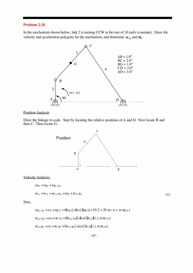
In the mechanism shown below, link 2 is turning CCW at the rate of 10 rad/s (constant). Draw the
velocity and acceleration polygons for the mechanism, and determine aG3 and αα α α 4.
2
3
4
A
C
B
D
G
αω2 2,
90˚
AB = 1.0" BC = 2.0" BG = 1.0"CD = 3.0" AD = 3.0"
Position Analysis
Draw the linkage to scale. Start by locating the relative positions of A and D. Next locate B andthen C. Then locate G.
Velocity Analysis:
v v v B B B A3 2 2 2= = /
v v v v vC C C D B C B3 4 4 4 3 3 3= = = + / / (1)
Now,
v r v r r B A B A B A B A B A2 2 2 2 10 2 20 / / / / / ( )= × ⇒ = ⋅ = ⋅ = ⊥ω ω in / s to
v r v r r C D C D C D C D C D4 4 4 44 4 / / / / / ( )= × ⇒ = ⋅ ⊥ω ω to
v r v r r C B C B C B C B C B3 3 3 33 3 / / / / / ( )= × ⇒ = ⋅ ⊥ω ω to

7/17/2019 Chapter 2. Graphical Position Velocity ...
http://slidepdf.com/reader/full/chapter-2-graphical-position-velocity- 51/118
- 98 -
Solve Eq. (1) graphically with a velocity polygon.
From the polygon,
vC B3 3 14 4 / .= in/s
vC D4 4 13 7 / .= in/s
in the direction shown.
Now
ω 33 3 11 4
25 7= = =
v
r
C B
C B
/
/
. . rad/s
and
ω 44 4 13 7
34 57= = =
v
r
C D
C D
/
/
. . rad/s
To determine the direction of ω 3, determine the direction that r C B/ must be rotated to be parallel to
vC B3 3 / . This direction is clearly clockwise.
To determine the direction of ω 4 , determine the direction that r C D/ must be rotated to be parallel to
vC D4 4 / . This direction is clearly counterclockwise.
The velocity of point G3
v v v r r G B G B G B G B3 3 3 3 3 3 5 7 1 5 7= + = × = ⋅ = ⋅ = / / / . .ω ω in/s
Acceleration Analysis:
a a a B B B A3 2 2 2= = /
a a a a aC C C D B C B3 4 4 4 3 3 3= = = + / /
a a a a a aC Dr
C Dt
B Ar
B At
C Br
C Bt
4 4 4 4 2 2 2 2 3 3 3 3 / / / / / / + = + + +(2)
Now,

7/17/2019 Chapter 2. Graphical Position Velocity ...
http://slidepdf.com/reader/full/chapter-2-graphical-position-velocity- 52/118
- 99 -
a r a r B Ar
B A B Ar
B A2 2 2 22 2 22 210 1 100 / / / / = × ×( ) ⇒ = ⋅ = ⋅ =ω ω ω in /s2
in the direction of - r B A2 2/
a r a r B At
B A B At
B A2 2 2 22 2 0 / / / / = × ⇒ = =α α
a r a r C Br C B C Br C B3 3 3 33 3 3 2 25 7 2 64 98 / / / / . .= × ×( ) ⇒ = ⋅ = ⋅ =ω ω ω in/s2
in the direction of - r C B/
a r a r r C Bt
C B C Bt
C B C B3 3 3 33 3 / / / / / ( )= × ⇒ = ⋅ ⊥α α to
a r a r C Dr
C D C Dr
C D in4 4 4 44 4 4
2 2 24 57 3 62 66 / / / / . . /sec= × ×( ) ⇒ = ⋅ = ⋅ =ω ω ω
in the direction of - rC D/
a r a r r C D
t
C D C D
t
C D C Dto
4 4 4 44 4 / / / / / ( )= × ⇒ = ⋅ ⊥α α
Solve Eq. (2) graphically for the accelerations.

7/17/2019 Chapter 2. Graphical Position Velocity ...
http://slidepdf.com/reader/full/chapter-2-graphical-position-velocity- 53/118
- 100 -
From the acceleration polygon,
aC Bt
3 338 / = in/s2
aC Dt
4 4128 / = in/s2
Then,
α 33 3 38
219= = =
a
r
C Bt
C B
/
/ rad/s2
α 44 4 128
342 67= = =
a
r
C Dt
C D
/
/ . rad/s2
To determine the direction of α 3 , determine the direction that r C B/ must be rotated to be parallel to
aC Bt
3 3 / . This direction is clearly counterclockwise.
To determine the direction ofα
4, determine the direction thatr C D/ must be rotated to be parallel to
aC Dt
4 4 / . This direction is clearly clockwise.
Determine the acceleration of point G3
a a a a a aG B G B B G Br
G Bt
3 3 3 3 2 3 3 3 3= + = + + / / /
a r a r G Bt
G B G Bt
G B in3 3 3 33 3
219 1 19 / / / / /sec= × ⇒ = ⋅ = ⋅ =α α
a r a r G Br
G B G Br
G B in3 3 3 33 3 3
2 2 25 7 1 32 49 / / / / . . / sec= × ×( ) ⇒ = ⋅ = ⋅ =ω ω ω
From the acceleration polygon,
aG3 116= in /s2
Problem 2.19
If ωω ω ω 2 = 100 rad/s CCW (constant) find the velocity and acceleration of point E .
A
C
AB = 1.0" BC = 1.75"CD = 2.0" DE = 0.8" AD = 3.0"
ω 2
B
D
E
70˚2
3
4

7/17/2019 Chapter 2. Graphical Position Velocity ...
http://slidepdf.com/reader/full/chapter-2-graphical-position-velocity- 54/118
- 101 -
Position Analysis
Draw the linkage to scale. Start by locating the relative positions of A and D. Next locate B andthen C. Then locate E.
Velocity Analysis:
v v v B B B A3 2 2 2= = /
v v v v vC C C D B C B3 4 4 4 3 3 3= = = + / / (1)
Now,
v r v r r B A B A B A B A B A2 2 2 2 100 1 100 / / / / / ( )= × ⇒ = ⋅ = ⋅ = ⊥ω ω in / s to
v r v r r C D C D C D C D C D4 4 4 44 4 / / / / / ( )= × ⇒ = ⋅ ⊥ω ω to
v r v r r C B C B C B C B C B3 3 3 33 3 / / / / / ( )= × ⇒ = ⋅ ⊥ω ω to
Solve Eq. (1) graphically with a velocity polygon.
From the polygon,
vC B3 3 77 5 / .= in /s
vC D4 4 71 / = in/s
in the direction shown.

7/17/2019 Chapter 2. Graphical Position Velocity ...
http://slidepdf.com/reader/full/chapter-2-graphical-position-velocity- 55/118
- 102 -
Now
ω 33 3 77 5
1 7544 29= = =
v
r
C B
C B
/
/
..
. rad/s
and
ω 4 4 4 712 35 5= = =v
r C DC D
/ /
. rad/s
To determine the direction of ω 3, determine the direction that r C B/ must be rotated to be parallel to
vC B3 3 / . This direction is clearly clockwise.
To determine the direction of ω 4 , determine the direction that r C D/ must be rotated to be parallel to
vC D4 4 / . This direction is clearly counterclockwise.
The velocity of point E3
v v v r r E D E D D E D E 4 4 4 4
4 4 35 5 0 8 28 4= + = × = ⋅ = ⋅ = / / / . . .ω ω in /s
Acceleration Analysis:
a a a B B B A3 2 2 2= = /
a a a a aC C C D B C B3 4 4 4 3 3 3= = = + / /
a a a a a aC Dr
C Dt
B Ar
B At
C Br
C Bt
4 4 4 4 2 2 2 2 3 3 3 3 / / / / / / + = + + +(2)
Now,
a r a r B Ar B A B Ar B A2 2 2 22 2 2 2 2100 1 10 000 / / / / ,= × ×( ) ⇒ = ⋅ = ⋅ =ω ω ω in/s2
in the direction of - r B A2 2/
a r a r B At
B A B At
B A2 2 2 22 2 0 / / / / = × ⇒ = =α α
a r a r C Br
C B C Br
C B3 3 3 33 3 32 244 29 1 75 3432 8 / / / / . . .= × ×( ) ⇒ = ⋅ = ⋅ =ω ω ω in/s2
in the direction of - r C B/
a r a r r C Bt
C B C Bt
C B C B3 3 3 33 3 / / / / / ( )= × ⇒ = ⋅ ⊥α α
to
a r a r C Dr
C D C Dr
C D in4 4 4 44 4 4
2 2 235 5 2 2520 5 / / / / . . / sec= × ×( ) ⇒ = ⋅ = ⋅ =ω ω ω
in the direction of - rC D/
a r a r r C Dt
C D C Dt
C D C Dto4 4 4 44 4 / / / / / ( )= × ⇒ = ⋅ ⊥α α
Solve Eq. (2) graphically with acceleration.

7/17/2019 Chapter 2. Graphical Position Velocity ...
http://slidepdf.com/reader/full/chapter-2-graphical-position-velocity- 56/118
- 103 -
From the acceleration polygon,
aC Bt
3 33500 / = in/s2
aC Dt
4 410 900 / ,= in/s2
Then,
α 33 3 3500
1 752000= = =
a
r
C Bt
C B
/
/ .rad/s2
α 44 4 10 900
25450= = =
a
r
C Dt
C D
/
/
,rad/s2
To determine the direction of α 3 , determine the direction that r C B/ must be rotated to be parallel toaC B
t 3 3 / . This direction is clearly counterclockwise.
To determine the direction of α 4, determine the direction that r C D/ must be rotated to be parallel to
aC Dt
4 4 / . This direction is clearly clockwise.
Determine the acceleration of point E4
a a a a a E D E D E Dr
E Dt
4 4 4 4 4 4 4 4= + = + / / /

7/17/2019 Chapter 2. Graphical Position Velocity ...
http://slidepdf.com/reader/full/chapter-2-graphical-position-velocity- 57/118
- 104 -
a r a r E Dt
E D E Dt
E D in4 4 4 44 4
25450 0 8 4360 / / / / . / sec= × ⇒ = ⋅ = ⋅ =α α
a r a r E Dr
E D E Dr
E D in4 4 4 44 4 4
2 2 235 5 0 8 1008 2 / / / / . . . / sec= × ×( ) ⇒ = ⋅ = ⋅ =ω ω ω
From the acceleration polygon,
a E 4
4600= in/s2
Problem 2.20
Draw the velocity polygon to determine the velocity of link 6. Points A, C , and E have the samevertical coordinate.
2
4
5
A
B
C
D
E
3
6
= 6ω2rads
1
AB = 1.80" BC = 1.95"CD = 0.75" DE = 2.10"
50˚
Velocity Analysis:
v v v B B B A3 2 2 2
= = /
v v v vC C B C B4 3 3 3 3= = + / (1)
v v D D5 3=
v v v v E E D E D5 6 5 5 5= = + / (2)
Now,
v r v r r B A B A B A B A B A2 2 2 2 2 2 2 2 2 22 2 6 1 8 10 8 / / / / / . . ( )= × ⇒ = ⋅ = ⋅ = ⊥ω ω in / s to
vC 3 is in the vertical direction. Then,
v r v r r C B C B C B C B C B3 3 3 3 3 3 3 3 3 33 3 / / / / / ( )= × ⇒ = ⋅ ⊥ω ω to
Solve Eq. (1) graphically with a velocity polygon. From the polygon, using velocity image,
v in s D3 18 7= . /

7/17/2019 Chapter 2. Graphical Position Velocity ...
http://slidepdf.com/reader/full/chapter-2-graphical-position-velocity- 58/118
- 105 -
2
4
5
A
B
C
D
E
3
6
b3
c3
d3
o
10 in/sec
Velocity Polygon
e5
d5
Now,
v E 5 in horizontal direction
v r v r r E D E D E D E D E D5 5 5 55 5 / / / / / ( )= × ⇒ = ⋅ ⊥ω ω to
Solve Eq. (2) graphically with a velocity polygon. From the polygon, using velocity image,
v v in s E E 5 6 8 0= = . /

7/17/2019 Chapter 2. Graphical Position Velocity ...
http://slidepdf.com/reader/full/chapter-2-graphical-position-velocity- 59/118
- 106 -
Problem 2.21
Link 2 of the linkage shown in the figure has an angular velocity of 10 rad/s CCW. Find theangular velocity of link 6 and the velocities of points B, C , and D.
A
D
C
B
2
4
6
5
ω 2
EF
3
X
Y
0.3"
AE = 0.7"AB = 2.5"AC = 1.0"BC = 2.0"EF = 2.0"CD = 1.0"DF = 1.5"
θ 2
= 135˚θ 2
Position Analysis
Locate points E and F and the slider line for B. Draw link 2 and locate A. Then locate B. Nextlocate C and then D.
Velocity Analysis:
v v v A A A E 3 2 2 2= = /
v v v v B B A B A4 3 3 3 3= = + / (1)
Find vC 3 by image.
v vC C 5 3=
v v v v v D D D F C D C 5 6 6 6 5 5 5= = = + / / (2)
Now,
v B3 in horizontal direction
v r v r r A E A E A E A E A E 2 2 2 22 2 10 0 7 7 / / / / / . ( )= × ⇒ = ⋅ = ⋅ = ⊥ω ω in / s to
v r v r r B A B A B A B A B A3 3 3 33 3 / / / / / ( )= × ⇒ = ⋅ ⊥ω ω to
Solve Eq. (1) graphically with a velocity polygon. From the polygon,

7/17/2019 Chapter 2. Graphical Position Velocity ...
http://slidepdf.com/reader/full/chapter-2-graphical-position-velocity- 60/118
- 107 -
E
A
B
C
D
F
2
3
4
6
Slider Line
Velocity Polygon
2.5 in/s
a3
o
f 6b3
c3c5
d5
v B3 3 29=
. in/s
Using velocity image,
v vC C 5 3 6 78= = . in/ s
Now,
v r v r r D F D F D F D F D F to6 6 6 66 6 / / / / / ( )= × ⇒ = ⋅ ⊥ω ω
v r v r r D C D C D C D C D C to5 5 5 55 5 / / / / / ( )= × ⇒ = ⋅ ⊥ω ω
Solve Eq. (2) graphically with a velocity polygon. From the polygon,
v v v D D D F 5 6 6 6 6 78= = = / . in/s
or
ω 66 6
6 6
6 781 5
4 52= = =v
r D F
D F
/
/
..
. rad/sCCW

7/17/2019 Chapter 2. Graphical Position Velocity ...
http://slidepdf.com/reader/full/chapter-2-graphical-position-velocity- 61/118
- 108 -
Problem 2.22
The linkage shown is used to raise the fabric roof on convertible automobiles. The dimensions atgiven as shown. Link 2 is driven by a DC motor through a gear reduction. If the angular velocity,
ωω ω ω
2 = 2 rad/s, CCW, determine the linear velocity of point J , which is the point where the linkageconnects to the automobile near the windshield.
AB = 3.5" AC = 15.37" BD = 16"CD = 3"CE = 3.62" EG = 13.94"GF = 3.62" HF = 3"
FC = 13.62" HI = 3.12"GI = 3.62" HL = 0.75"KC = 0.19" JH = 17"
B A
E
C
D
F
G
H
I
J H
F C D
K L
2
3
4
6
7
85
3
12ω
Detail of Link 3
110˚
Position Analysis:
Draw linkage to scale. Start with link 2 and locate points C and E. Then locate point D. Thenlocate points F and H. Next locate point G. Then locate point I and finally locate J.
Velocity Analysis:
The equations required for the analysis are:
v v r v r C C A C A C C A2 2 2 2 2 2 2 22 2 2 15 37 30 74= = × ⇒ = = ⋅ = / / / ( . ) .ω ω in/s
v vC C 3 2=
v v v v v D D D B C D C 3 4 4 4 3 3 3= = = + / / (1)
v v v v v v vG G G F G F E G E 5 6 7 5 5 5 6 6 6= = = + = + / /
v vF F 5 3=
v v E E 6 2=
So,

7/17/2019 Chapter 2. Graphical Position Velocity ...
http://slidepdf.com/reader/full/chapter-2-graphical-position-velocity- 62/118
- 109 -
v v v vF G F E G E 5 5 5 6 6 6+ = + / / (2)
v v v v v v I I G I G H I H 7 8 7 7 7 8 8 8= = + = + / /
v v H H 8 3=
So,
v v v vG I G H I H 7 7 7 8 8 8+ = + / / (3)
c3
d3
f 3
h3
e2
g6
i8
j8
AB
CD
E
G
FH
I
J
2 4
3
6
5
7
8
10 in/s
Velocity Polygon
o

7/17/2019 Chapter 2. Graphical Position Velocity ...
http://slidepdf.com/reader/full/chapter-2-graphical-position-velocity- 63/118
- 110 -
Now,
v r C C A3 30 74= ⊥. ( ) / in / s to
v r r D C D C D C 3 3 3 / / / ( )= × ⊥ω to
v r r D B D B D B4 4 4 / / / ( )= × ⊥ω to
Solve Eq. (1) graphically with a velocity polygon. The velocity directions can be gotten directlyfrom the polygon. The magnitudes are given by:
v D4 30 9= . in /s
Using velocity image of link 3, find the velocity of points F and H and of link 2, find the velocity of point E.
vF 5 30 5= . in /s
v H 3 30 3= . in /s
and
v E 6 3 80= . in/s
Now,
v r r G F G F G F 5 5 5 / / / ( )= × ⊥ω to
v r r G E G E G E 6 6 6 / / / ( )= × ⊥ω to
Solve Eq. (2) graphically with a velocity polygon. The velocity directions can be gotten directlyfrom the polygon. The magnitudes are given by:
vG6 37 8= . in/s
Now,
v r r I G I G I G7 7 7 / / / ( )= × ⊥ω to
v r r I H I H I H 8 8 8 / / / ( )= × ⊥ω to
Solve Eq. (3) graphically with a velocity polygon. Using velocity polygon of link 8
v J 8 73 6= . in/s

7/17/2019 Chapter 2. Graphical Position Velocity ...
http://slidepdf.com/reader/full/chapter-2-graphical-position-velocity- 64/118
- 111 -
Problem 2.23
In the mechanism shown, determine the sliding velocity of link 6 and the angular velocities of links3 and 5.
2
4
5
6
B
C
D
E
F
= 3ω2rads
50˚
10.4"
2.0"
29.5"
A
AB = 12.5" BC = 22.4" DC = 27.9"CE = 28.0"
DF = 21.5"
3
34˚
Position Analysis
First locate Points A and E. Next draw link 2 and locate B. Then locate point C by drawing a circlecentered at B and 22.4 inches in radius, and finding the intersection with a circle centered at E and
of 28 inches in radius. Find D by drawing a line 27.9 inches long at an angle of 34˚ relative to lineBC. Locate the slider line 2 inches above point E. Draw a circle centered at D and 21.5 inches in
radius and find the intersections of the circle with the slider line. Choose the proper intersectioncorresponding to the position in the sketch.
Velocity Analysis
Compute the velocity of the points in the same order that they were drawn. The equations for thefour bar linkage are:
v v r B B A B A2 2 2 2= = × / / ω
v v B B3 2=
v v vC B C B3 3 3 3= + /

7/17/2019 Chapter 2. Graphical Position Velocity ...
http://slidepdf.com/reader/full/chapter-2-graphical-position-velocity- 65/118
- 112 -
A
B
C
D
10 in/sec
Velocity Polygon
o
E
c 3
F
b 3
d 3
f 3
Also,
v v v v vC C E C E C E 3 4 4 4 4 4 4= = + = / /
where,
v r B B A in2 2 3 12 5 37 5= = ⋅ =ω / . . / sec
v r C B C B to CB3 3 3 / / ( )= × ⊥ω
v r C E C E to CE 4 4 4 / / ( )= × ⊥ω
The velocity of C3 (and C4) can then be found using the velocity polygon. After the velocity of C3is found, find the velocity of D3 by image. Then,
7/17/2019 Chapter 2. Graphical Position Velocity ...
http://slidepdf.com/reader/full/chapter-2-graphical-position-velocity- 66/118
- 113 -
v v D D5 3=
v v vF D F D5 5 5 5= + /
and
v vF F 5 6=
where
v r v r F D F D C F D to FD5 5 55 5 / / / ( )= × ⇒ = ⊥ω ω
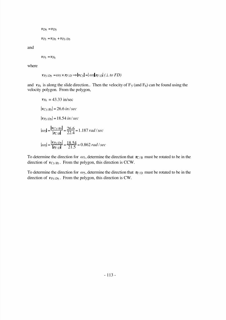
and vF 6 is along the slide direction.. Then the velocity of F5 (and F6) can be found using thevelocity polygon. From the polygon,
vF 6 = 43.33 in/sec
vC B in3 3 26 6 / . / sec=
vF D in5 5 18 54 / . / sec=
ω 33 3 26 6
22 41 187= = =
v
r C B
C Brad
/
/
.
. . / sec
ω 55 5 18 54
21 50 862= = =
v
r F D
F Drad
/
/
..
. / sec
To determine the direction for ω 3, determine the direction that rC B/ must be rotated to be in the
direction of vC B3 3 / . From the polygon, this direction is CCW.
To determine the direction for ω 5, determine the direction that rF D/ must be rotated to be in the
direction of vF D5 5 / . From the polygon, this direction is CW.

7/17/2019 Chapter 2. Graphical Position Velocity ...
http://slidepdf.com/reader/full/chapter-2-graphical-position-velocity- 67/118
- 114 -
Problem 2.24
In the mechanism shown, vA2 = 15 m/s. Draw the velocity polygon, and determine the velocity of point D on link 6 and the angular velocity of link 5.
1vA2
= 15 m/s
2
3
4
5
A
C
B
D
45˚
2.05"
AC = 2.4" BD = 3.7" BC = 1.2"
X
Y
2.4"
6
Velocity Analysis:
v v A A3 2=
v v v vC C A C A4 3 3 3 3= = + / (1)
v v B B3 5=
v v v v D D B D B5 6 5 5 5= = + / (2)
Now,
v A m3 15= /sec in vertical direction
vC 3 in horizontal direction
v r v r r C A C A C A C A C Ato3 3 3 3 3 3 3 3 3 33 3 / / / / / ( )= × ⇒ = ⋅ ⊥ω ω
Solve Eq. (1) graphically with a velocity polygon. From the polygon, using velocity image,
v v B B m3 5 14 44= = . / sec
Now,

7/17/2019 Chapter 2. Graphical Position Velocity ...
http://slidepdf.com/reader/full/chapter-2-graphical-position-velocity- 68/118
- 115 -
3
4
5
C
B
D
2A
6
a3
c3o
10 m/sec
Velocity Polygon
b3b5b
d5
v D5 along the inclined path
v r v r r D B D B D B D B D Bto5 5 5 5 5 5 5 5 5 55 5 / / / / / ( )= × ⇒ = ⋅ ⊥ω ω
Solve Eq. (2) graphically with a velocity polygon. From the polygon,
v D m6 12 31= . / sec
Also,
v D B m5 5 16 61 / . / sec=
or
ω 55 5 16 605
3 74 488= = =
vr D B
D Brad CCW
/
/
..
. / sec

7/17/2019 Chapter 2. Graphical Position Velocity ...
http://slidepdf.com/reader/full/chapter-2-graphical-position-velocity- 69/118
- 116 -
Problem 2.25
In the mechanism shown below, points E and B have the same vertical coordinate. Find thevelocities of points B, C , and D of the double-slider mechanism shown in the figure if Crank 2rotates at 42 rad/s CCW.
A
D
C
2
6
5
B
4
33
E
ω 2
0.75"
60˚
EA = 0.55" AB = 2.5"
AC = 1.0"CB = 1.75"CD = 2.05"
Position Analysis
Locate point E and draw the slider line for B. Also draw the slider line for D relative to E. Drawlink 2 and locate A. Then locate B. Next locate C and then D.
Velocity Analysis:
v v v A A A E 3 2 2 2= = /
v v v v B B A B A4 3 3 3 3= = + / (1)
v vC C 5 3=
v v v v D D C D C 5 6 5 5 5= = + / (2)
Now,
v B3 in horizontal direction

7/17/2019 Chapter 2. Graphical Position Velocity ...
http://slidepdf.com/reader/full/chapter-2-graphical-position-velocity- 70/118
- 117 -
A
D
C
2
6
5
B
4
3
3
E
10 in/sec
Velocity Polygon
b3
a3
c3 d5
o
v r v r r A E A E A E A E A E in to2 2 2 2 2 22 2 42 0 55 23 1 / / / / / . . / sec ( )= × ⇒ = ⋅ = ⋅ = ⊥ω ω
v r v r r B A B A B A B A B Ato3 3 3 3 3 33 3 / / / / / ( )= × ⇒ = ⋅ ⊥ω ω
Solve Eq. (1) graphically with a velocity polygon. From the polygon,
v B in4 17 76= . / sec
Using velocity image,
vC in3 18 615= . / sec
Now,
v D5 in vertical direction
v r v r r D C D C D C D C D C to5 5 5 5 5 55 5 / / / / / ( )= × ⇒ = ⋅ ⊥ω ω
7/17/2019 Chapter 2. Graphical Position Velocity ...
http://slidepdf.com/reader/full/chapter-2-graphical-position-velocity- 71/118
- 118 -
Solve Eq. (2) graphically with a velocity polygon. From the polygon,
v D in5 5 63= . / sec
Problem 2.26
Given vA4 = 1.0 ft/s to the left, find vB6
.
A
B
C
D
2
4
5 E
6
3 X
Y
157.5˚
DE = 1.9"CD = 1.45" BC = 1.1" AD = 3.5" AC = 2.3"
1.0"
0.5"
Position Analysis
Draw the linkage to scale. Start by locating the relative positions of A, B and E. Next locate C and
D.
Velocity Analysis:
v v A A4 3=
v v v vC C A C A5 3 3 3 3= = + / (1)
v v D D3 2=
v v v D E D E 2 2 2 2= + / (2)

7/17/2019 Chapter 2. Graphical Position Velocity ...
http://slidepdf.com/reader/full/chapter-2-graphical-position-velocity- 72/118
- 119 -
v v v B C B C 5 5 5 5= + /
Now,
v A ft 4 1 0= . / sec in horizontal direction
v r v r r C A C A C A C A C Ato3 3 3 33 3 / / / / / ( )= × ⇒ = ⋅ ⊥ω ω
v r v r r D E D E D E D E D E to2 2 2 22 2 / / / / / ( )= × ⇒ = ⋅ ⊥ω ω
Solve Eq. (1) graphically with a velocity polygon.
From the polygon, using velocity image,
vC A ft 3 3 1 28 / . / sec=
and,
ω 33 3 1 28
2 30 56= = =
v
r C A
C A
/
/
..
. rad/s
To determine the direction of ω 3, determine the direction that r C A / must be rotated to be parallel tovC A3 3 / . This direction is clearly clockwise.
Now,
v B6 is horizontal direction
v r v r r B C B C B C B C B C to5 5 5 55 5 / / / / / ( )= × ⇒ = ⋅ ⊥ω ω

7/17/2019 Chapter 2. Graphical Position Velocity ...
http://slidepdf.com/reader/full/chapter-2-graphical-position-velocity- 73/118
- 120 -
Solve Eq. (2) graphically with a velocity polygon. From the polygon,
v B ft 6 1 23= . / sec
Problem 2.27
If vA2 = 10 cm/s as shown, find vC5
.
Position Analysis
Draw the linkage to scale. Start by locating the relative positions of D, F and G. Next locate A andB. Then locate E and C.
Velocity Analysis:
v v A A3 2=
v v v B A B A3 3 3 3= + / (1)
v v B B4 3=
v v v v B F B F B F 4 4 4 4 4 40= + = + / / (2)
v v E E 5 4=
v v vG E G E 5 5 5 5= + /

7/17/2019 Chapter 2. Graphical Position Velocity ...
http://slidepdf.com/reader/full/chapter-2-graphical-position-velocity- 74/118
- 121 -
v vG G6 5=
Now,
v A cm2 10= /sec ( ) / ⊥ to A C r
v r v r r B A B A B A B A B Ato3 3 3 33 3 / / / / / ( )= × ⇒ = ⋅ ⊥ω ω
v r v r r B F B F B F B F B F to4 4 4 44 4 / / / / / ( )= × ⇒ = ⋅ ⊥ω ω
From the polygon,
v B cm4 6 6= . / sec
Using velocity image,
v E cm4 3 12= . / sec
Now,
vG6 is horizontal direction
v r v r r G E G E G E G E G E to5 5 5 55 5 / / / / / ( )= × ⇒ = ⋅ ⊥ω ω
For the velocity image
draw a line ⊥ to C E r / at e
draw a line ⊥ to C E r / at g
and find the point “c”
From the velocity polygon
v B cm6 3 65= . / sec

7/17/2019 Chapter 2. Graphical Position Velocity ...
http://slidepdf.com/reader/full/chapter-2-graphical-position-velocity- 75/118
- 122 -
Problem 2.28
If vA2 = 10 in/s as shown, find the angular velocity of link 6.
23
4
56
A
v 2A
27˚
AB = 1.0" AD = 2.0" AC = 0.95"CE = 2.0" EF = 1.25" BF = 3.85"
B
C D
E
F
Position Analysis
Draw the linkage to scale. Start by locating the relative positions of B, D and F. Next locate A andC. Then locate E.
Velocity Analysis:
v v A A3 2=
v v v D A D A3 3 3 3= + / (1)
v v D D4 3=
v vC C 5 3=
v v v E C E C 5 5 5 5= + / (2)
v v E E 6 5=
v v v v E F E F E F 6 6 6 6 6 60= + = + / /
Now,
v A in2 10= /sec

7/17/2019 Chapter 2. Graphical Position Velocity ...
http://slidepdf.com/reader/full/chapter-2-graphical-position-velocity- 76/118
- 123 -
v r v r r D A D A D A D A D Ato3 3 3 33 3 / / / / / ( )= × ⇒ = ⋅ ⊥ω ω
From the polygon,
v D A in3 3 9 1 / . / sec=
Using velocity image,
r r v v D A C A D A C A / / / / : := 3 3 3 3
vC A in3 3 4 32 / . / sec=
Now,
v r v r r E C E C E C E C E C to5 5 5 55 5 / / / / / ( )= × ⇒ = ⋅ ⊥ω ω
v r v r r E F E F E F E F E F to6 6 6 66 6 / / / / / ( )= × ⇒ = ⋅ ⊥ω ω
from the velocity polygon
v E in6 2 75= . / sec
and
ω 6 6 6 2 752 1 375= = =vr E F E F
/ /
. . rad/s
To determine the direction of ω 6 , determine the direction that r E F / must be rotated to be parallel to
v E F 6 6 / . This direction is clearly counterclockwise.

7/17/2019 Chapter 2. Graphical Position Velocity ...
http://slidepdf.com/reader/full/chapter-2-graphical-position-velocity- 77/118
- 124 -
Problem 2.29
The angular velocity of link 2 of the mechanism shown is 20 rad/s, and the angular acceleration is100 rad/s2 at the instant being considered. Determine the linear velocity and acceleration of pointF
6.
D 2
3
4
5
6
C
B
E
F
ω2
α2 ,
A
115˚
2"
0.1"
2.44"
EF = 2.5"CD = 0.95" AB = 0.5" BC = 2.0"CE = 2.4" BE = 1.8"
Position Analysis
Draw the linkage to scale. Start by locating the relative positions of A and D. Next locate B andthen C. Then locate E and finally F.
Velocity Analysis:
The required equations for the velocity analysis are:
v v v B B B A3 2 2 2= = /
v v v v vC C C D B C B3 4 4 4 3 3 3= = = + / / (1)
v v E E 5 3=
v v v vF F E F E 5 6 5 5 5= = + / (2)
Now,
v r v r r B A B A B A B A B A2 2 2 2 2 2 2 2 2 22 2 20 0 5 10 / / / / / . ( )= × ⇒ = ⋅ = ⋅ = ⊥ω ω in / s to
v r v r r C D C D C D C D C D4 4 4 4 4 4 4 4 4 44 4 / / / / / ( )= × ⇒ = ⋅ ⊥ω ω to
v r v r r C B C B C B C B C B3 3 3 3 3 3 3 3 3 33 3 / / / / / ( )= × ⇒ = ⋅ ⊥ω ω to
Solve Eq. (1) graphically with a velocity polygon. From the polygon and using velocity image,

7/17/2019 Chapter 2. Graphical Position Velocity ...
http://slidepdf.com/reader/full/chapter-2-graphical-position-velocity- 78/118
- 125 -
vC B3 3 6 59 / .= in/s
or
ω 33 3
3 3
6 592
3 29= = =v
r C B
C B
/
/
. . rad/sCCW
Also,
vC D4 4 8 19 / .= in/s
or
ω 44 4
4 4
8 190 95
8 62= = =v
r C D
C D
/
/
.
. . rad/sCW
And,
v E 5 5 09= . in/s
Now,
vF 5 in horizontal direction
v r v r r F E F E F E F E F E 5 5 5 5 5 5 5 5 5 55 5 / / / / / ( )= × ⇒ = ⋅ ⊥ω ω to
Solve Eq. (2) graphically with a velocity polygon. From the polygon,
vF E 5 5 3 97 / .= in /s
or
ω 55 5
5 5
3 972 5
1 59= = =v
r F E
F E
/
/
..
. rad/s CCW
Also,
vF 6 3 79= . in/s
Acceleration Analysis:
a a a B B B A3 2 2 2= = /
a a a a aC C C D B C B3 4 4 4 3 3 3= = = + / /
a a a a a aC Dr
C Dt
B Ar
B At
C Br
C Bt
4 4 4 4 2 2 2 2 3 3 3 3 / / / / / / + = + + +(3)

7/17/2019 Chapter 2. Graphical Position Velocity ...
http://slidepdf.com/reader/full/chapter-2-graphical-position-velocity- 79/118
- 126 -
b3e5
o
5 in/sec
Velocity Polygon
f 5
b'3
c'3
e'5
o'
50 in/s
Acceleration Polygon2
f'5
1 aF5 /E5
t
1 aF5
1a E5
D
2
3
4
5
C
B
EF
A
1a F5 /E5
r
1aC3 /B3
t
1aC3 /B3r
1 aC4/D4t
1aC4 /D4r
1aB2 /A2r
1aB2 /A2t
c3
a a E E 5 3=
a a a aF F E F E 5 6 5 5 5= = + /
a a a aF E F E r
F E t
5 5 5 5 5 5= + + / / (4)
Now,
a r a r B Ar
B A B Ar
B A2 2 2 2 2 2 2 22 2 22 220 0 5 200 / / / / .= × ×( ) ⇒ = ⋅ = ⋅ =ω ω ω in /s2

7/17/2019 Chapter 2. Graphical Position Velocity ...
http://slidepdf.com/reader/full/chapter-2-graphical-position-velocity- 80/118
- 127 -
in the direction of - r B A2 2/
a r a r r B At
B A B At
B A B A2 2 2 2 2 2 2 2 2 22 2 100 0 5 50 / / / / / . ( )= × ⇒ = ⋅ = ⋅ = ⊥α α in / s to2
a r a r C Br
C B C Br
C B3 3 3 3 3 3 3 33 3 32 23 29 2 21 6 / / / / . .= × ×( ) ⇒ = ⋅ = ⋅ =ω ω ω in/s2
in the direction of - r C B3 3/
a r a r r C Bt
C B C Bt
C B C B3 3 3 3 3 3 3 3 3 33 3 / / / / / ( )= × ⇒ = ⋅ ⊥α α to
a r a r C Dr
C D C Dr
C D4 4 4 4 4 4 4 44 4 42 28 62 0 95 70 6 / / / / . . .= × ×( ) ⇒ = ⋅ = ⋅ =ω ω ω in/s2
in the direction of - r C D4 4/
a r a r r C Dt
C D C Dt
C D C D4 4 4 4 4 4 4 4 4 44 4 / / / / / ( )= × ⇒ = ⋅ ⊥α α to
Solve Eq. (3) graphically with an acceleration polygon. From the polygon, using accelerationimage,
a E 5 252 0= . in /s2
Now,
aF 5 in horizontal direction
a r a r F E r
F E F E r
F E 5 5 5 5 5 5 5 55 5 52 21 59 2 5 6 32 / / / / . . .= × ×( ) ⇒ = ⋅ = ⋅ =ω ω ω in/s2
in the direction of - r F E 5 5/
a r a r r F E t
F E F E t
F E F E 5 5 5 5 5 5 5 5 5 55 5 / / / / / ( )= × ⇒ = ⋅ ⊥α α to
Solve Eq. (4) graphically with an acceleration polygon. From the polygon,
aF 6 152 7= . in /s2

7/17/2019 Chapter 2. Graphical Position Velocity ...
http://slidepdf.com/reader/full/chapter-2-graphical-position-velocity- 81/118
- 128 -
Problem 2.30
In the drag-link mechanism shown, link 2 is turning CW at the rate of 130 rpm. Construct thevelocity and acceleration polygons and compute the following: aE5, aF6, and the angular accelerationof link 5.
AB = 1.8' BC = 3.75'CD = 3.75' AD = 4.5' AE = 4.35' DE = 6.0' EF = 11.1'
60˚
A
C
B
D
E
F
3
2
4
5
6
Velocity Analysis:
ω π
2 130 130260
13 614= = =rpm rad / s.
v v vC C C B3 2 2 2= = /
v v v v v D D D A C D C 3 4 4 4 3 3 3= = = + / / (1)
v v E E 5 4=
v v v vF F E F E 5 6 5 5 5= = + / (2)
Now,
v r v r r C B C B C B C B C B2 2 2 22 2 13 614 3 75 51 053 / / / / / . . . ( )= × ⇒ = ⋅ = ⋅ = ⊥ω ω ft / s to
v r v r r D C D C D C D C D C 3 3 3 33 3 / / / / / ( )= × ⇒ = ⋅ ⊥ω ω to
v r v r r D A D A D A D A D A4 4 4 44 4 / / / / / ( )= × ⇒ = ⋅ ⊥ω ω to
Solve Eq. (1) graphically with a velocity polygon. From the polygon, using velocity image,
v D C 3 3 41 3 / .= f t / s
or

7/17/2019 Chapter 2. Graphical Position Velocity ...
http://slidepdf.com/reader/full/chapter-2-graphical-position-velocity- 82/118
- 129 -
20 ft/s
Velocity Scale
c3
d3
o
e4
f 5
1 aC2/ B2r
1 aD3 /C3
r
1aD3 /C3
t1aD4 /A4
r
1aD4 /A4
t
d3'
c3'
o'
200 ft/s
Acceleration Scale
2
a4'
60˚
A
C
BD
E
F
3
2
4
5
6
e4'
f 5'
1aF5 /E5t
1aF5 /E5r

7/17/2019 Chapter 2. Graphical Position Velocity ...
http://slidepdf.com/reader/full/chapter-2-graphical-position-velocity- 83/118
- 130 -
ω 33 3
3 3
41 33 75
11 0= = =v
r D C
D C
/
/
..
. rad/sCW
Also,
v D A4 4 37 19 / .= f t / s
or
ω 44 4
4 4
37 194 5
8 264= = =v
r D A
D ACW
/
/
.
. . rad/s
And,
v E 5 35 95= . f t / s
Now,
vF 5 in horizontal direction
v r v r r F E F E F E F E F E 5 5 5 5 5 55 5 / / / / / ( )= × ⇒ = ⋅ ⊥ω ω to
Solve Eq. (2) graphically with a velocity polygon. From the polygon,
vF E 5 5 12 21 / .= f t / s
or
ω 55 5
5 5
12 2111 1
1 1= = =v
r F E
F E
/
/
..
. rad/sCCW
Acceleration Analysis:
a a aC C C B3 2 2 2= = /
a a a a a a D Ar
D At
C Br
C Bt
D C r
D C t
4 4 4 4 2 2 2 2 3 3 3 3 / / / / / / + = + + +(3)
a a E E 5 4=
a a a aF F E F E 5 6 5 5 5= = + /
a a a aF E F E r F E t
5 5 5 5 5 5= + + / / (4)
Now,
a r a r C Br
C B C Br
C B2 2 2 22 2 22 213 614 3 75 695 0 / / / / . . .= × ×( ) ⇒ = ⋅ = ⋅ =ω ω ω f t / s2
in the direction of - rC B/

7/17/2019 Chapter 2. Graphical Position Velocity ...
http://slidepdf.com/reader/full/chapter-2-graphical-position-velocity- 84/118
- 131 -
a r a r C Bt
C B C Bt
C B2 2 2 22 2 0 3 75 0 / / / / .= × ⇒ = ⋅ = ⋅ =α α f t / s2
a r a r D C r
D C D C r
D C 3 3 3 33 3 32 211 0 3 75 453 8 / / / / . . .= × ×( ) ⇒ = ⋅ = ⋅ =ω ω ω f t / s2
in the direction of - rD C/
a r a r r D C t
D C D C t
D C D C 3 3 3 33 3 / / / / / ( )= × ⇒ = ⋅ ⊥α α to
a r a r D Ar
D A D Ar
D A4 4 4 44 4 42 28 264 4 5 307 3 / / / / . . .= × ×( ) ⇒ = ⋅ = ⋅ =ω ω ω f t / s2
in the direction of - rD A/
a r a r r D At
D A D At
D A D A4 4 4 4 4 44 4 / / / / / ( )= × ⇒ = ⋅ ⊥α α to
Solve Eq. (3) graphically with an acceleration polygon. From the polygon, using accelerationimage,
a E 5 308 0= . f t / s2
Now,
aF 5 is in the horizontal direction
a r a r F E r
F E F E r
F E 5 5 5 55 5 52 21 1 11 1 13 4 / / / / . . .= × ×( ) ⇒ = ⋅ = ⋅ =ω ω ω f t / s2
in the direction of - rF E/
a r a r r F E t F E F E t F E F E 5 5 5 5 5 5 5 5 5 55 5 / / / / / ( )= × ⇒ = ⋅ ⊥α α to
Solve Eq. (4) graphically with an acceleration polygon. From the polygon,
aF 6 83 4= . f t / s2
Also,
aF E t
5 5325 2 / .= f t / s2
or
α 55 5
5 5
325 211 1
29 3= = =a
r F E t
F E
/
/
..
. rad / s CCW2

7/17/2019 Chapter 2. Graphical Position Velocity ...
http://slidepdf.com/reader/full/chapter-2-graphical-position-velocity- 85/118
- 132 -
Problem 2.31
The figure shows the mechanism used in two-cylinder 60-degree V-engine consisting, in part, of anarticulated connecting rod. Crank 2 rotates at 2000 rpm CW. Find the velocities and accelerationof points B, C , and D and the angular acceleration of links 3 and 5.
A
C
2
3
D
5
B
4
E
3
X EA = 1.0" AB = 3.0" BC = 3.0" AC = 1.0"CD = 2.55"
30o
30oY
6
90˚
Position Analysis
Draw the linkage to scale. First locate the two slider lines relative to point E. Then draw link 2 andlocate point A. Next locate points B and C. Next locate point D.
Velocity Analysis:
Find angular velocity of link 2,
ω
π π
2 30200030 209 44=
⋅
=
⋅
=
n. rad/s
v v v r A A E A A E 2 2 2 3 2= = = × / / ω
v v v v B B A B A3 4 3 3 3= = + / (1)
v vC C 3 5=

7/17/2019 Chapter 2. Graphical Position Velocity ...
http://slidepdf.com/reader/full/chapter-2-graphical-position-velocity- 86/118
- 133 -
10000 in/s
Acceleration Polygon
2
E
C
A
B
D
2
4
5
6
3
100 in/s
Velocity Polygon
a2 a3,
b3 b4b,
c3 , c5
d5 d6,
o
o'
a2’
b3 b4b’,
1aA2 /E2r
1aB3 /A3r
1 aB3
c3’
d5 d6,
1 aC3
1 aD5 /C 5r
1 aD5 /C 5
t
1 aD5
1aB3 /A3t

7/17/2019 Chapter 2. Graphical Position Velocity ...
http://slidepdf.com/reader/full/chapter-2-graphical-position-velocity- 87/118
- 134 -
v v v v D D C D C 5 6 5 5 5= = + / (2)
Now,
v r r A A E A E 2 2 209 44 1 209 44= = ⋅ = ⊥ω / / . . ( )in / s to
v B3 in the direction of r B E /
v r v r r B A B A B A B A B A3 3 3 33 3 / / / / / ( )= × ⇒ = ⊥ω ω to
Solve Eq. (1) graphically with a velocity polygon. From the polygon,
v v B B3 4 212 7= = . in/s
Also,
v B A3 3 109 3 / .= in/s
or
ω 33 3 109 3
336 43= = =
v
r B A
B A
/
/
. . rad/s
To determine the direction of ω 3, determine the direction that r B A/ must be rotated to be parallel to
v B A3 3 / . This direction is clearly clockwise.
Also,
v vC C 3 5 243 3= = . in/s
Now,
v v D D5 6= in the direction of r D E /
v r v r r D C D C D C D C D C to5 5 5 55 5 / / / / / ( )= × ⇒ = ⊥ω ω
Solve Eq. (2) graphically with a velocity polygon. From the polygon,
v v D D in5 6 189 2= = . / sec
Also,
v D C 5 5 135 / = in/s
or
ω 55 5 135
2 5552 9= = =
v
r D C
D C
/
/ . . rad/s

7/17/2019 Chapter 2. Graphical Position Velocity ...
http://slidepdf.com/reader/full/chapter-2-graphical-position-velocity- 88/118
- 135 -
To determine the direction of ω 5, determine the direction that r D C / must be rotated to be parallel to
v D C 5 5 / . This direction is clearly clockwise.
Acceleration Analysis:
a a a a A A A E
r
A E
t
2 3 2 2 2 2= = +
/ /
a a a a B B A B A3 4 3 3 3= = + /
a a a a a B A E r
A E t
B Ar
B At
3 2 2 2 2 3 3 3 3= + + + / / / / (3)
a aC C 3 5=
a a a a D D C D C 5 6 5 5 5= = + /
a a a a a D D C D C r
D C t
5 6 5 5 5 5 5= = + + / / (4)
Now,
a B3 in the direction of ± r B E /
a r a r A E r
A E A E r
A E 2 2 2 22 2 22 2209 44 1 43860 / / / / .= × ×( ) ⇒ = ⋅ = ⋅ =ω ω ω in /s2
in the direction of - rA E/
a r a r A E t
A E A E t
A E in2 2 2 22 2
20 1 0 / / / / /sec= × ⇒ = ⋅ = ⋅ =α α
a r a r B Ar B A B Ar B A3 3 3 33 3 3 2 236 43 3 3981 / / / / .= × ×( ) ⇒ = ⋅ = ⋅ =ω ω ω in /s2
in the direction of - rB A/
a r a r r B At
B A B At
B A B A3 3 3 33 3 / / / / / ( )= × ⇒ = ⋅ ⊥α α to
Solve Eq. (3) graphically with an acceleration polygon. From the polygon,
a B3 14710= in/s2
Also,
a B At
3 338460 / = in/s2
or
α 33 3 38460
312820= = =
a
r B At
B A
/
/ rad/s2
7/17/2019 Chapter 2. Graphical Position Velocity ...
http://slidepdf.com/reader/full/chapter-2-graphical-position-velocity- 89/118
- 136 -
To determine the direction of α 3 , determine the direction that r B A/ must be rotated to be parallel to
a B At
3 3 / . This direction is clearly counterclockwise.
Also,
a aC C in s3 5 39 3002
= = , /
Now,
a D5 in the direction of - r D E /
a r a r D C r
D C D C r
D C 5 5 5 55 5 52 252 9 2 55 7136 / / / / . .= × ×( ) ⇒ = ⋅ = ⋅ =ω ω ω in/s2
in the direction of - r D C /
a r a r r D C t
D C D C t
D C D C 5 5 5 55 5 / / / / / ( )= × ⇒ = ⋅ ⊥α α to
Solve Eq. (4) graphically with an acceleration polygon. From the polygon,
a a D D5 6 24 000= = , in/s2
Also,
a D C t
5 526 300 / ,= in /s2
or
α 5 5 5 263002 55 10 300= = =
a
r D C t
D C
/
/ . , rad/s2
To determine the direction of α 5 , determine the direction that rD C/ must be rotated to be parallel to
a D C t
5 5 / . This direction is clearly clockwise.
Problem 2.32
In the mechanism shown, ωω ω ω 2 = 4 rad/s CCW (constant). Write the appropriate vector equations,
solve them using vector polygons, and
a) Determine vE3, vE4, and ωω ω ω 3.
b) Determine aE3, aE4, and αα α α 3.
Also find the point in link 3 that has zero acceleration for the position given.

7/17/2019 Chapter 2. Graphical Position Velocity ...
http://slidepdf.com/reader/full/chapter-2-graphical-position-velocity- 90/118
- 137 -
Position Analysis
Locate pivots A and D. Draw link 2 and locate B. Then locate point C. Finally locate point E.
Velocity Analysis
For the velocity analysis, the basic equation is:
v v v B B B A2 3 2 2= = /
v v v v vC B C B C C D3 3 3 3 4 4 4= + = = / /
Then,
v v vC D C B B A4 4 3 3 2 2 / / / = +
and the vectors are:
v v B A B A B A B A B Ar r r2 2 2 22 2 4 0 5 2 / / / / / . ( )= × ⇒ = = ⋅ = ⊥ω ω m / s to
vC B C B C Br r3 3 3 / / / ( )= × ⊥ω to
vC D C D C Dr r4 4 4 / / / ( )= × ⊥ω to
The basic equation is used as a guide and the vectors are added accordingly. Each side of theequation starts from the velocity pole. The directions are gotten from a scaled drawing of themechanism.
The graphical solution gives:
vC B s3 3 2 400 46 6 / . .= ∠ − ° m /
vC D4 4 0 650 1 / . ˚ = ∠ − m / s
v E 3 2 522 93 9= ∠ °. . / m s (by image)
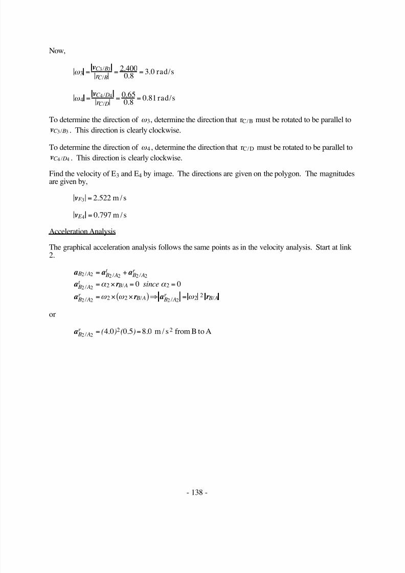
7/17/2019 Chapter 2. Graphical Position Velocity ...
http://slidepdf.com/reader/full/chapter-2-graphical-position-velocity- 91/118
- 138 -
Now,
ω 33 3 2 400
0 83 0= = =
vC B
C Br /
/
..
. rad/s
ω 4
4 4 0 650 8 0 81= = =
vC D
C Dr
/
/
.. . rad/s
To determine the direction of ω 3, determine the direction that rC B/ must be rotated to be parallel to
vC B3 3 / . This direction is clearly clockwise.
To determine the direction of ω 4 , determine the direction that rC D/ must be rotated to be parallel to
vC D4 4 / . This direction is clearly clockwise.
Find the velocity of E3 and E4 by image. The directions are given on the polygon. The magnitudesare given by,
v E 3 2 522=
. m / s
v E 4 0 797= . m / s
Acceleration Analysis
The graphical acceleration analysis follows the same points as in the velocity analysis. Start at link2.
a a a
a r
a r a r
B A B At
B Ar
B At
B A
B A
r B A
B A
r B A
ce
2 2 2 2 2 2
2 2
2 2 2 2
2 2
2 2 2 2
0 0
/ / /
/ /
/ /
/ /
sin
= +
= × = =
= × ×( ) ⇒ =
α α
ω ω ω
or
a B Ar
2 24 0 0 5 8 02
/ ( . ) ( . ) .= = m / s from B to A2

7/17/2019 Chapter 2. Graphical Position Velocity ...
http://slidepdf.com/reader/full/chapter-2-graphical-position-velocity- 92/118
- 139 -
1 m/s
Velocity Scale
C
B
D
2
34
E
b
oo'
1aB 2 / A2
r
1aC
3/ B
3
t
c3
3
e3
e4
4 m/s
AccelerationScale
d'4
1aE4
2
A
e'3
e'4
c'3
1aC3 / B3
r 1aE3
b'3
1aC
4/D
4
r1a
C4 /D4
t
1aC3

7/17/2019 Chapter 2. Graphical Position Velocity ...
http://slidepdf.com/reader/full/chapter-2-graphical-position-velocity- 93/118
- 140 -
Now go to Point C and follow the same path as was used with velocities.
a a a r vC D C Dt
C Dr
C D C D4 4 4 4 4 4 4 44 4 / / / / / = + = × + ×α ω
Also
a a a a a a
r v a
C D C B B A C Bt
C Br
B A
C B C B B A
4 4 3 3 2 2 3 3 3 3 2 2
3 3 2 23 3
/ / / / / /
/ / /
= + = + +
= × + × +α ω
Therefore,
a a a a aC Dt
C Dr
C Bt
C Br
B A4 4 4 4 3 3 3 3 2 2 / / / / / + = + +
and
a vC D
r
C D4 4 4 44 0 812 0 650 0 528 / / ( . )( . ) .= × = =
[ ]ω
from C to D
a r r C Dt
C D C D4 4 4 / / / ?= × = ⊥α
a vC Br
C B3 3 3 33 3 0 2 4 7 2 / / ( . )( . ) .= × = =[ ]ω from C to B
a r r C Bt
C B C B3 3 3 / / / ?= × = ⊥α
These values permit us to solve for the unknown vectors. We can then find “e” by accelerationimage. From the acceleration polygon,
aC B
t 3 3 16 13 / .
=m / s
2
Then,
α 33 3 16 13
0 820 16= = =
a
r C Bt
C B
/
/
.
. . rad/s2
To determine the direction of α 3 , determine the direction that r C B/ must be rotated to be parallel to
aC Bt
3 3 / . This direction is clearly counterclockwise.
and
a E 315 84= . m / s2
a E 432 19= . m / s2

7/17/2019 Chapter 2. Graphical Position Velocity ...
http://slidepdf.com/reader/full/chapter-2-graphical-position-velocity- 94/118
- 141 -
Problem 2.33
In the mechanism shown, point A lies on the X axis. Draw the basic velocity and accelerationpolygons and use the image technique to determine the velocity and acceleration of point D4. Thendetermine the velocity and acceleration images of link 4. Draw the images on the velocity andacceleration polygons.
A
B D
E
F (-1.0", -0.75")
2
3
4
5
6
v = 10 in/sA2
(constant)
C X
Y
FE = 1.35" ED = 1.5" BD = CD = 1.0" AB = 3.0"
84˚
90˚
Square
Position Analysis:
Plot the linkage to scale. Start by drawing point D and the rest of link 4. Next draw link B andfinally draw link 3. Links 5 and 6 do not need to be drawn because they do not affect theinformation that is requested.
Velocity Analysis:
v v A A3 2=
v v B B3 4=
v v v v v B A B A B B C 3 3 3 3 4 4 4= + = = / / (1)
Now,
v A2 10= in / s in the horizontal direction
v v r v r r B B B C B B C B C 3 4 4 4 44 4= = × ⇒ = ⋅ ⊥ω ω / / / ( )to
v r v r r B A B A B A B A B A3 3 3 3 3 33 3 / / / / / ( )= × ⇒ = ⊥ω ω to

7/17/2019 Chapter 2. Graphical Position Velocity ...
http://slidepdf.com/reader/full/chapter-2-graphical-position-velocity- 95/118
- 142 -
30 in/s
Acceleration Scale
2
A
B
C
D
5 in/s
Velocity Scale
a3o
b3
c4
b4
d4
1aB3/A3r
1aB 4/C4
r
b3'
o'
a'2a'3c'4
1a B3/A3t
1a B4 /C 4
t
b4'
d4'
Solve Eq. (1) graphically with a velocity polygon. From the polygon,
v B A3 3 6 64 / .= in/s
or

7/17/2019 Chapter 2. Graphical Position Velocity ...
http://slidepdf.com/reader/full/chapter-2-graphical-position-velocity- 96/118
- 143 -
ω 33 3 6 64
32 21= = =
v
r B A
B A
/
/
. . rad/s
To determine the direction of ω 3, determine the direction that r B A/ must be rotated to be parallel to
v B A3 3 / . This direction is clearly counterclockwise.
Also,
v B4 9 70= . in/s
and
ω 44 4 9 70
1 4146 86= = =
v
r B C
B C
/
/
..
. rad/s
To determine the direction of ω 4 , determine the direction that r B C / must be rotated to be parallel to
v B C 4 4 / . This direction is clearly clockwise.
Also,
v r D D C 4 6 77= ⊥. ( ) / in / s to
Draw the image of link 4 on the velocity polygon. The image is a square.
Acceleration Analysis:
a a A A2 3=
a a a a a B B A B A B C 3 4 3 3 3 4 4= = + = / /
a a a a a B C r
B C t
A B Ar
B At
4 4 4 4 3 3 3 3 3 / / / / + = + +(3)
Now,
a A3 0=
a r a r B C r
B C B C r
B C 4 4 4 44 4 42 26 86 1 414 66 54 / / / / . . .= × ×( ) ⇒ = ⋅ = ⋅ =ω ω ω in/s2
in the direction of - r B C /
a r a r r B C t
B C B C t
B C B C 4 4 4 44 4 / / / / / ( )= × ⇒ = ⋅ ⊥α α to
a r a r B Ar
B A B Ar
B A3 3 3 33 3 32 22 21 3 14 6 / / / / . .= × ×( ) ⇒ = ⋅ = ⋅ =ω ω ω in /s2
in the direction of - r B A/
a r a r r B At
B A B At
B A B A3 3 3 3 3 33 3 / / / / / ( )= × ⇒ = ⋅ ⊥α α to

7/17/2019 Chapter 2. Graphical Position Velocity ...
http://slidepdf.com/reader/full/chapter-2-graphical-position-velocity- 97/118
- 144 -
Solve Eq. (3) graphically with a acceleration polygon. From the polygon,
a D4 54 0= . in/s2
The image of link 4 is a square as shown on the acceleration polygon.
Problem 2.34
In the mechanism shown below, the velocity of A2 is 10 in/s to the right and is constant. Draw thevelocity and acceleration polygons for the mechanism, and record values for angular velocity andacceleration of link 6. Use the image technique to determine the velocity of points D3, and E 3, andlocate the point in link 3 that has zero velocity.
AC
B D
E
F 2
34
5
6v = 10 in/sA2
(constant)
CF = 1.95"FE = 1.45" ED = 1.5"CD = 1.0"
BC = 1.45" BD = 1.05" AB = 3.0"
103˚
Position Analysis:
Locate points C and F and the line of action of A. Draw link 6 and locate pont E. Then locate pointD. Next locate point B and finally locate point A.
Velocity Analysis:
The equations required for the velocity analysis are:
v v A A3 2=
v v B B3 4=
v v v B A B A3 3 3 3= + / (1)
v v D D5 4=
v v v v E E D E D5 6 5 5 5= = + / (2)
Now,
v A2 10= in/s in the horizontal direction

7/17/2019 Chapter 2. Graphical Position Velocity ...
http://slidepdf.com/reader/full/chapter-2-graphical-position-velocity- 98/118
- 145 -
v v r v r r B B B C B B C B C 3 4 44 4= = × ⇒ = ⋅ ⊥ω ω / / / ( )to
v r v r r B A B A B A B A B A3 3 3 33 3 / / / / / ( )= × ⇒ = ⊥ω ω to
Solve Eq. (1) graphically with a velocity polygon. From the polygon,
v B A3 3 5 97 / .= in/s
ω 33 3 5 97
31 99= = =
v
r B A
B A
/
/
. . rad/s
Also,
v B in s4 9 42= . /
or
ω 4
4 4
4 4
9 421 45 6 50= = =
v
r
B C
B C
/
/
.
. . rad/sCW
Now,
v r D D C in s to4 6 50= ⊥. / ( ) /
v r v r r E D E D E D E D E D5 5 5 55 5 / / / / / ( )= × ⇒ = ⊥ω ω to
v v v r v r r E E E F E F E F E F E F 5 6 6 6 6 66 6= = = × ⇒ = ⊥ / / / / / ( )ω ω to
Solve Eq. (2) graphically with a velocity polygon. From the polygon,
v E 6 5 76= . in/s
or
ω 66 6 5 76
1 453 97= = =
v
r E F
E F
/
/
.
. . rad/s
Acceleration Analysis:
a a A A2 3=
a a a a B B A B A3 4 3 3 3= = + /
a a a a B C r
B C t
B Ar
B At
4 4 4 4 3 3 3 3 / / / / + = +(3)
a a D D5 4=
a a a a a E E E F D E D5 6 6 6 5 5 5= = = + / /

7/17/2019 Chapter 2. Graphical Position Velocity ...
http://slidepdf.com/reader/full/chapter-2-graphical-position-velocity- 99/118
- 146 -
a a a a a E F r
E F t
D E Dr
E Dt
6 6 6 6 5 5 5 5 5 / / / / + = + +(4)
Now,
A C
B
D
E
F2
34
6
o'
25 in/s
Acceleration Polygon
2
1aB3 /A3
r
1aB3/A3
t
1 aB4 /C 4
r
b3’ b4b’,
d4'
1aE5/ D 5r
1aE5/D 5
t
1aE6 /F6
r
e5'
1aB4/ C4t
1 aE6 /F6
t
O2.5 in/s
Velocity Polygon
a2
a3
,
b3 b4b,
d4 d5,
e5
3
o
d3
e3
5D
or
a r a r B C r
B C B C r
B C 4 4 4 44 4 42 26 50 1 45 61 3 / / / / . . .= × ×( ) ⇒ = ⋅ = ⋅ =ω ω ω in/s2
in the direction of - r B C /
a r a r r B C t
B C B C t
B C B C 4 4 4 44 4 / / / / / ( )= × ⇒ = ⋅ ⊥α α to

7/17/2019 Chapter 2. Graphical Position Velocity ...
http://slidepdf.com/reader/full/chapter-2-graphical-position-velocity- 100/118
- 147 -
a r a r B Ar
B A B Ar
B A3 3 3 33 3 32 21 99 3 11 9 / / / / . .= × ×( ) ⇒ = ⋅ = ⋅ =ω ω ω in /s2
in the direction of - rB A/
a r a r r B At
B A B At
B A B A3 3 3 33 3 / / / / / ( )= × ⇒ = ⋅ ⊥α α to
Solve Eq. (3) graphically with an acceleration polygon. From the polygon,
a B At
3 365 3 / .= in/s2
or
α 323 3 65 3
321 8= = =
a
r B At
B Arad s CW
/
/
. . /
And,
a D3 86 6= . in/s2
Also,
a r a r E Dr
E D E Dr
E D5 5 5 55 5 52 21 73 1 5 4 49 / / / / . . .= × ×( ) ⇒ = ⋅ = ⋅ =ω ω ω in/s2
in the direction of - r E D/
a r a r r E Dt
E D E Dt
E D E D5 5 5 55 5 / / / / / ( )= × ⇒ = ⋅ ⊥α α to
a r a r E F r
E F E F r
E F 6 6 6 66 6 62
25 76 1 45 48 1 / / / / . . .= × ×( ) ⇒ = ⋅ = ⋅ =ω ω ω in/s2
in the direction of - r E F /
a r a r r E F t
E F E F t
E F E F 6 6 6 66 6 / / / / / ( )= × ⇒ = ⋅ ⊥α α to
Now solve Eq. (4) using the acceleration polygon. Then,
a E F t
6 638 2 / .= in/s2
or
α 66 6 38 2
1 4526 4= = =
a
r E F t
E F
/
/
..
. rad / s CCW2
Using the image concept, the velocities of points D3 and E3 are
v D3 10 2= . in/s

7/17/2019 Chapter 2. Graphical Position Velocity ...
http://slidepdf.com/reader/full/chapter-2-graphical-position-velocity- 101/118
- 148 -
v E 3 12 7= . in/s
The point in link 3 with zero velocity is shown on position diagram. The point is found by finding
the position image of oa b3 3.
Problem 2.35
The instant center of acceleration of a link can be defined as that point in the link that has zeroacceleration. If the accelerations of Points A and B are as given in the rigid body shown below, findthe Point C in that link at which the acceleration is zero.
B
A
Aa
aB
70˚
5˚
145˚
Aa = 1500 in/s2
= 1050 in/saB2
AB = 3.75"
Acceleration Analysis:
Draw the accelerations of points A and B on an acceleration polygon. Then o' will correspond tothe instant center of acceleration. Find the image of o' on the position diagram, and that will be thelocation of C

7/17/2019 Chapter 2. Graphical Position Velocity ...
http://slidepdf.com/reader/full/chapter-2-graphical-position-velocity- 102/118
- 149 -
500 in/s
Acceleration Scale
2
o'
a'
b'
c'
A
B
C
1 in
Problem 2.36
The following are given for the mechanism shown in the figure:
ω α 2 26 5 40= =. rad/ s (CCW); rad/ s (CCW)2
Draw the velocity polygon, and locate the velocity of Point E using the image technique.
A
C
B
D (2.2", 1.1")
2
34
E
55˚
X
Y
AB = DE = 1.0 in BC = 2.0 inCD = 1.5 in
Position Analysis
Locate the two pivots A and D. Draw link 2 and locate pivot B. Then find point C and finallylocate E.
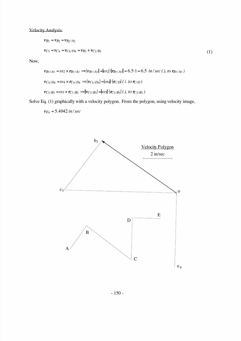
7/17/2019 Chapter 2. Graphical Position Velocity ...
http://slidepdf.com/reader/full/chapter-2-graphical-position-velocity- 103/118
- 150 -
Velocity Analysis:
v v v B B B A3 2 2 2= = /
v v v v vC C C D B C B3 4 4 4 3 3 3= = = + / / (1)
Now,
v r v r r B A B A B A B A B Ain to2 2 2 2 2 2 2 2 2 22 2 6 5 1 6 5 / / / / / . . / sec ( )= × ⇒ = ⋅ = ⋅ = ⊥ω ω
v r v r r C D C D C D C D C Dto4 4 4 4 4 44 4 / / / / / ( )= × ⇒ = ⋅ ⊥ω ω
v r v r r C B C B C B C B C Bto3 3 3 3 3 3 3 3 3 33 3 / / / / / ( )= × ⇒ = ⋅ ⊥ω ω
Solve Eq. (1) graphically with a velocity polygon. From the polygon, using velocity image,
v E in4 5 4042= . / sec
c3
b3
o
2 in/sec
Velocity Polygon
e4
A
C
B
D
E

7/17/2019 Chapter 2. Graphical Position Velocity ...
http://slidepdf.com/reader/full/chapter-2-graphical-position-velocity- 104/118
- 151 -
Problem 2.37
In the mechanism shown, find ωω ω ω 6 and αα α α 3. Also, determine the acceleration of D3 by image.
AC
B
D
E
F (-1.0", -0.75")
2
3 4
5
6
v = 10 in/sA2(constant)
X
Y
81˚
CD = 1.0"BD = 1.05"BC = 1.45"ED = 1.5"FE = 1.4"AB = 3.0"
Velocity Analysis:
v v A A3 2=
v v B B3 4=
v v v B A B A3 3 3 3= + / (1)
v v D D5 4=
v v v v E E D E D5 6 5 5 5= = + / (2)
Now,
v A in2 10= /sec in the horizontal direction
v v r v r r B B B C B B C B C to3 4 4 4 4 4 4 4 44 4= = × ⇒ = ⋅ ⊥ω ω / / / ( )
v r v r r B A B A B A B A B Ato3 3 3 3 3 3 3 3 3 33 3 / / / / / ( )= × ⇒ = ⊥ω ω
Solve Eq. (1) graphically with a velocity polygon. From the polygon,
v B A in3 3 6 282 / . / sec=
or
ω 33 3
3 3
6 2823
2 094= = =v
r
B A
B A
rad /
/
. . / sec

7/17/2019 Chapter 2. Graphical Position Velocity ...
http://slidepdf.com/reader/full/chapter-2-graphical-position-velocity- 105/118
- 152 -
AC
B
D
E
F
3
45
62
d4 d5,
2.5 in/sec
Velocity Polygon
o
b3 b4b,
a2 a3,
e5
25 in/sec
Acceleration Polygon
2o'1a B3 /A3
r
1aB3 / A3
t
1aB4/C4
t
1aB4/C4r
b3’ b4b’,
d3'
Also,
v B in4 9 551= . / sec
or
ω 44 4
4 4
9 5511 45
6 587= = =v
r B C
B C rad CW
/
/
..
. / sec
Now,
v D in4 6 587= . / sec ( )/⊥ to D Cr 4 4

7/17/2019 Chapter 2. Graphical Position Velocity ...
http://slidepdf.com/reader/full/chapter-2-graphical-position-velocity- 106/118
- 153 -
v r v r r E D E D E D E D E Dto5 5 5 5 5 5 5 5 5 55 5 / / / / / ( )= × ⇒ = ⊥ω ω
v v v r v r r E E E F E F E F E F E F to5 6 6 6 6 6 6 6 6 6 6 66 6= = = × ⇒ = ⊥ / / / / / ( )ω ω
Solve Eq. (2) graphically with a velocity polygon. From the polygon,
v E in6 6 132= . / sec
or
ω 66 6
6 6
6 1321 45
4 229= = =v
r E F
E F rad CW
/
/
..
. / sec
Acceleration Analysis:
a a A A2 3=
a a a a B B A B A3 4 3 3 3= = + /
a a a a B C r
B C t
B Ar
B At
4 4 4 4 3 3 3 3 / / / / + = +(3)
Now,
a r a r B C r
B C B C r
B C in4 4 4 4 4 4 4 44 4 4
2 2 26 587 1 45 62 913 / / / / . . . / sec= × ×( ) ⇒ = ⋅ = ⋅ =ω ω ω
in the direction ofrB C4 4/
a r a r B C t
B C B C t
B C 4 4 4 4 4 4 4 44 4 / / / / = × ⇒ = ⋅α α ( ) / ⊥ to B C r 4 4
a r a r B Ar
B A B Ar
B A in3 3 3 3 3 33 3 3
2 2 22 094 3 13 155 / / / / . . / sec= × ×( ) ⇒ = ⋅ = ⋅ =ω ω ω
in the direction of rB A/
a r a r r B At
B A B At
B A B Ato3 3 3 3 3 3 3 3 3 33 3 / / / / / ( )= × ⇒ = ⋅ ⊥α α
Solve Eq. (3) graphically with a acceleration polygon. From the polygon,
a B At in
3 368 568 2
/ . / sec=
or
α 323 3
3 3
68 5683
22 856= = =a
r B At
B Arad CW
/
/
. . / sec
Also,
a D in3 91 390 2= . / sec

7/17/2019 Chapter 2. Graphical Position Velocity ...
http://slidepdf.com/reader/full/chapter-2-graphical-position-velocity- 107/118
- 154 -
Problem 2.38
In the mechanism shown, ωω ω ω 2 = 1 rad/s (CCW) and αα α α 2 = 0 rad/s2. Find ωω ω ω 5, αα α α 5, vE6, aE6 for the
position given. Also find the point in link 5 that has zero acceleration for the position given.
A
C
B
D
2
3
4 E 5
6
30˚
AD = 1 m AB = 0.5 m BC = 0.8 mCD = 0.8 m BE = 0.67 m
0.52 m
Velocity Analysis
v v v v B B B B A2 3 5 2 2= = = /
v v v v E E B E B5 6 5 5 5= = + / (1)
Now,
v r v r r B A B A B A B A B Am to2 2 2 2 2 2 2 2 2 22 2 1 0 5 0 5 / / / / / . . / sec ( )= × ⇒ = ⋅ = ⋅ = ⊥ω ω
15vE in the horizontal direction
v r v r r E B E B E B E B E Bto5 5 5 5 5 5 5 5 5 55 5 / / / / / ( )= × ⇒ = ⋅ ⊥ω ω
Solve Eq. (1) graphically with a velocity polygon. From the polygon,
v E B m5 5 0 47313 / . / sec=
or
ω 55 5
5 5
0 473130 67
0 706= = =v
r E B
E Brad CCW
/
/
..
. / sec
Also,

7/17/2019 Chapter 2. Graphical Position Velocity ...
http://slidepdf.com/reader/full/chapter-2-graphical-position-velocity- 108/118
- 155 -
A
C
B
D
2
3
4
E5
6
o'
0.1 m/sec
Acceleration Polygon2
1 aE5
1aB2/A2
r
1a E5/B5
r
1aE5 /B 5
tb3b'
e5'
2.2°
27.8°
O'
0.1 m/sec
Velocity Polygon
b5
o
e 5
v E m6 0 441= . / sec
Acceleration Analysis:
a a a a B B B B A2 3 5 2 2= = =
/
a a a a E E B E B5 6 5 5 5= = + /
a a a a a E B Ar
B At
E Br
E Bt
5 2 2 2 2 5 5 5 5= + + + / / / / (2)
Now,

7/17/2019 Chapter 2. Graphical Position Velocity ...
http://slidepdf.com/reader/full/chapter-2-graphical-position-velocity- 109/118
- 156 -
a E 5 in horizontal direction
a r a r B Ar
B A B Ar
B A m2 2 2 22 2 2
2 2 21 0 5 0 5 / / / / . . / sec= × ×( ) ⇒ = ⋅ = ⋅ =ω ω ω
in the direction opposite to rB A/
a r a r B At
B A B At
B A m2 2 2 22 2
20 1 0 / / / / /sec= × ⇒ = ⋅ = ⋅ =α α
a r a r E Br
E B E Br
E B m5 5 5 55 5 5
2 2 20 706 0 67 0 334 / / / / . . . / sec= × ×( ) ⇒ = ⋅ = ⋅ =ω ω ω
in the direction opposite to rE B/
a r a r r E Bt
E B E Bt
E B E Bto5 5 5 55 5 / / / / / ( )= × ⇒ = ⋅ ⊥α α
Solve Eq. (2) graphically with an acceleration polygon. From the polygon,
a E m6 0 042 2= . / sec
Also,
a E Bt m
5 50 42 2
/ . / sec=
or
α 525 5
5 5
0 420 67
0 626= = =a
r E Bt
E Brad CW
/
/
.
. . / sec
Using acceleration image, point O' is in the location in which the acceleration of link five is zero.

7/17/2019 Chapter 2. Graphical Position Velocity ...
http://slidepdf.com/reader/full/chapter-2-graphical-position-velocity- 110/118
- 157 -
Problem 2.39
Part of an eight-link mechanism is shown in the figure. Links 7 and 8 are drawn to scale, and the
velocity and acceleration of point D7 are given. Find ωω ω ω 7 and αα α α 7 for the position given. Also find
the velocity of G7 by image.
D
E
7
6
G
8
X
Y
1.25"1.6"
DE = 1.5" DG = 0.7"GE = 1.65"
= 5.0 320˚ in/sec = 40 260˚ in/s 2vD7 aD7
Velocity Analysis
Compute the velocity of Points E7 and E8.
v v
v v v E E E D E D
7 87 7 7 7
=
= + /
and because points on the same link are involved,
v v v r v D E D D E D E 7 7 7 7 87+ = + × = / / ω
From the velocity polygon:
v E in8 2 884= . / sec
in the direction shown, and
v E D in7 7 3 405 / . / sec=
in the direction shown.
ω 77 7 3 405
1 502 27= = =
v
r E D
E Drad
/
/
..
. / sec
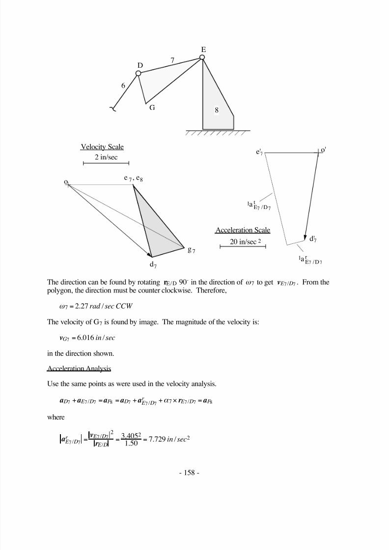
7/17/2019 Chapter 2. Graphical Position Velocity ...
http://slidepdf.com/reader/full/chapter-2-graphical-position-velocity- 111/118
- 158 -
o'
D
E
7
7d'
6
G 8
1a E7 /D7r
1a E7 /D7
t
e'72 in/sec
Velocity Scale
220 in/sec
Acceleration Scale
7d
7e 8, e
7g
o
The direction can be found by rotating rE D/ 90˚ in the direction of ω 7 to get v E D7 7 / . From the
polygon, the direction must be counter clockwise. Therefore,
ω 7 2 27= . / secrad CCW
The velocity of G7 is found by image. The magnitude of the velocity is:
vG in7 6 016= . / sec
in the direction shown.
Acceleration Analysis
Use the same points as were used in the velocity analysis.
a a a a a r a D E D F D E Dr
E D F 7 7 7 8 7 7 7 7 7 87+ = = + + × = / / / α
where
a v
r E Dr E D
E Din
7 77 7
2 223 405
1 507 729 /
/
/
..
. / sec= = =

7/17/2019 Chapter 2. Graphical Position Velocity ...
http://slidepdf.com/reader/full/chapter-2-graphical-position-velocity- 112/118
- 159 -
in the direction opposite rE D/ .
From the polygon,
a r E Dt
E D7 7 7 77 0 / / = × =α
Therefore,
α 727 7 42 59
1 5028 40= = =
a
r E Dt
E Drad
/
/
..
. / sec
The direction can be found by rotating rE D/ 90˚ in the direction of ω 7 to get a E Dt
7 7 / . From the
polygon, the direction must be counter clockwise. Therefore,
a7 228 40= . / secrad CCW
Problem 2.40
In the mechanism shown below, link 2 is rotating CW at the rate of 3 rad/s (constant). In theposition shown, link 2 is horizontal. Write the appropriate vector equations, solve them using vectorpolygons, and
a) Determine vC4, vE4
, ωω ω ω 3, and ωω ω ω 4.
b) Determine aC4, aE4
, αα α α 3, and αα α α 4.
Link lengths: AB = 3 in, BC = BE = CE = 5 in, CD = 3 in
B
C
2
3
4
D
ω 2
A
7"
E
Position Analysis
Draw the linkage to scale. Start by locating the relative positions of A and D. Next locate B andthen C. Then locate G.
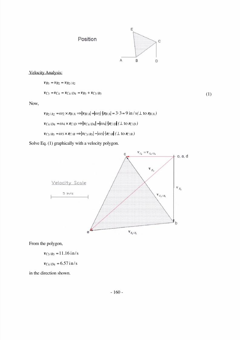
7/17/2019 Chapter 2. Graphical Position Velocity ...
http://slidepdf.com/reader/full/chapter-2-graphical-position-velocity- 113/118
- 160 -
Velocity Analysis:
v v v B B B A3 2 2 2= = /
v v v v vC C C D B C B3 4 4 4 3 3 3= = = + / / (1)
Now,
v r v r r B A B A B A B A B A2 2 2 2 3 3 9 / / / / / ( )= × ⇒ = ⋅ = ⋅ = ⊥ω ω in / s to
v r v r r C D C D C D C D C D4 4 4 44 4 / / / / / ( )= × ⇒ = ⋅ ⊥ω ω to
v r v r r C B C B C B C B C B3 3 3 33 3 / / / / / ( )= × ⇒ = ⋅ ⊥ω ω to
Solve Eq. (1) graphically with a velocity polygon.
From the polygon,
vC B3 3 11 16 / .= in/s
vC D4 4 6 57 / .= in /s
in the direction shown.
7/17/2019 Chapter 2. Graphical Position Velocity ...
http://slidepdf.com/reader/full/chapter-2-graphical-position-velocity- 114/118
- 161 -
Now
ω 33 3 11 16
52 232= = =
v
r C B
C B
/
/
. . rad/s
and
ω 44 4 6 57
32 19= = =
v
r C D
C D
/
/
. . rad/s
To determine the direction of ω 3, determine the direction that r C B/ must be rotated to be parallel to
vC B3 3 / . This direction is clearly clockwise.
To determine the direction of ω 4 , determine the direction that r C D/ must be rotated to be parallel to
vC D4 4 / . This direction is clearly counterclockwise.
The velocity of point E3
v v v v r E B E B B E B3 3 3 3 3 3= + = + × / / ω
from the polygon
v E 3 13 5= . in/s
vC 4 6 57= . in/s
Acceleration Analysis:
a a a B B B A3 2 2 2= = /
a a a a aC C C D B C B3 4 4 4 3 3 3= = = + / /
a a a a a aC Dr
C Dt
B Ar
B At
C Br
C Bt
4 4 4 4 2 2 2 2 3 3 3 3 / / / / / / + = + + +(2)
Now,
a r a r B Ar
B A B Ar
B A2 2 2 22 2 22 23 3 27 / / / / = × ×( ) ⇒ = ⋅ = ⋅ =ω ω ω in/s2
in the direction of - r B A2 2/
a r a r B At B A B At B A2 2 2 22 2 0 / / / / = × ⇒ = =α α
a r a r C Br
C B C Br
C B3 3 3 33 3 32 22 232 5 24 9 / / / / . .= × ×( ) ⇒ = ⋅ = ⋅ =ω ω ω in /s2
in the direction of - r C B/
a r a r r C Bt
C B C Bt
C B C B3 3 3 33 3 / / / / / ( )= × ⇒ = ⋅ ⊥α α to

7/17/2019 Chapter 2. Graphical Position Velocity ...
http://slidepdf.com/reader/full/chapter-2-graphical-position-velocity- 115/118
- 162 -
a r a r C Dr
C D C Dr
C D in4 4 4 44 4 4
2 2 22 19 3 14 39 / / / / . . / sec= × ×( ) ⇒ = ⋅ = ⋅ =ω ω ω
in the direction of - rC D/
a r a r r C Dt
C D C Dt
C D C Dto4 4 4 44 4 / / / / / ( )= × ⇒ = ⋅ ⊥α α
Solve Eq. (2) graphically with acceleration.
From the acceleration polygon,
aC Bt 3 3 0 / = in/s2
aC Dt
4 446 71 / .= in/s2
Then,
α 33 3 0
20= = =
a
r C Bt
C B
/
/ rad/s2
α 44 4 46 71
315 57= = =
a
r C Dt
C D
/
/
. . rad/s2
To determine the direction of α 4, determine the direction that r C D/ must be rotated to be parallel to
aC Dt
4 4 / . This direction is clearly counterclockwise.
Determine the acceleration of point E3
a a a a a a E B E B B E Br
E Bt
3 3 3 3 2 3 3 3 3= + = + + / / /

7/17/2019 Chapter 2. Graphical Position Velocity ...
http://slidepdf.com/reader/full/chapter-2-graphical-position-velocity- 116/118
- 163 -
a r a r E Bt
E B E Bt
E B in3 3 3 33 3
20 1 0 / / / / /sec= × ⇒ = ⋅ = ⋅ =α α
a r a r E Br
E B E Br
E B in3 3 3 33 3 3
2 2 22 232 5 24 9 / / / / . . / sec= × ×( ) ⇒ = ⋅ = ⋅ =ω ω ω
From the acceleration polygon,
a E 3 34 29= . in/s2
aC 4 48 87= . in/s2
Problem 2.41
Part of a 10-link mechanism is shown in the figure. Links 7 and 8 are drawn to scale, and the
velocity and acceleration of points D7 and F 8 are given. Find ωω ω ω 8 and αα α α 7 for the position given.
Also find the velocity of G7 by image.
D
E
F (1.8", -1.05")
7
8
9
6
G
X
Y
DE = 1.5" EF = 1.45" DG = 0.7" EG = 1.65"
= 6.0 353˚ in/s
= 7.5 54˚ in/s
= 40 235˚ in/s 2
= 30 305˚ in/s 2
v D
vF
7
8
aD
a F
7
8
Velocity Analysis
Compute the velocity of Points E7 and E8.
v v
v v vv v v
E E
E D E D E F E F
7 8
7 7 7 7
8 8 8 8
=
= +
= + /
/
Therefore,
v v v v D E D F E F 7 7 7 8 8 8+ = + / /
and because points on the same link are involved,

7/17/2019 Chapter 2. Graphical Position Velocity ...
http://slidepdf.com/reader/full/chapter-2-graphical-position-velocity- 117/118
- 164 -
v v v v v r v r D E D F E F D E D F E F 7 7 7 8 8 8 7 7 7 8 8 87 8+ = + = + × = + × / / / / ω ω
From the velocity polygon:
v E F 8 8 0 / =
so
ω 8 0=
The velocity of G7 is found by image. The magnitude of the velocity is
vG7 9 1= . in/s
o'
o
7d
E
7d'
8f
8f'
D
F
7
8
9
6
G
8e,
7g
7e,
8e' 7e',
5 in/s
Velocity Polygon
220 in/s
Velocity Polygon
vG7
9 1= . in/s
Acceleration Analysis
Use the same points as were used in the velocity analysis for the acceleration analysis.
a a a a
a a r a a r
D E D F E F
D E Dr
E D F E F r
E F
7 7 7 8 8 8
7 7 7 7 7 8 8 8 8 87 8
+ = +
= + + × = + + ×
/ /
/ / / / α α

7/17/2019 Chapter 2. Graphical Position Velocity ...
http://slidepdf.com/reader/full/chapter-2-graphical-position-velocity- 118/118
a v
r
a v
r
E Dr E D
E D
E F r E F
E F
7 7
7 7
7 7
8 8
8 8
8 8
2 2
2 2
6 921 50
32 0
01 44
0
/ /
/
/ /
/
..
.
.
= = =
= = =
in/s
in/s
2
2
From the polygon,
a r E Dt
E D7 7 7 77 0 / / = × =α
Therefore,
α 7 0=