chapter 16 adaptive polarization design for target ... 16_gini_chapter16.tex march 19, 2012 11: 0...
TRANSCRIPT

Gini 16_Gini_Chapter16.tex March 19, 2012 11: 0 Page 453
Chapter 16
Adaptive polarization design for target detectionand tracking
Martin Hurtado1,∗, Sandeep Gogineni2 and Arye Nehorai2
Abstract
Transmitting waveforms with different polarizations in radar systems provide morecomplete information about the target and its environment, ensuring a significantenhancement of the radar’s performance. Conventional polarimetric radars transmitwaveforms with a fixed polarization pattern, independent of the target and cluttercharacteristics. In this chapter, we explore the adaptive design of radar polariza-tion waveforms. We focus on a closed-loop system that sequentially estimates thetarget and clutter scattering parameters and then uses these estimates to select thepolarization of the subsequent waveforms. We demonstrate that the radar system per-formance is significantly improved when the polarization of the transmitted signalis optimally and adaptively selected to match the polarimetric aspects of the targetand the environment. In particular, we include an overview of our recent results inpolarimetric design for radar detection and tracking.
Keywords: Polarimetric radar; mono-static radar; MIMO radar; detection; tracking;adaptive design.
16.1 Introduction
Radar systems transmit electromagnetic (EM) waves, collect their returns and pro-cess the recorded data to acquire information of a remote target or scene. Theorientation of the oscillations of the electric and magnetic fields in the plane per-pendicular to direction of travel is called polarization. Multiple polarization states
1 Department of Electrical Engineering, National University of La Plata, Argentina2 Department of Electrical and Systems Engineering, Washington University in St. Louis, One BrookingsDrive, St. Louis, MO 63130, USA∗ Previously, Martin Hurtado was with the Department of Electrical and Systems Engineering, WashingtonUniversity in St. Louis, One Brookings Drive, St. Louis, MO 63130, USA

Gini 16_Gini_Chapter16.tex March 19, 2012 11: 0 Page 454
454 Waveform design and diversity for advanced radar systems
of an EM signal enable it to capture multiple-copy information of a target, whichresults in so-called polarization diversity. Polarimetric diversity has become an impor-tant tool for detecting and tracking targets of small radar cross-sections. Unlikeconventional radar systems, which operate with identically polarized antennas fortransmission and reception, polarimetric radar transmits and receives waveforms withdifferent polarizations, leading to the compatibility of acquiring complete polarimetricinformation of the target and the environment. Polarization provides more completeinformation about the target/environment features, such as the geometry, materialand orientation. Exploiting polarimetric information can greatly enhance radar capa-bilities, particularly when the usual signal descriptors, such as time, frequency andbearing, are not sufficient for discriminating the target from the clutter/environment.
The effort of applying polarization diversity to enhance the radar performancecan be traced back to the 1950s (see References 1, 2 and the references therein).In Reference 3, Sinclair formulated a model to characterize an antenna when trans-mitting a polarized wave and calculated the voltage at the sensor output whenreceiving waves of any arbitrary polarization. In Reference 4, Kennaugh demonstratedthat there exist signal polarization states for which the radar receives maximumpower. This idea of optimal polarization was later extended by Huynen [5]. In Ref-erence 6, Ioannidis and Hammers proposed a method for selecting the optimumantenna polarizations for discriminating targets in the presence of clutter. In morerecent work, Novak et al. [7,8] derived the optimal polarimetric detector. Moreover,they extended the use of product models to the full polarimetric case to account for theeffects of non-homogeneous clutter. Several authors have demonstrated that polariza-tion can enhance the radar resolution when jointly processed with other signal features,such as bearing, frequency or code [9–13]. The problem of polarimetric waveformdesign for improving the target detection and identification is addressed in Refer-ence 14. Most of the existing literature about polarization diversity explores theperformance of radar systems that transmit waveforms with a fixed polarizationpattern (e.g. alternating between H and V polarized signals).
In this chapter, we demonstrate that the detection and tracking performances ofradar systems are significantly improved when the polarization of the transmittedsignal is optimally and adaptively selected to match the polarimetric aspects of thetarget and the environment. We provide an overview of our recent results showingthat the adaptive design of the radar signal polarization enables achieving optimalperformance in several operating modes [15–18]. In particular, we discuss threeproblems related to polarimetric waveform design.
We first discuss the problem of polarized waveform design for optimal targetdetection. We present a detection test statistic with a closed-form expression thatincorporates information about the estimated polarimetric aspects of the target andthe clutter. The analysis of the detection performance is used to adaptively schedulethe next transmission polarization to enhance the target detection. We select the signalpolarization that maximizes the non-centrality parameter of the detection statisticdistribution under the assumption that the target is present [15].
Next, we examine the problem of optimal design for target detection using polari-metric multiple-input multiple-output (MIMO) radar systems with widely separated

Gini 16_Gini_Chapter16.tex March 19, 2012 11: 0 Page 455
Adaptive polarization design for target detection and tracking 455
antennas. These systems exploit spatial diversity in addition to the polarization diver-sity provided by conventional single-input single-output (SISO) polarimetric radarsystems. Each transmitter is capable of adaptively choosing the polarization of itstransmitted waveform based on the knowledge of the environment [16]. We anal-yse the performance of the detector by deriving approximate expressions for theprobabilities of detection and false alarm. Using these expressions, we choose theoptimal transmit waveform polarizations. We demonstrate significant improvementin performance due to optimal polarimetric design.
When the detection statistic exceeds the threshold, indicating the presence ofa target, the tracking system is initiated in order to sequentially estimate the tar-get parameters. Hence, we consider the problem of adaptive polarized waveformdesign for tracking targets in the presence of clutter under a framework of sequen-tial Bayesian inference. We implement the tracking algorithm using a sequentialMonte Carlo method that is suitable for non-linear and non-Gaussian state andmeasurement models. We discuss a criterion for selecting the optimal waveformpolarization one step ahead by computing a recursive form of the posterior CRB(PCRB) [17].
16.2 Target detection in heavy inhomogeneous clutter
The detection of static or slowly moving targets in heavy-clutter environments isconsidered a challenging problem, mainly because it is not possible to discriminatethe target from the clutter using the Doppler effect. Polarization diversity providesadditional information that enhances the detection of targets, particularly under theconditions described above. Detection performance could be further improved if thepolarization of the transmitted signal were optimally selected to match the targetpolarimetric aspects. In this section, we present a polarimetric detector that is robustagainst heavy inhomogeneous clutter, i.e. the detector false-alarm rate is insensitiveto changes in the clutter, while still maintaining a good probability of detection. Thetest statistic derived from the detector has a well-known distribution that depends onthe transmitted waveform parameters. Finally, we present an approach to select thesignal polarization that will maximize the target probability of detection.
16.2.1 Polarimetric radar model
We consider a mono-static radar capable of transmitting waveforms with any arbi-trary polarization on a pulse-by-pulse basis. The recorded data consist not only ofthe target echoes but also of the undesired reflections from the target environment(see Figure 16.1). We note that in order to fully identify the polarimetric aspects ofthe target and clutter, the radar dwell must consist of diversely polarized pulses. Theoutput of a diversely polarized array of Q sensors receiving the echoes from a singlerange-cell under test can be expressed as
y(t) = B(S t + Sc)ξ (t) + e(t), t = 1, . . . , N (16.1)

Gini 16_Gini_Chapter16.tex March 19, 2012 11: 0 Page 456
456 Waveform design and diversity for advanced radar systems
TargetClutter
RadarRange Cells
Clutter
Clutter
Figure 16.1 Geometry of the problem: object of interest (target) in an environment(clutter) producing undesired echoes
where
● The Q × 1 vector y(t) is the complex envelope of the measurements.● The Q × 2 matrix B is the response to the diversely polarized sensor array. If the
receiver array is a vector sensor [11], the array response is given by
B =
⎡⎢⎢⎢⎢⎢⎢⎣
− sin φ − cosφ sinψcosφ − sin φ sinψ
0 cosψ− cosφ sinψ sin φ− sin φ sinψ − cosφ
cosψ 0
⎤⎥⎥⎥⎥⎥⎥⎦
(16.2)
where φ and ψ are the azimuth and elevation angles of the cell under test,respectively. If the array is a tripole antenna [9], then
B =⎡⎣− sin φ − cosφ sinψ
cosφ − sin φ sinψ0 cosψ
⎤⎦ (16.3)
For a conventional polarized radar measuring the horizontal and vertical com-ponents of the electric field and assuming these two sensors are orthogonal tothe direction that points towards the cell under test, the array response matrix isB = I2.
● The complex scattering matrix S represents the polarization change of thetransmitted signal upon its reflection on the target or clutter:
S =[
s11 s12
s21 s22
](16.4)
where for a specific polarization basis, the variables s11 and s22 are co-polarscattering coefficients and s12 and s21 are cross-polar coefficients. For the mono-static radar case, s12 = s21. Frequently, the polarization basis are the horizontaland vertical linearly polarized components; however, other polarization basis less

Gini 16_Gini_Chapter16.tex March 19, 2012 11: 0 Page 457
Adaptive polarization design for target detection and tracking 457
commonly used are left and right circular polarization, and left and right slantpolarization. The superscripts t and c refer to the target and clutter.
● The vector ξ (t) is the narrowband transmitted signal, which can be repre-sented by
ξ (t) =[ξ1
ξ2
]s(t) =
[cosα sin α
− sin α cosα
] [cosβj sin β
]s(t) (16.5)
where ξ1 and ξ2 are the signal components on the polarization basis of thetransmitter, α and β are the orientation and ellipticity angles, respectively, ands(t) is the complex envelope of the transmitted signal.
● The vector e(t) represents the thermal noise corrupting the radar measurements.● N denotes the number of samples per pulse.
Equation (16.1) can be written as a linear equation in terms of the scatteringcoefficients:
y(t) = s(t)Bξ (μ+ x) + e(t) (16.6)
where the scattering coefficient vectors of the target and clutter areμ = [st11, st
22, st12]T
and x = [sc11, sc
22, sc12]T , respectively, which have dimension P = 3. The polarization
matrix ξ is
ξ =[ξ1 0 ξ2
0 ξ2 ξ1
](16.7)
The time samples can be stacked in one vector of dimension NQ × 1:
y = (s ⊗ Bξ )(μ+ x) + e (16.8)
where s = [s(1), . . . , s(N )]T and ⊗ is the Kronecker product. Piling together the datamodels corresponding to a train of K pulses with different polarization yields to asingle snapshot of the range cell under test
y = Aμ+ Ax + e (16.9)
where
A =⎡⎢⎣
s ⊗ Bξ1...
s ⊗ BξK
⎤⎥⎦ (16.10)
and ξk is the polarization matrix of each diversely polarized pulse (k = 1, . . . , K);this matrix has dimension M × P, with M = KNQ.
By observing the second term of expression (16.9), we note that the targetrecorded data are being corrupted by the clutter reflections. Since the latter dependalso on the transmitted signal (which is included in the matrix A), this problem can beclassified as a signal-dependent noise problem [19]. Assume that the target is a smallman-made object. Hence, μ is a deterministic vector. On the other hand, the clutterin the range cell under test can be considered as a large collection of point scatterersproducing incoherent reflections of the radar signal. Then, x is a zero-mean complex

Gini 16_Gini_Chapter16.tex March 19, 2012 11: 0 Page 458
458 Waveform design and diversity for advanced radar systems
Gaussian random vector with covariance matrix � [20, Chapter 15]. The noise e is azero-mean complex Gaussian random vector with covariance matrix σ IM , where IM
is the M × M identity matrix, since we consider that the thermal noise measurementsare independent from sensor to sensor and each has the same power. In addition,assume that the clutter reflections and the thermal noise are statistically independent.
Frequently, the radar dwell consists of a sequence of snapshots of the range cellunder test. If the duration of the pulses that form the snapshots is short with respectto the dynamic of the target and its environment, it is reasonable to assume thattheir scattering coefficients are constant during each pulse. However, from pulse topulse, we consider the clutter scattering coefficients as independent realizations ofthe same random process (16.1).1 Then, the distribution of each snapshot is
yd ∼ CN (Aμ, A�AH + σ IM ), d = 1, . . . , D (16.11)
where CN denotes a complex normal (Gaussian) distribution and D is the totalnumber of snapshots in the radar dwell such that D > M .
Model (16.9) can be rewritten by merging the two first terms and definingx ∼ CN (μ, �), without modifying the statistical model of the data given by(16.11). However, (16.9) has more intuitive insight, since it explicitly shows thatμ and x represent different objects: the target and the clutter, respectively.
The main difference between active and passive sensing systems is that for theformer, the waveform and the direction in which it has been transmitted are known.Moreover, it is reasonable to assume that the receiver antenna array has been cali-brated. Hence, the system response matrix A is known. Assume that the power of thethermal noise σ is known, since it can be easily estimated from the recorded datawhen no signal has been transmitted. We have no prior knowledge about the targetand the clutter. Hence, the vector μ and the matrix � are the unknown parameters ofthe statistical data model (16.11).
16.2.2 Detection test
The problem of interest is to decide whether a target is present or not in the rangecell under test, based on the recorded data [21]. More formally, the decision prob-lem consists of choosing between two possible hypotheses: the null hypothesis H0
(target-free hypothesis) or the alternative hypothesis H1 (target-present hypothesis).It can be stated as a parameter test{
H0: μ = 0,�
H1: μ �= 0,�(16.12)
where the matrix � is considered as a nuisance parameter.It is well known that the optimal detector is the likelihood ratio test [22], which
provides maximum probability of detection (PD) given a certain probability of false
1 This assumption may not be valid at high pulse-repetition frequency (PRF). However, the correlation canbe reduced by decimating or sampling the snapshot data.

Gini 16_Gini_Chapter16.tex March 19, 2012 11: 0 Page 459
Adaptive polarization design for target detection and tracking 459
alarm (PFA). Because of the lack of complete knowledge of the data distribution,likelihood ratio test cannot be applied to our problem. One possible alternative isthe generalized likelihood ratio (GLR) test in which the unknown parameters of thedata distribution are replaced by their maximum likelihood estimates (MLE) in thelikelihood ratio test [22]. Although the GLR test does not have the optimality propertydescribed before, it appears to work well in practice.
(1) GLR test: The logarithmic GLR test decides H1 if
ln LGLR = ln f1( y1, . . . , yD; μ1, �1) − ln f0( y1, . . . , yD; �0) > γ (16.13)
where f0 and f1 are the likelihood functions under H0 and H1, �0 and �1 are theMLEs of � under H0 and H1, μ1 is the MLE of μ under H1, and γ is the detec-tion threshold. For simplicity of notation, we will omit references to the data in thearguments of the functions f0 and f1 in the rest of the chapter.
Under hypothesis H0, it is assumed that μ = 0; then
ln f0(�) = −D[M ln π + ln |C| + tr(C−1S0)] (16.14)
where | · | denotes the determinant of the matrix, C = A�AH + σ IM is the theoreti-cal covariance matrix of the data, defined in (16.11), and S0 is the sample covariancematrix
S0 = 1
D
D∑d=1
ydyHd (16.15)
The MLE of � is (see Reference 23)
�0 = A+S0A+H − σ (AH A)−1 (16.16)
where A+ = (AH A)−1AH is the pseudo-inverse matrix. The logarithmic likelihoodfunction concentrated with respect to � is given by
ln f0(�0) = −D[P + M ln π + (M − P) ln σ + ln |AH A| + σ−1tr(�⊥S0)
+ ln |A+S0A+H |] (16.17)
where �⊥ = IM − AA+ is the orthogonal projection matrix that projects a vectoronto the space orthogonal to the one spanned by the columns of A. Under hypothesisH1, the likelihood function is
ln f1(μ,�) = −D[M ln π + ln |C| + tr(C−1C1)] (16.18)
where
C1 = 1
D
D∑d=1
( yd − Aμ)( yd − Aμ)H (16.19)
The MLE of the unknown parameters are
μ1 = A+y (16.20)
�1 = A+S1A+H − σ (AH A)−1 (16.21)

Gini 16_Gini_Chapter16.tex March 19, 2012 11: 0 Page 460
460 Waveform design and diversity for advanced radar systems
where y is the sample mean vector
y = 1
D
D∑d=1
yd (16.22)
and S1 is the sample covariance matrix
S1 = 1
D
D∑d=1
( yd − y)( yd − y)H (16.23)
The logarithmic likelihood function concentrated with respect to μ and � is
ln f1(μ1, �1) = −D[P + M ln π + (M − P) ln σ + ln |AH A|+σ−1tr(�⊥S0) + ln |A+S1A+H |] (16.24)
In addition, consider the following equality, which is valid for any matrix S ofdimension M × M :
ln |A+SA+H | = ln |AH SA| − 2 ln |AH A| (16.25)
Then, substituting the concentrated likelihood functions (16.17) and (16.24) in(16.13), and using (16.25), the logarithmic of the GLR statistic is
ln LGLR = −D( ln |AH S1A| − ln |AH S0A|) (16.26)
It is straightforward to show that
|AH S0A| = |AH S1A|[1 + yH A(AH S1A)−1AH y] (16.27)
Thus, by removing the logarithmic operator, (16.26) can be rewritten as
LGLR = [1 + yH A(AH S1A)−1AH y]D (16.28)
Since (16.28) is a monotonically increasing function of the second term inside thebrackets, an equivalent detection test statistic can be defined as
TGLR = yH A(AH S1A)−1AH y (16.29)
(2) Detection performance: Let zd = AH yd (d = 1, . . . , D), then the test statistic(16.29) can be written as
TGLR = zH S−1z z (16.30)
where z and Sz are the sample mean and covariance formed from a random sampleof size D of the distribution CN (AH Aμ, AH A�AH A + σAH A):
z = 1
D
D∑d=1
zd (16.31)
Sz = 1
D
D∑d=1
(zd − z)(zd − z)H (16.32)

Gini 16_Gini_Chapter16.tex March 19, 2012 11: 0 Page 461
Adaptive polarization design for target detection and tracking 461
Applying Corollary 5.2.1 from Reference 24, it is straightforward to verify that thedetection statistic is distributed as follows:
TGLRD − P
P∼
{F2P,2(D−P) under H0
F ′2P,2(D−P)(λ) under H1
(16.33)
where Fν1,ν2 denotes an F distribution with ν1 and ν2 degrees of freedom, and F ′ν1,ν2
(λ)denotes a non-central F distribution with ν1 and ν2 degrees of freedom and non-centrality parameter λ. The non-centrality parameter is given by
λ = 2DμH AH A[AH (A�AH + σ IM )A]−1AH Aμ
= 2DμH [A+(A�AH + σ IM )A+H ]−1μ
= 2DμH [� + σ (AH A)−1]−1μ (16.34)
The last term of this equality is found by using the fact that A+A = IP. Thus, thedetection performance becomes
PFA = QF2P,2(D−P) (γ )
PD = QF ′2P,2(D−P)(λ)(γ )
(16.35)
where Q is the right-tail probability function [22, Chapter 2] and γ is the detec-tion threshold for the required probability of false alarm. In particular, note that theexpression for PFA does not depend on the covariance of clutter and thermal noise,nor on the transmitted signal; thus (16.29) is a CFAR test.
The corollary mentioned above has been stated for real random variables. How-ever, the results for the complex case are similar except that there is a factor of 2 in thenon-centrality parameter and the degrees of freedom of the F distribution, since thecomplex case has twice the number of real parameters compared with the real case.The reader can refer to Reference 25 for further information on the F distributionderived from complex normal variables.
16.2.3 Target detection optimization
We aim at improving target detection by optimizing the design of our system. Wehave shown that the target probability of detection depends on the system character-istics through the non-centrality parameter λ, which in turn depends on the systemresponse A. We recall that matrix A carries the information of the transmitted wave-form and the receiver sensor array. Our optimization approach consists of designingthe matrix A in order to maximize the parameter λ and consequently the probabilityof detection. To find the value of the matrix A that maximizes the parameter λ, werewrite (16.34) as
λ
2D= 1
σμH
[(AH A)−1 + �
σ
]−1
μ
= μH�−1μ− μH
(� + �AH A�
σ
)−1
μ
(16.36)
Gini 16_Gini_Chapter16.tex March 19, 2012 11: 0 Page 462
462 Waveform design and diversity for advanced radar systems
Maximizing λ, given μ and �, is equivalent to minimizing the second term of(16.36). We denote η the vector of the waveform parameters whose entries can befeatures of the applied signals, e.g. bandwidth, pulse duration and polarization, or anindex that corresponds to a certain signal in a waveform library. Then, the systemresponse matrix is parameterized as A = A(η). To improve target detection, we seek
η = arg minη
{μH
[� + �AH (η)A(η)�
σ
]−1
μ
}(16.37)
We mention here that in a real application the true values of μ and � are notknown. Instead, their estimates μ1 and �1 should be used to obtain the optimalwaveform parameters for the next transmission based on the current recorded data.Nevertheless, solving (16.37) with the true target and clutter values provides anupper bound of the detection improvement. More details and simulation results areprovided in Reference 15.
16.3 Polarimetric MIMO radar with distributed antennas fortarget detection
In conventional single-antenna radar systems, the transmitter sends a signal in orderto detect a target that reflects the signal towards the receiver. The attenuation expe-rienced by the signal depends on the properties of the target. In a realistic scenario,it is highly likely that the attenuation experienced will be a function of the angle ofview of the target. If the angles of view of the target are sufficiently distinct fromone another, then it is highly likely that the attenuation coefficients will have very lit-tle correlation. Therefore, even if some of the attenuation coefficients are extremelysmall, it is highly probable that they will be compensated by the others. MIMOradar with widely separated (distributed) antennas exploits this property by obtain-ing different views of the target [26,27]. It employs multiple antennas to captureinformation from different angles, thereby exploiting the spatial diversity. We willpresent a radar system that combines the advantages of distributed-antenna MIMOsystems with the advantages offered by optimally choosing the transmit waveformpolarizations. We examine the problem of target detection for point targets.
16.3.1 Signal model
Before we give the mathematical model, we describe the target and the radar sys-tem. We assume that the target is stationary and is present in the illuminated space.The target is further assumed to be point-like with a scattering matrix that dependson the angle of view. We consider a radar system that has M transmit antennas andN receive antennas with all the antennas widely spaced as shown in Figure 16.2.Each of the receive antennas employs a two-dimensional vector sensor that measuresboth the horizontal and vertical components of the received polarized signal sepa-rately. Polarimetric models exist for describing the signals received in single-antennasystems [1]. We extend these models to distributed antenna systems.

Gini 16_Gini_Chapter16.tex March 19, 2012 11: 0 Page 463
Adaptive polarization design for target detection and tracking 463
Target
R1
R2
RNTM
T2
T1
Y
YY
Y
Y Y
Figure 16.2 MIMO radar system with widely separated antennas
We begin by describing the signals on the transmitter side. Define the polar-ization vector for the ith transmitter to be t i = [ti
h, tiv]T , where each of the entries
of the polarization vectors is a complex number and [ · ]T represents the transposeof [ · ]. We further assume that ‖t i‖ = 1, ∀i = 1, . . . , M . The complex pulse waveshape transmitted from the ith transmit antenna is defined as wi(t). We assume thatall these transmit waveforms are orthonormal to each other for all mutual delaysbetween them [26,27]. In other words, we assume that the cross-correlation amongthese different waveforms is negligible for different lags. At the receiver side, thiscondition helps us differentiate between the signals transmitted from different trans-mit antennas. In Reference 28, we studied MIMO detection problem when the signalcross-correlations are non-zero.
After transmission, the polarized waveforms will travel in space and reflect offthe surface of the target towards the receivers with altered polarimetric properties.We now consider the measurements on the receiver side. The polarized signal reachingthe jth receive antenna is a combination of all the signals reflecting from the surfaceof the target towards the jth receiver. Let y j(t) be the complex envelope of the signalreceived by the jth receive antenna. Note that y j(t) is a two-dimensional column vectorconsisting of the horizontal and the vertical components of the received signal, andit is expressed using a formulation similar to that presented in References 15, 29,and 30:
y j(t) =M∑
i=1
aijS ijt iwi(t − τ ij) + e j(t) (16.38)
where e j(t) is the two-dimensional additive noise, τ ij is the time delay because ofpropagation and the attenuation is divided into two factors aij and S ij. aij is that partof attenuation that depends on the properties of the medium, distance between thetarget and radar, and so on. We assume that the coefficients {aij} are known becausethe radar has an idea about the region which it is illuminating and the propertiesof the medium. S ij represents the scattering matrix of the target, which completelydescribes the change in the polarimetric properties of the signal transmitted from
Gini 16_Gini_Chapter16.tex March 19, 2012 11: 0 Page 464
464 Waveform design and diversity for advanced radar systems
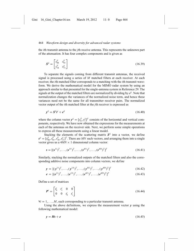
the ith transmit antenna to the jth receive antenna. This represents the unknown partof the attenuation. It has four complex components and is given as
S ij =[
sijhh sij
hv
sijvh sij
vv
](16.39)
To separate the signals coming from different transmit antennas, the receivedsignal is processed using a series of M matched filters at each receiver. At eachreceiver, the ith matched filter corresponds to a matching with the ith transmit wave-form. We derive the mathematical model for the MIMO radar system by using anapproach similar to that presented for the single-antenna system in Reference 29. Thesignals at the output of the matched filters are normalized by dividing by aij. Note thatnormalization changes the variances of the normalized noise term, and hence thesevariances need not be the same for all transmitter–receiver pairs. The normalizedvector output of the ith matched filter at the jth receiver is expressed as
yij = S ijt i + eij (16.40)
where the column vector yij = [yijh , yij
v ]T consists of the horizontal and vertical com-ponents, respectively. We have now obtained the expressions for the measurements ateach of the antennas on the receiver side. Next, we perform some simple operationsto express all these measurements using a linear model.
Stacking the elements of the scattering matrix S ij into a vector, we definesij = [sij
hh, sijhv, sij
vh, sijvv]T . There are MN such vectors, and arranging them into a single
vector gives us a 4MN × 1 dimensional column vector:
s = [(s11)T , . . . , (s1N )T , . . . , (sM1)T , . . . , (sMN)T ]T (16.41)
Similarly, stacking the normalized outputs of the matched filters and also the corre-sponding additive noise components into column vectors, we define
y = [( y11)T , . . . , ( y1N )T , . . . , ( yM1)T , . . . , ( yMN)T ]T (16.42)
e = [(e11)T , . . . , (e1N )T , . . . , (eM1)T , . . . , (eMN)T ]T (16.43)
Define a set of matrices
P i =[
tih ti
v 0 0
0 0 tih ti
v
](16.44)
∀i = 1, . . . , M , each corresponding to a particular transmit antenna.Using the above definitions, we express the measurement vector y using the
following mathematical model:
y = Hs + e (16.45)
Gini 16_Gini_Chapter16.tex March 19, 2012 11: 0 Page 465
Adaptive polarization design for target detection and tracking 465
where
H =
⎡⎢⎢⎢⎢⎢⎢⎢⎢⎢⎢⎢⎣
P1 · · · 0 · · · 0 · · · 0...
. . ....
......
......
0 · · · P1 · · · 0 · · · 0...
......
. . ....
......
0 · · · 0 · · · PM · · · 0...
......
......
. . ....
0 · · · 0 · · · 0 · · · PM
⎤⎥⎥⎥⎥⎥⎥⎥⎥⎥⎥⎥⎦
(16.46)
0 is a zero matrix of dimensions 2 × 4. Terms y and e are 2MN × 1 dimensionalobservation and noise vectors, respectively. Thus, we have reduced our mathematicalmodel to the well-known linear form. We now look at the statistical assumptions madeon these terms.
We assume that the noise terms present in e are uncorrelated and that e followsproper complex Gaussian distribution. A complex random vector ς = ςR + jς I issaid to be proper if Cov(ςR, ςR) = Cov(ς I, ς I) and Cov(ςR, ς I). = −Cov(ς I, ςR).Hence, the covariance matrix of e will be diagonal of the form σ 2I . This diagonalassumption states that the noise components at the outputs of the matched filtersacross the various widely separated receivers over both the polarizations are statisti-cally independent for any given time snapshot. This assumption is reasonable, giventhe wide separation between the antennas [26]. Define this covariance matrix as �e
and assume that it is known. The matrix H is a 2MN × MN dimensional designmatrix whose constituent elements depend on the transmit waveform polarizations.We assume that the vector s, which contains elements from all the scattering matri-ces, is a random vector following proper complex Gaussian distribution with a4MN × 4MN covariance matrix given by �s. We further assume that �s is known.If the random matrices S ij are statistically independent, then �s will have a blockdiagonal structure. However, we do not impose any such structural constraint on �s.Furthermore, we assume that s and e are independent.
16.3.2 Problem formulation
The above mathematical model gives an expression for the observation vector whenthe target is present in the illuminated space. When the target is absent, the observa-tions will consist of only the receiver noise vector e. Hence, the problem of detectingthe target reduces to the following binary hypothesis testing problem:
H0 : y = e (16.47)
H1 : y = Hs + e (16.48)
Therefore, under the null hypothesis, y will have complex Gaussian distribution withzero mean and covariance matrix �e. Under the alternative hypothesis, the inde-pendence of s and e implies that y will follow complex Gaussian distribution withzero mean and covariance matrix given by C +�e, where C = H�sH H denotes thecovariance matrix of Hs. This result in an application of the well-known properties

Gini 16_Gini_Chapter16.tex March 19, 2012 11: 0 Page 466
466 Waveform design and diversity for advanced radar systems
of Gaussian random vectors [31]. Next we describe the Neyman–Pearson detectorfor this problem.
16.3.3 Detector
(1) Test statistic: Under the above-mentioned hypotheses, the probability densityfunctions of the observation vector are given as
f ( y|H0) ∝ 1
|�e|e−yH�−1e y (16.49)
f ( y|H1) ∝ 1
|�e + C|e−yH (�e+C)−1y (16.50)
The Neyman–Pearson lemma states that the likelihood ratio test is the most powerfultest for any given size [32]. The likelihood ratio is given as
f ( y|H0)
f ( y|H1)= |�e + C|
|�e| e−yH (�−1e −(�e+C)−1)y (16.51)
Computing the logarithm of the above expression and ignoring the known constants,we clearly see that yH (�−1
e − (�e + C)−1)y is our test statistic and we compare itwith a threshold before selecting a hypothesis:
yH (�−1e − (�e + C)−1)y ≷H1
H0k (16.52)
where the threshold k is chosen based on the size specified for the test.(2) Estimating covariance matrices: In practice, the covariance matrices needed
for implementing the detector may not be known in advance. In such a scenario, theMLE of these matrices can be substituted to perform the test. Since the observationsfollow Gaussian distribution under both the hypotheses, the MLE of the covariancematrices are given by the corresponding sample covariance matrices [32,33]. Thesample covariance matrices are easy to compute in practice. We assume sufficientnumber of samples to obtain accurate estimates of these covariance matrices. Thevariance of noise at each receiver is calculated before the detector starts functioningby evaluating the sample variance using a large set of training data. The covariancematrix under the alternative hypothesis is estimated by evaluating the sample covari-ance matrix using all the samples of observations in a particular window of timewhen the detector is in use. These two estimated matrices are sufficient for imple-menting the detector. If there is no target in the illuminated space, then these twoestimated matrices will be close to each other, thereby causing the test statistic to fallbelow the threshold.
(3) Performance analysis: To analyse the performance of the above-mentioneddetector, we need to know the distribution of the test statistic under both hypothe-ses. The test statistic is a quadratic form of the complex Gaussian random vector y.It is well known in statistics that a quadratic form zT Uz of a real Gaussian randomvector z with covariance matrix B will follow Chi-square distribution if and only ifthe matrix UB is idempotent [34]. Using this result, we infer that our test statistic doesnot necessarily follow Chi-square distribution for all feasible choices of �e and C

Gini 16_Gini_Chapter16.tex March 19, 2012 11: 0 Page 467
Adaptive polarization design for target detection and tracking 467
because we did not impose any constraint on�s. Hence, it is difficult to find the exactprobability density function (pdf) for it. To study the pdf of our test statistic, we firstbegin with an assumption that C is diagonal. Later, we will extend this approach tothe non-diagonal case by applying proper diagonalization.
Define the lth diagonal element of C as cl and that of �e as vl . Then, the teststatistic reduces to
M∑i=1
N∑j=1
((1
v(2(i−1)N+2j−1)− 1
v(2(i−1)N+2j−1) + c(2(i−1)N+2j−1)
)|yij
h |2)
+M∑
i=1
N∑j=1
((1
v(2(i−1)N+2j)− 1
v(2(i−1)N+2j) + c(2(i−1)N+2j)
)|yij
v |2)
where yijh , yij
v are always independent Gaussian random variables under both hypothe-ses for all transmitter–receiver pairs because of the diagonal assumption of �e
and C . Therefore, the test statistic is a weighted sum of independent Chi-squarerandom variables and it does not necessarily follow the Chi-square distribution. Itsactual distribution depends on the weights. The pdf of a sum of independent randomvariables is obtained by performing multiple convolutions among the constituent pdfs.However, in this case, it is difficult to find the exact solution. Hence, we shall lookfor approximations to the actual pdf.
In Reference 35, the distribution of the weighted sum of Chi-squares is studied.If πq are real positive constants and Nq are independent standard normal random vari-ables ∀q = 1, . . . , K , then the pdf of the Gamma approximation of R = ∑K
q=1 πqN 2q
is given as
fR(r,α,β) = rα−1 e− rβ
βα�(α)(16.53)
where the parameters α and β are given as
α = 1
2
⎛⎜⎝(∑K
q=1 πq
)2
∑Kq=1 π
2q
⎞⎟⎠ (16.54)
β =(
1
2
(∑Kq=1 πq∑Kq=1 π
2q
))−1
(16.55)
� is the gamma function defined as �(α) = ∫∞0 tα−1e−tdt.
Under the null hypothesis, yijh and yij
v have zero mean and variances v(2(i−1)N+2j−1)
and v(2(i−1)N+2j), respectively. Hence, applying the above approximation with appro-priate weights, the parameters of the Gamma distribution are
αH0 =⎛⎜⎝(∑2MN
l=1cl
vl+cl
)2
∑2MNl=1
(cl
vl+cl
)2
⎞⎟⎠ (16.56)
Gini 16_Gini_Chapter16.tex March 19, 2012 11: 0 Page 468
468 Waveform design and diversity for advanced radar systems
βH0 =⎛⎜⎝
∑2MNl=1
cl
vl+cl∑2MNl=1
(cl
vl+cl
)2
⎞⎟⎠
−1
(16.57)
Under the alternative hypothesis, yijh and yij
v have zero mean and vari-ances v(2(i−1)N+2j−1) + c(2(i−1)N+2j−1) and v(2(i−1)N+2j) + c(2(i−1)N+2j), respectively.The parameters of the Gamma approximation are
αH1 =⎛⎜⎝(∑2MN
l=1cl
vl
)2
∑2MNl=1
(cl
vl
)2
⎞⎟⎠ (16.58)
βH1 =⎛⎜⎝
∑2MNl=1
cl
vl∑2MNl=1
(cl
vl
)2
⎞⎟⎠
−1
(16.59)
Note that so far we have assumed a diagonal structure for matrix C in the afore-mentioned discussion. However, we still need to find expressions for the pdf of thetest statistic when C is not diagonal. Diagonalization will be used to extend the anal-ysis even for the case of non-diagonal matrices [36]. Since �e and C are covariancematrices, (�−1
e − (�e + C)−1) will be a Hermitian matrix, which therefore decom-poses into DH�D, where � is a diagonal matrix consisting of eigenvalues as thediagonal elements and D contains the corresponding orthonormal eigenvectors. Thetest statistic now becomes (Dy)H�(Dy). If we show that Dy has a diagonal covariancematrix under both hypotheses, then our analysis extends to the case in which C is notdiagonal also, with appropriate adjustments made to the parameters of the Gammaapproximation. Under H0, Dy is a complex Gaussian random vector with a covariancematrix CovH0 (Dy) = D�eDH , which is diagonal �e = σ 2I and D has orthonormalvectors. Similarly, under H1, Dy is a complex normal random vector with covariancematrix
CovH1 (Dy) = D(�e + C)DH (16.60)
= (D(�e + C)−1DH )−1 (16.61)
= (D((�e + C)−1 −�−1e +�−1
e )DH )−1 (16.62)
= (D�−1e DH −�)−1 (16.63)
which is diagonal. Hence, under both hypotheses, the test statistic is a weightedsum of Chi-square random variables even when matrix C is not diagonal. The onlydifference is that the weights will now be different, and they are defined by thediagonalization process.
After approximating the pdf using the Gamma density, the probability of detec-tion (PD) and the probability of false alarm (PFA) are defined as follows:
PD =∞∫
k
tαH1 −1 e− tβH1
βαH1H1�(αH1 )
dt (16.64)
Gini 16_Gini_Chapter16.tex March 19, 2012 11: 0 Page 469
Adaptive polarization design for target detection and tracking 469
PFA =∞∫
k
tαH0 −1 e− tβH0
βαH0H0�(αH0 )
dt (16.65)
where the parameters αH0 , βH0 , αH1 and βH1 are as mentioned earlier. For a given valueof PFA, the value of the threshold k is calculated easily using the above expressionbecause functions for evaluating the above expressions exist in MATLAB. After find-ing the threshold, PD is calculated accordingly. Note that the value of the thresholdand PD depends on matrix C , which in turn depends on the polarizations of the trans-mitted waveforms. Hence, the performance of the detector is related to the transmitwaveform polarizations.
(4) Optimal design: To find the optimal design, we perform a grid search overthe possible waveform polarizations across all the transmit antennas with the helpof the above expressions for PD and PFA. The optimal design corresponds to thetransmit polarizations that give the maximum PD for a given PFA. Later, we will plotthe receiver operating characteristic (ROC) curves to visualize the improvement inperformance because of the optimal design.
16.3.4 Scalar measurement model
Most of the conventional polarimetric radar systems combine the two received sig-nals linearly and coherently at each receiver to give only a scalar measurement thatdepends on the receive polarization vector. For such systems, the output at eachreceive antenna is modelled as an inner product of the received signal and the receiveantenna polarization [1,29]. This receive polarization vector is optimally chosen alongwith the transmit waveform polarizations in order to achieve improved performance.We now obtain the signal model for such systems. From now on, we refer to thismodel as the scalar measurement model.
Let r j = [r jh, r j
v]T be the polarization vector of the jth receiver, where each of theentries is a complex number. We further assume that ‖r j‖ = 1, ∀j = 1, . . . , N . Therest of the variables remain the same as defined earlier, except that the measurementand the noise at each receiver according to this model will be complex scalars. Thescalar observation at the jth receiver y j(t) is now expressed as follows [15–29]:
y j(t) =M∑
i=1
aijrjT S ijt iwi(t − τ ij) + e j(t) (16.66)
This signal is now passed through a series of matched filters whose outputs areappropriately normalized to move the effect of aij into the noise term. Finally, thenormalized output of the ith matched filter at the jth receiver is given as
yij = rjT S ijt i + eij (16.67)
Stacking all the observations and the noise components into column vectors, in asimilar fashion to the approach used earlier, we obtain MN × 1 dimensional vectorsy and e, respectively. Vector s remains the same as defined earlier. However, matrix H

Gini 16_Gini_Chapter16.tex March 19, 2012 11: 0 Page 470
470 Waveform design and diversity for advanced radar systems
changes and now contains the elements of the receive polarization vectors also. Letus define a set of vectors
ηij =[(
r jhti
h
),(
r jhti
v
),(r j
vtih
),(r j
vtiv
)](16.68)
∀i = 1, . . . , M , each of which corresponds to a particular transmitter–receiver pair.Under this definition, the observation vector is expressed as
y = Hs + e (16.69)
where H is a MN × 4MN dimensional matrix given by
H =
⎡⎢⎢⎢⎢⎢⎢⎢⎢⎢⎢⎢⎣
η11 · · · 0 · · · 0 · · · 0...
. . ....
......
......
0 · · · η1N · · · 0 · · · 0...
......
. . ....
......
0 · · · 0 · · · ηM1 · · · 0...
......
......
. . ....
0 · · · 0 · · · 0 · · · ηMN
⎤⎥⎥⎥⎥⎥⎥⎥⎥⎥⎥⎥⎦
(16.70)
Therefore, we obtain a similar linear model even for the systems with scalar measure-ments. The only difference lies in the dimensionality of some of the vectors in themodel and also the constituent elements of the matrix H . The optimal design for sucha system will not only include optimization over the transmit polarizations t i but willalso include the optimal selection of the receive polarization vectors r j. The problemformulation and analysis of the detector remains the same as for the earlier modelbecause the basic structure of the model is still the same.
16.3.5 Numerical results
We consider a system with two transmit antennas and two receive antennas underthe same target detection scenario as described so far. Hence, there are 16 complexelements in the random vector s. We choose the covariance matrix of this vector tobe of the following form:
�s =
⎡⎢⎢⎣�11
s 0 0 00 �12
s 0 00 0 �21
s 00 0 0 �22
s
⎤⎥⎥⎦ (16.71)
where �ijs represents the covariance matrix of the random vector sij and 0 is a 4 × 4
dimensional zero matrix. Each of these matrices was chosen as follows:
Gini 16_Gini_Chapter16.tex March 19, 2012 11: 0 Page 471
Adaptive polarization design for target detection and tracking 471
�11s =
⎡⎢⎢⎣
0.3 0.1ε 0.1ε 0.1ε0.1ε∗ 0.2 0.1ε 0.1ε0.1ε∗ 0.1ε∗ 0.4 0.1ε0.1ε∗ 0.1ε∗ 0.1ε∗ 0.5
⎤⎥⎥⎦ (16.72)
�12s =
⎡⎢⎢⎣
0.5 0.05ε 0.05ε 0.05ε0.05ε∗ 0.3 0.05ε 0.05ε0.05ε∗ 0.05ε∗ 0.4 0.05ε0.05ε∗ 0.05ε∗ 0.05ε∗ 0.3
⎤⎥⎥⎦ (16.73)
�21s =
⎡⎢⎢⎣
0.4 0.1ε 0.1ε 0.1ε0.1ε∗ 0.3 0.1ε 0.1ε0.1ε∗ 0.1ε∗ 0.2 0.1ε0.1ε∗ 0.1ε∗ 0.1ε∗ 0.4
⎤⎥⎥⎦ (16.74)
�22s =
⎡⎢⎢⎣
0.4 0.05ε 0.05ε 0.05ε0.05ε∗ 0.4 0.05ε 0.05ε0.05ε∗ 0.05ε∗ 0.2 0.05ε0.05ε∗ 0.05ε∗ 0.05ε∗ 0.5
⎤⎥⎥⎦ (16.75)
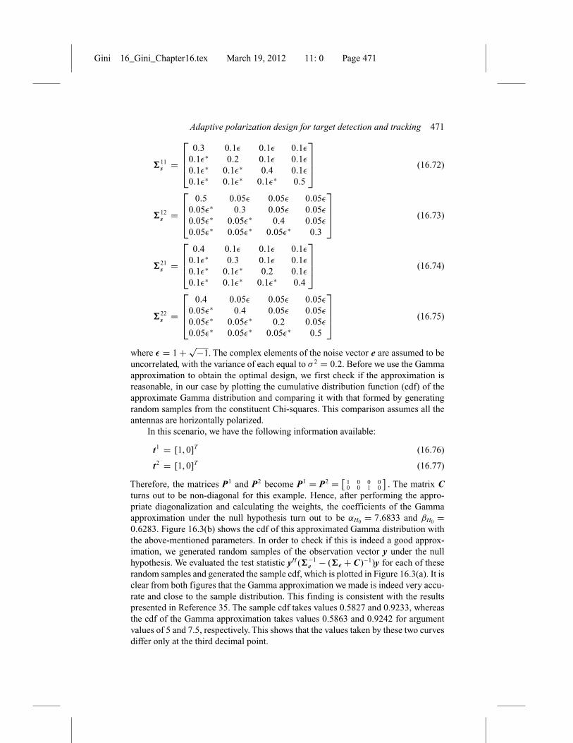
where ε = 1 + √−1. The complex elements of the noise vector e are assumed to beuncorrelated, with the variance of each equal to σ 2 = 0.2. Before we use the Gammaapproximation to obtain the optimal design, we first check if the approximation isreasonable, in our case by plotting the cumulative distribution function (cdf) of theapproximate Gamma distribution and comparing it with that formed by generatingrandom samples from the constituent Chi-squares. This comparison assumes all theantennas are horizontally polarized.
In this scenario, we have the following information available:
t1 = [1, 0]T (16.76)
t2 = [1, 0]T (16.77)
Therefore, the matrices P1 and P2 become P1 = P2 = [1 0 0 00 0 1 0
]. The matrix C
turns out to be non-diagonal for this example. Hence, after performing the appro-priate diagonalization and calculating the weights, the coefficients of the Gammaapproximation under the null hypothesis turn out to be αH0 = 7.6833 and βH0 =0.6283. Figure 16.3(b) shows the cdf of this approximated Gamma distribution withthe above-mentioned parameters. In order to check if this is indeed a good approx-imation, we generated random samples of the observation vector y under the nullhypothesis. We evaluated the test statistic yH (�−1
e − (�e + C)−1)y for each of theserandom samples and generated the sample cdf, which is plotted in Figure 16.3(a). It isclear from both figures that the Gamma approximation we made is indeed very accu-rate and close to the sample distribution. This finding is consistent with the resultspresented in Reference 35. The sample cdf takes values 0.5827 and 0.9233, whereasthe cdf of the Gamma approximation takes values 0.5863 and 0.9242 for argumentvalues of 5 and 7.5, respectively. This shows that the values taken by these two curvesdiffer only at the third decimal point.

Gini 16_Gini_Chapter16.tex March 19, 2012 11: 0 Page 472
472 Waveform design and diversity for advanced radar systems
0 2 4 6 8 100
0.2
0.4
0.6
0.8
1
(a)
f T|H
0(t|H
0)f T
|H0(t|H
0)
0 2 4 6 8 100
0.2
0.4
0.6
0.8
1
(b)
Figure 16.3 Cumulative distribution function of the test statistic for the chosenexample under the null hypothesis: (a) Sample cdf and (b) Gammaapproximation
Now that we have a good enough approximation to the distribution of our teststatistic, we look at how the optimal choice of polarizations improves the performanceof the detector. We fix the complex noise variance to σ 2 = 0.2 and vary the valueof PFA. This method enables us to plot the optimal ROC curve by performing a gridsearch using the analytical results derived earlier. Next, we obtain the reference curvesfor our results by computing the ROC curves assuming that all the transmit antennasare horizontally or vertically polarized. These plots are presented in Figure 16.4, anda significant improvement in performance is clearly visible while using the optimalwaveform polarizations.
So far, we have demonstrated that by optimally selecting the transmit polar-izations, we get performance improvement over conventional MIMO systems withfixed polarizations. Now, we plot the ROC curves for SISO radar with optimal trans-mit polarizations to show the gain in performance because of the multiple widelyseparated antennas. For the SISO system, we consider only the first transmit andreceive antennas in our above-mentioned example. Therefore, the covariance matrixof the scattering vector s becomes �s = �11
s . To make a fair comparison, we trans-mit more power than the power transmitted per antenna while using MIMO radar. Itis clear from Figure 16.5 that 2 × 2 polarimetric MIMO radar system significantlyoutperforms its SISO counterpart even when the SISO system uses four times thetransmit power used by each antenna in the 2 × 2 system.
The complexity of the grid search for optimization using the vector measure-ment model does not increase much with the increase in the number of receivers,because the number of variables over which the optimization is performed dependsonly on the number of transmit antennas. However, with the scalar measurement

Gini 16_Gini_Chapter16.tex March 19, 2012 11: 0 Page 473
Adaptive polarization design for target detection and tracking 473
10–3 10–2 10–1 100
0.65
0.7
0.75
0.8
0.85
0.95
0.9
1
Probability of false alarm (PFA)
Prob
abili
ty o
f det
ectio
n (PD
)
Optimal Transmit PolarizationHorizontal Transmit PolarizationVertical Transmit Polarization
–3
Figure 16.4 ROC curves demonstrating the improvement offered by the optimalchoice of polarizations when σ 2 = 0.2
10–2 10–1 1000.65
0.7
0.75
0.8
0.85
0.95
0.9
Probability of false alarm (PFA)
Prob
abili
ty o
f det
ectio
n (PD
)
1
2x2 PolarimetricMIMO Radar1x1 Polarimetric SISO Radar with 4xTransmit Power/Antenna1x1 Polarimetric SISO Radar with 2xTransmit Power/Antenna
Figure 16.5 ROC curves demonstrating the improvement offered by employingmultiple widely separated antennas compared with single-inputsingle-output systems when σ 2 = 0.2

Gini 16_Gini_Chapter16.tex March 19, 2012 11: 0 Page 474
474 Waveform design and diversity for advanced radar systems
model, the addition of each extra receiver adds extra variables (receive polarizationvectors) in the grid search and makes the calculations more complex. Therefore, inorder to compare the performance of the vector measurement system with that of thescalar measurement system, we use the same numerical example as described so far;however, this time we stick to just two transmitters and one receiver to reduce thecomplexity of the optimization step. The �s matrix now has the following form:
�s =[�11
s 00 �21
s
](16.78)
where matrices �11s and �21
s are chosen to be the same, as defined earlier in thissection. The noise variance remains the same for both the systems because the receivepolarization vectors are assumed to be unit norm. We assume the same noise varianceσ 2 = 0.1 for both systems in order to make a fair comparison. Figure 16.6 comparesthe performance of both systems under the optimal choice of polarization vectors.It clearly shows that by retaining the 2D vector measurements, we get significantlyimproved results as compared with scalar measurement systems. Even though weperform joint optimization over both the transmit and the receive polarizations for thescalar measurement systems, we are still finding just the best linear combination ofthe two received measurements at each receiver. However, combining them linearlyneed not be the overall optimal solution and we might be losing some importantinformation by doing so. This can be avoided by retaining the vector measurements,thereby giving better performance as demonstrated in Figure 16.6.
10–210–3 10–1 100Probability of false alarm (PFA)
Prob
abili
ty o
f det
ectio
n (PD
)
0.55
0.6
0.65
0.7
0.75
0.8
0.85
0.9
0.95
1
Scalar Measurements2D Vector Measurements
Figure 16.6 Comparison of performance between systems with scalarmeasurements and those with 2D vector measurements as a functionof the probability of false alarm when σ 2 = 0.1

Gini 16_Gini_Chapter16.tex March 19, 2012 11: 0 Page 475
Adaptive polarization design for target detection and tracking 475
16.4 Adaptive polarized waveform design for target trackingbased on sequential Bayesian inference
We present a scheme for polarized waveform design for tracking targets in the pres-ence of clutter. This scheme is a combination of sequential Bayesian filtering forparameter estimation and optimal transmitted waveform design in active sensingsystems.
16.4.1 Sequential Bayesian framework for adaptive waveformdesign
This framework for adaptive waveform design includes four phases: (i) creation of adynamic state model and a statistical measurement model, (ii) belief prediction andupdate, (iii) Bayesian state estimation and (iv) optimal waveform selection. They aredescribed in details as follows:
(1) Dynamic state model and measurement model: To formulate a sequentialBayesian estimation, we first consider a state sequence {xk , k ∈ N}, xk ∈ R
nx , whichis assumed to be an unobserved (hidden) Markov process with initial distributionp(x0). The evolution of the state sequence is given by
xk = fk (xk−1, vk−1) (16.79)
where fk : Rnx × R
nv → Rny is a non-linear function of the state; {vk , k ∈ N} is a
process noise sequence and nx and nv are the dimensions of the state and processnoise vectors, respectively. This state model represents our prior knowledge about,e.g. the underlying dynamic movement of a target.
We also have a sequence of measurements {yk , k ∈ N}, yk ∈ Rny . These
measurements are related to the current state vector via the observation equation:
yk = hk (xk , ek ) (16.80)
where hk : Rnx × R
ne → Rny is a non-linear function; {ek , k ∈ R} is a measurement
noise sequence and ny and ne are the dimensions of the measurement and noisevectors, respectively.
(2) Belief prediction and update: We denote by x0:k � {x0, . . . , xk} and y1:k �{y1, . . . , yk}, respectively, the state sequence and the observations up to k . Underthe Bayesian inference framework, all relevant information about x0:k given observa-tions y1:k can be obtained from the posterior probability density (also called belief )p(x0:k |y1:k ). Therefore, our aim is to estimate recursively in time the distributionp(x0:k |y1:k ) and its associated features, including p(xk |y1:k ).
To derive a recursive Bayesian inference process, we consider that the followingconditional independent assumptions for a first-order hidden Markov process aresatisfied.
A1: Conditioned on xk , the current measurements yk are independent of the paststates x0:k−1 and past measurement history y1:k−1, i.e.
p( yk | x0:k , y1:k−1) = p( yk | xk ) (16.81)

Gini 16_Gini_Chapter16.tex March 19, 2012 11: 0 Page 476
476 Waveform design and diversity for advanced radar systems
A2: Conditioned on xk−1, the current state xk is independent of the states x0:k−2 andpast measurement history y1:k−1, i.e.
p(xk | x0:k−1, y1:k−1) = p(xk | xk−1) (16.82)
Based on the above assumptions, we obtain recursive formulas to calculate the newbelief p(x0:k |y1:k ) when the new measurements yk are available, as follows:
p(x0:k | y1:k−1) = p(xk | xk−1)p(x0:k−1 | y1:k−1) (16.83)
and
p(x0:k | y1:k ) = p( yk | xk )p(x0:k | y1:k−1)
p( yk | y1:k−1)(16.84)
where
p( yk | y1:k−1) =∫
p( yk | xk )p(x0:k | y1:k−1)dx0:k (16.85)
For linear and Gaussian state and measurement models, the above equations becomeKalman filters.
Equations (16.83) and (16.84) form a procedure for belief prediction and updatein a recursive belief propagation. In the prediction stage (16.83), we use the proba-bilistic model of the state transition p(xk | xk−1) and the measurement history y1:k−1
to predict the prior pdf of the state at the kth time step. In the update stage (16.84),the current measurement yk (via the likelihood function p(yk | xk )) is used to modifythe prior density p(xk | y1:k−1) to obtain the belief at the current time step.
(3) Bayesian state estimation: At the kth time step, after obtaining the currentbelief p(xk | y1:k ), we can obtain an optimal estimate of the current state xk . In targettracking, this estimate can be used to determine the current target states (e.g. posi-tion and velocity) and environment parameters. Under the Bayesian framework, theestimate is calculated by optimizing a utility function. For example, when we applya minimum-mean-squared error (MMSE) criterion, the estimate is the mean of thebelief p(xk | y1:k ).
(4) Optimal waveform selection: In optimal waveform selection, we use theinformation from the current belief p(xk | y1:k ), together with the state transitiondistribution and measurement model, to optimally select the waveform one step aheadin response to the target state and the environmental situation. Hence, we can achievethe best possible sensing performance.
To derive a mathematical formulation for optimal waveform selection, we firstcreate a utility function according to certain criteria that represent the sensing per-formance; then, we determine the parameters for the next transmitted waveform byoptimizing (e.g. maximizing) this utility function. We denote by J (·) the utility func-tion, θ k+1 the waveform parameters at the (k + 1)th time step, and yk+1(θ k+1) themeasurements at the (k + 1)th time step. At the current time step k , we select the nexttransmitted waveform θ∗
k+1 to be
θ∗k+1 = arg max
θk+1∈J [ p(xk+1 | y1:k , yk+1(θ k+1))] (16.86)

Gini 16_Gini_Chapter16.tex March 19, 2012 11: 0 Page 477
Adaptive polarization design for target detection and tracking 477
where denotes the set of the allowed values for θ k+1 or a library of possiblewaveforms.
We note that the former utility function is related to the belief at the (k + 1)thtime step. To determine this belief, we need the measurements yk+1, which are notavailable at the current time step k . Therefore, we compute the utility function J (·) bymarginalizing out the particular value of yk+1. We observe that for any given yk+1, weobtain a particular value for J (·) acting on the new belief p(xk+1 | y1:k , yk+1(θ k+1)).Now for each waveform parameter θ k+1 we consider the set of all values of J (·) fordifferent values of yk+1. Possibilities for summarizing the set of values of J (·) by asingle quantity include the average, the worst or the best case [37]. For example, ifwe use the average as a utility, the next transmitted waveform is selected by
θ∗k+1 = arg max
θk+1∈Eyk+1|y1:k
{J [ p(xk+1 | y1:k , yk+1(θ k+1))]} (16.87)
where Eyk+1y1:k{·} represents the average over the set of new belief weighted by
p(yk+1|y1:k ).We note that many tracking applications require fast real-time processing. The
trade-off between performance and computation cost should be considered whenchoosing the utility function J (·).
16.4.2 Target dynamic state model and measurement model
We first create a dynamic state model for target tracking. Based on this model, wecan track the target position, velocity and scattering coefficients. We then derive ameasurement model that is the output of the receiver sensor array. This model providesa natural way of incorporating the polarimetric aspects of the target and clutter intothe tracking filter.
(1) Target dynamic state model: In our state model, we include the target scat-tering coefficients that are important, for example, for target identification andclassification [1]. We denote by St the complex scattering matrix representing thepolarization change of the transmit signal upon its reflection on the target:
St =[
shh shv
svh svv
](16.88)
The scattering matrix of the target can be written in terms of the radar polarizationbasis as [38]
St = RTSdR (16.89)
where
● R is a unitary transformation matrix from the target eigenbasis to the radar basis
R =[
cosϑ sin ϑ− sin ϑ cosϑ
]·[
cos ε j sin εj sin ε cos ε
](16.90)
where ϑ is the orientation angle of the target eigenbasis around the line of sightand relative to the radar (−90◦ ≤ ϑ ≤ 90◦), and ε is the ellipticity of the target(−45◦ ≤ ε ≤ 45◦).

Gini 16_Gini_Chapter16.tex March 19, 2012 11: 0 Page 478
478 Waveform design and diversity for advanced radar systems
● Sd is a diagonal matrix representing the target scattering matrix in its eigenpo-larization basis
Sd = me j%
[e j2ν 0
0 tan2 γ e−j2ν
](16.91)
where m is the maximum target amplitude; � is the absolute phase of the scatteringmatrix (−180◦ ≤ � ≤ 180◦); ν is called the skip angle, which is associated withthe depolarization of the reflected signal (−45◦ ≤ ν ≤ 45◦); and γ is called thecharacteristic angle, representing the ability of the target to polarize an incidentunpolarized field (0◦ ≤ γ ≤ 45◦) [1]. These four parameters {m, �, ν, γ } donot change with the target orientation about the line of sight; hence, they arecalled invariant parameters. The decomposition of the scattering matrix for thenon-reciprocal case (i.e. shv �= svh) can be found in Reference 39.Then, we represent the target state at the kth time step as
xk = [ρTk , sT
k ]T (16.92)
where ρk = [xk , yk , zk , xk , yk , zk ]T includes the target position and velocity at the kthtime step in a Cartesian coordinate system, and sk = [ϑk , εk , mk , �k , νk , γk ]T representsthe target scattering parameters.
We assume that (i) the target movement is characterized by a constant velocityand random acceleration, (ii) the target scattering parameters are nearly constantand have random rate of change and (iii) the position and velocity are statisticallyindependent of the scattering coefficients. Then, we obtain a linear target dynamicstate model given by
xk = Fxk−1 + vk−1 =[
Fρ 00 Fs
]xk−1 + vk−1 (16.93)
where
● Fρ is the transition matrix for states ρ as
Fρ =[
I3 TPRII3
0 I3
](16.94)
where In denotes the identity matrix of size n, and TPRI is the pulse repetitioninterval (PRI). Fs = I6 is the transition matrix for state s.
● vk is the independent process noise, representing the uncertainty about the statemodel and is assumed to be zero-mean Gaussian distributed with covariancematrix Q:
Q =[
Qρ 00 Qs
](16.95)

Gini 16_Gini_Chapter16.tex March 19, 2012 11: 0 Page 479
Adaptive polarization design for target detection and tracking 479
where Qρ and Qs denote the covariance matrices for the target acceleration andrate of change of the scattering parameters [40]:
Qρ = qρ
⎡⎢⎢⎢⎢⎢⎢⎣
T 4PRI/4 0 0 T 3
PRI/2 0 00 T 4
PRI/4 0 0 T 3PRI/2 0
0 0 T 4PRI/4 0 0 T 3
PRI/2T 3
PRI/2 0 0 T 2PRI 0 0
0 T 3PRI/2 0 0 T 2
PRI 00 0 T 3
PRI/2 0 0 T 2PRI
⎤⎥⎥⎥⎥⎥⎥⎦
(16.96)
Qs = qsT2PRII6
and qρ and qs are constants.
In this state model, the assumption that the target scattering coefficients varyslowly is suitable for a situation in which the target is far away from the sensor arrayand the target position change during the tracking period is not large compared withthe distance between the target and the sensor array.
In general, the dynamic model for the scattering coefficients is a non-linearfunction with respect to other states; hence, the target dynamic state model will benon-linear. In some cases, it is difficult even to determine a closed-form dynamictransition model for the scattering coefficients. One solution is to assume the statetransition density p(sk+1 | sk ) to be a uniform distribution centred at sk with a radiusequal to the possible maximum value of the change of the scattering coefficientsduring TPRI. That is, we do not provide any prior information about the change of sk
except that sk+1 will be within a certain range.(2) Statistical measurement model: We consider a target characterized by
azimuth φ, elevation ψ , range r, Doppler shift ωD and scattering matrix St . Theseparameters are related to the states x in (16.92). To uniquely identify the polarimetricaspects of a target, polarization diversity is required and the complete EM informa-tion of the signal reflected from the target has to be processed [41]. To provide thesemeasurements, we employ an array of EM vector sensors [11] as the receiver, whereeach sensor measures the six components of the EM field (three electric and threemagnetic components of the received signal).
Consider an array of M vector sensors receiving the signal returns from a target.The complex envelope of the measurements can be expressed as
y(t) = A(φ,ψ)Stξ (t − τ )e jωDt + e(t), t = t1, . . . , tN (16.97)
where
● The matrix A(φ,ψ) = p(φ,ψ) ⊗ V (φ,ψ) is the array response, where ⊗is the Kronecker product; [φ,ψ]T is the bearing angle vector; p(φ,ψ) =[e j2πuTr1/λ, . . . , e j2πuTrM /λ]T represents the phase of the plane wave arriving fromthe direction given by the vector u = [ cosφ cosψ , sin φ cosψ , sinψ]T at the

Gini 16_Gini_Chapter16.tex March 19, 2012 11: 0 Page 480
480 Waveform design and diversity for advanced radar systems
position rm of the mth sensor (m = 1, . . . , M ); λ is the signal wavelength; andV (φ,ψ) is the response of a single vector sensor given by Reference 11:
V (φ,ψ) =
⎡⎢⎢⎢⎢⎢⎢⎣
− sin φ − cosφ sinψcosφ − sin φ sinψ
0 cosψ− cosφ sinψ sin φ− sin φ sinψ − cosφ
cosψ 0
⎤⎥⎥⎥⎥⎥⎥⎦
(16.98)
● The polarized transmit wave ξ (t) is a narrowband signal that can be representedby a complex vector [1,11]:
ξ (t) =[ξh(t)ξv(t)
]= g(t)Q(α)w(β) (16.99)
where
Q(α) =[
cosα sin α− sin α cosα
], w(β) =
[cosβj sin β
](16.100)
Angles α and β are the orientation and ellipticity of the polarization ellipse. Thefunction g(t) represents the scalar complex envelope of the transmitted pulse.The time delay τ = 2r/c, where r is the distance from the target to the sensorarray and c is the wave propagation velocity.
● The vector e(t) is the additive noise corrupting the radar measurements; it repre-sents the thermal noise at the sensors and the reflections from the clutter (targetenvironment).
● N denotes the number of samples during the pulse repetition interval TPRI.
Since ξ (t) is the transmitted signal, the waveform design problem consists of selectingthe envelope g(t) and the polarization angles α and β in (16.99). We denote thesewaveform parameters by θ .
It can be verified that the relationship between the target parameters [φ, ψ , r,ωD, St] and the states x = [ρT , sT ]T is given by
φ = arctan(y
x
)(16.101a)
ψ = arctan
(z√
x2 + y2
)(16.101b)
r = √x2 + y2 + z2 (16.101c)
ωD = 2ωc
c
xx + yy + zz√x2 + y2 + z2
(16.101d)
St = St(s) (16.101e)
where ωc is the carrier frequency, and the relation between St and s is given in(16.89)–(16.91). When we insert (16.101) into the measurement model (16.97), we
Gini 16_Gini_Chapter16.tex March 19, 2012 11: 0 Page 481
Adaptive polarization design for target detection and tracking 481
observe a non-linear relationship between measurements y(t) and state x. We writethis non-linear relationship at the kth time step as
yk (t) = h(t, xk ; θ k ) + ek (t) (16.102)
where
h (t, x; θ ) = A(φ,ψ)Stξ (t − τ )e jωDt , t = t1, . . . , tN (16.103)
When we lump {yk (t), t = t1, . . . , tN } together into a vector, we obtain the followingas measurement model:
yk =⎡⎢⎣
yk (t1)...
yk (tN )
⎤⎥⎦ =
⎡⎢⎣
h(t1, xk ; θ k )...
h(tN , xk ; θ k )
⎤⎥⎦ +
⎡⎢⎣
ek (t1)...
ek (tN )
⎤⎥⎦ (16.104)
= h(xk ; θ k ) + ek .
(3) Polarimetric clutter model: The measurement noise e(t) represents not onlythe thermal noise at the sensors of the receiver but also the reflections from theenvironment surrounding or behind the target. We aim to represent by this model theclutter reflections, for example, in the case for which a target flies above a sea or landsurface.
It is well known that the clutter response is highly dependent on the transmit signalpolarization [1]. We propose a polarimetric clutter model that explicitly accounts forthe polarization of the illuminating signal, and only the clutter scattering coefficientsare represented by a random vector. For estimating the statistical parameters of thisrandom vector, training data recorded with simple two different polarized pulses arerequired [41].
The transmit signal illuminates both the target and the clutter, and their reflec-tions are recorded by the same receiver. Hence, we propose a noise model, similar tomeasurement model (16.97), as
e(t) = A(φ0,ψ0)Scξ (t − τ0) + n(t), t = t1, . . . , tN (16.105)
where n(t) is the additive thermal noise and Sc is the scattering matrix of the clutter.The angles [φ0, ψ0] are the direction in which the radar beam is been steered, whichmight be different from the target angles. The clutter delay τ0 is related to the averageclutter position, and it may also differ from the target delay. For our cases of interest,we consider that the clutter does not introduce Doppler shift; i.e. the clutter veloc-ity can be neglected when compared with the target velocity. The clutter scatteringcoefficients are random variables because they represent the reflections from manyincoherent point scatterers constituting the clutter. Following the model in Refer-ence 41, (16.105) can be rearranged to express the clutter scattering coefficients in avector:
e(t) = A(φ0,ψ0)ξ (t − τ0)Sc + n(t), t = t1, . . . , tN (16.106)

Gini 16_Gini_Chapter16.tex March 19, 2012 11: 0 Page 482
482 Waveform design and diversity for advanced radar systems
where
ξ (t) =[ξh(t) 0 ξv(t)
0 ξv(t) ξh(t)
](16.107)
and
Sc = [schh, sc
vv, schv]T (16.108)
where the variables sc are the scattering coefficients of the clutter.We assume that the thermal noise and the clutter scattering coefficients can be
modelled as
n(t) ∼ CN (0, σ 2I6M), Sc ∼ CN (0,�c) (16.109)
where σ 2 is the noise power, and the clutter covariance matrix can be parameterizedas [41]:
�c =[σ 2
p Q(ϑc)w(εc)w(εc)HQ(ϑc) + σ 2u I2 0
0 px
](16.110)
where σ 2p and σ 2
u are the power of the polarized and unpolarized components of theclutter, ϑc and εc are the orientation and ellipticity angles of the clutter, matrix Q(·)and vector w(·) are defined as in (16.100), and px is the power of the cross-polarizedcomponent of the clutter.
(4) Polarized waveform structure: The design of the polarized waveform involvesselecting the parameters of the signal envelope g(t) and its polarization in (16.99).Here, we consider as an example a linear frequency modulated (LFM) pulse withGaussian envelope, which is defined as
g(t) = (πη2)−1/4 exp[−
(1
2η2− jb
)t2
](16.111)
where η is the pulse length and b is the frequency sweep rate. The signal bandwidthis BW = 7.4ηb [42]. Then, we propose to use the following scheme of polarizedwaveform [43]:
ξ (t) =L−1∑l=0
g(t − lTEPL)Q(αl)w(βl) (16.112)
where L is the number of transmitted LFM pulses and TEPL = 7.4η is theeffective pulse length [42]. Under this scheme, the waveform parameters areθ = [η, b,α0,β0, . . . ,αL−1,βL−1]T .
Note that if the scattering matrix is completely unknown, at least two pulses withdifferent polarization should be transmitted, i.e. L > 0, to uniquely identify St .
16.4.3 Target tracking using sequential Monte Carlo methods
In this section, we develop a target-tracking method based on the proposed dynamicstate model (16.93) and the statistical measurement model (16.104). Since thesemodels are non-linear, we propose a sequential Monte Carlo method (particle filter),
Gini 16_Gini_Chapter16.tex March 19, 2012 11: 0 Page 483
Adaptive polarization design for target detection and tracking 483
which is based on point mass representation of probability densities and is powerfulfor solving non-linear and non-Gaussian Bayesian inference problems.
In contrast to the ordinary sequential Monte Carlo methods, in our proposedapproach, we adopt a Gibbs sampler to draw samples from an importance samplingfunction [44] through which we can handle the potentially large dimension of a statevector. We first describe the ordinary sequential importance sampling (SIS) particlefilter and then we discuss the use of other possible importance sampling functions.
(1) Sequential importance sampling particle filter: The sequential Monte Carlomethod is a technique for implementing a recursive Bayesian filter by Monte Carlosimulations [44]. The key idea is to represent the required posterior density functionby a set of random samples with associated weights and to compute estimates basedon these samples and weights.
Let {x(i)0:k , w(i)
k , i = 1, . . . , Ns} denote a random measure that characterizes thebelief p(x0:k | y1:k ), where {x(i)
0:k , i = 1, . . . , Ns} is a set of support points with asso-ciated weights {w(i)
k , i = 1, . . . , Ns}. Then, the belief at the kth time step can beapproximated as
p(x0:k | y1:k ) ≈Ns∑
i=1
w(i)k δ(x0:k−x(i)
0:k ) (16.113)
where the weights are chosen using the principle of importance sampling [44]. Let{x(i)
0:k , i = 1, . . . , Ns} be samples that are easily generated from a proposal importancedensity function q(x(i)
0:k | y1:k ). Then, the weights in (16.113) are given by Reference 45
w(i)k ∝ p(x(i)
0:k | y1:k )
q(x(i)0:k | y1:k )
(16.114)
For a sequential filtering case where only p(xk | y1:k ) is required at each time step,we can choose the importance density q(·) such that we obtain a weight updateequation [46]:
w(i)k ∝ w(i)
k−1
p( yk | x(i)k )p(x(i)
k | x(i)k−1)
q(x(i)k | x(i)
k−1, yk )(16.115)
and the belief p(xk | y1:k ) can be approximated as
p(xk | y1:k ) ≈Ns∑
i=1
w(i)k δ(xk − x(i)
k ) (16.116)
where {x(i)0:k , i = 1, . . . , Ns} are sampled from the importance density q(xk | x(i)
k−1, yk ).(2) Gibbs sampling–based particle filter: Considering our target tracking prob-
lem, from the dynamic state model (16.93) we observe that if we want to track thetarget position, velocity and scattering coefficients simultaneously, the dimensionof the state space is large. Drawing samples directly from the importance densityq(xk | x(i)
k−1, yk ) is typically inefficient. Hence, we apply a Markov chain Monte Carlo(MCMC) method, a class of iterative simulation-based methods, to sample from the

Gini 16_Gini_Chapter16.tex March 19, 2012 11: 0 Page 484
484 Waveform design and diversity for advanced radar systems
importance density. MCMC methods are a set of procedures that enable the suc-cessful solution of simulation problems for more complex models [47]. The basicidea of MCMC methods is to simulate an ergodic Markov chain whose samples areasymptotically distributed according to a desired density function. In our work, weadopt a classical MCMC algorithm – the Gibbs sampler. Given state θ , the Gibbssampler consists of first defining a partition of the components of θ as θ 1, . . . , θp
(p ≤ dim (θ )), and then sampling successively from the full conditional distributionsp(θ l | θ−l), where θ−l � (θ1, . . . , θ l−1, θ l+1, . . . , θp).
In our developed particle filter, we choose the importance density to be thetransitional prior p(xk | x(i)
k−1), i = 1, . . . , Ns. We adopt the above Gibbs samplingand propose the following method to draw samples from p(xk | x(i)
k−1). Accordingto the state model (16.93), we partition the components of xk as xk = [ρT
k , sTk ]T,
where ρk includes the target position and velocity and sk includes the target scatteringparameters. Then, we derive a Gibbs sampling algorithm to draw samples x(i)
k ∼p(xk | x(i)
k−1) at the kth time step in a particle filter. Such a Gibbs sampling is describedas follows:
● Initialization, j = 0. Set randomly or deterministically:
x(i,0)k =
[(ρ(i,0)
k )T , (s(i,0)k )T
]T
● Iteration j, j = 1, . . . , M , where M is a large number.– Sample ρ(i,j)
k ∼ p(ρk | s(i,j−1)k , x(i)
k−1)– Sample s(i,j)
k ∼ p(sk | ρ(i,j)k , x(i)
k−1)● Installation of ρ(i,M )
k and s(i,M )k into x(i)
k :
x(i)k =
[(ρ(i,M )
k )T , (s(i,M )k )T
]T
Then, the obtained x(i)k is a sample from p(xk | x(i)
k−1).
In a special case where the partitions ρ and s are statistical independent of eachother, the Gibbs sampling can be simplified as
● Sample ρ(i)k ∼ p(ρk | ρ(i)
k−1)● Sample s(i)
k ∼ p(sk | s(i)k−1)
Then, we obtain x(i)k =
[(ρ(i)
k )T , (s(i)k )T
]T
(3) Discussion: In the above proposed Gibbs sampling–based particle filter,we use the simplest importance density function p(xk | x(i)
k−1). However, this impor-tance function does not take into account the current measurements yk , and the statespace is explored without any knowledge of the observations. Therefore, the filtercan be inefficient and it is sensitive to outliers. A natural strategy to overcome thisdisadvantage is to use an optimal importance function that minimizes the variance ofthe importance weights conditional upon the states x(i)
0:k−1 and the measurements y1:k .Such an optimal importance function is given as [46]
q(xk | x(i)k−1, yk ) = p(xk | x(i)
k−1, yk ) (16.117)

Gini 16_Gini_Chapter16.tex March 19, 2012 11: 0 Page 485
Adaptive polarization design for target detection and tracking 485
and the importance weight in (16.115) becomes
w(i)k ∝ w(i)
k−1p( yk | x(i)k−1) (16.118)
However, this optimal importance function suffers from two drawbacks: it requires theability to sample from p(xk | x(i)
k−1, yk ), which is not easy, and it requires the evaluationof p( yk | x(i)
k−1) = ∫ p( yk | xk )p(xk | x(i)k−1)dxk . This integral has no analytical form in
general cases. A practical method to overcome this drawback is to use a Gaussiandensity to approximate the optimal importance function, which allows us to easilydraw samples. The parameters of this Gaussian importance function are evaluatedusing a local linearization of the original optimal importance function [46,48]. Thismethod can be extended to use a sum of Gaussian densities to approximate the optimalimportance function, which can provide a more accurate approximation when theoptimal importance function is multi-modal.
16.4.4 Optimal waveform design based on posterior Cramér–Raobounds
Now, we propose a new optimal waveform design method for target tracking. Thismethod is based on the proposed dynamic state model and the statistical measurementmodel in (16.93) and (16.104), respectively. It is combined with the aforementionedtarget-tracking algorithms and forms an adaptive waveform design scheme.
To pursue the optimization at the kth time step, we develop an algorithm thatpredicts the tracking performance at the (k + 1)th time step when employing specificwaveform parameters. Then, we select the waveform parameters that optimize acertain criterion. Since the target tracking methods are derived under a sequentialBayesian inference framework, we design the waveform selection criterion based ona posterior Cramér–Rao bound (CRB).
(1) Posterior Cramér–Rao bounds: For random parameters, as in our sequentialBayesian filter for target tracking, a lower bound that is analogous to the CRB in anon-random parameter estimation exists and is derived in References 49 and 50. Thislower bound is usually referred to as a posterior CRB (PCRB) or a Bayesian CRB.
We denote by y a vector of measurements and by x a vector of random parame-ters to be estimated. Let p(y, x) be the joint pdf of the pair (y, x), and x = g( y) be anestimate of x. Then, the PCRB on the mean-square estimation error satisfies
� = Ey,x[(g( y) − x)(g( y) − x)T ] ≥ J −1 (16.119)
where J is the Bayesian information matrix (BIM), J −1 is the PCRB, Ey,x[·] denotesexpectation with respect to p(y, x) and the inequality in the equation means that thedifference � − J −1 is a non-negative definite matrix. Let�η
ψ be the m × n matrix ofsecond-order partial derivatives with respect to the m-dimensional parameter ψ andn-dimensional parameter vector η, i.e.
�ηψ =
⎡⎢⎢⎣
∂2
∂ψ1∂η1. . . ∂2
∂ψ1∂ηn...
. . ....
∂2
∂ψm∂η1. . . ∂2
∂ψm∂ηn
⎤⎥⎥⎦ (16.120)
Gini 16_Gini_Chapter16.tex March 19, 2012 11: 0 Page 486
486 Waveform design and diversity for advanced radar systems
Using this notation, the BIM for x is defined as [50]
J = Ey,x[−�ηψ log p(y, x)] (16.121)
From this property, we observe that the PCRB is a lower bound on the error covariancematrix �, and it is related only to the state and measurement models and indepen-dent of the specific estimation methods. Hence, we can use the PCRB as a precisemeasure of the tracking system performance.
(2) Criterion for optimal waveform selection: Consider our target tracking prob-lem: at the kth time step, we want to estimate the state xk using the measurementsy1:k . We denote by X k = [xT
0 , . . . , xTk ]T the sequence of states up to time k . Then, the
BIM of the target states, whose inverse is the PCRB, is defined as
Jk � Ey1:k ,x0:k [−�XkXk
log p( y1:k , x0:k )] (16.122)
This BIM and the corresponding PCRB J −1k are (k + 1)nx × (k + 1)nx matrices. The
lower right nx × nx block of J −1k is the PCRB for estimating xk , and its inverse is the
BIM for estimating xk , denoted by Jk . According to this definition, in our optimalwaveform selection algorithm, at the kth time step we design a criterion based on theBIM Jk+1 to select the waveform to be transmitted at the (k + 1)th time step.
To derive the optimal waveform selection criterion, we adopt the recursive equa-tion in Reference 50 to update BIM Jk+1. For the particular case of a linear state modelwith additive Gaussian noise, this recursive BIM can be written as (see Reference 51)
Jk+1(θ k+1) = [Q + FJk (θ k )−1FT ]−1 + �k+1(θ k+1) (16.123)
where θ k and θ k+1 are the waveform parameters at time step k and k + 1, respectively,the matrices F and Q are defined in (16.93) and (16.95), and
�k+1(θ k+1) = Eyk+1,xk+1 [−�xk+1xk+1
log p( yk+1(θ k+1) | xk+1)] (16.124)
In our sequential waveform design algorithm, we attempt to minimize the erroron the estimation of the target state using the information provided by the state andmeasurement models and the measurement history y1:k . Hence, we modify the matrix�k+1 to include the measurement history and design a criterion based on a new matrix�k+1:
�k+1(θ k+1) = Eyk+1,xk+1|y1:k[−�xk+1
xk+1log p( yk+1(θ k+1) | xk+1)] (16.125)
By replacing �k+1 with �k+1, we use the information from the measurement historyy1:k to improve our prior knowledge on the state xk+1. Mathematically, we replacethe prior density p(xk+1) with p(xk+1 | y1:k ) when calculating �k+1 (see (16.128) fora further understanding). Hence, �k+1 provides more information on state xk+1 than�k+1, and the waveform selection criterion based on �k+1 has the potential to providebetter processing performance. Note that �k+1 is calculated by averaging over all the

Gini 16_Gini_Chapter16.tex March 19, 2012 11: 0 Page 487
Adaptive polarization design for target detection and tracking 487
possible values of yk+1. That means we do not need to know the specific value of thenext measurements to calculate the criterion function. Then, for selecting the optimalparameters of the next transmitted waveform, we propose to use the weighted traceof the inverse of (16.123), replacing �k+1 by �k+1:
θ∗k+1 = arg min
θk+1∈Tr{�J −1
k+1(θ k+1)} (16.126)
where denotes a set of the allowed values for θ k+1 or a library of all possiblewaveforms,� is the weighting matrix used to equalize the magnitude of the differentparameters in the state vector (see also Reference 43), and Jk+1 is defined as in(16.123) replacing �k+1 by �k+1.
(3) Computation of the criterion function: The proposed criterion functiondepends not only on the information provided by the state model F but also onthe measurement model and history, through the term �k+1. To compute the formermatrix, in general, the expectation in (16.125) has no closed-form analytical solutionand must be solved numerically. We propose to use Monte Carlo integration to cal-culate this expectation and merge this numerical procedure into the sequential MonteCarlo method for tracking the target.
To compute the numerical result for �k+1, we define the matrix function
�( yk+1, xk+1) = −�xk+1xk+1
log p( yk+1 | xk+1) (16.127)
Then, we can rewrite �k+1 as
�k+1 =∫
xk+1
⎡⎢⎣ ∫
yk+1
�( yk+1, xk+1)p( yk+1 | xk+1)dyk+1
⎤⎥⎦
× p(xk+1 | y1:k )dxk+1 (16.128)
According to this equation, the expectation to calculate �k+1 can first be takenwith respect to the conditional density function p( yk+1 | xk+1) and then with respectto the density p(xk+1 | y1:k ), i.e.
�k+1 = Exk+1|y1:k[�k+1] (16.129)
�k+1 = Eyk+1|xk+1 [−�xk+1xk+1
log p( yk+1 | xk+1)] (16.130)
Note that �k+1 is the standard Fisher information matrix (FIM) for estimating thestate vector xk+1 based on the observations yk+1.
To calculate (16.129), we need samples of the predicted target state xk+1. We canapply sequential Monte Carlo methods to draw these samples. For a sequential MonteCarlo method, we obtain Ns samples and its associated weights at the kth time stepfrom the belief p(xk | y1:k ) as {x(i)
k , w(i)k ; i = 1, . . . , Ns}. Then, the corresponding
samples and weights of the predicted state are {x(i)k+1, w(i)
k ; i = 1, . . . , Ns}, where
Gini 16_Gini_Chapter16.tex March 19, 2012 11: 0 Page 488
488 Waveform design and diversity for advanced radar systems
x(i)k+1 ∼ p(xk+1 | x(i)
k ). Therefore, the expectation in (16.129) can be computed bythe following two steps:
● For i = 1, . . . , Ns, draw samples x(i)k+1 ∼ p(xk+1 | x(i)
k )● Approximate the matrix �k+1 as
�k+1 ≈Ns∑
i=1
w(i)k �k+1(x(i)
k+1) (16.131)
To calculate (16.130), for each x(i)k+1, we draw Ny identically independently
distributed (i.i.d.) samples {y( j)k+1; j = 1, . . . , Ny} from the likelihood function
p( yk+1 | x(i)k+1). Then, we approximate the FIM �k+1(x(i)
k+1) as
�k+1(x(i)k+1) ≈ 1
Ny
Ny∑j=1
�( y( j)k+1, x(i)
k+1) (16.132)
Therefore, we approximate �k+1 using the Monte Carlo method as
�k+1 ≈ 1
Ny
Ns∑i=1
Ny∑j=1
w(i)k �( y( j)
k+1, x(i)k+1) (16.133)
(4) Computation under Gaussian measurement noise: The Monte Carlo integra-tion for computing �k+1 given by (16.133) is suitable for any statistical measurementmodel. However, if the additive noise ek in the measurement model (16.104) hasGaussian distribution, we can obtain an analytical form for the FIM �k+1; thus, thecost of computing �k+1 using (16.129) can be significantly reduced.
Assuming that the measurement noise ek+1 follows a complex Gaussian distri-bution, the measurement yk+1 given xk+1 is distributed as
yk+1 | xk+1 ∼ CN (h(xk+1),�k+1) (16.134)
where h(·) is defined in (16.104). We also assume that the measurement noise val-ues {ek+1(t), t = t1, . . . , tN } are independent at different sample times. Then, thecovariance matrix in (16.134) can be written as a block diagonal matrix:
�k+1 = diag{�k+1(t1), . . . ,�k+1(tN )} (16.135)
where, if the measurement noise ek+1 follows the model described in section 16.4.2,
�k+1(t) = A(φ0,ψ0)ξ (t − τ0)�cξH(t − τ0)AH(φ0,ψ0) + σ 2I6M (16.136)
Therefore, according to the results in Chapter 15.7 in Reference 20 the FIM in(16.130) is
[�k+1(xk+1)]ij = 2tN∑
t=t1
Re
⎧⎨⎩[∂h(t, xk+1)
∂xk+1,i
]H
�−1k+1(t)
[∂h(t, xk+1)
∂xk+1,j
]⎫⎬⎭ (16.137)
where h(·) is defined in (16.103).
Gini 16_Gini_Chapter16.tex March 19, 2012 11: 0 Page 489
Adaptive polarization design for target detection and tracking 489
(5) Suboptimal criterion function: Computing �k+1 using the Monte Carlo inte-gration is intensive and time demanding because the FIM�k+1 must be evaluated forevery particle. Therefore, we propose a suboptimal criterion function in which thematrix �k+1 is replaced by �k+1 evaluated at the expected predicted state. Therefore,the suboptimal criterion can be computed by the following steps:
● For i = 1, . . . , Ns, draw samples x(i)k+1 ∼ p(xk+1 | x(i)
k )● The expectation of the predicted state is approximated as
xk+1 ≈Ns∑
i=1
w(i)k x(i)
k+1 (16.138)
● Replace �k+1 by �k+1(xk+1) in (16.123).
This suboptimal criterion significatively reduces computation time at the expense ofaccuracy in computing the integral; hence, the selected waveform may not be optimal.
16.4.5 Numerical examples
We use numerical examples to study the performance of the proposed adaptive wave-form design method for tracking targets in the presence of clutter. Through theseexamples, we demonstrate the advantages of the adaptive waveform design schemecompared with the fixed transmitted waveform scheme. First, we provide a descrip-tion of the simulation set-up considered for the target and tracking system, andthen we discuss different numerical examples. The results reported in this sectioncorrespond to the average over 100 Monte Carlo simulations.
Target and clutter. The numerical examples consist of a single target that movesparallel to the horizontal plane at a velocity of 200 m/s. The target trajectory is asection of a circle of radius 1.5 km, which starts at the position r0 = [10, 10] km,as shown in Figure 16.7. We assume that the scattering parameters of the target arepartially known and have the following values: m = 1, ε = 15◦, � = 0◦ν = 0◦ andγ = 20◦; however, its orientation angle ϑ can change as the target moves. In addition,we consider that the clutter covariance parameters have been estimated using trainingdata and that they have the following values: ϑc = 85◦ , εc = 5◦, σ 2
p = 0.4, σ 2u = 0.4
and px = 0.2. The covariance of the clutter will be scaled to fulfil the required target-to-clutter ratio (TCR). We define the TCR following the work by Novak et al. inReference 8:
TCR = ‖[shh, svv, shv]‖2
tr(�c)(16.139)
where shh, svv, shv are the target scattering coefficients defined in (16.88) and ‖ · ‖ isthe norm of the vector.
We define SNR as
SNR = ∫tfti |p(t)|2∂t
∫tfti E[|n(t)|2]∂t
= L
σ 2(tf − ti)(16.140)

Gini 16_Gini_Chapter16.tex March 19, 2012 11: 0 Page 490
490 Waveform design and diversity for advanced radar systems
10 10.1 10.2 10.3 10.4 10.5 10.6 10.7 10.8 10.98.8
9
9.2
9.4
9.6
9.8
10
X Axis (km)
Y A
xis (
km)
True TrajectoryAdaptive WaveformFixed Waveform
Figure 16.7 Comparison of the averaged tracking results between adaptive andfixed waveform schemes
where L is the number of transmitted pulses, σ 2 is the power of the thermal noiseprocess and ti, tf define the time-window during which the system is allowed to trackthe target. p(t) is the pulse envelope of the transmitted signal. For the simulationexamples, these parameters were set up in a way that the system was able to follow atarget in a radial distance between 10 and 25 km.
Transmitted signal. We consider a radar system that transmits one pulse (L = 1)at intervals of TPRI = 250 ms, with a carrier frequency fc = 15 GHz (λ = 20 mm).The maximum signal bandwidth is BWmax = 500 kHz. The system is capable oftransmitting LFM pulses that change length η, frequency rate b and polarizationangles α and β on a pulse-to-pulse basis.
Tracking system. The receiver of the tracker consists of two vector sensors(M = 2) located at r1 = [−0.25λ, 0] and r2 = [0.25λ, 0]. The radar echoes arerecorded at sampling frequency fs = 1 MHz. The system tracks the position andvelocity of the target, as well as its orientation angle; hence, the state vector isx = [x, x, y, y,ϑ]T . The particle filter is implemented using the transitional priorp(xk | x(i)
k−1) as the importance density function to draw Ns = 500 particles. The inten-sity of the process noise is given by qρ = 500 and qs = 50. In addition, we assumethe covariance of the initial state is J −1
0 = diag[500, 500, 200, 200, 0.5]. The weight-ing matrix � is a diagonal matrix whose main diagonal entries are a power of 10intended to equalize the covariance of the different parameters.
Example 1. In this example, we compare the performance of the adaptive and fixedwaveform system assuming that the orientation angle of the target is ϑ = 0◦ along theentire trajectory. For the adaptive system, the wave shape parameters are η = 100 μs
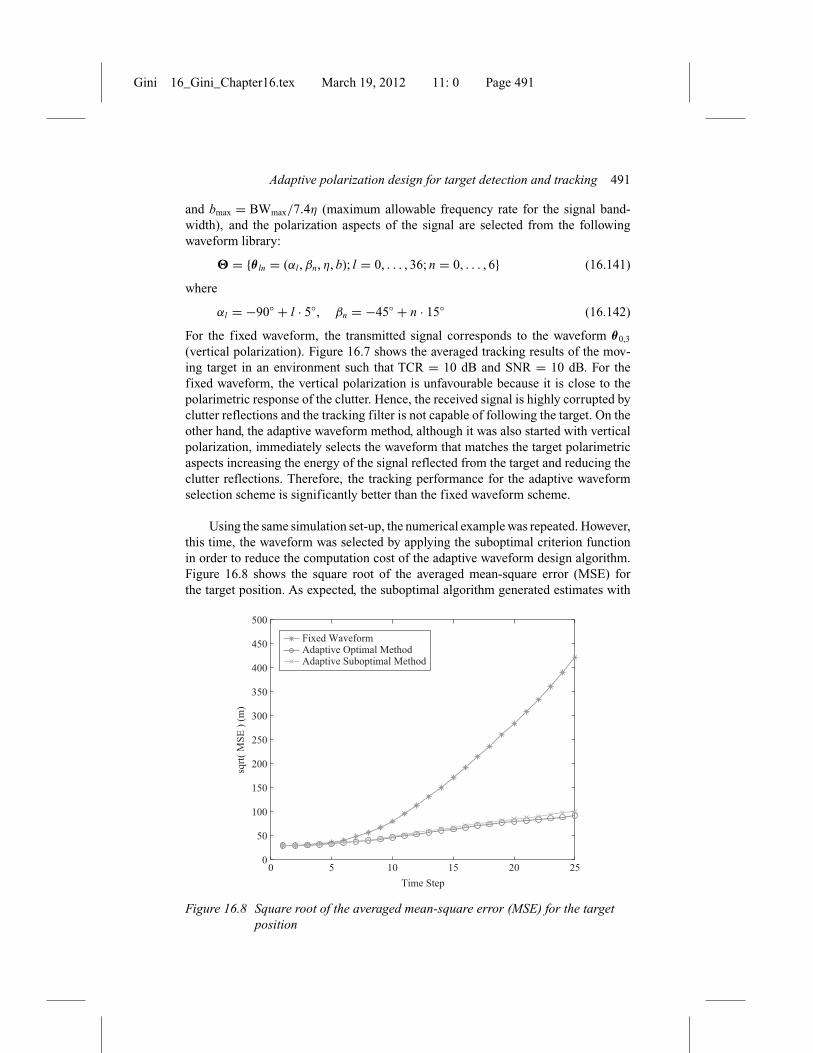
Gini 16_Gini_Chapter16.tex March 19, 2012 11: 0 Page 491
Adaptive polarization design for target detection and tracking 491
and bmax = BWmax/7.4η (maximum allowable frequency rate for the signal band-width), and the polarization aspects of the signal are selected from the followingwaveform library:
= {θ ln = (αl ,βn, η, b); l = 0, . . . , 36; n = 0, . . . , 6} (16.141)
where
αl = −90◦ + l · 5◦, βn = −45◦ + n · 15◦ (16.142)
For the fixed waveform, the transmitted signal corresponds to the waveform θ0,3
(vertical polarization). Figure 16.7 shows the averaged tracking results of the mov-ing target in an environment such that TCR = 10 dB and SNR = 10 dB. For thefixed waveform, the vertical polarization is unfavourable because it is close to thepolarimetric response of the clutter. Hence, the received signal is highly corrupted byclutter reflections and the tracking filter is not capable of following the target. On theother hand, the adaptive waveform method, although it was also started with verticalpolarization, immediately selects the waveform that matches the target polarimetricaspects increasing the energy of the signal reflected from the target and reducing theclutter reflections. Therefore, the tracking performance for the adaptive waveformselection scheme is significantly better than the fixed waveform scheme.
Using the same simulation set-up, the numerical example was repeated. However,this time, the waveform was selected by applying the suboptimal criterion functionin order to reduce the computation cost of the adaptive waveform design algorithm.Figure 16.8 shows the square root of the averaged mean-square error (MSE) forthe target position. As expected, the suboptimal algorithm generated estimates with
0 5 10 15 20 250
50
100
150
200
250
300
350
400
450
500
Time Step
sqrt(
MSE
) (m
)
Fixed WaveformAdaptive Optimal MethodAdaptive Suboptimal Method
Figure 16.8 Square root of the averaged mean-square error (MSE) for the targetposition

Gini 16_Gini_Chapter16.tex March 19, 2012 11: 0 Page 492
492 Waveform design and diversity for advanced radar systems
larger error. However, since the loss of performance is small and the reduction ofcomputation time is significant, we will apply this suboptimal method in the followingexample.
Example 2. We analyse the behaviour of the tracking filter when the state modeldoes not match the target dynamics. In this case, we consider the set-up and waveformlibrary as in the first example; however, the orientation angle of the target ϑ changesfollowing the linear piecewise function depicted in Figure 16.9. The same figureshows the estimated target orientation angle and the waveform polarization angle αselected for transmission by the adaptive algorithm. The same simulation was solvedfor two scenarios: TCR = SNR = 10 dB and TCR = SNR = 15 dB.
In Figure 16.9, it can be observed that the filter tries to track the true orientationangle when it is changing linearly, even though this parameter is defined as constantin the state model. Clearly, the convergence of the estimated orientation angle isfaster when the clutter and noise interference is lower. We note that the filter selectsthe waveform that best matches the estimated target polarization aspects, in order toincrease the energy reflected by the target.
0 5 10 15 20 25
0
2
4
6
8
10
12
14
16
18
20
Time Step
Ang
le (d
egre
e)
True Target OrientationEstimated Target Orientation – Adaptive MethodTransmitted Signal Orientation
Figure 16.9 Averaged orientation angles for two scenarios: TCR = SNR = 10 dB(solid line) and TCR = SNR = 15 dB (dotted line)
16.5 Conclusions
We addressed the problem of designing the optimal signal polarization for target detec-tion and tracking. We reviewed some of our recent results on the adaptive selection

Gini 16_Gini_Chapter16.tex March 19, 2012 11: 0 Page 493
Adaptive polarization design for target detection and tracking 493
of the radar transmit waveform polarizations, where the goal is to explore polariza-tion diversity through an adaptive design. We showed that the optimal selection ofthe polarization significantly improves the detection and tracking performances ofthe radar systems when compared with fixed polarization schemes. We demonstratedthat radar systems supporting agile polarization greatly outperform conventional sens-ing systems. However, to further improve the radar performance, several researchchallenges need to be considered. From the statistical signal processing perspective,these include the development of more realistic models for the target and clutter scat-tering, appropriate performance measures for various critical scenarios and robustbut efficient optimization algorithms. Moreover, the problem of signal polarizationdesign can be extended to other radar applications, such as sequential detection andtarget classification.
Acknowledgements
This work was supported by the Department of Defence under the Air Force Office ofScientific Research MURI Grant FA9550-05-1-0443, ONR Grant N000140810849,and AFOSR Grant FA9550-11-1-0210.
References
[1] D. G. Giuli, ‘Polarimetric modeling and parameters estimation with appli-cations to remote sensing’, Proc. IEEE, vol. 74, pp. 245–269, February1986
[2] W. M. Boerner andY.Yamaguchi, ‘A state-of-the-art review in radar polarime-try and its applications in remote sensing’, IEEE Aerosp. Electron. Syst. Mag.,vol. 5, pp. 3–6, June 1990
[3] G. Sinclair, ‘The transmission and reception of elliptically polarized waves’,Proc. IRE, vol. 38, pp. 148–151, February 1950
[4] E. M. Kennaugh, ‘Effects of type of polarization on echo characteristics’,Technical Report, Antennas Laboratory, The Ohio State University, Columbus,OH, 1954
[5] J. R. Huynen, ‘Phenomenological theory of radar targets’, Ph.D. dissertation,Rotterdam, The Netherlands, 1970
[6] G. Ioannidis and D. Hammers, ‘Optimum antenna polarizations for target dis-crimination in clutter’, IEEE Trans. Antennas Propag., vol. 27, pp. 357–363,May 1979
[7] L. M. Novak, M. B. Sechtin and M. J. Cardullo, ‘Studies of target detectionalgorithms that use polarimetric radar data’, IEEE Trans. Aerosp. Electron.Syst., vol. 25, pp. 150–165, March 1989
[8] R. D. Chaney, M. C. Bud and L. M. Novak, ‘On the performance of polari-metric target detection algorithms’, IEEE Aerosp. Electron. Syst. Mag., vol. 5,pp. 10–15, November 1990

Gini 16_Gini_Chapter16.tex March 19, 2012 11: 0 Page 494
494 Waveform design and diversity for advanced radar systems
[9] R. T. Compton, ‘On the performance of a polarization sensitive adaptivearray’, IEEE Trans. Antennas Propag., vol. 29, pp. 718–725, September1981
[10] E. Ferrara and T. Parks, ‘Direction finding with an array of antennas havingdiverse polarizations’, IEEE Trans. Antennas Propag., vol. 31, pp. 231–236,March 1983
[11] A. Nehorai and E. Paldi, ‘Vector-sensor array processing for electromagneticsource localization’, IEEE Trans. Signal Process., vol. 42, pp. 376–398,February 1994
[12] M. Hurtado and A. Nehorai, ‘Performance analysis of passive low-grazing-angle source localization in maritime environments using vector sensors’,IEEE Trans. Aerosp. Electron. Syst., vol. 43, pp. 780–789, April 2007
[13] S. D. Howard, A. R. Calderbank and W. Moran, ‘A simple signal processingarchitecture for instantaneous radar polarimetry’, IEEE Trans. Inf. Theory,vol. 53, pp. 1282–1289, April 2007
[14] D. A. Garren, A. C. Odom, S. U. Pillai and J. R. Guerci, ‘Full polarizationmatched illumination for target detection and identification’, IEEE Trans.Aerosp. Electron. Syst., vol. 38, pp. 824–837, July 2002
[15] M. Hurtado and A. Nehorai, ‘Polarimetric detection of targets in heavy inho-mogeneous clutter’, IEEE Trans. Signal Process., vol. 56, pp. 1349–1361,April 2008
[16] S. Gogineni and A. Nehorai, ‘Polarimetric MIMO radar with distributed anten-nas for target detection’, IEEE Trans. Signal Process., vol. 58, pp. 1689–1697,March 2010
[17] M. Hurtado, T. Zhao and A. Nehorai, ‘Adaptive polarized waveform design fortarget tracking based on sequential Bayesian inference’, IEEE Trans. SignalProcess., vol. 56, pp. 1120–1133, March 2008
[18] M. Hurtado, J. J. Xiao and A. Nehorai, ‘Target estimation, detection, andtracking: a look at adaptive polarimetric design’, IEEE Signal Process. Mag.,vol. 26, pp. 42–52, January 2009
[19] S. Kay and J. H.Thanos, ‘Optimal transmit signal design for active sonar/radar’,Proc. IEEE Int. Conf Acoust. Spe. Signal Process., vol. 2, pp. 1513–1516,2002
[20] S. M. Kay, Fundamentals of Statistical Signal Processing: Estimation Theory.New Jersey: Prentice-Hall, Inc., 1993
[21] A. D. Maio, G. Alfano and E. Conte, ‘Polarization diversity detection incompound-Gaussian clutter’, IEEE Trans. Aerosp. Electron. Syst., vol. 40,pp. 114–131, January 2004
[22] S. M. Kay, Fundamentals of Statistical Signal Processing: Detection Theory.New Jersey: Prentice-Hall, Inc., 1993
[23] P. Stoica and A. Nehorai, ‘On the concentrated stochastic likelihood functionin array signal processing’, Circ. Syst. Signal Process., vol. 14, pp. 669–674,September 1995
[24] T. W. Anderson, An Introduction to Multivariate Statistical Analysis. Hoboken,NJ: John Wiley & Sons, 2003

Gini 16_Gini_Chapter16.tex March 19, 2012 11: 0 Page 495
Adaptive polarization design for target detection and tracking 495
[25] A. T. James, ‘Distribution of matrix variates and latent roots derived fromnormal samples’, Ann. Math. Stat., vol. 35, pp. 475–501, June 1964
[26] A. M. Haimovich, R. S. Blum and L. J. Cimini, ‘MIMO radar with widelyseparated antennas’, IEEE Signal Process. Mag., vol. 25, pp. 116–129,January 2008
[27] J. Li and P. Stoica, MIMO Radar Signal Processing. Hoboken, NJ: JohnWiley & Sons, 2009
[28] M. Akcakaya and A. Nehorai, ‘MIMO radar sensitivity analysis for targetdetection’, IEEE Trans. Signal Process., vol. 59, pp. 3241–3250, July 2011
[29] J.-J. Xiao and A. Nehorai, ‘Joint transmitter and receiver polarization optimi-zation for scattering estimation in clutter’, IEEE Trans. Signal Process., vol.57, pp. 4142–4147, October 2009
[30] R. Touzi, W. M. Boerner, J. S. Lee and E. Lueneburg, ‘A review of polarime-try in the context of synthetic aperture radar: Concepts and informationextraction’, Can. J. Remote Sensing, vol. 30, no. 3, pp. 380–407, 2004
[31] J. A. Gubner, Probability and Random Processes for Electrical and ComputerEngineers. New York, NY: Cambridge University Press, 2006
[32] L. L. Scharf, Statistical Signal Processing: Detection, Estimation, and TimeSeries Analysis. Reading, MA: Addison-Wesley Publishing Company, Inc.,1991
[33] E. J. Kelly, ‘An adaptive detection algorithm’, IEEE Trans. Aerosp. Electron.Syst., vol. 22, pp. 115–127, March 1986
[34] S. R. Searle, Linear Models. Hoboken, NJ: John Wiley & Sons, 1971[35] A. H. Feiveson and F. C. Delaney, ‘The distribution and properties of a
weighted sum of Chi squares’, NASA Technical Note, May 1968[36] S. M. Kay, Fundamentals of Statistical Signal Processing: Detection Theory.
NJ: Prentice-Hall, Inc., 1998.[37] M. Chu, H. Haussecker and F. Zhao, ‘Scalable information-driven sensor
querying and routing for ad hoc heterogeneous sensor networks’, Int. J.High-Perform. Comput. Appl., vol. 16, pp. 90–110, 2002
[38] J. R. Huynen, ‘Measurement of the target scattering matrix’, Proc. IEEE,vol. 53, pp. 936–946, August 1965
[39] V. Karnychev, V. A. Khlusov, L. P. Ligthart and G. Sharygin, ‘Algorithms forestimating the complete group of polarization invariants of the scattering matrix(sm) based on measuring all sm elements’, IEEE Trans. Geosci. Remote Sens.,vol. 42, pp. 529–539, March 2004
[40] Y. Bar-Shalom, X.-R. Li and T. Kirubarajan, Estimation with Applications toTracking and Navigation. Hoboken, NJ: John Wiley & Sons, 2001
[41] B. Hochwald and A. Nehorai, ‘Polarimetric modeling and parameters estima-tion with applications to remote sensing’, IEEE Trans. Sig. Process., vol. 43,pp. 1923–1935, August 1995
[42] S. P. Sira, A. Papandreou-Suppappola and D. Morrell, ‘Time-varying wave-form selection and configuration for agile sensors in tracking applications’,Proceedings of the IEEE International Conference on Acoustics, Speech, andSignal Processing, vol. 5, Philadelphia, PA, pp. 881–884, March 2005

Gini 16_Gini_Chapter16.tex March 19, 2012 11: 0 Page 496
496 Waveform design and diversity for advanced radar systems
[43] M. Hurtado and A. Nehorai, ‘Optimal polarized waveform design for activetarget parameter estimation using electromagnetic vector sensors’, Proceed-ings of the IEEE International Conference on Acoustics, Speech, and SignalProcessing, vol. 5, Toulousse, France, pp. 1125–1128, May 2006
[44] B. Ristic, S. Arulampalam and N. Gordon, Beyond the Kalman Filter – ParticleFilters for Tracking Applications. Boston, MA: Artech House, 2004
[45] M. S. Arulampalam, S. Maskell, N. J. Gordon and T. Clapp, ‘A tutorial onparticle filters for online nonlinear/non-Gaussian Bayesian tracking’, IEEETrans. Signal Process., vol. 50, pp. 174–178, February 2002
[46] A. Doucet, S. Godsill and C. Andrieu, ‘On sequential Monte Carlo samplingmethods for Bayesian filtering’, Stat. Comput., vol. 10, pp. 197–208, 2000
[47] B. P. Carlin, N. G. Polson and D. S. Stoffer, ‘A Monte Carlo approach tononnormal and nonlinear state-space modeling’, J. Am. Stat. Assoc., vol. 87,June 1992
[48] M. Orton and W. Fitzgerald, ‘A Bayesian approach to tracking multiple targetsusing sensor arrays and particle filters’, IEEE Trans. Signal Process., vol. 5,pp. 216–223, February 2002
[49] H. L. van Trees, Estimation and Modulation Theory. New York, NY: JohnWiley & Sons, 1968
[50] P. Tichavský, C. H. Muravchik and A. Nehorai, ‘Posterior Cramér-Rao boundsfor discrete-time nonlinear filtering’, IEEE Trans. Signal Process., vol. 46,pp. 1386–1396, May 1998
[51] K. L. Bell and H. L. van Tress, ‘Posterior Cramér-Rao bound for trackingtarget bearing’, Proceedings of the 13th Annual Workshop Adaptive SensorArray Processing (ASAP ’05), Lincoln Laboratory, Lexington, MA, June 2005