Adaptive Spatio-Temporal Filters

for

Infrared Target Detection

by

Anusha Muthu Natarajan

Copyright c© Anusha Muthu Natarajan, 2005

A Thesis Submitted to the Faculty of the

Department of Electrical and Computer Engineering

In Partial Fulfillment of the Requirements

For the Degree of

Master of Science

In the Graduate College

The University of Arizona

2 0 0 5

2

3

Statement by Author

This thesis has been submitted in partial fulfillment of requirements for an advanced degree

at The University of Arizona and is deposited in the University Library to be made available to

borrowers under rules of the Library.

Brief quotations from this thesis are allowable without special permission, provided that accu-

rate acknowledgment of source is made. Requests for permission for extended quotation from or

reproduction of this manuscript in whole or in part may be granted by the copyright holder.

Signed:

Approval by Thesis Director

This thesis has been approved on the date shown below:

Dr. Charles M. HigginsDepartment of Electrical and Computer

Engineering

Date

4

acknowledgements

I would like to thank my mom and dad for their unconditional love and support.

I am thankful to Dr. Higgins for his support and guidance throughout my Masters program.

I am thankful to Dr. Barton and Dr. Goodman for serving on my defense committee.

I would also like to thank the Higgins Lab people for making the lab a wonderful place to work.

Lastly, I would like to thank all my friends for being there during hard times.

5

Table of Contents

List of Figures . . . . . . . . . . . . . . . . . . . . . . . . . . . . . . . . . . . . . . . . . . 6

Abstract . . . . . . . . . . . . . . . . . . . . . . . . . . . . . . . . . . . . . . . . . . . . . . 7

Chapter 1. Introduction . . . . . . . . . . . . . . . . . . . . . . . . . . . . . . . . . . . 8

1.1. Organization of the Thesis . . . . . . . . . . . . . . . . . . . . . . . . . . . . . . . . . 9

Chapter 2. Biological Motion Detection Models . . . . . . . . . . . . . . . . . . . 10

2.1. Biological Vision . . . . . . . . . . . . . . . . . . . . . . . . . . . . . . . . . . . . . . 102.2. Motion Models . . . . . . . . . . . . . . . . . . . . . . . . . . . . . . . . . . . . . . . 11

2.2.1. Gradient Type Models . . . . . . . . . . . . . . . . . . . . . . . . . . . . . . . 132.2.2. Correlation Type Models . . . . . . . . . . . . . . . . . . . . . . . . . . . . . 13

2.3. Adelson-Bergen Spatiotemporal Energy Model . . . . . . . . . . . . . . . . . . . . . 142.4. Hassenstein-Reichardt Correlation Motion Model . . . . . . . . . . . . . . . . . . . . 142.5. Response of the Reichardt Detector . . . . . . . . . . . . . . . . . . . . . . . . . . . . 16

Chapter 3. Architecture of the Tracking System . . . . . . . . . . . . . . . . . . . 19

3.1. Global Stabilization Stage . . . . . . . . . . . . . . . . . . . . . . . . . . . . . . . . . 193.2. Target Motion Detection . . . . . . . . . . . . . . . . . . . . . . . . . . . . . . . . . . 213.3. Thresholding . . . . . . . . . . . . . . . . . . . . . . . . . . . . . . . . . . . . . . . . 243.4. Tracking . . . . . . . . . . . . . . . . . . . . . . . . . . . . . . . . . . . . . . . . . . . 25

Chapter 4. Spatio-Temporal Filter Adaptation . . . . . . . . . . . . . . . . . . . . 26

4.1. Adaptation of Filter Temporal Frequency . . . . . . . . . . . . . . . . . . . . . . . . 264.2. Adaptation of Filter Spatial Frequency . . . . . . . . . . . . . . . . . . . . . . . . . . 28

Chapter 5. Characterization Results . . . . . . . . . . . . . . . . . . . . . . . . . . . 30

5.1. Results without Adaptation . . . . . . . . . . . . . . . . . . . . . . . . . . . . . . . . 305.2. Results with Adaptation . . . . . . . . . . . . . . . . . . . . . . . . . . . . . . . . . . 37

Chapter 6. Summary . . . . . . . . . . . . . . . . . . . . . . . . . . . . . . . . . . . . . . 41

Chapter 7. Appendix . . . . . . . . . . . . . . . . . . . . . . . . . . . . . . . . . . . . . . 42

References . . . . . . . . . . . . . . . . . . . . . . . . . . . . . . . . . . . . . . . . . . . . . 43

6

List of Figures

Figure 2.1. Compound eye of the fly . . . . . . . . . . . . . . . . . . . . . . . . . . . . . . 11Figure 2.2. Axonal projection of photoreceptor cells in fly’s eye . . . . . . . . . . . . . . . 12Figure 2.3. Adelson-Bergen Spatio-Temporal Energy model . . . . . . . . . . . . . . . . . 15Figure 2.4. Elaborated Hassenstein-Reichardt Model . . . . . . . . . . . . . . . . . . . . . 17

Figure 3.1. Block diagram of the target detection and tracking system . . . . . . . . . . . 19Figure 3.2. Illustration of background motion stabilization in infrared imagery . . . . . . 20Figure 3.3. Elaborated HR detector, shown with example image outputs at each stage . . 22Figure 3.4. Removal of boundary information from motion output . . . . . . . . . . . . . 24

Figure 4.1. Algorithm for adaptation of filter parameters . . . . . . . . . . . . . . . . . . 27

Figure 5.1. Target selection using spatio-temporal filters . . . . . . . . . . . . . . . . . . . 32Figure 5.2. Effect of sinusoidal background properties on tracking performance of a square

target . . . . . . . . . . . . . . . . . . . . . . . . . . . . . . . . . . . . . . . . . . . . . 34Figure 5.3. Tracking results on real infrared imagery . . . . . . . . . . . . . . . . . . . . . 36Figure 5.4. Adaptation of temporal and spatial frequency using a sinusoidal grating stimulus 38Figure 5.5. Adaptation of temporal and spatial frequency using a square target . . . . . . 40

7

Abstract

We show how nonlinear filters tuned to the spatial and temporal frequency of a moving target may

be used to selectively detect and track certain specified moving objects in an image sequence, while

ignoring other moving objects as well as background movement. Further, we describe an algorithm

for adaptation of the filter parameters to maximize the strength of the filter output as the target

changes in speed or size. We characterize the performance of these tunable filters in detection and

tracking of a moving target in infrared imagery, first for artificially-generated scenes, and then for

real infrared imagery.

Adaptive Spatio-Temporal Filters

for

Infrared Target Detection

Anusha Muthu Natarajan, M.S.The University of Arizona, 2005

Director: Dr. Charles M. Higgins

We show how nonlinear filters tuned to the spatial and temporal frequency of a moving target

may be used to selectively detect and track certain specified moving objects in an image sequence,

while ignoring other moving objects as well as background movement. Further, we describe an

algorithm for adaptation of the filter parameters to maximize the strength of the filter output as the

target changes in speed or size. We characterize the performance of these tunable filters in detection

and tracking of a moving target in infrared imagery, first for artificially-generated scenes, and then

for real infrared imagery.

8

Chapter 1

Introduction

In this thesis, we address the problem of detecting and tracking designated moving ground targets

in infrared imagery collected by a moving airborne imager, in an environment which includes the

possibility of multiple distractor targets. This problem is not generally susceptible to simply tracking

the “hottest” or “coldest” point in the image (Braga-Neto and Goutsias, 1999; Shekerforoush and

Chellappa, 2000), as is often the case in air-to-air interception scenarios (Skolnik, 1962; Blackman

and Popoli, 1999), since background features may be hotter or colder than the target. Rather, it is

necessary to look for coherent target motion in the image while neglecting background motion due

to imager movement relative to the background.

With background motion completely removed, simple frame differencing (Lee et al., 2001; Rosin

and Ellis, 1995; Lipton et al., 1998) would allow the identification of moving objects in the image.

Block-matching algorithms, which are better able to handle background motion, have been used

to compute motion between frames and perform target tracking (Hariharakrishnan et al., 2003;

Zhang and Wu, 2001). Segmentation-based target detection schemes have also been used in this

case (DK et al., 2000; Yilmaz et al., 2003). Yilmaz et al. have presented a method using Gabor filter

responses and global motion compensation to track targets in FLIR imagery (Yilmaz et al., 2001;

Yilmaz et al., 2003). However, these methods provide no way of distinguishing between multiple

targets. To address this problem, we propose the use of spatio-temporal filters (Adelson and Bergen,

1985; Van Santen and Sperling, 1985) to detect visual motion for the purpose of target detection.

Special-purpose hardware systems have been constructed for implementing such filters (Langan,

2004). These filters, originally conceived to model biological visual motion processing, are sensitive

to visual motion in the image over a narrow range of spatial and temporal frequency (STF). Such

filters allow distinction between multiple targets based on direction of motion, speed, and spatial

9

frequency content.

The tunability of these spatio-temporal filters becomes a weakness when the designated target

changes in apparent size or speed, thus altering its STF content. For this reason, we describe an

adaptation algorithm that changes the spatial and temporal frequency tuning of the algorithm as

the interception proceeds to maximize the filter output, and thus keep the filter narrowly tuned to

the target being tracked.

1.1 Organization of the Thesis

In this thesis, we present a target tracking system that utilizes biologically inspired spatiotemporal

filters to track ground targets in infrared imagery. The main focus is on adapting the parameters of

the spatiotemporal filter in order to track targets changing size or speed. The thesis is organized as

follows.

In the second chapter, we present a brief summary of the insect visual system and biological

motion detection models. In the third chapter, we begin by describing the overall tracking system

architecture, including a global motion stabilization stage, a motion detection stage that uses spa-

tiotemporal filters, and thresholding and tracking stages. We explain in detail the algorithms used

for camera motion estimation and elimination, thresholding and tracking. In the fourth chapter, we

describe the adaptation algorithm in detail. In the fifth chapter, we present characterization results

of the tracking system with synthetic and real imagery, and discuss the implications of these results.

The sixth chapter summarizes the work and gives directions for future work. In the appendix, we

present Matlab code of our target detection system.

10

Chapter 2

Biological Motion Detection Models

This chapter briefly discusses various spatiotemporal motion models that have been proposed to

explain the complex visual processing in insects to detect and track objects. Insects are able to

navigate through complex, cluttered environments that are littered with obstacles, and yet do so

with tiny brains and low resolution eyes. The resolution of an insect eye ranges from several hundred

to several thousand pixels which is significantly less than that of most conventional machine vision

systems. Conventional vision systems based on mathematical algorithms tend to become very com-

plicated while biological models of the insect visual system suggest simpler solutions for constrained

tasks like motion detection and target tracking. Insects are a good model system because they

display sophisticated flight control and yet are simple enough that we have been able to deduce a

great deal about the underlying neural circuitry used for such tasks, using physiological techniques.

In the next section, the insect visual system is discussed briefly. The next few sections discuss two

important correlation type spatiotemporal motion models.

2.1 Biological Vision

The visual system of insects (especially the fly) has been widely investigated because of its simplicity

and availability and also because most of the neurons are individually identifiable. The compound

eye of the fly is composed of a large number of facets or ommatidia, each of which faces a slightly

different direction than its neighbors (see Figure 2.1).

When objects in the surroundings of the motionless animal or the animal itself moves, each

contrast edge of the image formed on the retina produces a sequence of excitations in the array of the

photoreceptors (Figure 2.2). The electrical signals produced in the photoreceptor array are processed

11

by neural microcircuits which inform the animal about its motion relative to the surroundings.

The visual systems of vertebrates and anthropods are equipped with directionally-selective motion-

sensitive neurons that produce a strong response to the motion of an object in a particular direction

and produce little or no response to motion in the opposite direction (Franceschini et al., 1989).

Figure 2.1. Compound eye of the fly. The compound eye is comprised of hexagonal facets or ommatidia eachfacing a slightly different direction than the other. Reproduced without permission from www.bath.ac.uk

2.2 Motion Models

Motion information is necessary for depth perception, background separation and other complex

tasks of the visual system. Motion information is computed from the intensity patterns sensed by

the two-dimensional array of photoreceptors. Various models have been proposed which describe

the neural computations underlying motion detection in different ways. However, all local motion

detection models have to satisfy certain minimum requirements (Borst and Egelhaaf, 1989).

• Two inputs: Two inputs are necessary, since motion is a vector that needs two points for its

representation.

12

Figure 2.2. Axonal projection of photoreceptor cells from the retina onto the lamina in the eye of the fly.(a) Optical simulation of two adjacent receptor cells R1 and R6. (b) The axonal projection on the laminais such that R1 and R6 are immediately adjacent (twisted black) photoreceptor cells. (c) The clusteredR1-R6 cells, suggested to increase the signal to noise ratio of the input as received by a movement detector.Reproduced without permission from Franceschini et al. (1989).

13

• Nonlinear interaction: A nonlinear interaction between the input signals is required to

preserve all information about the temporal sequence as a movement detector with linear

interaction cannot be directionally selective.

• Asymmetry: The two channels of a movement detector have to be processed in a slightly

different way in order to discriminate which channel was excited first and which later.

Irrespective of the actual level of description, the various biological motion detection schemes

have been divided into Gradient Type and Correlation type models.

2.2.1 Gradient Type Models

The gradient scheme originated from computer vision and was only later applied to biological vision.

It was proposed to estimate the speed of moving objects from a television signal (Limb and Murphy,

1975; Fennema and Thompson, 1979). In gradient schemes an estimate of local motion is obtained

by relating the simultaneously measured spatial and temporal changes in the local light intensity of

the moving image. This scheme in its mathematically perfect form obtains an exact measurement

of the local velocity by dividing the temporal gradient by the spatial gradient of the pattern (Borst

and Egelhaaf, 1989). Marr and Ullman suggested this scheme as a model for movement detection by

vertebrate cortical cells (Marr and Ullman, 1981). However, Buchner proved that motion detection in

flies is based on correlation-like interactions rather than a gradient computing mechanism (Buchner,

1976).

2.2.2 Correlation Type Models

In correlation schemes motion detection is done by computing a kind of spatiotemporal cross-

correlation of the filtered signals originating from two points in the retinal image. The correlation-

type of movement detector was deduced from behavioral experiments on motion vision in insects

14

(Hassenstein and Reichardt, 1956). The next two sections describe two correlation-type motion

detectors: the Adelson-Bergen Model and the Hassenstein-Reichardt model in detail. Since both

the models are mathematically equivalent, we only present the derivation for the response of the

Reichardt detector in the last section.

2.3 Adelson-Bergen Spatiotemporal Energy Model

Adelson and Bergen suggested that motion can be perceived in continuous or sampled displays, when

there is energy of the appropriate spatiotemporal orientation (Adelson and Bergen, 1985). Hence, a

measure of this spatiotemporal energy can be used to measure the motion in any orientation. This

can be achieved by using spatiotemporally oriented filters. But they are phase sensitive; that is,

their response depends on how the pattern lines up with their receptive field at each moment. By

using two units that act as linear spatiotemporal filters on the input and by squaring and summing

the outputs, a measure of the local motion energy can be extracted. In each sub-unit, there are two

spatial filters followed by two kinds of temporal filters with different delays. The low-pass filtered

responses are combined to get four different responses. Each response is then squared and added to

give the spatiotemporal energy. The two sets of oriented energies are then subtracted to give the

final motion output (see Figure 2.3). The output is independent of position and time and has been

shown to be mathematically equivalent to the response of the Hassenstein-Reichardt detector to be

discussed in the next section.

2.4 Hassenstein-Reichardt Correlation Motion Model

Hassenstein analyzed the optomotor response of the beetle Chlorophanus and inferred that motion

detection by the nervous system requires an interaction of signals from two directly neighboring or

next neighboring ommatidia. This correlation model also accounts for the time-averaged optomotor

response of walking or flying flies to moving patterns (Franceschini et al., 1989).

15

Figure 2.3. Adelson-Bergen Spatio-Temporal Energy model. Sums and differences are used to generatedirectionally selective filters. Sums of squares of quadrature pairs give motion energy for each direction. Thedifference between the rightward and leftward signals gives the final output. Reproduced without permissionfrom Adelson and Bergen (1985)

16

The correlation-type motion detector operates on the retinal light intensity distribution or filtered

versions of it and assumes a multiplication for the interaction of its input channels (Figure 2.4). When

the input to one photoreceptor is appropriately delayed, both the input signals become correlated

resulting in a large motion response. Conversely, when the temporal sequence of the stimulation is

reversed, the separation of both input signals is further increased by detector delay, resulting in only

small motion responses. In order to eliminate input signals that are independent of motion, such

as background luminance, the detector is composed of two mirror-symmetrical subunits. Each of

the subunits consists of a separate delay and multiplication stage. The outputs of the two subunits

are then subtracted leading to responses of the same amplitude but of different signs for motion in

opposite directions (Borst and Egelhaaf, 1989).

2.5 Response of the Reichardt Detector

In this section we present the spatiotemporal motion response of the elaborated Reichardt Detector

to a 2-D sinusoidal grating (see Figure 2.4).

The response of the left spatial filter at (0, 0) is a time waveform of frequency ωt, given by:

S1 =s1

2(1 + C sin(ωtt + φs1)) (2.1)

where C is the contrast of the sinusoidal grating.

The response of the right spatial filter at (x0, y0) is a phase-shifted version of 2.1 is given by:

S2 =s2

2(1 + C sin(ωtt + φs2)) (2.2)

where φs is the spatial phase shift given by ωxx0+ωyy0 in which ωx and ωy are the spatial frequencies

in x and y direction respectively. The spatial filters are meant to introduce quadrature spatial phase

in order to maximize the motion response.

S1 and S2 after high pass filtering are given below:

S1H = Ch1s1 sin(ωtt + φs1 + φ1) (2.3)

17

HPF HPF

LPF LPF

Photoreceptor Photoreceptor

X X

-+ _

Output (O)

S 2H

S 1 S 2

S 2HL

S 1H

S 1HL

SF SF

Figure 2.4. Elaborated Hassenstein-Reichardt Model. The photoreceptor collects visual information whichis then spatial filtered (SF) and high-pass filtered (HPF) to enhance the response to temporal changes in thescene. The HPF stage was a introduced as a modification to the original Hassenstein-Reichardt detector byVan Santen and Sperling (1985). This filtered photoreceptor response and a delayed output from an adjacentphotoreceptor are correlated by a multiplication stage. The difference of two such adjacent correlation stagesgives a direction selective output.

18

S2H = Ch1s2 sin(ωtt + φs2 + φ1) (2.4)

Here, h1 is the magnitude of the frequency response and φ1 is the phase of the frequency response

of the high pass filter.

The delay required by the Reichardt detector is implemented by a low pass filter, so the response

after the delay elements is given by:

S1HL = Ch1h2s1 sin(ωtt + φs1 + φ1 + φ2) (2.5)

S2HL = Ch1h2s2 sin(ωtt + φs2 + φ1 + φ2) (2.6)

Here, h2 is the magnitude of the frequency response and φ2 is the phase of the frequency response

of the low pass filter.

The correlation of these delayed and non-delayed responses is fed to a subtractor to obtain the

final output, which is positive for motion in one direction and negative for motion in the opposite

direction. This final output is given as:

O = S1HL · S2H − S1H · S2HL (2.7)

On further simplification the mean motion repsonse is given by:

< O >= C2h21h2 sin(φ2)s1s2 sin(φs2 − φs1) (2.8)

19

Chapter 3

Architecture of the Tracking System

In this chapter, we explain architecture of the overall tracking system, including a global motion

stabilization stage, motion detection stage that makes use of adaptive spatio-temporal filters, and

an adaptive thresholding and target tracking stage (see Figure 3.1).

3.1 Global Stabilization Stage

In order to make use of visual motion to track the target, it is first necessary to remove the global

background motion due to imager movement relative to the background. With global motion re-

moved, the target will be exposed as a moving object on a static clutter background. If information

about the imager motion is available (perhaps from an onboard inertial guidance system), this infor-

mation could be used to warp the imagery such that global background motion is removed. We here

address the case in which no such ancillary information is available, and thus must be computed

from the image sequence itself.

Global

Image

Stabilization

Raw IR

ImageryStabilized

Imagery

Motion

OutputTarget

Track

Adaptation of filter parametersInformation on platform motion,

if available

Target Detection

by

Visual Motion

Thresholding

Candidate

Targets

Target

Tracking

Figure 3.1. Block diagram of the target detection and tracking system. First is a global image stabilizationstage to remove background motion, followed by a target motion detection stage that uses tuned spatio-temporal filters, a thresholding stage that minimizes the candidates for tracking, and finally a tracking stagethat looks for consistent target motion. Information about the detected target is fed back to optimize thespatiotemporal filter to get a stronger target response.

20

(a) (b)

Figure 3.2. Illustration of background motion stabilization in infrared imagery. (a) In the original imagesequence, upward background motion is seen. (b) In the background-stabilized sequence, the smaller originalframe moves down within the larger frame, while background image features are stabilized.

A variety of sophisticated methods have been used to remove background motion from imagery

(Shekerforoush and Chellappa, 2000; Strehl and Aggarwal, 1999; Basu and Aloimonos, 1990). We

estimate the global translational motion of the image with a simple block matching scheme, by

calculating the mean squared error of the difference between each frame and the previous frame

at a small range of relative two-dimensional displacements. The displacement giving the minimum

mean squared error is chosen as the offset for that frame. We synthesize a background-stabilized

image sequence by placing each original image frame in a larger background-stabilized frame (see

Figure 3.2), at a place that compensates for the pre-computed offsets. Thus the smaller original

frame moves within the larger background-stabilized frame, while background image features are

stabilized in the larger image. This simple process is sufficient to largely remove translational (but

not rotational or expansive) background motion, leaving the target as the primary source of visual

motion. Further, doing this block matching over a small range of possible displacements is less

computationally expensive than many other approaches.

21

3.2 Target Motion Detection

A spatial array of elaborated Hassenstein-Reichardt (HR) motion detectors (Van Santen and Sper-

ling, 1985) is used to perform motion detection in the background-stabilized image sequence. This

motion detector, diagrammed in Figure 3.3, first employs two-dimensional even and odd Gabor

spatial filters (Gabor, 1946) to obtain quadrature spatial phase between the two motion detector

inputs.

s1(x, y) = e(− x2+y2

σ2c

) · cos(ωxc · x + ωyc · y) (3.1)

s2(x, y) = e(−x2+y2

σ2c

) · sin(ωxc · x + ωyc · y) (3.2)

where ωxc and ωyc in the above equations are given by

ωxc = ωsc · cos(θc) (3.3)

ωyc = ωsc · sin(θc) (3.4)

These Gabor filters are tuned to a particular orientation θc, size σc, and center spatial frequency

ωsc. First-order temporal high-pass filters are then used to remove the sustained component of each

image pixel’s response, which does not contribute to the motion computation. First-order temporal

low-pass filters are then used to provide a relative phase delay between two pathways, which is

essential for the motion computation. The time constants τhc and τlc of the high- and low-pass

filters (which in our implementation are the same, τc) set the temporal center frequency of the

tuning (see below). Finally, a multiplicative combination of delayed and un-delayed pathways is

used to compute visual motion. Provided the filter’s spatial and temporal frequency parameters

match the target motion, the target has a positive motion response.

In order to use memory efficiently and improve computation speed, we used a step-by-step

22

HPF

X X

+ _

HPF

LPF LPF

Even

Gabor

Image

Motion Output

Odd

GaborEven gabor filtered image Odd gabor filtered image

High Pass filtered image High Pass filtered image

Low Pass filtered image Low Pass filtered image

Motion image

Global Motion Compensated image

(a) (b)

Figure 3.3. Elaborated HR detector, shown with example image outputs at each stage. (a) Each image inthe sequence is convolved with even and odd Gabor filters, providing quadrature relative spatial phase. High-pass filters remove the sustained component of each pixel’s response, and low-pass filters provide temporalphase delay. The outputs of the high pass filter stages and the low pass filter stages are cross-multipliedand subtracted to get the final motion output. (b) The outputs at each stage of the HR detector are shown.The output of the motion computation clearly indicates the target (in white).

implementation for the low pass filters. The response of the step by step low pass filter is given by

f(n) = (1 − B) · g(n) + B · f(n − 1) (3.5)

Here, B = e(−δtτ

), τ is the time constant of the low pass filter and δt is the discrete time step.

This implementation requires only the preceding low pass filtered output to be stored in memory

instead of storing all the previous inputs like the implementation below.

f(n) = (1 − B)

∞∑

m=0

Bmg(n − m) (3.6)

23

In response to a sinusoidal grating stimulus,

I(x, y, t) = 1/2 · (1 + C · sin(ωx · x + ωy · y + ωt · t)) (3.7)

where C is the contrast, ωx and ωy the spatial frequencies, and ωt the temporal frequency, it can be

shown that the response of the HR motion detector (see Section 2.5) is given by

OHR(ωt, ωx, ωy) =C2

4· (S1S2 sin(φs)) ·

(

H21H2 sin(φ2)

)

(3.8)

S1(ωx, ωy) and S2(ωx, ωy) are respectively the amplitude of the spatial frequency response of the

even and odd Gabor filters. φs is the phase difference between the two inputs to any motion detector,

which are separated in x by a distance ∆x, and in y by a distance ∆y .

φs = ωx · ∆x + ωy · ∆y (3.9)

H1(ωt) and H2(ωt) are respectively the amplitudes of the temporal frequency responses of the high

and low pass filters, and φ2(ωt) is the phase response of the low pass filter. In Equation 3.8, spatial

and temporal frequency response terms have been grouped separately.

The spatial frequency response terms of the detector can be written as

OHR(ωx, ωy) = S1S2 sin(φs) =π2

4σ4

ce(−2π2σ2c (ωx−ωxc)

2+(ωy−ωyc)2) (3.10)

The peak spatial frequency response of the HR detector can be shown to occur approximately at

ωx = ωsc · cos(θc) (3.11)

ωy = ωsc · sin(θc) (3.12)

although at very low spatial frequencies the peak response shifts to a frequency slightly higher than

these due to the sin(φs) term in equation 3.10.

When using first order high-pass and low-pass filters with the same cutoff frequency, the temporal

frequency response of the HR detector can be shown to be

OHR(ωt) =(ωtτc)

3

(1 + (ωtτc)2)2(3.13)

24

(a) (b) (c)

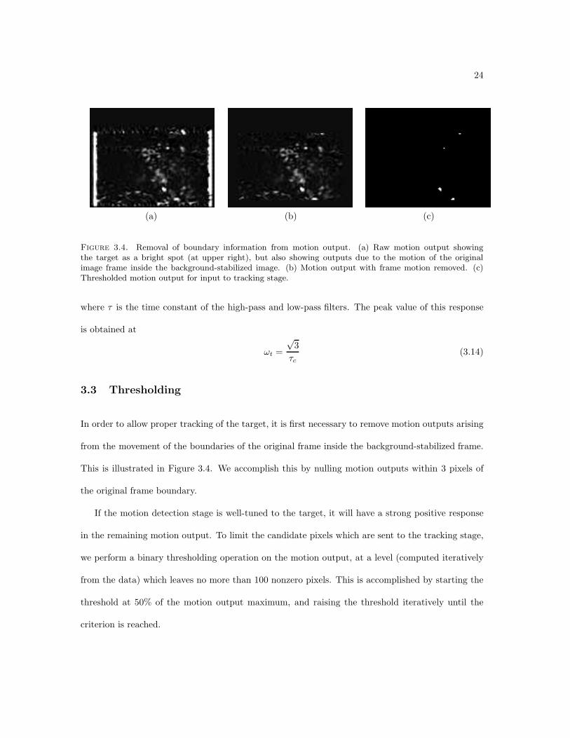
Figure 3.4. Removal of boundary information from motion output. (a) Raw motion output showingthe target as a bright spot (at upper right), but also showing outputs due to the motion of the originalimage frame inside the background-stabilized image. (b) Motion output with frame motion removed. (c)Thresholded motion output for input to tracking stage.

where τ is the time constant of the high-pass and low-pass filters. The peak value of this response

is obtained at

ωt =

√3

τc

(3.14)

3.3 Thresholding

In order to allow proper tracking of the target, it is first necessary to remove motion outputs arising

from the movement of the boundaries of the original frame inside the background-stabilized frame.

This is illustrated in Figure 3.4. We accomplish this by nulling motion outputs within 3 pixels of

the original frame boundary.

If the motion detection stage is well-tuned to the target, it will have a strong positive response

in the remaining motion output. To limit the candidate pixels which are sent to the tracking stage,

we perform a binary thresholding operation on the motion output, at a level (computed iteratively

from the data) which leaves no more than 100 nonzero pixels. This is accomplished by starting the

threshold at 50% of the motion output maximum, and raising the threshold iteratively until the

criterion is reached.

25

3.4 Tracking

Tracking of detected targets is a long-studied topic, and there are many well-known books that

discuss target tracking (Blackman and Popoli, 1999; Blackman, 1986; Bar-Shalom and Li, 1995).

Since tracking as such is not the focus of the present work, we apply a simple tracker to the thresh-

olded motion output. The tracking algorithm observes all potential target pixels in the thresholded

motion output over a sequence of frames. A new potential target track is created for each pixel

which is not within a small radius (5 pixels) of an existing track position. Potential target tracks

are removed when no points have been added to them for 20 frames. The detected target position

is taken from the longest-lived track, indicative of coherent motion over the image sequence. If no

points are added to the longest-lived track in the current frame then the target position from the

previous frame is kept. The track update ratio r is calculated as a fraction of the total number of

frames in which a point is added to the target track. For easy scenarios, this ratio will have a value

close to unity and for difficult scenarios this ratio will have a value close to zero. Hence this ratio is

used as a measure of the tracking performance over an image sequence.

26

Chapter 4

Spatio-Temporal Filter Adaptation

Even if the spatio-temporal filter used for target detection is properly tuned to the target motion at

the beginning of the image sequence, the target might change in apparent size during the sequence

because of a change in distance from the imager, or might change in speed or orientation due to

maneuvering. These changes cause an alteration in the spatial and temporal frequency content of

the target, which will lead to a reduction of the strength of the motion output. In this section, we

describe an algorithm for automatically adapting the spatial and temporal center frequencies of the

HR detector to the target during the image sequence.

The algorithm adapts to changes in the spatial and temporal frequency content of the tar-

get by evaluating the motion output from three spatio-temporal filters instead of one. The three

spatio-temporal filters are chosen from the four filters that result from a combination of two spatial

frequencies (ωsc1, ωsc2) and two temporal frequencies (ωtc1, ωtc2) surrounding the target (see Figure

4.1). The difference in the motion outputs between each pair of filters is used to adapt the spatial

and temporal frequency.

4.1 Adaptation of Filter Temporal Frequency

Adaptation of the filter temporal frequency tuning is equivalent to adaptation of the time constant

of the high-pass and low-pass filters. The algorithm for adaptation of a filter time constant requires

two mostly overlapping temporal filters that result in slight differences in the motion output (Figure

4.1). The two temporal filters are chosen such that the time constant of one of the filters is a fixed

ratio (rt < 1) of the other (thus τc2 = rtτc1). The motion output is evaluated using the spatio-

temporal filter F1 with center frequencies (ωsc1, ωtc1), and F2 with center frequencies (ωsc1, ωtc2)

27

Motion Response

ω s

ωt

Target

F (ωsc1 , ωtc1)1 F (ωsc1 , ωtc2)2

F (ωsc2 , ωtc2)3

Figure 4.1. Algorithm for adaptation of filter parameters. The output of three spatio-temporal filters iscomputed, each offset in spatial or temporal frequency from the target. The difference in response betweenpair F1, F2 is used to modify the temporal frequency, and the pair F2, F3 to modify the spatial frequency.

28

where ωtc1 =√

3/τc1 and ωtc2 =√

3/τc2 (see Equation 3.14). Thus both filters have the same

spatial frequency tuning and differ slightly in temporal frequency tunings. The output of both

spatial-temporal filters is computed, and the time constant is updated as:

τc1 = τc1 + gt · (M1 − M2) (4.1)

τc2 = rt · τc1 (4.2)

where M1 and M2 are respectively the outputs of filters F1 and F2 at the target spatial position

and gt is a temporal adaptation rate parameter. This update is iterated until it stabilizes.

This algorithm serves to move the time constant of both filters such that their response is equal,

and thereby holds the target temporal frequency between the tunings of the two filters as it changes.

For a given set of parameters, it can be shown (by setting the two temporal filters equal) that the

temporal frequency at which the algorithm will stabilize is

ωt,adapt =

√

τc1τc2 +√

τc1τc2(τc1 + τc2)

τc1τc2(4.3)

which is between the center frequencies of the two filters F1 and F2, but not exactly centered

due to asymmetry of the filters.

4.2 Adaptation of Filter Spatial Frequency

Similar to temporal frequency adaptation, the adaptation of the center frequency of the spatial

Gabor filters requires two mostly overlapping spatial filters that result in slight differences in the

motion output. The two spatial filters are chosen such that the center spatial frequency of one is

a ratio (rs < 1) of the other (ωsc2 = rs · ωsc1). The motion output is evaluated using the spatio-

temporal filter F2 with parameters (ωsc1, ωtc2) and F3 with parameters (ωsc2, ωtc2) (Figure 4.1). The

29

output of both spatio-temporal filters is computed and the center spatial frequency is updated as:

ωsc1 = ωsc1 + gs · (M2 − M3) (4.4)

ωsc2 = rs · ωsc1 (4.5)

Again, this algorithm serves to move the center spatial frequency of both filters such that their

response is equal, and thereby holds the target spatial frequency between the tunings of the two

filters as it changes. The adaptation point for the center spatial frequency (ωs,adapt) is the mean of

the center spatial frequencies of the two filters, as the Gabor filters are symmetric:

ωs,adapt =ωsc1 + ωsc2

2(4.6)

30

Chapter 5

Characterization Results

In this chapter, we first demonstrate the performance of the algorithm in selectively tracking targets

based on direction of motion, speed, and spatial frequency content. We then show how properties of

the background like direction of motion relative to target motion, spatio-temporal frequency content

and contrast can affect the target tracking performance, and present sample imagery to illustrate the

performance of the system on real infrared imagery including performance results on the AMCOM

FLIR dataset. Finally, we characterize the performance of the adaptation algorithm using synthetic

targets like sinusoidal gratings and square targets on various backgrounds.

5.1 Results without Adaptation

In this section, the algorithm is evaluated with no adaptation. That is, spatial and temporal fre-

quency parameters are fixed through each experiment.

Using spatio-temporal filters to detect motion gives the advantage to selectively track targets

based on their size, speed and direction of motion. Figure 5.1 shows raw motion outputs for three

scenarios where our system succeeds in making such a distinction. For all three experiments, the

spatial and temporal filters were tuned to track a square target of size 11 by 11 pixels moving at a

speed of 1 pixel/frame to the right (the optimum square target). All targets in our synthetic imagery

are square and have optimum size, speed, direction and contrast unless otherwise stated. In order

to demonstrate size-based selection we used a stimulus having two targets, one of the optimum size

and the other of size 3 by 3 pixels. The strong motion response for the optimum target clearly shows

that the target with the optimum size would be selected for tracking. To demonstrate speed-based

selection we used a stimulus having two targets, one moving at the optimum speed and the other

31

moving at a speed of 2 pixels/frame. The motion output for the optimum target was stronger than

for the other moving at a non-optimum speed and hence would be selected for tracking. To illustrate

selection by orientation, we used a stimulus having two targets, one moving in the preferred direction

and the other moving in the opposite direction. The result showed a strong positive response for the

optimum target and a strong negative response for the other moving in the opposite direction. Since

negative motion responses are ignored (Section 3.3) the optimum target would again be selected for

tracking.

Even when the spatio-temporal filters are well-tuned to the target, the motion response may be

affected by properties of the background. A stimulus consisting of a square target of size 7 by 7 pixels

moving to the right at a speed of 1 pixel/frame superimposed on a moving sinusoidal background

was chosen to characterize the effect of the background on the tracking performance. The numerical

metric M we have used to evaluate tracking performance in each image sequence is

M =r

k + e(5.1)

where r is the track update ratio (Section 3.4), the small constant k (set to 0.01) prevents division

by zero, and e is the RMS error between the actual and predicted target position over the entire

sequence. The above metric will have a higher value if the target track is updated more frequently

and will be reduced if the estimated position of the target is far from the actual position.

In order to study the effect of the orientation of a moving background on tracking performance,

the direction of motion of a sinusoidal background was varied from 0 to 360 degrees. The spatial

and temporal frequencies of the background were tuned to match the spatial-temporal filter and the

background contrast was same as that of the target. Figure 5.2a (solid line) shows the metric plotted

as a percentage of the maximum metric against the direction of motion of the background relative

to the target. The metric has a low value at 0 degrees because there is a strong response from the

background since it is moving in the same direction as the target. The best tracking performance

(M = 0.2867 or 72 percent) was obtained when the background motion was nearly orthogonal to the

32

Stimulus Motion Output

(a)

1 pixel/frame

1 pixel/frame

11 by 11 pixels

3 by 3 pixels

(b)

11 by 11 pixels

11 by 11 pixels

1 pixel/frame

2 pixels/frame

(c)

11 by 11 pixels

11 by 11 pixels

1 pixel/frame

1 pixel/frame

Figure 5.1. Target selection using spatio-temporal filters. The filters were tuned to track a square targetof size 11 by 11 pixels moving at a speed of 1 pixel/frame to the right (the optimum square target). Alltargets are square and have optimum size, speed, contrast and direction unless otherwise stated. (a) Thestimulus presented consisted of two targets, one of the optimum size and the other of size 3 by 3 pixels. Themotion output for the optimum target was 35 times stronger. (b) The stimulus presented had two targets,one moving at the optimum speed and the other moving at double the optimum speed. The motion outputfor the optimum target was 1.76 times stronger. (c) The stimulus presented had two targets, one moving inthe preferred direction and the other moving in the opposite direction. The motion output shows a positiveresponse for the optimum target and a negative response for the other.

33

direction of motion of the target because the target was frequently updated and the estimated target

position was very close to the target for the vast majority of the sequence. The metric around 180

degrees was lower because the target spends significant time superimposed on the bright portions

of the sinusoidal grating, making it invisible. The performance for all angles between 90 and 270

degrees increased when the contrast of the background was reduced to 50 percent (dashed line in

Figure 7a).

To study the effect of background spatial frequency on tracking performance, we next varied the

spatial frequency of the sinusoidal background. The background was moving in the same direction

as the target, its temporal frequency was tuned to match the temporal filter and its contrast was

the same as that of the target. Better performance was obtained when the spatial frequency of

the background did not match the spatial filter tuning (Figure 5.2b). This is because there is less

interference from the background when its spatial frequency does not match that of the spatial filter.

Similar performance was obtained when the temporal frequency of the background was varied.

In our final experiment with background effects, the effect of background contrast on tracking

performance was characterized by varying the contrast of the background from 0 to 100 percent. The

background was moving in the same direction as the target and the spatial and temporal frequencies

of the background were tuned to match the spatial-temporal filter. The metric has a high value

(0.3195 or 81 percent) for contrasts below 25 percent, then falls off steeply to a low value (below 10

percent) and changes only slightly with further increase in contrast (Figure 5.2c). This is because at

any significant contrast the target was visible only when passing the dark portions of the sinusoidal

grating and this caused a significant decrease in tracking performance.

We now present sample images to show the performance of the target detection system on real

imagery collected from an infrared camera on a helicopter at a rate of 30 frames per second. Figure

5.3 shows tracking results for three motion sequences, showing frame 50, 100, 150 and 200 for each.

The target position detected by the tracker matches with the boundary of the target in each of

34

0 45 90 135 180 225 270 315 3600

10

20

30

40

50

60

70

80

90

Direction of motion of the sinusoidal background relative to the target (degrees)

Per

cent

age

of M

etric

to th

e M

axim

um M

etric

0.001 0.01 0.0477 0.1 10

10

20

30

40

50

60

70

80

90

100

Spatial Frequency of the Background (cycles/pixel)

Per

cent

age

of M

etric

to M

axim

um M

etric

Target Spatial Frequency

(a) (b)

0 10 20 30 40 50 60 70 80 90 1000

10

20

30

40

50

60

70

80

90

Contrast of the sinusoidal background

Per

cent

age

of M

etric

to M

axim

um M

etric

(c)

Figure 5.2. Effect of sinusoidal background properties on tracking performance of a square target. Stim-ulus used has a square white target of size 7 by 7 pixels moving to the right at a speed of 1 pixel/framesuperimposed on a moving sinusoidal background. The background has the same contrast as that of thetarget (100 percent), its spatial frequency (0.047 cycles/pixel) and temporal frequency (2.65 Hz) match theoptimum tuning of the spatio-temporal filter, and it moves in the same direction as the target unless other-wise stated. The metric is plotted as a percentage of the maximum metric obtained over all experiments. (a)The direction of motion of the sinusoidal background was varied from 0 to 360 degrees. The solid line showsthe metric for a contrast of 100 percent, and the dashed line shows the percentage metric for a contrast of50 percent. For a background contrast of 100 percent, the best performance (72 percent) was obtained whenthe background motion is nearly orthogonal to the target motion. When the contrast of the background wasreduced to 50 percent, the maximum percentage metric increased to 88 percent. (b) The spatial frequencyof the sinusoidal background was varied from 0.031 to 0.25 cycles/pixel. Best tracking performance wasobtained when the spatial frequency of the background was maximally off-tuned from the target frequency(M = 0.394 or 100 percent). (c) The background contrast was varied from 0 to 100 percent. The maximummetric obtained at a background contrast of 0 percent was 81 percent.

35

the cases. In case (a), the motion sequence has a single target moving towards the left on a desert

background. Over the sequence, the background expands and shifts slightly to the left and right

as the camera follows the target. Gabor filters tuned to the leftward direction were used to track

the target. In case (b), the motion sequence has two targets moving on a highway: one moving up

and to the right and the other opposing it. During the sequence, the background shifts towards the

upper left corner of the image as the camera zooms in on the target. Gabor filters tuned to the

direction of the first target selectively tracked it while ignoring the other target. In case (c), the

motion sequence has a single target moving to the right on a highway surrounded by grasslands.

The background shifts slightly to the right while expanding. Gabor filters tuned to the rightward

direction successfully tracked the target.

Our algorithm also performs well on all appropriate data from the AMCOM FLIR dataset. This

large, well-documented database of air-to-ground FLIR data was provided to the Center for Imag-

ing Science (CIS) at John Hopkins University by the U.S. Army Aviation and Missile Command

(AMCOM). Yilmaz et al. (2003) have presented performance results on the AMCOM dataset in the

form of screenshots, but not using any quantitative metric (Yilmaz et al., 2003). Table 5.1 presents

the RMS error between the actual and predicted target position for three such sequences. It also

shows the metric on the same scale as the previous figures. The first sequence had one target moving

to the left on a highway. The background shifts slightly to the left and right. The second sequence

has one stationary target and one target moving to the left. During the sequence, the background

shifts slightly towards the right and left as the camera zooms in on the moving target. The third

sequence had a target moving to the left on a highway and the background shifts to the right. The

crosshair placed by our tracking algorithm was on the boundary of the target for the vast majority

of the sequence and the non-zero RMS error is only due to a small offset between the true target

position and the estimated target position resulting from the finite size of the target.

36

Frame 50 Frame 100 Frame 150 Frame 200

(a)

(b)

(c)

Figure 5.3. Tracking results on real infrared imagery. Frames 50, 100, 150 and 200 are shown for eachmotion sequence with a white crosshair overlaid at the target position detected by the algorithm. (a) Gaborfilters tuned to the leftward direction were used to track the target moving towards the left in the sequence.(b) The motion sequence has two targets, one moving up and to the right and the other target opposing it.Gabor filters tuned in the direction of the first target selectively tracked it, ignoring the other. (c) Gaborfilters tuned to the rightward direction successfully tracked the target moving to the right.

Sequence RMS Error Metric(%)L1607S 2.0198 86.92L1608S 1.8981 75.37L1720S 3.095 81.28

Table 5.1. Performance on the AMCOM FLIR Dataset

37

5.2 Results with Adaptation

In this section, we present results to characterize the performance of the adaptation algorithm on

synthetic imagery. Adaptation of the spatial and temporal frequency of the filter using a sinusoidal

grating stimulus with no target is illustrated in Figure 5.4. Column 1 shows the adaptation of filter

spatial frequency as the temporal frequency of the stimulus was held constant and its spatial fre-

quency was stepped down and then back up. Column 2 shows the adaptation of temporal frequency

as the spatial frequency of the stimulus was held constant and its temporal frequency was stepped

down and then back up. In both cases, the spatial and temporal frequency of the filter closely

matched that of the changing stimulus after stabilizing. When the spatial filter ratio rs was re-

duced, the algorithm stabilized faster but at the cost of increased oscillations and overshoot (Figure

5.4b1). Increasing the spatial adaptation gain gs resulted in a similar effect. A similar increase in

oscillations and overshoot with the benefit of faster stabilization of temporal frequency was obtained

by increasing the temporal adaptation gain gt (Figure 5.4b2) or reducing the temporal filter ratio

rt. The slight error between the expected value and the actual value of temporal frequency is due

to the finite simulation time step and decreases linearly as the time step is reduced.

Adaptation of filter spatial and temporal frequency to match that of a square target moving on

a black background and on a spatially random background is illustrated in Figure 5.5. A stimulus

having a square target of size 7 by 7 pixels moving at a speed of 1 pixel/frame was presented for

2 seconds and then the size of the target was increased to 9 by 9 pixels for the next 2 seconds. As

expected, the spatial frequency of the filter decreased when the target increased in size (Figure 5.5a).

A stimulus having a square target of size 7 by 7 pixel moving at a speed of 1 pixel/frame was presented

for the first 2 seconds and then its speed was doubled for the next 2 seconds. The temporal frequency

of the filter increased when the speed of the target was increased (Figure 5.5b). The presence of a

spatially random background of contrast 50 percent slightly delayed the stabilization of the algorithm

and also introduced minor oscillations in the adaptation of spatial frequency. Increasing the contrast

38

(1) (2)

(a)0 5 10 15 20 25 30

0.05

0.055

0.06

0.065

0.07

0.075

0.08

0.085

0.09

0.095

0.1

Time (sec)

Filt

er S

patia

l Fre

quen

cy (

cycl

es/p

ixel

)

0 5 10 15 20 25 300.6

0.7

0.8

0.9

1

1.1

1.2

1.3

Time (sec)

Filt

er T

empo

ral F

requ

ency

(H

z)

(b) 0 5 10 15 20 25 300.05

0.055

0.06

0.065

0.07

0.075

0.08

0.085

0.09

0.095

0.1

Time (sec)

Filt

er S

patia

l Fre

quen

cy (

cycl

es/p

ixel

)

0 5 10 15 20 25 300.6

0.7

0.8

0.9

1

1.1

1.2

1.3

1.4

Time(sec)

Filt

er T

empo

ral F

requ

ency

(H

z)

Figure 5.4. Adaptation of temporal and spatial frequency using a sinusoidal grating stimulus. Unlessotherwise stated, the ratio of spatial filter frequencies rs was 0.99, the spatial adaptation gain gs was 0.001,the ratio of temporal filter frequencies rt was 0.9 and the temporal adaptation gain gt was 0.02. Column 1:Adaptation of the spatial frequency of the filter when a sinusoidal stimulus with a spatial frequency of 1/12cycles/pixel was presented for the first 10 seconds, 1/16 cycles/pixel was presented for the next 10 secondsand 1/12 cycles/pixel was presented for the last 10 seconds. The sinusoidal stimulus moves constantly tothe right and has a fixed temporal frequency of 0.5 Hz. The solid line represents the center frequency of thespatial filter and the dotted line signifies the spatial frequency of the sinusoidal stimulus. (a) Parametersare same as given above. (b) rs was reduced to 0.9. Column 2: Adaptation of the temporal frequencyof the filter when a sinusoidal stimulus with a temporal frequency of 1.1 Hz was presented for the first 10seconds, 0.8 Hz was presented for the next 10 seconds and 1.1 Hz was presented for the last 10 seconds. Thesinusoidal stimulus moves constantly to the right and has a fixed spatial frequency of 1/16 cycles/pixel. Thesolid line represents the temporal frequency of the filter and the dotted line signifies the temporal frequencyof the sinusoidal stimulus. (a) Parameters are same as given above. (b) gt was increased to 0.03.

39

of the background to 100 percent further delayed the stabilization of the algorithm.

The spatial frequency at which the algorithm stabilizes corresponds to a peak in the product

of the target spatial frequency spectrum and the spatial frequency response of the spatio-temporal

filter (Figure 5.5c). Similarly, the temporal frequency at which the algorithm stabilizes corresponds

to a local maximum in the product of the target temporal frequency spectrum and the temporal

frequency response of the spatio-temporal filter (Figure 5.5d).

In both cases, the algorithm locks on to one local peak in the product of the target spectrum and

the frequency response of the spatio-temporal filter. The target frequency harmonic to which the

algorithm initially locks can be changed by changing the initial value of the filter spatial frequency

or the time constant of the temporal filter.

40

0 0.5 1 1.5 2 2.5 3 3.5 40.042

0.043

0.044

0.045

0.046

0.047

0.048

Time (sec)

Filt

er S

patia

l Fre

quen

cy (

cycl

es/p

ixel

)

0 0.5 1 1.5 2 2.5 3 3.5 42.6

2.8

3

3.2

3.4

3.6

3.8

4

4.2

4.4

4.6

Time (sec)

Filt

er T

empo

ral F

requ

ency

(H

z)

(a) (b)

0.01 0.02 0.03 0.0426 0.047 0.05 0.06 0.07 0.08 0.09 0

20

40

60

80

100

120

140

Spatial Frequency (cycles/pixel)

Am

plitu

de

0 1 2 2.7 3 4 4.5 5 6 7 8 9 100

0.1

0.2

0.3

0.4

0.5

0.6

0.7

Temporal Frequency (Hz)

Am

plitu

de

(c) (d)

Figure 5.5. Adaptation of temporal and spatial frequency using a square target. (a) A stimulus having awhite square target of size 7 by 7 pixels moving at a constant speed of 1 pixel/ frame on a black backgroundwas presented for the first 2 seconds after which the size of the target was increased to 9 by 9 pixels. Thefilter spatial frequency decreased as expected and stabilized. The dashed line shows the behavior of theadaptation of spatial frequency in the case of a spatially random background with a contrast of 50 percent.(b) A stimulus having a target of size 1 by 1 pixels moving at 1 pixel/frame was presented for the first 2seconds after which the speed was increased to 2 pixels/frame. The filter temporal frequency increased asexpected and stabilized. The dashed line shows the behavior of the adaptation of temporal frequency inthe case of a spatially random background with a contrast of 50 percent. (c) The solid curve indicates theproduct of the one dimensional spatial frequency spectrum of a 7 by 7 pixel target and the spatial frequencyresponse of the spatio-temporal filter (Equation 3.10). The dashed curve indicates a similar plot for the 9 by9 pixel target. The solid and dashed vertical lines indicate the respective spatial frequencies chosen by theadaptation algorithm for the 7 by 7 pixel target and the 9 by 9 pixel target. (d) The solid curve indicatesthe product of the temporal frequency spectrum of a 7 by 7 pixel target moving at 1 pixel/frame and thetemporal frequency response of the spatio-temporal filter (Equation 3.13). The dashed curve indicates asimilar plot for a 7 by 7 pixel target moving at 2 pixels/frame. The solid and dashed vertical lines indicatethe respective temporal frequencies chosen by the adaptation algorithm for a target speed of 1 pixel/frameand 2 pixels/frame.

41

Chapter 6

Summary

In this thesis, we have presented an algorithm to selectively track moving targets in an image

sequence using nonlinear filters tuned to the spatial and temporal frequency of the moving target.

We also presented an algorithm for adaptation of the spatial and temporal frequency of the filter in

order to maximize the strength of the filter output as the target changes in speed or size.

In our results chapter, we presented sample imagery to illustrate the performance of the algorithm

on real infrared imagery obtained from an airborne platform. We also presented performance results

on the AMCOM FLIR dataset. Finally, we presented characterization results of the adaptation

algorithm using synthetic targets like sinusoidal gratings and square targets on various backgrounds.

The results show that our algorithm detects and tracks well even in a highly cluttered environment.

The present version of the algorithm can track a single target moving in a particular direction and

can adapt to changes in size and speed. This algorithm can be extended to track multiple targets

each moving at any direction by using more spatio-temporal filters.

42

Chapter 7

Appendix

43

References

Adelson, E. H. and J. R. Bergen (1985). Spatiotemporal energy models for the perception of motion.

Journal of the Optical Society of America A 2(2): 284–299.

Bar-Shalom, Y. and X.R. Li (1995). Multitarget-Multisensor Tracking: Principles and Techniques.

YBS Publishing, Storrs, CT.

Basu, A. and Y. Aloimonos (1990). A robust, correspondenceless, translation-determining algo-

rithm. International Journal of Robotics Research 9: 35–59.

Blackman, S.S (1986). Multiple Target Tracking with Radar applications. Artech House, Norwood,

MA.

Blackman, S.S. and R.F. Popoli (1999). Design and Analysis of Modern Tracking Systems. Artech

House, Boston, MA.

Borst, A. and M. Egelhaaf (1989). Principles of visual motion detection. tins 12: 297–306.

Braga-Neto, U. and J. Goutsias (1999). Automatic target detection and tracking in forward-

looking infrared image sequences using morphological connected operators. In 33rd Conference of

Information Sciences and Systems, Vol. 3.

Buchner, E. (1976). Elementary movement detectors in an insect visual system. In biolcyb,

pp. 85–101.

DK, Park, Yoon HS, and Won CS (2000). Fast object tracking in digital video. IEEE Transactions

on Consumer Electronics 46(3): 785–790.

Fennema, C.L. and W.B. Thompson (1979). Principles of visual motion detection. Computer

Graphics and Image Processing 9: 301–315.

44

Franceschini, N, N Riehle, and A. Le Nestour (1989). Directionally selective motion detection

by insect neurons. In Stavenga, D. G. and R. C. Hardie, editors, Facets of Vision, pp. 360–390.

Springer, Berlin, Heidelberg.

Gabor, D. (1946). Theory of communication. Journal of the Institute of Electrical Engi-

neers 93: 429–459.

Hariharakrishnan, K., D. Schonfeld, P. Raffy, and F. Yassa (2003). Video tracking using block

matching. In International Conference on Image Processing, 2003, Vol. 3, pp. 945–948.

Hassenstein, B. and W. Reichardt (1956). Systemtheorische analyse der Zeit-, Reihenfolgen- und

Vorzeichenauswertung bei der Bewegungsperzeption des Russelkafers Chlorophanus. Zeitschrift fur

Naturforschung 11b: 513–524.

Langan, J. D. (2004). Computing real-time spatio-temporal motion energy using analog VLSI

image processors. Technical report, Computational Sensors Corporation, Santa Barbara, CA.

http://www.compsensor.com.

Lee, J.S., K.Y. Rhee, and S.D. Kim (2001). Moving target tracking algorithm based on the

confidence measure of motion vectors. In International Conference on Image Processing, 2001,

pp. I: 369–372.

Limb, J.O. and J.A. Murphy (1975). Estimating velocity of moving images in television signals.

CGIP 4(3): 311–327.

Lipton, Alan, Hironobu Fujiyoshi, and Raju Patil (1998). Moving target classification and tracking

from real-time video. In Proc. of the Workshop on Application of Computer Vision, pp. 8 – 14.

IEEE.

Marr, D. and S. Ullman (1981). Directional selectivity and its use in early visual processing.

RoyalP B-211: 151–180.

45

Rosin, P.L. and T. Ellis (1995). Image difference threshold strategies and shadow detection. In

British Machine Vision Conference, 1995, pp. 347–356.

Shekerforoush, H. and R. Chellappa (2000). Multifractal formalism for stabilization, object detec-

tion and tracking in flir sequences. In IEEE International Conference on Image Processing, Vol. 3,

pp. 78–81.

Skolnik, M. I. (1962). Introduction to Radar Systems. McGraw-Hill, New York.

Strehl, A. and J. K. Aggarwal (1999). Detecting moving objects in airborne forward looking infra-

red sequences. In Proc. IEEE Workshop on Computer Vision Beyond the Visible Spectrum (CVPR

1998), Fort Collins, pp. 3–12. IEEE.

Van Santen, J. P. H. and G. Sperling (1985). Elaborated Reichardt detectors. Journal of the Optical

Society of America A 2: 300–320.

Yilmaz, A., K. Shafique, N. Vitoria Lobo, X. Li, T. Olson, and M. A. Shah (2001). Target-tracking

in FLIR imagery using mean-shift and global motion compensation. In CVBVS01, pp. 54–58.

Yilmaz, A., K. Shafique, and M. Shah (2003). Target tracking in airborne forward looking infrared

imagery. Image and Vision Computing 21(7): 623–635.

Zhang, Jason Z. and Q. M. Jonathan Wu (2001). A pyramid approach to motion tracking. Real-

Time Imaging 7(6): 529–544.