chapter 1 the hpf procedure - support.sas.comsupport.sas.com/publishing/pubcat/chaps/59043.pdf ·...
TRANSCRIPT
Chapter 1The HPF Procedure
Chapter Contents
OVERVIEW . . . . . . . . . . . . . . . . . . . . . . . . . . . . . . . . . . . 5
GETTING STARTED . . . . . . . . . . . . . . . . . . . . . . . . . . . . . . 6
SYNTAX . . . . . . . . . . . . . . . . . . . . . . . . . . . . . . . . . . . . . 9Functional Summary. . . . . . . . . . . . . . . . . . . . . . . . . . . . . . 9PROC HPF Statement. . . . . . . . . . . . . . . . . . . . . . . . . . . . .11BY Statement . . . . . . . . . . . . . . . . . . . . . . . . . . . . . . . . .14FORECAST Statement. . . . . . . . . . . . . . . . . . . . . . . . . . . .14ID Statement. . . . . . . . . . . . . . . . . . . . . . . . . . . . . . . . . .19IDM Statement . . . . . . . . . . . . . . . . . . . . . . . . . . . . . . . .22Smoothing Model Specification Options for IDM Statement. . . . . . . . . 24Smoothing Model Parameter Specification Options. . . . . . . . . . . . . . 27Smoothing Model Forecast Bounds Options. . . . . . . . . . . . . . . . . 27
DETAILS . . . . . . . . . . . . . . . . . . . . . . . . . . . . . . . . . . . . .28Accumulation . . . . . . . . . . . . . . . . . . . . . . . . . . . . . . . . .28Missing Value Interpretation . . . . . . . . . . . . . . . . . . . . . . . . . 30Diagnostic Tests. . . . . . . . . . . . . . . . . . . . . . . . . . . . . . . .30Model Selection. . . . . . . . . . . . . . . . . . . . . . . . . . . . . . . .30Transformations. . . . . . . . . . . . . . . . . . . . . . . . . . . . . . . .31Parameter Estimation. . . . . . . . . . . . . . . . . . . . . . . . . . . . .31Missing Value Modeling Issues. . . . . . . . . . . . . . . . . . . . . . . . 31Forecasting. . . . . . . . . . . . . . . . . . . . . . . . . . . . . . . . . . .31Inverse Transformations. . . . . . . . . . . . . . . . . . . . . . . . . . . .31Statistics of Fit. . . . . . . . . . . . . . . . . . . . . . . . . . . . . . . . .32Forecast Summation. . . . . . . . . . . . . . . . . . . . . . . . . . . . . .32Comparison to the Time Series Forecasting System. . . . . . . . . . . . . 32Data Set Output. . . . . . . . . . . . . . . . . . . . . . . . . . . . . . . .32OUT= Data Set . . . . . . . . . . . . . . . . . . . . . . . . . . . . . . . .32OUTEST= Data Set. . . . . . . . . . . . . . . . . . . . . . . . . . . . . .33OUTFOR= Data Set. . . . . . . . . . . . . . . . . . . . . . . . . . . . . .33OUTSTAT= Data Set . . . . . . . . . . . . . . . . . . . . . . . . . . . . .34OUTSUM= Data Set . . . . . . . . . . . . . . . . . . . . . . . . . . . . .35OUTSEASON= Data Set. . . . . . . . . . . . . . . . . . . . . . . . . . .36OUTTREND= Data Set. . . . . . . . . . . . . . . . . . . . . . . . . . . .37Printed Output. . . . . . . . . . . . . . . . . . . . . . . . . . . . . . . . .37

4 � Chapter 1. The HPF Procedure
ODS Table Names. . . . . . . . . . . . . . . . . . . . . . . . . . . . . . .39ODS Graphics (Experimental). . . . . . . . . . . . . . . . . . . . . . . . . 39
EXAMPLES . . . . . . . . . . . . . . . . . . . . . . . . . . . . . . . . . . .42Example 1.1. Automatic Forecasting of Time Series Data. . . . . . . . . . 42Example 1.2. Automatic Forecasting of Transactional Data. . . . . . . . . 44Example 1.3. Specifying the Forecasting Model. . . . . . . . . . . . . . . 45Example 1.4. Extending the Independent Variables for Multivariate Forecasts46Example 1.5. Forecasting Intermittent Time Series Data. . . . . . . . . . . 47Example 1.6. Illustration of ODS Graphics (Experimental). . . . . . . . . 49
REFERENCES . . . . . . . . . . . . . . . . . . . . . . . . . . . . . . . . . .52

Chapter 1The HPF ProcedureOverview
The HPF (High-Performance Forecasting) procedure provides a quick and automaticway to generate forecasts for many time series or transactional data in one step. Theprocedure can forecast millions of series at a time, with the series organized intoseparate variables or across BY groups.
• For typical time series, you can use the following smoothing models:
– Simple– Double– Linear– Damped Trend– Seasonal– Winters Method (additive and multiplicative)
• Additionally, transformed versions of these models are provided:
– Log– Square Root– Logistic– Box-Cox
• For intermittent time series (series where a large number of values are zero-valued), you can use an intermittent demand model such as Croston’s Methodand Average Demand Model.
Experimental graphics are now available with the HPF procedure. For more informa-tion, see the“ODS Graphics”section on page 39.
All parameters associated with the forecast model are optimized based on the data.Optionally, the HPF procedure can select the appropriate smoothing model for youusing holdout sample analysis based on one of several model selection criteria.
The HPF procedure writes the time series extrapolated by the forecasts, the seriessummary statistics, the forecasts and confidence limits, the parameter estimates, andthe fit statistics to output data sets. The HPF procedure optionally produces printedoutput for these results utilizing the Output Delivery System (ODS).
The HPF procedure can forecast both time series data, whose observations are equallyspaced by a specific time interval (e.g., monthly, weekly), or transactional data, whoseobservations are not spaced with respect to any particular time interval. Internet, in-ventory, sales, and similar data are typical examples of transactional data. For trans-actional data, the data is accumulated based on a specified time interval to form a
6 � Chapter 1. The HPF Procedure
time series. The HPF procedure can also perform trend and seasonal analysis ontransactional data.
Additionally, the Time Series Forecasting System of SAS/ETS software can be usedto interactively develop forecasting models, estimate the model parameters, evaluatethe models’ ability to forecast, and display these results graphically. Refer to Chapter33, “Overview of the Time Series Forecasting System,” (SAS/ETS User’s Guide) fordetails.
Also, the EXPAND procedure can be used for the frequency conversion and transfor-mations of time series. Refer to Chapter 16, “The EXPAND Procedure,” (SAS/ETSUser’s Guide) for details.
Getting Started
The HPF procedure is simple to use for someone who is new to forecasting, and yetat the same time it is powerful for the experienced professional forecaster who needsto generate a large number of forecasts automatically. It can provide results in outputdata sets or in other output formats using the Output Delivery System (ODS). Thefollowing examples are more fully illustrated in the“Examples”section on page 42.
Given an input data set that contains numerous time series variables recorded at a spe-cific frequency, the HPF procedure can automatically forecast the series as follows:
PROC HPF DATA=<input-data-set> OUT=<output-data-set>;ID <time-ID-variable> INTERVAL=<frequency>;FORECAST <time-series-variables>;RUN;
For example, suppose that the input data setSALES contains numerous sales datarecorded monthly, the variable that represents time isDATE, and the forecasts are tobe recorded in the output data setNEXTYEAR. The HPF procedure could be used asfollows:
proc hpf data=sales out=nextyear;id date interval=month;forecast _ALL_;
run;
The above statements automatically select the best fitting model, generate forecastsfor every numeric variable in the input data set (SALES) for the next twelve months,and store these forecasts in the output data set (NEXTYEAR). Other output datasets can be specified to store the parameter estimates, forecasts, statistics of fit, andsummary data.
If you want to print the forecasts using the Output Delivery System (ODS), then youneed to add PRINT=FORECASTS:
Getting Started � 7
proc hpf data=sales out=nextyear print=forecasts;id date interval=month;forecast _ALL_;
run;
Other results can be specified to output the parameter estimates, forecasts, statisticsof fit, and summary data using ODS.
The HPF procedure can forecast both time series data, whose observations are equallyspaced by a specific time interval (e.g., monthly, weekly), or transactional data, whoseobservations are not spaced with respect to any particular time interval.
Given an input data set containing transactional variables not recorded at any specificfrequency, the HPF procedure accumulates the data to a specific time interval andforecasts the accumulated series as follows:
PROC HPF DATA=<input-data-set> OUT=<output-data-set>;ID <time-ID-variable> INTERVAL=<frequency>
ACCUMULATE=<accumulation>;FORECAST <time-series-variables>;
RUN;
For example, suppose that the input data setWEBSITES contains three variables(BOATS, CARS, PLANES), that are Internet data recorded on no particular timeinterval, and the variable that represents time is TIME, which records the time of theWeb hit. The forecasts for the total daily values are to be recorded in the output datasetNEXTWEEK. The HPF procedure could be used as follows:
proc hpf data=websites out=nextweek lead=7;id time interval=dtday accumulate=total;forecast boats cars planes;
run;
The above statements accumulate the data into a daily time series and automaticallygenerate forecasts for theBOATS, CARS, andPLANES variables in the input dataset (WEBSITES) for the next seven days and store the forecasts in the output dataset (NEXTWEEK).
The HPF procedure can specify a particular forecast model or select from severalcandidate models based on a selection criterion. The HPF procedure also supportstransformed models and holdout sample analysis.
Using the previousWEBSITES example, suppose that you want to forecast theBOATS variable using the best seasonal forecasting model that minimizes the meanabsolute percent error (MAPE), theCARS variable using the best nonseasonal fore-casting model that minimizes the mean square error (MSE) using holdout sampleanalysis on the last five days, and thePLANES variable using the Log WintersMethod (additive). The HPF procedure could be used as follows:

8 � Chapter 1. The HPF Procedure
proc hpf data=websites out=nextweek lead=7;id time interval=dtday accumulate=total;forecast boats / model=bests select=mape;forecast cars / model=bestn select=mse holdout=5;forecast planes / model=addwinters transform=log;
run;
The above statements demonstrate how each variable in the input data set can bemodeled differently and how several candidate models can be specified and selectedbased on holdout sample analysis or the entire range of data.
The HPF procedure is also useful in extending independent variables in (auto) regres-sion models where future values of the independent variable are needed to predict thedependent variable.
Using theWEBSITES example, suppose that you want to forecast the ENGINESvariable using theBOATS, CARS, andPLANES variable as regressor variables.Since future values of theBOATS, CARS, andPLANES are needed, the HPF pro-cedure can be used to extend these variables in the future:
proc hpf data=websites out=nextweek lead=7;id time interval=dtday accumulate=total;forecast engines / model=none;forecast boats / model=bests select=mape;forecast cars / model=bestn select=mse holdout=5;forecast planes / model=addwinters transform=log;
run;
proc autoreg data= nextweek;model engines = boats cars planes;output out=enginehits p=predicted;
run;
The above HPF procedure statements generate forecasts forBOATS, CARS, andPLANES in the input data set (WEBSITES) for the next seven days and extendthe variable ENGINES with missing values. The output data set (NEXTWEEK)of the PROC HPF statement is used as an input data set for the PROC AUTOREGstatement. The output data set of PROC AUTOREG contains the forecast of the vari-able ENGINE based on the regression model with the variablesBOATS, CARS, andPLANES as regressors. See the AUTOREG procedure for details on autoregression.
The HPF procedure can also forecast intermittent time series (series where a largenumber of values are zero-valued). Typical time series forecasting techniques areless effective in forecasting intermittent time series.
For example, suppose that the input data setINVENTORY contains three variables(TIRES, HUBCAPS, LUGBOLTS) that are demand data recorded on no particulartime interval, the variable that represents time isDATE, and the forecasts for the totalweekly values are to be recorded in the output data setNEXTMONTH. The modelsrequested are intermittent demand models, which can be specified as MODEL=IDM
Functional Summary � 9
option. Two intermittent demand models are compared, Croston Model and AverageDemand Model. The HPF procedure could be used as follows:
proc hpf data=inventory out=nextmonth lead=4 print=forecasts;id date interval=week accumulate=total;forecast tires hubcaps lugbolts / model=idm;
run;
In the above example, the total demand for inventory items is accumulated on aweekly basis and forecasts are generated that recommend future stocking levels.
Syntax
The following statements are used with the HPF procedure.
PROC HPF options;BY variables;FORECAST variable-list / options;ID variable INTERVAL= interval options;IDM options;
Functional Summary
The statements and options controlling the HPF procedure are summarized in thefollowing table.
Description Statement Option
Statementsspecify BY-group processing BYspecify variables to forecast FORECASTspecify the time ID variable IDspecify intermittent demand model IDM
Data Set Optionsspecify the input data set PROC HPF DATA=specify to output forecasts only PROC HPF NOOUTALLspecify the output data set PROC HPF OUT=specify parameter output data set PROC HPF OUTEST=specify forecast output data set PROC HPF OUTFOR=specify seasonal statistics output data set PROC HPF OUTSEASON=specify statistics output data set PROC HPF OUTSTAT=specify summary output data set PROC HPF OUTSUM=specify trend statistics output data set PROC HPF OUTTREND=replace actual values held back FORECAST REPLACEBACK

10 � Chapter 1. The HPF Procedure
Description Statement Option
replace missing values FORECAST REPLACEMISSINGuse forecast forecast value to append FORECAST USE=
Accumulation and Seasonality Optionsspecify accumulation frequency ID INTERVAL=specify length of seasonal cycle PROC HPF SEASONALITY=specify interval alignment ID ALIGN=specify time ID variable values are not sortedID NOTSORTEDspecify starting time ID value ID START=specify ending time ID value ID END=specify accumulation statistic ID, FORECAST ACCUMULATE=specify missing value interpretation ID, FORECAST SETMISSING=specify zero value interpretation ID, FORECAST ZEROMISS=
Forecasting Horizon, Holdout,Holdback Optionsspecify data to hold back PROC HPF BACK=specify forecast holdout sample size FORECAST HOLDOUT=specify forecast holdout sample percent FORECAST HOLDOUTPCT=specify forecast horizon or lead PROC HPF LEAD=specify horizon to start summation PROC HPF STARTSUM=
Forecasting Model and SelectionOptionsspecify confidence limit width FORECAST ALPHA=specify intermittency FORECAST INTERMITTENT=specify forecast model FORECAST MODEL=specify median forecats FORECAST MEDIANspecify backcast initialization FORECAST NBACKCAST=specify seasonality test FORECAST SEASONTEST=specify model selection criterion FORECAST SELECT=specify model transformation FORECAST TRANSFORM=
Intermittent Demand Model Optionsspecify model for average demand IDM AVERAGE=specify the base value IDM BASE=specify model for demand intervals IDM INTERVAL=specify model for demand sizes IDM SIZE=
Printing and Plotting Control Optionsspecify graphical output PROC HPF PLOT=specify printed output PROC HPF PRINT=specify detailed printed output PROC HPF PRINTDETAILS

PROC HPF Statement � 11
Description Statement Option
Miscellaneous Optionsspecify that analysis variables are processed insorted order
PROC HPF SORTNAMES
limits error and warning messages PROC HPF MAXERROR=
PROC HPF Statement
PROC HPF options;
The following options can be used in the PROC HPF statement.
BACK= nspecifies the number of observations before the end of the data that the multistepforecasts are to begin. The default is BACK=0.
DATA= SAS-data-setnames the SAS data set containing the input data for the procedure to forecast. If theDATA= option is not specified, the most recently created SAS data set is used.
LEAD= nspecifies the number of periods ahead to forecast (forecast lead or horizon). Thedefault is LEAD=12.
The LEAD= value is relative to the last observation in the input data set and not to thelast nonmissing observation of a particular series. Thus, if a series has missing valuesat the end, the actual number of forecasts computed for that series will be greater thanthe LEAD= value.
MAXERROR= numberlimits the number of warning and error messages produced during the execution ofthe procedure to the specified value. The default is MAXERRORS=50. This optionis particularly useful in BY-group processing where it can be used to suppress therecurring messages.
NOOUTALLspecifies that only forecasts are written to the OUT= and OUTFOR= data sets. TheNOOUTALL option includes only the final forecast observations in the output datasets, not the one-step forecasts for the data before the forecast period.
The OUT= and OUTFOR= data set will only contain the forecast results starting atthe next period following the last observation to the forecast horizon specified by theLEAD= option.
OUT= SAS-data-setnames the output data set to contain the forecasts of the variables specified in the sub-sequent FORECAST statements. If an ID variable is specified, it will also be includedin the OUT= data set. The values are accumulated based on the ACCUMULATE=
12 � Chapter 1. The HPF Procedure
option and forecasts are appended to these values based on the FORECAST statementUSE= option. The OUT= data set is particularly useful in extending the independentvariables when forecasting dependent series associated with (auto) regression mod-els. If the OUT= option is not specified, a default output data set DATAn is created.If you do not want the OUT= data set created, then use OUT=–NULL–.
OUTEST= SAS-data-setnames the output data set to contain the model parameter estimates and the associatedtest statistics and probability values. The OUTEST= data set is particularly useful forevaluating the significance of the model parameters and understanding the modeldynamics.
OUTFOR= SAS-data-setnames the output data set to contain the forecast time series components (actual,predicted, lower confidence limit, upper confidence limit, prediction error, predictionstandard error). The OUTFOR= data set is particularly useful for displaying theforecasts in tabular or graphical form.
OUTSEASON= SAS-data-setnames the output data set to contain the seasonal statistics. The statistics are com-puted for each season as specified by the ID statement INTERVAL= option or theSEASONALITY= option. The OUTSEASON= data set is particularly useful whenanalyzing transactional data for seasonal variations.
OUTSTAT= SAS-data-setnames the output data set to contain the statistics of fit (or goodness-of-fit statistics).The OUTSTAT= data set is particularly useful for evaluating how well the modelfits the series. The statistics of fit are based on the entire range of the time seriesregardless of whether the HOLDOUT= option is specified.
OUTSUM= SAS-data-setnames the output data set to contain the summary statistics and the forecast sum-mation. The summary statistics are based on the accumulated time series when theACCUMULATE= or SETMISSING= options are specified. The forecast summationsare based on the LEAD=, STARTSUM=, and USE= options. The OUTSUM= dataset is particularly useful when forecasting large numbers of series and a summary ofthe results are needed.
OUTTREND= SAS-data-setnames the output data set to contain the trend statistics. The statistics are computedfor each time period as specified by the ID statement INTERVAL= option. TheOUTTREND= data set is particularly useful when analyzing transactional data fortrends.
PRINT= option | (options)specifies the printed output desired. By default, the HPF procedure produces noprinted output. The following printing options are available:
ESTIMATES prints the results of parameter estimation. (OUTEST= data set)
FORECASTS prints the forecasts. (OUTFOR= data set)
PROC HPF Statement � 13
PERFORMANCE prints the performance statistics for each forecast.
PERFORMANCESUMMARY prints the performance summary for each BY group.
PERFORMANCEOVERALL prints the performance summary for all of the BYgroups.
SEASONS prints the seasonal statistics. (OUTSEASON= data set)
STATISTICS prints the statistics of fit. (OUTSTAT= data set)
STATES prints the backcast, initial, and final states.
SUMMARY prints the summary statistics for the accumulated time series.(OUTSUM= data set)
TRENDS prints the trend statistics. (OUTTREND= data set)
ALL Same as PRINT=(ESTIMATES FORECASTS STATISTICSSUMMARY). PRINT=(ALL,TRENDS,SEASONS) prints allof the options listed above.
For example, PRINT=FORECASTS prints the forecasts, PRINT=(ESTIMATES,FORECASTS) prints the parameter estimates and the forecasts, and PRINT=ALLprints all of the above output.
The PRINT= option produces printed output for these results utilizing the OutputDelivery System (ODS). The PRINT= option produces results similar to the data setslisted next to the above options in parenthesis.
PRINTDETAILSspecifies that output requested with the PRINT= option be printed in greater detail.
SEASONALITY= numberspecifies the length of the seasonal cycle. For example, SEASONALITY=3 meansthat every group of three observations forms a seasonal cycle. The SEASONALITY=option is applicable only for seasonal forecasting models. By default, the length ofthe seasonal cycle is one (no seasonality) or the length implied by the INTERVAL=option specified in the ID statement. For example, INTERVAL=MONTH impliesthat the length of the seasonal cycle is twelve.
SORTNAMESspecifies that the variables specified in the FORECAST statements are processed insorted order.
STARTSUM= nspecifies the starting forecast lead (or horizon) for which to begin summation of theforecasts specified by the LEAD= option. The STARTSUM= value must be less thanthe LEAD= value. The default is STARTSUM=1, that is, the sum from the one-stepahead forecast to the multistep forecast specified by the LEAD= option.
The prediction standard errors of the summation of forecasts takes into account thecorrelation between the multistep forecasts. The DETAILS section describes theSTARTSUM= option in more detail.

14 � Chapter 1. The HPF Procedure
BY Statement
BY variables;
A BY statement can be used with PROC HPF to obtain separate analyses for groupsof observations defined by the BY variables.
FORECAST Statement
FORECAST variable-list / options;
The FORECAST statement lists the numeric variables in the DATA= data set whoseaccumulated values represent time series to be modeled and forecast. The optionsspecify which forecast model is to be used or how the forecast model is selected fromseveral possible candidate models.
A data set variable can be specified in only one FORECAST statement. Any numberof FORECAST statements can be used. The following options can be used with theFORECAST statement.
ACCUMULATE= optionspecifies how the data set observations are accumulated within each time periodfor the variables listed in the FORECAST statement. If the ACCUMULATE=option is not specified in the FORECAST statement, accumulation is determinedby the ACCUMULATE= option of the ID statement. See the ID statementACCUMULATE= option for more details.
ALPHA= numberspecifies the significance level to use in computing the confidence limits of the fore-cast. The ALPHA=value must be between 0 and 1. The default is ALPHA=0.05,which produces 95% confidence intervals.
HOLDOUT= nspecifies the size of the holdout sample to be used for model selection. The holdoutsample is a subset of actual time series ending at the last nonmissing observation. Ifthe ACCUMULATE= option is specified, the holdout sample is based on the accu-mulated series. If the holdout sample is not specified, the full range of the actual timeseries is used for model selection.
For each candidate model specified, the holdout sample is excluded from the initialmodel fit and forecasts are made within the holdout sample time range. Then, foreach candidate model specified, the statistic of fit specified by the SELECT= optionis computed using only the observations in the holdout sample. Finally, the candidatemodel, which performs best in the holdout sample, based on this statistic, is selectedto forecast the actual time series.
The HOLDOUT= option is only used to select the best forecasting model from a listof candidate models. After the best model is selected, the full range of the actual timeseries is used for subsequent model fitting and forecasting. It is possible that onemodel will outperform another model in the holdout sample but perform less wellwhen the entire range of the actual series is used.

FORECAST Statement � 15
If MODEL=BESTALL and HOLDOUT= options are used together, the last one hun-dred observations are used to determine whether the series is intermittent. If the seriesdetermined not to be intermittent, holdout sample analysis will be used to select thesmoothing model.
HOLDOUTPCT= numberspecifies the size of the holdout sample as a percentage of the length of the timeseries. If HOLDOUT=5 and HOLDOUTPCT=10, the size of the holdout sample ismin(5, 0.1T ) whereT is the length of the time series with beginning and endingmissing values removed. The default is 100 (100%).
INTERMITTENT= numberspecifies a number greater than one which is used to determine whether or not a timeseries is intermittent. If the average demand interval is greater than this number thenthe series is assumed to be intermittent. This option is used with MODEL=BESTALLoption. The default is INTERMITTENT=1.25.
MEDIANspecifies that the median forecast values are to be estimated. Forecasts can be basedon the mean or median. By default the mean value is provided. If no transformationis applied to the actual series using the TRANSFORM= option, the mean and medianforecast values are identical.
MODEL= model-namespecifies the forecasting model to be used to forecast the actual time series. A singlemodel can be specified or a group of candidate models can be specified. If a groupof models is specified, the model used to forecast the accumulated time series isselected based on the SELECT= option and the HOLDOUT= option. The default isMODEL=BEST. The following forecasting models are provided:
NONE No forecast. The accumulated time series is appended with missingvalues in the OUT= data set. This option is particularly usefulwhen the results stored in the OUT= data set are subsequently usedin (auto) regression analysis where forecasts of the independentvariables are needed to forecast the dependent variable.
SIMPLE Simple (Single) Exponential Smoothing
DOUBLE Double (Brown) Exponential Smoothing
LINEAR Linear (Holt) Exponential Smoothing
DAMPTREND Damped Trend Exponential Smoothing
SEASONAL Seasonal Exponential Smoothing
WINTERS Winters Multiplicative Method
ADDWINTERS Winters Additive Method
BEST Best Candidate Smoothing Model (SIMPLE, DOUBLE, LINEAR,DAMPTREND, SEASONAL, WINTERS, ADDWINTERS)
BESTN Best Candidate Nonseasonal Smoothing Model (SIMPLE,DOUBLE, LINEAR, DAMPTREND)

16 � Chapter 1. The HPF Procedure
BESTS Best Candidate Seasonal Smoothing Model (SEASONAL,WINTERS, ADDWINTERS)
IDM|CROSTON Intermittent Demand Model such as Croston’s Method or AverageDemand Model. An intermittent time series is one whose valuesare mostly zero.
BESTALL Best Candidate Model (IDM, BEST)
The BEST, BESTN, and BESTS options specify a group of models by which theHOLDOUT= option and SELECT= option are used to select the model used to fore-cast the accumulated time series based on holdout sample analysis. Transformedversions of the above smoothing models can be specified using the TRANSFORM=option.
The BESTALL option specifies that if the series is intermittent, an intermittent de-mand model such as Croston’s Method or Average Demand Model (MODEL=IDM)is selected; otherwise; the best smoothing model is selected (MODEL=BEST).Intermittency is determined by the INTERMITTENT= option.
The documentation forChapter 2, “Forecasting Process Details,”describes the abovesmoothing models and intermittent models in greater detail.
NBACKCAST= nspecifies the number of observations used to initialize the backcast states. The defaultis the entire series.
REPLACEBACKspecifies that actual values excluded by the BACK= option are replaced with one-step-ahead forecasts in the OUT= data set.
REPLACEMISSINGspecifies that embedded missing actual values are replaced with one-step-ahead fore-casts in the OUT= data set.
SEASONTEST= optionspecifies the options related to the seasonality test. This option is used withMODEL=BEST and MODEL=BESTALL option.
The following options are provided:
SEASONTEST=NONEno test
SEASONTEST=(SIGLEVEL=number)Significance probability value.
Series with strong seasonality have small test probabilities. SEASONTEST=(SIGLEVEL=0)always implies seasonality. SEASONTEST=(SIGLEVEL=1) always implies noseasonality. The default is SEASONTEST=(SIGLEVEL=0.01).
SELECT= optionspecifies the model selection criterion (statistic of fit) to be used to select from sev-eral candidate models. This option would often be used in conjunction with the

FORECAST Statement � 17
HOLDOUT= option. The default is SELECT=RMSE. The following statistics offit are provided:
SSE Sum of Square Error
MSE Mean Square Error
RMSE Root Mean Square Error
UMSE Unbiased Mean Square Error
URMSE Unbiased Root Mean Square Error
MAXPE Maximum Percent Error
MINPE Minimum Percent Error
MPE Mean Percent Error
MAPE Mean Absolute Percent Error
MDAPE Median Percent Error
GMAPE Geometric Mean Percent Error
MINPPE Minimum Predictive Percent Error
MAXPPE Maximum Predictive Percent Error
MSPPE Mean Predictive Percent Error
MAPPE Symmetric Mean Absolute Predictive Percent Error
MDAPPE Median Predictive Percent Error
GMAPPE Geometric Mean Predictive Percent Error
MINSPE Minimum Symmetric Percent Error
MAXSPE Maximum Symmetric Percent Error
MSPE Mean Symmetric Percent Error
SMAPE Symmetric Mean Absolute Percent Error
MDASPE Median Symmetric Percent Error
GMASPE Geometric Mean Symmetric Percent Error
MINRE Minimum Relative Error
MAXRE Maximum Relative Error
MRE Mean Relative Error
MRAE Mean Relative Absolute Error
MDRAE Median Relative Absolute Error
GMRAE Geometric Mean Relative Absolute Error
MAXERR Maximum Error
MINERR Minimum Error
ME Mean Error
MAE Mean Absolute Error
RSQUARE R-Square

18 � Chapter 1. The HPF Procedure
ADJRSQ Adjusted R-Square
AADJRSQ Amemiya’s Adjusted R-Square
RWRSQ Random Walk R-Square
AIC Akaike Information Criterion
SBC Schwarz Bayesian Information Criterion
APC Amemiya’s Prediction Criterion
SETMISSING= option | numberspecifies how missing values (either actual or accumulated) are assigned in the ac-cumulated time series for variables listed in the FORECAST statement. If theSETMISSING= option is not specified in the FORECAST statement, missing valuesare set based on the SETMISSING= option of the ID statement. See the ID statementSETMISSING= option for more details.
TRANSFORM= optionspecifies the time series transformation to be applied to the actual time series. Thefollowing transformations are provided:
NONE No transformation is applied. This option is the default.
LOG Logarithmic transformation
SQRT Square-root transformation
LOGISTIC Logistic transformation
BOXCOX(n) Box-Cox transformation with parameter number where number isbetween -5 and 5
AUTO Automatically choose between NONE and LOG based on modelselection criteria.
When the TRANSFORM= option is specified the time series must be strictly positive.Once the time series is transformed, the model parameters are estimated using thetransformed series. The forecasts of the transformed series are then computed, andfinally, the transformed series forecasts are inverse transformed. The inverse trans-form produces either mean or median forecasts depending on whether the MEDIANoption is specified.
The TRANSFORM= option is not applicable when MODEL=IDM is specified.
USE= optionspecifies which forecast values are appended to the actual values in the OUT= andOUTSUM= data sets. The following USE= options are provided:
PREDICT The predicted values are appended to the actual values. This optionis the default.
LOWER The lower confidence limit values are appended to the actual val-ues.

ID Statement � 19
UPPER The upper confidence limit values are appended to the actual val-ues.
Thus, the USE= option enables the OUT= and OUTSUM= data sets to be used forworst/best/average/median case decisions.
ZEROMISS= option
specifies how beginning and/or ending zero values (either actual or accumulated)are interpreted in the accumulated time series for variables listed in the FORECASTstatement. If the ZEROMISS= option is not specified in the FORECAST statement,missing values are set based on the ZEROMISS= option of the ID statement. See theID statement ZEROMISS= option for more details.
ID Statement
ID variable INTERVAL= interval options;
The ID statement names a numeric variable that identifies observations in the inputand output data sets. The ID variable’s values are assumed to be SAS date, time,or datetime values. In addition, the ID statement specifies the (desired) frequencyassociated with the actual time series. The ID statement options also specify howthe observations are accumulated and how the time ID values are aligned to form theactual time series. The information specified affects all variables specified in sub-sequent FORECAST statements. If the ID statement is specified, the INTERVAL=option must also be specified. If an ID statement is not specified, the observationnumber, with respect to the BY group, is used as the time ID.
The following options can be used with the ID statement.
ACCUMULATE= optionspecifies how the data set observations are accumulated within each time period. Thefrequency (width of each time interval) is specified by the INTERVAL= option. TheID variable contains the time ID values. Each time ID variable value corresponds toa specific time period. The accumulated values form the actual time series, which isused in subsequent model fitting and forecasting.
The ACCUMULATE= option is particularly useful when there are zero or more thanone input observations coinciding with a particular time period (e.g., transactionaldata). The EXPAND procedure offers additional frequency conversions and transfor-mations that can also be useful in creating a time series.
The following options determine how the observations are accumulated within eachtime period based on the ID variable and the frequency specified by the INTERVAL=option:
NONE No accumulation occurs; the ID variable values must beequally spaced with respect to the frequency. This is thedefault option.

20 � Chapter 1. The HPF Procedure
TOTAL Observations are accumulated based on the total sum oftheir values.
AVERAGE | AVG Observations are accumulated based on the average oftheir values.
MINIMUM | MIN Observations are accumulated based on the minimum oftheir values.
MEDIAN | MED Observations are accumulated based on the median of theirvalues.
MAXIMUM | MAX Observations are accumulated based on the maximum oftheir values.
N Observations are accumulated based on the number ofnonmissing observations.
NMISS Observations are accumulated based on the number ofmissing observations.
NOBS Observations are accumulated based on the number of ob-servations.
FIRST Observations are accumulated based on the first of theirvalues.
LAST Observations are accumulated based on the last of theirvalues.
STDDEV | STD Observations are accumulated based on the standard devi-ation of their values.
CSS Observations are accumulated based on the corrected sumof squares of their values.
USS Observations are accumulated based on the uncorrectedsum of squares of their values.
If the ACCUMULATE= option is specified, the SETMISSING= option is useful forspecifying how accumulated missing values are treated. If missing values should beinterpreted as zero, then SETMISSING=0 should be used. The DETAILS sectiondescribes accumulation in greater detail.
ALIGN= optioncontrols the alignment of SAS dates used to identify output observations. TheALIGN= option accepts the following values: BEGINNING | BEG | B, MIDDLE| MID | M, and ENDING | END | E. BEGINNING is the default.
END= optionspecifies a SAS date, datetime, or time value that represents the end of the data. If thelast time ID variable value is less than the END= value, the series is extended withmissing values. If the last time ID variable value is greater than the END= value,the series is truncated. For example, END=“&sysdate”D uses the automatic macrovariable SYSDATE to extend or truncate the series to the current date. This optionand the START= option can be used to ensure that data associated with each BYgroup contains the same number of observations.

ID Statement � 21
INTERVAL= intervalspecifies the frequency of the input time series. For example, if the input data setconsists of quarterly observations, then INTERVAL=QTR should be used. If theSEASONALITY= option is not specified, the length of the seasonal cycle is impliedfrom the INTERVAL= option. For example, INTERVAL=QTR implies a seasonalcycle of length 4. If the ACCUMULATE= option is also specified, the INTERVAL=option determines the time periods for the accumulation of observations.
The basic intervals are YEAR, SEMIYEAR, QTR, MONTH, SEMIMONTH,TENDAY, WEEK, WEEKDAY, DAY, HOUR, MINUTE, SECOND. Refer toSAS/ETS User’s Guide chapter on Date Interval, Foremats, and Functions for theintervals that can be specified.
NOTSORTEDspecifies that the time ID values are not in sorted order. The HPF procedure will sortthe data with respect to the time ID prior to analysis.
SETMISSING= option | numberspecifies how missing values (either actual or accumulated) are assigned in the accu-mulated time series. If a number is specified, missing values are set to number. If amissing value indicates an unknown value, this option should not be used. If a miss-ing value indicates no value, a SETMISSING=0 should be used. You would typicallyuse SETMISSING=0 for transactional data because no recorded data usually impliesno activity. The following options can also be used to determine how missing valuesare assigned:
MISSING Missing values are set to missing. This is the default op-tion.
AVERAGE | AVG Missing values are set to the accumulated average value.
MINIMUM | MIN Missing values are set to the accumulated minimum value.
MEDIAN | MED Missing values are set to the accumulated median value.
MAXIMUM | MAX Missing values are set to the accumulated maximum value.
FIRST Missing values are set to the accumulated first nonmissingvalue.
LAST Missing values are set to the accumulated last nonmissingvalue.
PREVIOUS | PREV Missing values are set to the previous accumulated non-missing value. Missing values at the beginning of the ac-cumulated series remain missing.
NEXT Missing values are set to the next accumulated nonmissingvalue. Missing values at the end of the accumulated seriesremain missing.
If SETMISSING=MISSING is specified and the MODEL= option specifies asmoothing model, the missing observations are smoothed over. If MODEL=IDM
22 � Chapter 1. The HPF Procedure
is specified, missing values are assumed to be periods of no demand, that is,SETMISSING=MISSING is equivalent to SETMISSING=0.
START= optionspecifies a SAS date, datetime, or time value that represents the beginning of thedata. If the first time ID variable value is greater than the START= value, the seriesis prepended with missing values. If the first time ID variable value is less than theSTART= value, the series is truncated. This option and the END= option can beused to ensure that data associated with each by group contains the same number ofobservations.
ZEROMISS= optionspecifies how beginning and/or ending zero values (either actual or accumulated) areinterpreted in the accumulated time series. The following options can also be used todetermine how beginning and/or ending zero values are assigned:
NONE Beginning and/or ending zeros unchanged. This is the de-fault.
LEFT Beginning zeros are set to missing.
RIGHT Ending zeros are set to missing.
BOTH Both beginning and ending zeros are set to missing.
If the accumulated series is all missing and/or zero the series is not changed.
IDM Statement
IDM options;
The IDM statement is used to specify an intermittent demand model. An intermit-tent demand series can be analyzed in two ways: individually modeling both demandinterval and size component or jointly modeling these components using the aver-age demand component (demand size divided by demand interval). The IDM state-ment specifies the two smoothing models to be used to forecast the demand intervalcomponent (INTERVAL= option) and the demand size component (SIZE= option),or specifies the single smoothing model to be used to forecast the average demandcomponent (AVERAGE= option). Therefore, two smoothing models (INTERVAL=and SIZE= options) must be specified or one smoothing model (AVERAGE= option)must be specified. Only one statement can be specified.
The following examples illustrate typical uses of the IDM statement:
/* default specification */idm;
/* demand interval model only specification */idm interval=(transform=log);
/* demand size model only specification */idm size=(method=linear);

IDM Statement � 23
/* Croston’s Method */idm interval=(method=simple)
size =(method=simple);
/* Log Croston’s Method */idm interval=(method=simple transform=log)
size =(method=simple transform=log);
/* average demand model specification */idm average=(method=bestn);
The default specification uses both the INTERVAL= option and SIZE= option de-faults for the decomposed (Croston’s) demand model and the AVERAGE= optiondefaults for the average demand model.
The following example illustrates how to automatically choose the decomposed de-mand model using MAPE as the model selection criterion:
idm interval=(method=simple transform=auto select=mape)size =(method=simple transform=auto select=mape);
forecast sales / model=idm select=mape;
The preceding fits two forecast models (simple and log simple exponential smooth-ing) to both the demand interval and size components. The forecast model that resultsin the lowest in-sample MAPE for each component is used to forecast the component.
The following example illustrates how to automatically choose the average demandmodel using MAPE as the model selection criterion:
idm average=(method=simple transform=auto select=mape);forecast sales / model=idm;
The preceding fits two forecast models (simple and log simple exponential smooth-ing) to the average demand component. The forecast model that results in the lowestin-sample MAPE is used to forecast the component.
Combining the above two examples, the following example illustrates how to auto-matically choose between the decomposed demand model and the average demandmodel using MAPE as the model selection criterion:
idm interval=(method=simple transform=auto select=mape)size =(method=simple transform=auto select=mape)average =(method=simple transform=auto select=mape);
forecast sales / model=idm select=mape;
The preceding automatically selects between the decomposed demand model and theaverage demand model as described previously. The forecast model that results in thelowest in-sample MAPE is used to forecast the series.

24 � Chapter 1. The HPF Procedure
The following options can be specified in the IDM statement:
INTERVAL=(smoothing-model-options)specifies the smoothing model used to forecast the demand interval component. Seesmoothing model specification options described below.
SIZE=(smoothing-model-options)specifies the smoothing model used to forecast the demand size component. Seesmoothing model specification options described below.
AVERAGE=(smoothing-model-options)specifies the smoothing model used to forecast the demand average component. Seesmoothing model specification options described below.
BASE=AUTO | numberspecifies the base value of the time series used to determine the demand series com-ponents. The demand series components are determined based on the departures fromthis base value. If a base value is specified, this value is used to determine the demandseries components. If BASE=AUTO is specified, the time series properties are used toautomatically adjust the time series. For the common definition of Croston’s Methoduse BASE=0 which defines departures based on zero. The default is BASE=0.
Given a time series,yt, and base value,b, the time series is adjusted by the base valueto create the base adjusted time series,xt = yt − b. Demands are assumed to occurwhen the base adjusted series is nonzero (or when the time series,yt, departs fromthe base value,b).
When BASE=AUTO, the base value is automatically determined by the time seriesmedian, minimum, and maximum value and the INTERMITTENT= option value ofthe FORECAST statement.
Smoothing Model Specification Options for IDM Statement
The smoothing model options describe how to forecast the demand interval, size, andaverage demand components (INTERVAL= option, SIZE= option, and AVERAGE=option).
If the smoothing model options are not specified, the following are the defaults forthe demand interval, size, and average components.
interval=(transform=auto method=bestnlevelrest=(0.0001 0.9999)trendrest=(0.0001 0.9999)damprest =(0.0001 0.9999) select=rmse bounds=(1,.));
size =(transform=auto method=bestnlevelrest=(0.0001 0.9999)trendrest=(0.0001 0.9999)damprest =(0.0001 0.9999) select=rmse);
average =(transform=auto method=bestnlevelrest=(0.0001 0.9999)

Smoothing Model Specification Options for IDM Statement � 25
trendrest=(0.0001 0.9999)damprest =(0.0001 0.9999) select=rmse);
The above smoothing model options provide the typical automation in intermittentdemand model selection.
The following describes the smoothing model options:
TRANSFORM= optionspecifies the time series transformation to be applied to the demand component. Thefollowing transformations are provided:
NONE No transformation is applied.
LOG Logarithmic transformation
SQRT Square-root transformation
LOGISTIC Logistic transformation
BOXCOX(n) Box-Cox transformation with parameter number where number isbetween -5 and 5
AUTO Automatically choose between NONE and LOG based on modelselection criteria. This option is the default.
When the TRANSFORM= option is specified, the demand component must bestrictly positive. Once the demand component is transformed, the model parametersare estimated using the transformed component. The forecasts of the transformedcomponent are then computed, and finally, the transformed component forecasts areinverse transformed. The inverse transform produces either mean or median forecastsdepending on whether the MEDIAN option is specified.
MEDIANspecifies that the median forecast values are to be estimated. Forecasts can be basedon the mean or median. By default the mean value is provided. If no transformationis applied to the actual series using the TRANSFORM= option, the mean and mediancomponent forecast values are identical.
METHOD= method-namespecifies the forecasting model to be used to forecast the demand component. A sin-gle model can be specified or a group of candidate models can be specified. If agroup of models is specified, the model used to forecast the accumulated time seriesis selected based on the SELECT= option of the IDM statement and the HOLDOUT=option of the FORECAST statement. The default is METHOD=BESTN. The follow-ing forecasting models are provided:
SIMPLE Simple (Single) Exponential Smoothing
DOUBLE Double (Brown) Exponential Smoothing
LINEAR Linear (Holt) Exponential Smoothing
DAMPTREND Damped Trend Exponential Smoothing

26 � Chapter 1. The HPF Procedure
BESTN Best Candidate Nonseasonal Smoothing Model (SIMPLE,DOUBLE, LINEAR, DAMPTREND)
NOSTABLEspecifies that the smoothing model parameters are not restricted to the additive in-vertible region of the parameter space. By default, the smoothing model parametersare restricted to be inside the additive invertible region of the parameter space.
LEVELPARM= numberspecifies the level weight parameter initial value. See the smoothing model parameterspecifications options below.
LEVELREST=(number,number)specifies the level weight parameter restrictions. See the smoothing model parameterspecifications options below.
TRENDPARM= numberspecifies the trend weight parameter initial value. See the smoothing model parameterspecifications options below.
TRENDREST=(number,number)specifies the trend weight parameter restrictions. See the smoothing model parameterspecifications options below.
DAMPPARM= numberspecifies the damping weight parameter initial value. See the smoothing model pa-rameter specifications options below.
DAMPREST=(number,number)specifies the damping weight parameter restrictions. See the smoothing model pa-rameter specifications options below.
NOESTspecifies that the smoothing model parameters are fixed values. To use this option,all of the smoothing model parameters must be explicitly specified. By default, thesmoothing model parameters are optimized.
BOUNDS=(number,number)Specifies the component forecast bound. See the smoothing model forecast boundsbelow.
SELECT= optionspecifies the model selection criterion (statistic of fit) to be used to select fromseveral candidate models. This option would often be used in conjunction withthe HOLDOUT= option specified in the FORECAST statement. The default isSELECT=RMSE. The statistics of fit provided are the same as those provided inthe FORECAST statement.
Smoothing Model Forecast Bounds Options � 27
Smoothing Model Parameter Specification Options
The parameter options are used to specify smoothing model parameters. If the pa-rameter restrictions are not specified the default is (0.0001 0.9999), which impliesthat the parameters are restricted between 0.0001 and 0.9999. Parameters and theirrestrictions are required to be greater than or equal to -1 and less than or equal to2. Missing values indicate no lower and/or upper restriction. If the parameter initialvalues are not specified, the optimizer uses a grid search to find an appropriate initialvalue.
Smoothing Model Forecast Bounds Options
Specifies the demand component forecast bounds. The forecast bounds restrict thecomponent forecasts. The default for demand interval forecasts is BOUNDS=1. Thelower bound for the demand interval forecast must be greater than one. The defaultfor demand size forecasts is BOUNDS=(.,.) or no bounds. The demand size forecastsbounds are applied after the forecast is adjusted by the base value.
28 � Chapter 1. The HPF Procedure
Details
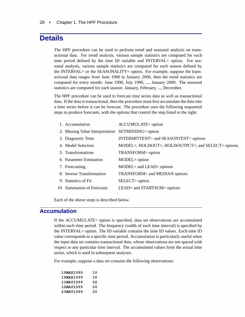
The HPF procedure can be used to perform trend and seasonal analysis on trans-actional data. For trend analysis, various sample statistics are computed for eachtime period defined by the time ID variable and INTERVAL= option. For sea-sonal analysis, various sample statistics are computed for each season defined bythe INTERVAL= or the SEASONALITY= option. For example, suppose the trans-actional data ranges from June 1990 to January 2000, then the trend statistics arecomputed for every month: June 1990, July 1990, ..., January 2000. The seasonalstatistics are computed for each season: January, February, ..., December.
The HPF procedure can be used to forecast time series data as well as transactionaldata. If the data is transactional, then the procedure must first accumulate the data intoa time series before it can be forecast. The procedure uses the following sequentialsteps to produce forecasts, with the options that control the step listed to the right:
1. Accumulation ACCUMULATE= option
2. Missing Value InterpretationSETMISSING= option
3. Diagnostic Tests INTERMITTENT= and SEASONTEST= options
4. Model Selection MODEL=, HOLDOUT=, HOLDOUTPCT=, and SELECT= options
5. Transformations TRANSFORM= option
6. Parameter Estimation MODEL= option
7. Forecasting MODEL= and LEAD= options
8. Inverse Transformation TRANSFORM= and MEDIAN options
9. Statistics of Fit SELECT= option
10. Summation of Forecasts LEAD= and STARTSUM= options
Each of the above steps is described below.
Accumulation
If the ACCUMULATE= option is specified, data set observations are accumulatedwithin each time period. The frequency (width of each time interval) is specified bythe INTERVAL= option. The ID variable contains the time ID values. Each time IDvalue corresponds to a specific time period. Accumulation is particularly useful whenthe input data set contains transactional data, whose observations are not spaced withrespect to any particular time interval. The accumulated values form the actual timeseries, which is used in subsequent analyses.
For example, suppose a data set contains the following observations:
19MAR1999 1019MAR1999 3011MAY1999 5012MAY1999 2023MAY1999 20
Accumulation � 29
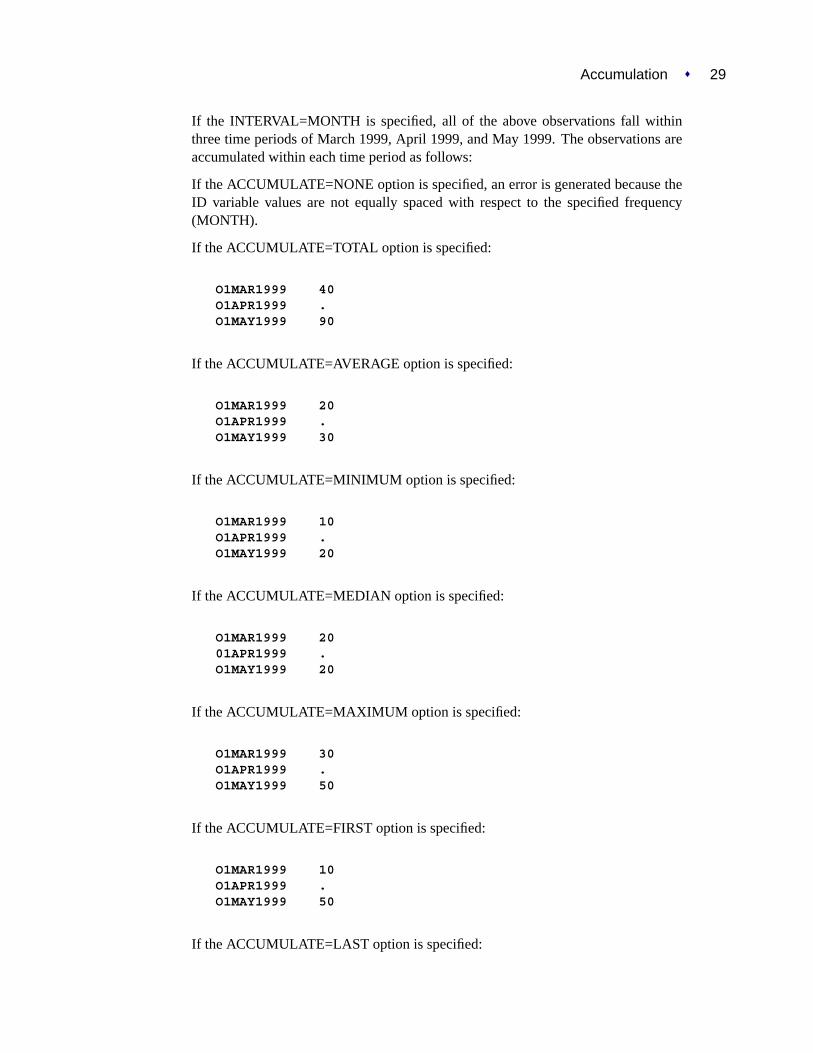
If the INTERVAL=MONTH is specified, all of the above observations fall withinthree time periods of March 1999, April 1999, and May 1999. The observations areaccumulated within each time period as follows:
If the ACCUMULATE=NONE option is specified, an error is generated because theID variable values are not equally spaced with respect to the specified frequency(MONTH).
If the ACCUMULATE=TOTAL option is specified:
O1MAR1999 40O1APR1999 .O1MAY1999 90
If the ACCUMULATE=AVERAGE option is specified:
O1MAR1999 20O1APR1999 .O1MAY1999 30
If the ACCUMULATE=MINIMUM option is specified:
O1MAR1999 10O1APR1999 .O1MAY1999 20
If the ACCUMULATE=MEDIAN option is specified:
O1MAR1999 2001APR1999 .O1MAY1999 20
If the ACCUMULATE=MAXIMUM option is specified:
O1MAR1999 30O1APR1999 .O1MAY1999 50
If the ACCUMULATE=FIRST option is specified:
O1MAR1999 10O1APR1999 .O1MAY1999 50
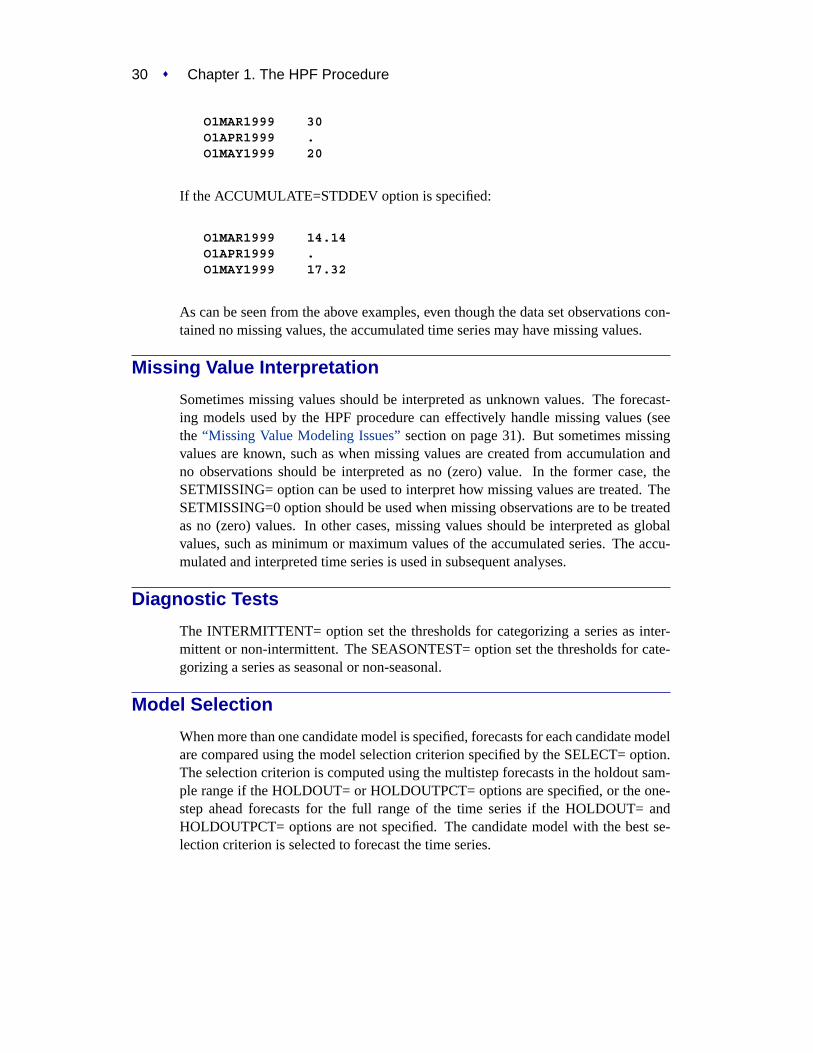
If the ACCUMULATE=LAST option is specified:
30 � Chapter 1. The HPF Procedure
O1MAR1999 30O1APR1999 .O1MAY1999 20
If the ACCUMULATE=STDDEV option is specified:
O1MAR1999 14.14O1APR1999 .O1MAY1999 17.32
As can be seen from the above examples, even though the data set observations con-tained no missing values, the accumulated time series may have missing values.
Missing Value Interpretation
Sometimes missing values should be interpreted as unknown values. The forecast-ing models used by the HPF procedure can effectively handle missing values (seethe “Missing Value Modeling Issues”section on page 31). But sometimes missingvalues are known, such as when missing values are created from accumulation andno observations should be interpreted as no (zero) value. In the former case, theSETMISSING= option can be used to interpret how missing values are treated. TheSETMISSING=0 option should be used when missing observations are to be treatedas no (zero) values. In other cases, missing values should be interpreted as globalvalues, such as minimum or maximum values of the accumulated series. The accu-mulated and interpreted time series is used in subsequent analyses.
Diagnostic Tests
The INTERMITTENT= option set the thresholds for categorizing a series as inter-mittent or non-intermittent. The SEASONTEST= option set the thresholds for cate-gorizing a series as seasonal or non-seasonal.
Model Selection
When more than one candidate model is specified, forecasts for each candidate modelare compared using the model selection criterion specified by the SELECT= option.The selection criterion is computed using the multistep forecasts in the holdout sam-ple range if the HOLDOUT= or HOLDOUTPCT= options are specified, or the one-step ahead forecasts for the full range of the time series if the HOLDOUT= andHOLDOUTPCT= options are not specified. The candidate model with the best se-lection criterion is selected to forecast the time series.
Inverse Transformations � 31
Transformations
If the TRANSFORM= option is specified, the time series is transformed prior tomodel parameter estimation and forecasting. Only strictly positive series can betransformed. An error is generated when the TRANSFORM= option is used witha nonpositive series.
Parameter Estimation
All parameters associated with the model are optimized based on the data with thedefault parameter restrictions imposed. If the TRANSFORM= option is specified,the transformed time series data are used to estimate the model parameters.
Missing Value Modeling Issues
The treatment of missing values varies with the forecasting model. For the smoothingmodels, missing values after the start of the series are replaced with one-step-aheadpredicted values, and the predicted values are applied to the smoothing equations. SeeChapter 2, “Forecasting Process Details,”for greater detail on how missing valuesare treated in the smoothing models. For MODEL=IDM, specified missing valuesare assumed to be periods of no demand.
The treatment of missing values can also be specified by the user with theSETMISSING= option, which changes the missing values prior to modeling.
Even though all of the observed data are nonmissing, using the ACCUMULATE=option can create missing values in the accumulated series.
Forecasting
Once the model parameters are estimated, one-step ahead forecasts are generated forthe full range of the actual (optionally transformed) time series data, and multistepforecasts are generated from the end of the observed time series to the future timeperiod after the last observation specified by the LEAD= option. If there are missingvalues at the end of the time series, the forecast horizon will be greater than thatspecified by the LEAD= option.
Inverse Transformations
If the TRANSFORM= option is specified, the forecasts of the transformed time seriesare inverse transformed. By default, the mean (expected) forecasts are generated. Ifthe MEDIAN option is specified, the median forecasts are generated.
32 � Chapter 1. The HPF Procedure
Statistics of Fit
The statistics of fit (or goodness-of-fit statistics) are computed by comparing the ac-tual time series data and the generated forecasts. If the TRANSFORM= option wasspecified, the statistics of fit are based on the inverse transformed forecasts.
Forecast Summation
The multistep forecasts generated by the above steps are summed from theSTARTSUM= number to the LEAD= number. For example, if STARTSUM=4 andLEAD=6, the 4-step through 6-step ahead forecasts are summed. The predictionsare simply summed. However, the prediction error variance of this sum is computedtaking into account the correlation between the individual predictions. The upperand lower confidence limits for the sum of the predictions is then computed based onthe prediction error variance of the sum.
The forecast summation is particularly useful when it is desirable to model in onefrequency yet the forecast of interest is another frequency. For example, if a timeseries has a monthly frequency (INTERVAL=MONTH) and you want a forecast forthe third and fourth future months, a forecast summation for the third and fourthmonth can be obtained by specifying STARTSUM=3 and LEAD=4.
Variance-related computations are only computed when no transformation is speci-fied (TRANSFORM=NONE).
Comparison to the Time Series Forecasting System
With the exception of Model Selection, the techniques used in the HPF procedure areidentical to the Time Series Forecasting System of SAS/ETS software. For ModelParameter Estimation, the default parameter restrictions are imposed.
Data Set Output
The HPF procedure can create the OUT=, OUTEST=, OUTFOR=, OUTSTAT=,OUTSUM=, OUTSEASON=, and OUTTREND= data sets. In general, these datasets will contain the variables listed in the BY statement. In general, if a forecastingstep related to an output data step fails, the values of this step are not recorded orare set to missing in the related output data set, and appropriate error and/or warningmessages are recorded in the log.
OUT= Data Set
The OUT= data set contains the variables specified in the BY, ID, and FORECASTstatements. If the ID statement is specified, the ID variable values are alignedand extended based on the ALIGN= and INTERVAL= options. The values ofthe variables specified in the FORECAST statements are accumulated based onthe ACCUMULATE= option and missing values are interpreted based on theSETMISSING= option. If the REPLACEMISSING option is specified, missing val-ues embedded missing values are replaced by the one step-ahead forecasts.
OUTFOR= Data Set � 33
These variable values are then extrapolated based on their forecasts or extended withmissing values when the MODEL=NONE option is specified. If USE=LOWERis specified, the variable is extrapolated with the lower confidence limits; ifUSE=UPPER, the variable is extrapolated using the upper confidence limits; oth-erwise, the variable values are extrapolated with the predicted values. If theTRANSFORM= option is specified, the predicted values will contain either meanor median forecasts depending on whether or not the MEDIAN option is specified.
If any of the forecasting steps fail for particular variable, the variable values are ex-tended by missing values.
OUTEST= Data Set
The OUTEST= data set contains the variables specified in the BY statement as wellas the variables listed below. For variables listed in FORECAST statements where theoption MODEL=NONE is specified, no observations are recorded for these variables.For variables listed in FORECAST statements where the option MODEL=NONE isnot specified, the following variables contain observations related to the parameterestimation step:
–NAME– Variable name
–MODEL– Forecasting Model
–TRANSFORM– Transformation
–PARM– Parameter Name
–EST– Parameter Estimate
–STDERR– Standard Errors
–TVALUE– t-Values
–PVALUE– Probability Values
If the parameter estimation step fails for a particular variable, no observations arerecorded.
OUTFOR= Data Set
The OUTFOR= data set contains the variables specified in the BY statement as wellas the variables listed below. For variables listed in FORECAST statements where theoption MODEL=NONE is specified, no observations are recorded for these variables.For variables listed in FORECAST statements where the option MODEL=NONE isnot specified, the following variables contain observations related to the forecastingstep:
–NAME– Variable name
–TIMEID– Time ID values
PREDICT Predicted Values
STD Prediction Standard Errors
34 � Chapter 1. The HPF Procedure
LOWER Lower Confidence Limits
UPPER Upper Confidence Limits
ERROR Prediction Errors
If the forecasting step fails for a particular variable, no observations are recorded.If the TRANSFORM= option is specified, the values in the variables listed aboveare the inverse transform forecasts. If the MEDIAN option is specified, the medianforecasts are stored; otherwise, the mean forecasts are stored.
OUTSTAT= Data Set
The OUTSTAT= data set contains the variables specified in the BY statement as wellas the variables listed below. For variables listed in FORECAST statements where theoption MODEL=NONE is specified, no observations are recorded for these variables.For variables listed in FORECAST statements where the option MODEL=NONE isnot specified, the following variables contain observations related to the statistics offit step:
–NAME– Variable name
SSE Sum of Square Error
MSE Mean Square Error
UMSE Unbiased Mean Square Error
RMSE Root Mean Square Error
URMSE Unbiased Root Mean Square Error
MAPE Mean Absolute Percent Error
MAE Mean Absolute Error
RSQUARE R-Square
ADJRSQ Adjusted R-Square
AADJRSQ Amemiya’s Adjusted R-Square
RWRSQ Random Walk R-Square
AIC Akaike Information Criterion
SBC Schwarz Bayesian Information Criterion
APC Amemiya’s Prediction Criterion
MAXERR Maximum Error
MINERR Minimum Error
MINPE Maximum Percent Error
MAXPE Minimum Percent Error
ME Mean Error
MPE Mean Percent Error
OUTSUM= Data Set � 35
If the statistics of fit step fails for particular variable, no observations are recorded.If the TRANSFORM= option is specified, the values in the variables listed aboveare computed based on the inverse transform forecasts. If the MEDIAN option isspecified, the median forecasts are the basis; otherwise, the mean forecasts are thebasis.
OUTSUM= Data Set
The OUTSUM= data set contains the variables specified in the BY statement as wellas the variables listed below. The OUTSUM= data set records the summary statis-tics for each variable specified in a FORECAST statement. For variables listed inFORECAST statements where the option MODEL=NONE is specified, the valuesrelated to forecasts are set to missing. For variables listed in FORECAST statementswhere the option MODEL=NONE is not specified, the forecast values are set basedon the USE= option.
Variables related to summary statistics are based on the ACCUMULATE= andSETMISSING= options:
–NAME– Variable name
–STATUS– Forecasting Status. Nonzero values imply that no forecast was gen-erated for the series.
NOBS Number of Observations
N Number of Nonmissing Observations
NMISS Number of Missing Observations
MIN Minimum Value
MAX Maximum Value
MEAN Mean Value
STDDEV Standard Deviation
Variables related to forecast summation are based on the LEAD= and STARTSUM=options:
PREDICT Forecast Summation Predicted Values
STD Forecast Summation Prediction Standard Errors
LOWER Forecast Summation Lower Confidence Limits
UPPER Forecast Summation Upper Confidence Limits
Variance-related computations are only computed when no transformation is speci-fied (TRANSFORM=NONE).
Variables related to multistep forecast based on the LEAD= and USE= options:
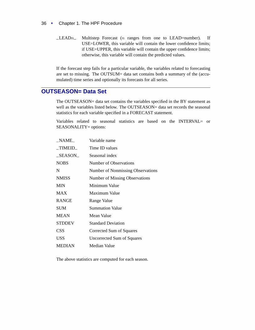
36 � Chapter 1. The HPF Procedure
–LEADn– Multistep Forecast (n ranges from one to LEAD=number). IfUSE=LOWER, this variable will contain the lower confidence limits;if USE=UPPER, this variable will contain the upper confidence limits;otherwise, this variable will contain the predicted values.
If the forecast step fails for a particular variable, the variables related to forecastingare set to missing. The OUTSUM= data set contains both a summary of the (accu-mulated) time series and optionally its forecasts for all series.
OUTSEASON= Data Set
The OUTSEASON= data set contains the variables specified in the BY statement aswell as the variables listed below. The OUTSEASON= data set records the seasonalstatistics for each variable specified in a FORECAST statement.
Variables related to seasonal statistics are based on the INTERVAL= orSEASONALITY= options:
–NAME– Variable name
–TIMEID– Time ID values
–SEASON– Seasonal index
NOBS Number of Observations
N Number of Nonmissing Observations
NMISS Number of Missing Observations
MIN Minimum Value
MAX Maximum Value
RANGE Range Value
SUM Summation Value
MEAN Mean Value
STDDEV Standard Deviation
CSS Corrected Sum of Squares
USS Uncorrected Sum of Squares
MEDIAN Median Value
The above statistics are computed for each season.
Printed Output � 37
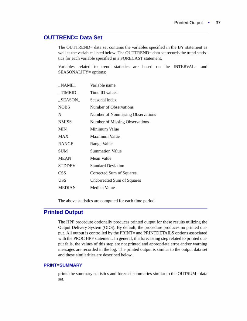
OUTTREND= Data Set
The OUTTREND= data set contains the variables specified in the BY statement aswell as the variables listed below. The OUTTREND= data set records the trend statis-tics for each variable specified in a FORECAST statement.
Variables related to trend statistics are based on the INTERVAL= andSEASONALITY= options:
–NAME– Variable name
–TIMEID– Time ID values
–SEASON– Seasonal index
NOBS Number of Observations
N Number of Nonmissing Observations
NMISS Number of Missing Observations
MIN Minimum Value
MAX Maximum Value
RANGE Range Value
SUM Summation Value
MEAN Mean Value
STDDEV Standard Deviation
CSS Corrected Sum of Squares
USS Uncorrected Sum of Squares
MEDIAN Median Value
The above statistics are computed for each time period.
Printed Output
The HPF procedure optionally produces printed output for these results utilizing theOutput Delivery System (ODS). By default, the procedure produces no printed out-put. All output is controlled by the PRINT= and PRINTDETAILS options associatedwith the PROC HPF statement. In general, if a forecasting step related to printed out-put fails, the values of this step are not printed and appropriate error and/or warningmessages are recorded in the log. The printed output is similar to the output data setand these similarities are described below.
PRINT=SUMMARY
prints the summary statistics and forecast summaries similar to the OUTSUM= dataset.

38 � Chapter 1. The HPF Procedure
PRINT=ESTIMATES
prints the parameter estimates similar to the OUTEST= data set.
PRINT=FORECASTS
prints the forecasts similar to the OUTFOR= data set. For MODEL=IDM, a tablecontaining demand series is also printed.
If the MODEL=IDM option is specified, the demand series predictions table is alsoprinted. This table is based on the demand index (when demands occurred).
PRINT=PERFORMANCE
prints the performance statistics.
PRINT=PERFORMANCESUMMARY
prints the performance summary for each BY group.
PRINT=PERFORMANCEOVERALL
prints the performance summary for all BY groups.
PRINT=STATES
prints the backcast, initial, and final smoothed states.
PRINT=SEASONS
prints the seasonal statistics similar to the OUTSEASON= data set.
PRINT=STATISTICS
prints the statistics of fit similar to the OUTSTAT= data set.
PRINT=TRENDS
Prints the trend statistics similar to the OUTTREND= data set.
PRINTDETAILS
The PRINTDETAILS option is the opposite of the NOOUTALL option.
Specifically, if PRINT=FORECASTS and the PRINTDETAILS options are specified,the one-step ahead forecasts, throughout the range of the data, are printed as well asthe information related to a specific forecasting model such as the smoothing states. Ifthe PRINTDETAILS option is not specified, only the multistep forecasts are printed.

ODS Graphics (Experimental) � 39
ODS Table Names
The table below relates the PRINT= options to ODS tables:
Table 1.1. ODS Tables Produced in PROC HPF
ODS Table Name Description Option
ODS Tables Created by the PRINT=SUMMARY optionDescStats Descriptive StatisticsDemandSummary Demand Summary MODEL=IDM option onlyForecastSummary Forecast SummaryForecastSummmation Forecast Summation
ODS Tables Created by the PRINT=ESTIMATES optionModelSelection Model SelectionParameterEstimates Parameter Estimates
ODS Tables Created by the PRINT=FORECASTS optionForecasts ForecastDemands Demands MODEL=IDM option only
ODS Tables Created by the PRINT=PERFORMANCE optionPerformance Performance Statistics
ODS Tables Created by the PRINT=PERFORMANCESUMMARY optionPerformanceSummary Performance Summary
ODS Tables Created by the PRINT=PERFORMANCEOVERALL optionPerformanceSummary Performance Overall
ODS Tables Created by the PRINT=SEASONS optionSeasonStatistics Seasonal Statistics
ODS Tables Created by the PRINT=STATES optionSmoothedStates Smoothed StatesDemandStates Demand States MODEL=IDM option only
ODS Tables Created by the PRINT=STATISTICS optionFitStatistics Statistics of Fit
ODS Tables Created by the PRINT=TRENDS optionTrendStatistics Trend Statistics
The ODS table ForecastSummary is related to all time series within a BY group. Theother tables are related to a single series within a BY group.
ODS Graphics (Experimental)
This section describes the use of ODS for creating graphics with the HPF procedure.These graphics are experimental in this release, meaning that both the graphical re-sults and the syntax for specifying them are subject to change in a future release.
To request these graphs, you must specify the ODS GRAPHICS statement. In ad-dition, you can specify thePLOT= option in the HPF statement according to the

40 � Chapter 1. The HPF Procedure
following syntax. For more information on the ODS GRAPHICS statement, refer toChapter 9, “Statistical Graphics Using ODS” (SAS/ETS User’s Guide).
PLOT= option | (options)specifies the graphical output desired. By default, the HPF procedure produces nographical output. The following printing options are available:
ERRORS plots prediction error time series graphics.
ACF plots prediction error autocorrelation function graphics.
PACF plots prediction error partial autocorrelation function graphics.
IACF plots prediction error inverse autocorrelation function graphics.
WN plots white noise graphics.
MODELS plots model graphics.
FORECASTS plots forecast graphics.
MODELFORECASTSONLY plots forecast graphics with confidence limits in thedata range.
FORECASTSONLY plots the forecast in the forecast horzion only.
LEVELS plots smoothed level component graphics.
SEASONS plots smoothed seasonal component graphics.
TRENDS plots smoothed trend (slope) component graphics.
ALL Same as specifying all of the above PLOT= options.
For example, PLOT=FORECASTS plots the forecasts for each series. The PLOT=option produces printed output for these results utilizing the Output Delivery System(ODS). The PLOT= statement is experimental for this release of SAS.
ODS Graph Names
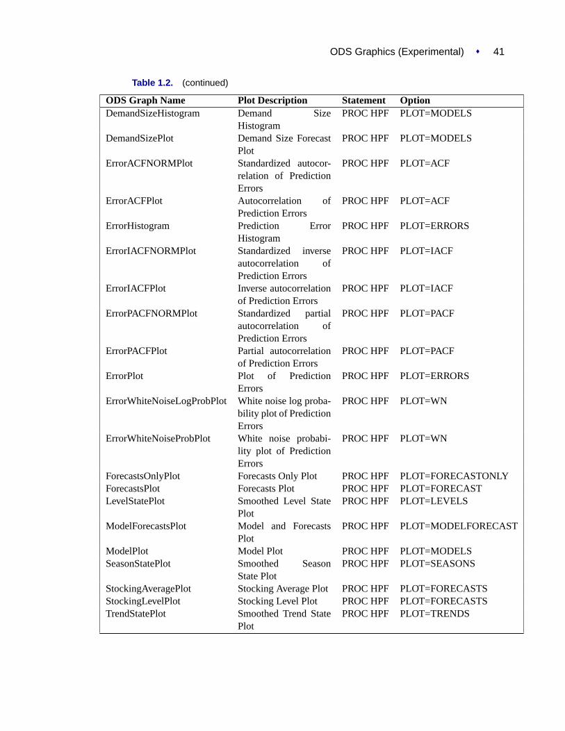
PROC HPF assigns a name to each graph it creates using ODS. You can use thesenames to reference the graphs when using ODS. The names are listed inTable 1.2.
To request these graphs, you must specify the ODS GRAPHICS statement. In addi-tion, you can specify thePLOT= option in the HPF statement. For more informationon the ODS GRAPHICS statement, refer to Chapter 9, “Statistical Graphics UsingODS” (SAS/ETS User’s Guide).
Table 1.2. ODS Graphics Produced by PROC HPF
ODS Graph Name Plot Description Statement PLOT= OptionDemandErrorsPlot Average Demand
ErrorsPROC HPF PLOT=ERRORS
DemandForecastsPlot Average DemandForecasts
PROC HPF PLOT=FORECASTS
DemandIntervalHistogram Demand IntervalHistogram
PROC HPF PLOT=MODELS
DemandIntervalPlot Demand IntervalForecast Plot
PROC HPF PLOT=MODELS
ODS Graphics (Experimental) � 41
Table 1.2. (continued)
ODS Graph Name Plot Description Statement OptionDemandSizeHistogram Demand Size
HistogramPROC HPF PLOT=MODELS
DemandSizePlot Demand Size ForecastPlot
PROC HPF PLOT=MODELS
ErrorACFNORMPlot Standardized autocor-relation of PredictionErrors
PROC HPF PLOT=ACF
ErrorACFPlot Autocorrelation ofPrediction Errors
PROC HPF PLOT=ACF
ErrorHistogram Prediction ErrorHistogram
PROC HPF PLOT=ERRORS
ErrorIACFNORMPlot Standardized inverseautocorrelation ofPrediction Errors
PROC HPF PLOT=IACF
ErrorIACFPlot Inverse autocorrelationof Prediction Errors
PROC HPF PLOT=IACF
ErrorPACFNORMPlot Standardized partialautocorrelation ofPrediction Errors
PROC HPF PLOT=PACF
ErrorPACFPlot Partial autocorrelationof Prediction Errors
PROC HPF PLOT=PACF
ErrorPlot Plot of PredictionErrors
PROC HPF PLOT=ERRORS
ErrorWhiteNoiseLogProbPlot White noise log proba-bility plot of PredictionErrors
PROC HPF PLOT=WN
ErrorWhiteNoiseProbPlot White noise probabi-lity plot of PredictionErrors
PROC HPF PLOT=WN
ForecastsOnlyPlot Forecasts Only Plot PROC HPF PLOT=FORECASTONLYForecastsPlot Forecasts Plot PROC HPF PLOT=FORECASTLevelStatePlot Smoothed Level State
PlotPROC HPF PLOT=LEVELS
ModelForecastsPlot Model and ForecastsPlot
PROC HPF PLOT=MODELFORECAST
ModelPlot Model Plot PROC HPF PLOT=MODELSSeasonStatePlot Smoothed Season
State PlotPROC HPF PLOT=SEASONS
StockingAveragePlot Stocking Average Plot PROC HPF PLOT=FORECASTSStockingLevelPlot Stocking Level Plot PROC HPF PLOT=FORECASTSTrendStatePlot Smoothed Trend State
PlotPROC HPF PLOT=TRENDS

42 � Chapter 1. The HPF Procedure
Examples
Example 1.1. Automatic Forecasting of Time Series Data
This example illustrates how the HPF procedure can be used for the automatic fore-casting of time series data. Retail sales data is used for this illustration.
The following DATA step creates a data set from data recorded monthly at numerouspoints of sales. The data set,SALES, will contain a variableDATE that representstime and a variable for each sales item. Each value of theDATE variable is recordedin ascending order and the values of each of the other variables represent a singletime series:
data sales;format date date9.;input date date9. shoes socks laces dresses coats shirts ties
belts hats blouses;datalines;... data lines omitted ...;
run;
The following HPF procedure statements automatically forecast each of the monthlytime series.
proc hpf data=sales out=nextyear;id date interval=month;forecast _ALL_;
run;
The above statements automatically select the best fitting model and generate fore-casts for every numeric variable in the input data set (SALES) for the next twelvemonths, and stores these forecasts in the output data set (NEXTYEAR).
The following GPLOT procedure statements plot the forecasts related to shoe sales:
title1 "Shoe Department Sales";axis2 label=(a=-90 r=90 "items" );symbol1 v = dot i = join l = 1;symbol2 v = star i = join l = 2;symbol3 v = circle i = join l = 2;
proc gplot data=nextyear;plot shoes * date = 1
socks * date = 2laces * date = 3 / overlayhaxis= ’01JAN1994’d to ’01DEC2000’d by yearhref= ’01JAN1999’dvaxis=axis2;
run;

Example 1.2. Automatic Forecasting of Time Series Data � 43
The GPLOT procedure results are shown inFigure 1.1. The historical data is shownleft the horizontal reference line and the forecasts for the next twelve monthly periodsis shown to the right.
Figure 1.1. Retail Sales Forecast Plots
The following HPF procedure statements are identical to the statements above withthe exception that the PRINT=FORECASTS option is specified:
proc hpf data=sales out=nextyear print=forecasts;id date interval=month;forecast _ALL_;
run;
In addition to automatically forecasting each of the monthly time series, the abovestatements print the forecasts using the Output Delivery System (ODS), which is par-tially shown inOutput 1.1.1. This output shows the predictions, prediction standarderrors and the upper and lower confidence limits for the next twelve monthly periods.

44 � Chapter 1. The HPF Procedure
Output 1.1.1. Forecast TablesForecasts for Variable shoes
StandardObs Time Forecasts Error 95% Confidence Limits
62 FEB1999 7548.0041 607.5238 6357.2792 8738.728963 MAR1999 7177.1472 699.4400 5806.2701 8548.024464 APR1999 5497.5595 780.7609 3967.2964 7027.822765 MAY1999 4838.2001 854.5169 3163.3778 6513.022466 JUN1999 6728.4521 922.5244 4920.3375 8536.566867 JUL1999 6786.1094 985.9738 4853.6362 8718.582668 AUG1999 5853.9650 1045.6953 3804.4399 7903.490069 SEP1999 7517.0144 1102.2949 5356.5561 9677.472870 OCT1999 7100.2489 1156.2315 4834.0769 9366.421071 NOV1999 7224.6449 1207.8618 4857.2793 9592.010672 DEC1999 6357.1556 1257.4701 3892.5594 8821.751873 JAN2000 6492.2657 1305.2871 3933.9500 9050.5815
Example 1.2. Automatic Forecasting of Transactional Data
This example illustrates how the HPF procedure can be used to automatically forecasttransactional data. Internet data is used for this illustration.
The following DATA step creates a data set from data recorded at several Internet Websites. The data set,WEBSITES, will contain a variable TIME that represents timeand the variables ENGINE,BOATS, CARS, andPLANES that represent InternetWeb site data. Each value of the TIME variable is recorded in ascending order, andthe values of each of the other variables represent a transactional data series.
data websites;format time datetime.;input time datetime. boats cars planes engines;datalines;... data lines omitted ...;
run;
The following HPF procedure statements automatically forecast each of the transac-tional data series:
proc hpf data=websites out=nextweek lead=7;id time interval=dtday accumulate=total;forecast boats cars planes;
run;
The above statements accumulate the data into a daily time series and automaticallygenerate forecasts for theBOATS, CARS, andPLANES variables in the input dataset (WEBSITES) for the next week and stores the forecasts in the output data set(NEXTWEEK).
The following GPLOT procedure statements plot the forecasts related to the Internetdata:

Example 1.3. Specifying the Forecasting Model � 45
title1 "Website Data";axis2 label=(a=-90 r=90 "Websites" );symbol1 v = dot i = join l = 1;symbol2 v = star i = join l = 2;symbol3 v = circle i = join l = 2;
proc gplot data=nextweek;plot boats * time = 1
cars * time = 2planes * time = 3 / overlayhaxis= ’13MAR2000:00:00:00’dt to
’18APR2000:00:00:00’dt by dtweekhref= ’11APR2000:00:00:00’dtvaxis=axis2;
run;
The GPLOT procedure results are shown inFigure 1.2. The historical data is shown tothe left of the horizontal reference line and the forecasts for the next twelve monthlyperiods are shown to the right.
Figure 1.2. Internet Data Forecast Plots
Example 1.3. Specifying the Forecasting Model
In the previous example, the HPF procedure was used to automatically select theappropriate forecasting model using the root mean square error (RMSE) as the defaultselection criterion. This example illustrates how the HPF procedure can be used tomore narrowly specify the possible candidate models. Internet data from the previousexample are used for this illustration.

46 � Chapter 1. The HPF Procedure
In this example, we will forecast theBOATS variable using the best seasonal fore-casting model (BESTS) that minimizes the mean absolute percent error (MAPE), theCARS variable using the best nonseasonal forecasting model (BESTN) that mini-mizes the mean square error (MSE) using holdout sample analysis, and thePLANESvariable using Log Winters (additive). The following HPF procedure statements fore-cast each of the transactional data series based on these requirements:
proc hpf data=websites out=nextweek lead=7;id time interval=dtday accumulate=total;forecast boats / model=bests select=mape;forecast cars / model=bestn select=mse holdout=5;forecast planes / model=addwinters transform=log;
run;
Example 1.4. Extending the Independent Variables forMultivariate Forecasts
In the previous example, the HPF procedure was used to forecast several transac-tional series variables using univariate models. This example illustrates how the HPFprocedure can be used to extend the independent variables associated with a multi-ple regression forecasting problem. Specifically, PROC HPF is used to extend theindependent variables for use in forecasting a regression model.
In this example, we will accumulate and forecast theBOATS, CARS, andPLANESvariables as illustrated in the previous example. In addition, we will accumulate theENGINES variable to form a time series that is then extended with missing valueswithin the forecast horizon with the specification of MODEL=NONE.
proc hpf data=websites out=nextweek lead=7;id time interval=dtday accumulate=total;forecast engines / model=none;forecast boats / model=bests select=mape;forecast cars / model=bestn select=mse holdout=5;forecast planes / model=winters transform=log;
run;
The following AUTOREG procedure statements are used to forecast the ENGINESvariable by regressing on the independent variables (BOATS, CARS, andPLANES).
proc autoreg data= nextweek;model engines = boats cars planes / noprint;output out=enginehits p=predicted;
run;
The output data set (NEXTWEEK) of the PROC HPF statement is used as an in-put data set for the PROC AUTOREG statement. The output data set of PROCAUTOREG contains the forecast of the variable ENGINES based on the regres-sion model with the variablesBOATS, CARS, andPLANES as regressors. Seethe AUTOREG procedure for details on autoregression models.

Example 1.5. Forecasting Intermittent Time Series Data � 47
The following GPLOT procedure statements plot the forecasts related to theENGINES variable:
proc gplot data=enginehits;plot boats * time = 1
cars * time = 2planes * time = 3predicted * time = 4 / overlayhaxis= ’13MAR2000:00:00:00’dt to
’18APR2000:00:00:00’dt by dtweekhref= ’11APR2000:00:00:00’dtvaxis=axis2;
run;
The GPLOT procedure results are shown inFigure 1.3. The historical data is shownleft the horizontal reference line and the forecasts for the next four weekly periods isshown to the right.
Figure 1.3. Internet Data Forecast Plots
Example 1.5. Forecasting Intermittent Time Series DataThis example illustrates how the HPF procedure can be used to forecast intermittenttime series data. Inventory demand is used for this illustration.
The following DATA step creates a data set from inventory data recorded at no par-ticular frequency. The data set,INVENTORY, will contain a variableDATE thatrepresents time and the demand variables (TIRES, HUBCAPS, andLUGBOLTS),which represent inventory items. Each value of theDATE variable is recorded in as-cending order, and the values of each of the other variables represent a transactionaldata series.
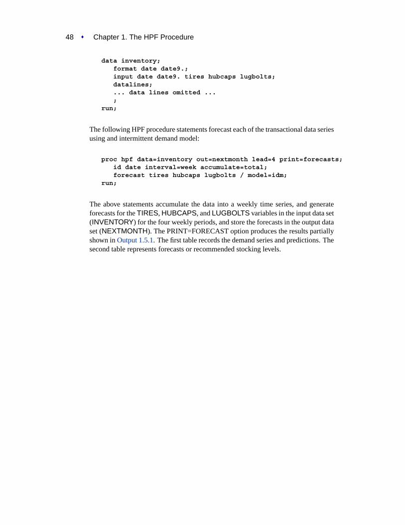
48 � Chapter 1. The HPF Procedure
data inventory;format date date9.;input date date9. tires hubcaps lugbolts;datalines;... data lines omitted ...;
run;
The following HPF procedure statements forecast each of the transactional data seriesusing and intermittent demand model:
proc hpf data=inventory out=nextmonth lead=4 print=forecasts;id date interval=week accumulate=total;forecast tires hubcaps lugbolts / model=idm;
run;
The above statements accumulate the data into a weekly time series, and generateforecasts for theTIRES, HUBCAPS, andLUGBOLTS variables in the input data set(INVENTORY) for the four weekly periods, and store the forecasts in the output dataset (NEXTMONTH). The PRINT=FORECAST option produces the results partiallyshown inOutput 1.5.1. The first table records the demand series and predictions. Thesecond table represents forecasts or recommended stocking levels.
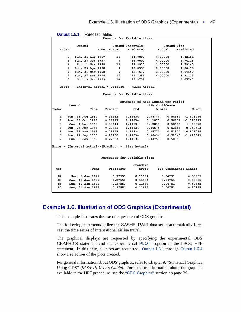
Example 1.6. Illustration of ODS Graphics (Experimental) � 49
Output 1.5.1. Forecast TablesDemands for Variable tires
Demand Demand Intervals Demand SizeIndex Time Actual Predicted Actual Predicted
1 Sun, 31 Aug 1997 14 14.0000 6.00000 4.421512 Sun, 26 Oct 1997 8 14.0000 4.00000 4.742163 Sun, 1 Mar 1998 18 12.8920 2.00000 4.591404 Sun, 26 Apr 1998 8 13.8353 2.00000 4.064985 Sun, 31 May 1998 5 12.7577 2.00000 3.645506 Sun, 27 Sep 1998 17 11.3251 6.00000 3.311237 Sun, 3 Jan 1999 14 12.3731 . 3.85743
Error = (Interval Actual)*(Predict) - (Size Actual)
Demands for Variable tires
Estimate of Mean Demand per PeriodDemand 95% Confidence
Index Time Predict Std Limits Error
1 Sun, 31 Aug 1997 0.31582 0.11634 0.08780 0.54384 -1.5784942 Sun, 26 Oct 1997 0.33873 0.11634 0.11071 0.56674 -1.2901933 Sun, 1 Mar 1998 0.35614 0.11634 0.12813 0.58416 4.4105784 Sun, 26 Apr 1998 0.29381 0.11634 0.06579 0.52183 0.3505035 Sun, 31 May 1998 0.28575 0.11634 0.05773 0.51377 -0.5712546 Sun, 27 Sep 1998 0.29238 0.11634 0.06436 0.52040 -1.0295437 Sun, 3 Jan 1999 0.27553 0.11634 0.04751 0.50355 .
Error = (Interval Actual)*(Predict) - (Size Actual)
Forecasts for Variable tires
StandardObs Time Forecasts Error 95% Confidence Limits
84 Sun, 3 Jan 1999 0.27553 0.11634 0.04751 0.5035585 Sun, 10 Jan 1999 0.27553 0.11634 0.04751 0.5035586 Sun, 17 Jan 1999 0.27553 0.11634 0.04751 0.5035587 Sun, 24 Jan 1999 0.27553 0.11634 0.04751 0.50355
Example 1.6. Illustration of ODS Graphics (Experimental)
This example illustrates the use of experimental ODS graphics.
The following statements utilize theSASHELP.AIR data set to automatically fore-cast the time series of international airline travel.
The graphical displays are requested by specifying the experimental ODSGRAPHICS statement and the experimentalPLOT= option in the PROC HPFstatement. In this case, all plots are requested.Output 1.6.1throughOutput 1.6.4show a selection of the plots created.
For general information about ODS graphics, refer to Chapter 9, “Statistical GraphicsUsing ODS” (SAS/ETS User’s Guide). For specific information about the graphicsavailable in the HPF procedure, see the“ODS Graphics”section on page 39.

50 � Chapter 1. The HPF Procedure
ods html;ods graphics on;
proc hpf data=sashelp.air out=_null_ lead=20 back=20 print=all plot=all;id date interval=month;
forecast air / model=best transform=auto select=mape;run;
ods graphics off;ods html close;
Output 1.6.1. Smoothed Trend Plot (Experimental)
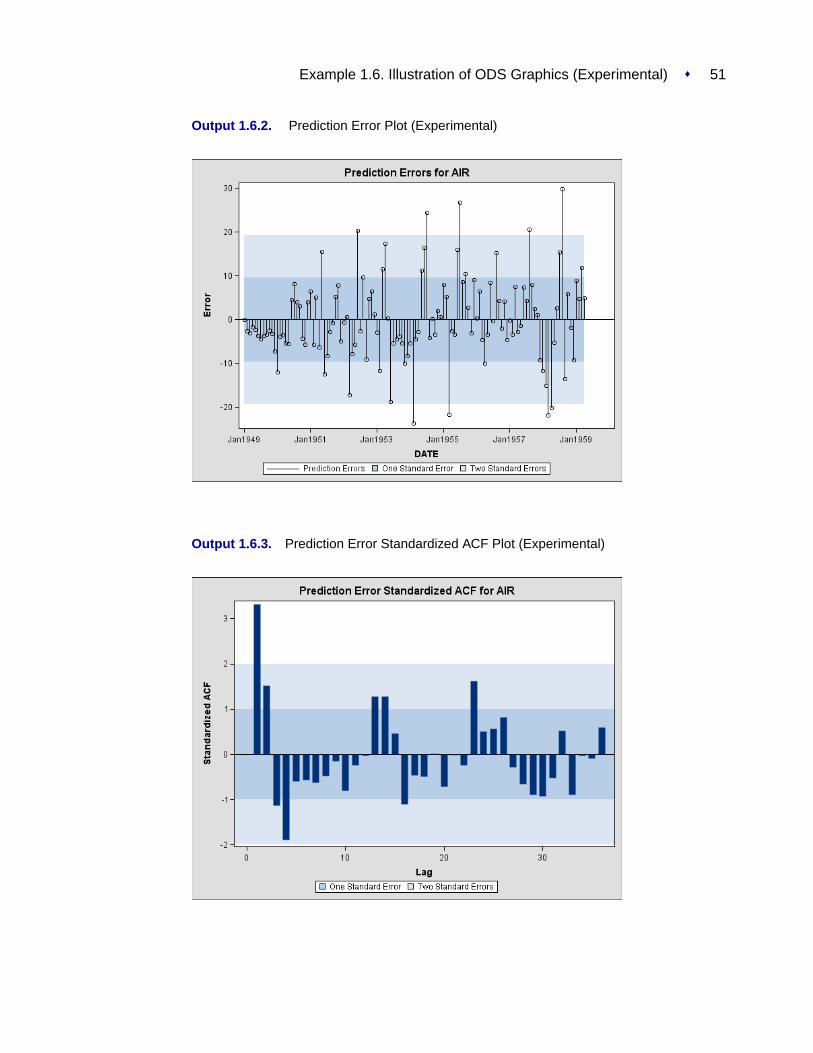
Example 1.6. Illustration of ODS Graphics (Experimental) � 51
Output 1.6.2. Prediction Error Plot (Experimental)
Output 1.6.3. Prediction Error Standardized ACF Plot (Experimental)
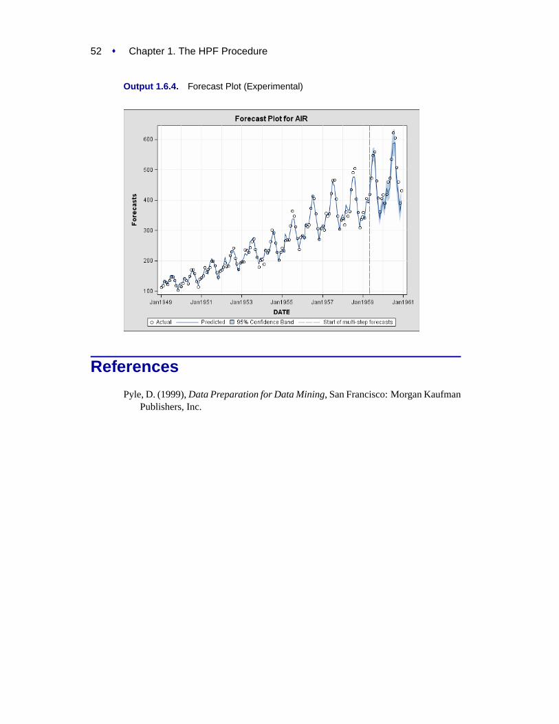
52 � Chapter 1. The HPF Procedure
Output 1.6.4. Forecast Plot (Experimental)
References
Pyle, D. (1999),Data Preparation for Data Mining, San Francisco: Morgan KaufmanPublishers, Inc.