chapter 1 carbon cycle modelling - carnegie ecology€¦ · · 2016-12-22chapter 1 carbon cycle...

CHAPTER 1

Carbon Cycle Modelling

Conference synthesis prepared by:BERT BOLIN, ANDERS BJORKSTROM

CHARLES D KEELING, ROBERT BACASTOW

ULI SIEGENTHALER

1.1. INTRODUCTION

A comprehensive review of the global carbon cycle was given in SCOPE Report 13(Bolin et aI., 1979). In the introductory chapter of that report a comparison was madeof different models of the carbon cycle as well as the modelling assumptions whichcharacterize such models. It is clear that we as yet understand only the broad outline

0[. the carbon cycle.The purpose of the present SCOPE report is not to repeat SCOPE 13 or other sur-

veys of the carbon cycle, but rather to present in a systematic manner basic facts andmodelling considerations that should be further analyzed and possibly included inmore advanced models of the carbon cycle. Hopefully a common base in this waycan be provided, which should aid in the rapidly increasing world-effort to under-stand the global carbon cycle and thereby also the way man may modify it in thefuture.

The increase of the amount of carbon dioxide in the atmosphere since 1957 is

quite accurately known (see chapter 4). Also the emissions of carbon dioxide to theatmosphere due to fossil fuel combustion can be assessed with adequate accuracy(Keeling, 1973 a; Rotty, see chapter 4). In addition, however, man has probablyadded considerable amounts of carbon dioxide to the atmosphere by reducing theextension of the world forests and increasing cultivation of land whereby the oxida-

tion of organic compounds in the soil has been enhanced. The estimates range from1 . 1015g yr-I (Bolin, 1977) to 8 . 1015g yr-I or even more (Woodwell et al., 1978).Oeschger et al. (1980) on the other hand have estimated with the aid of a simplemodel of the oceans that the net carbon flux from terrestrial biota and the soils to the

atmosphere at present probably is at most 10% of the fossil fuel input rate, i.e. merely0.6 . 1015g yr -1. Possibly more effective photoassimilation in some parts ofthe terres-

1

2Carbon Cycle Modelling

trial biosphere may have compensated for the release to the atmosphere due to defo-

restation and increasing cultivation. More detailed models of both the terrestrialbiota and the oceans will be required to resolve this problem.

Because of uncertainties in historical trends, it has not yet been possible to validate

adequately any of the different models of the carbon cycle so far proposed except inbroad outline. Forecasts of the most likely future changes of the atmospheric CO2concentrations are uncertain for this reason in addition to the difficulty in estimatingthe future rates offossil fuel conbustion. It seems likely, however, that an extrapola-tion assuming the increase to be about 50% of the fossil fuel emissions, may yield areasonably good prediction for the next decade or two. Beyond the turn of the cen-tury predictions become increasingly uncertain. Those published so far vary betweena maximum increase of about four-fold (Revelle and Munk, 1977) and eight-fold(Keeling and Bacastow, 1977), if the emissions were eight times the preindustrialamount. Another prediction yields an eight to nine times maximum increase inatmospheric CO2 for an emision of 11.5 times the preindustrial atmospheric amount(Siegenthaler and Oeschger, 1978).

In view of the complex character of the carbon cycle and the necessity to use allrelevant data to ascertain the best possible prediction, the development of moreadvanced models is essential. In order to permit an appropriate use of relevant datamodels need to incorporate sufficient details of the carbon cycle that they can beadequately validated. On the other hand the development of more complex modelsmust be done with care in order that they do not introduce greater uncertainty in theresults because of insufficient data for calibration.

In order to develop more comprehensive and detailed models of the carbon cycle,it is first of all essential to undertake a detailed comparison of present models, toestablish a common data set for validation, and to determine uncertainties byappro-priate sensitivity analyses. These were the main aims of the workshop held at ScrippsInstitute of Oceanography, University of California, La Jolla, California 19-23March, 1979. The first chapter of this report summarizes the outcome in terms of

these aims. It discusses the principal problems of model development and validation,gives a review of the most relevant physical, chemical and biological processes to beincorporated into the next generation of models, and summarizes some importantfeatures of the real carbon cycle that such models should be capable of reproducing.The second chapter presents a more detailed comparison of four simple models ofthe carbon cycle. Recommendations for notations and some technical proceduresare given in chapter 3. Various data sets for validation of carbon cycle models are pro-posed in chapter 4. The remainder of the report contains individual contributions byworkshop participants.

Carbon cycle modelling 3

1.2.SOME PRINCIPAL PROBLEMS OF MODEL DEVELOPMENTAND VALIDATION

1.2.1Degree of simplification

When discussing models of the carbon cycle one needs clearly to specify whatphenomena the model is expected to simulate. Concerned with the atmosphericCO2increase, the principal aim is to predict global averageCO2levelson time scalesfrom about ten to severalhundred years. To accomplish this task, a model must cor-rectly reproduce the carbon fluxes between the atmosphere and the other reservoirson these time scales,but it need for example perhaps not necessarily include detailsof the deep ocean circulation. If we wish to study possible changes over the lastthousand years, the whole of the oceans, the terrestrial biota and the soilsneed to bedealt with adequately. Extending our interest to include changes sincethe 1astglacia-tion means also consideration of the interplay between the oceans and the sedi-ments. The time range in which we are interested clearly influences the degree ofcomplexity of the model.

The development of models of the carbon cycle began with simple three-boxmodels, in which the atmosphere was assumed to be one well-mixedreservoir andthe oceans were described by a surface layer and a deep sea reservoir, both con-sidered as wellmixed (Craig, 1957;Revelle and Suess, 1957;Bolin and Eriksson,1959).Keeling (1973b) discussed this type of model in detail pointing out that theterm ''well-mixedbox" is misleading, since actually the box approach only assumesthat the outgoing fluxes are proportional to the average concentration in the box,which can be realized by reservoirs which are not at all well-mixed.

Later, Oeschger et al. (1975) considered the deep sea as a reservoir in whichexchange is accomplished by vertical eddy diffusion(box diffusion or "BD" model).Obviously a two-box ocean model simplyestablishes general boundary conditions,while the box diffusion model can be regarded as the simplest attempt to reproducethe continuous character of ocean mixing. With respect to atmospheric concentra-tions, the two types of models can be made to respond to an increasing amount ofcarbon dioxide in an almost identical fashion by a proper choice of parameters, asshown in chapter 2.Both types of models are gross simplificationsof the real ocean,and it isnot self-evidentin which wayexperimental data should be best used to deter-mine the parameters. In spite of their limitations, they are of considerable value foranalyzing the principal role of the oceans in the carbon cycle and their response toemissions of carbon dioxide to the atmosphere by man.

During the past decade many studies have been presented, in which also the ter-restrial biota and the soils have been included in a simple manner (Machta, 1972;Keeling 1973b; Revelle and Munk, 1977;Siegenthaler et al. 1978;Bj6rkstr6m, 1979).These models only in a very approximate way depict the principal characteristics ofbiota and soil responses. Stillthey have been useful for obtaining some general fea-tures of the interplaybetween the atmosphere and both the oceans and the terrestrialbiosphere.

4 Carbon Cycle Modelling

Actual physical, chemical and biological processes are described very crudely in

the simple box and box.diffusion models owing to the very few degrees of freedomthat they possess. They are based on empirical relations rather than fIrst principles.Average values over large volumes must be used for the variables chosen, eventhough simple fundamental relations do not directly apply to such average values. Itis difficult to identify data with which to compare model results. Better spatial resolu-tion is therefore necessary when developing more advanced models of the carboncycle (see further section 1.2.3).

The simplest carbon cycle models only describe the circulation and transfer of thevarious carbon isotopes. Many of the processes that need to be considered in realitydepend on or are related to other features of the atmosphere - ocean -land system.

For example the air- sea exchange of carbon dioxide depends on physical-chemicalprocesses right at the surface which are similar to those that determine the exchangeof radon. Radon transfer measurements are therefore of importance for the determi-nation ofthe air- sea exchange of carbon dioxide (see section 1.4.2). The rate of pho-tosynthesis both in the surface layers of the ocean and on land depends on the avail-ability of nutrients and is therefore related to the biogeochemical cycles of particu-larly phosphorus and nitrogen. The ocean circulation plays a similar role for transferof carbon, phosphorus and nitrogen. The ocean circulation in turn is subject todynamic constraints due to the differential heating and rotation of the earth. By con-sidering such more complex interplays other data become useful for calibrating andvalidating the carbon cycle model.

Even though the carbon cycle as a whole needs to be considered in forecasting itsfuture changes, it is convenient fIrst to analyze the more detailed features of theoceans and the terrestrial biosphere separately. To study the sensitivity and responsecharacteristics of the oceans to changes in the atmosphere, we may in an exploratoryphase use a rather simple model of the land biota-soil system. Conversely a two-boxor box diffusion model ofthe oceans may be adequate during the process of develop-ing a more detailed model of the biogeochemical processes on land.

1.2.2Calibration and validation

A model is not to be trusted unless it has been calibrated and validated with realdata. Several problems arise in this context.

Ideally a model should be calibrated as far as possible,by means of independentdata and not by the data which are to be predicted. For example, the parameters of amodel to be used for predicting atmospheric CO2levels should not be determinedfrom the observed CO2increase; rather the comparison between model-calculatedand observed CO2concentration should provide a test validation of the model's pre-dictive capability. Unfortunately, our knowledge about the most important pro-cesses, particularly concerning the terrestrial biota, does not allow a sufficientlyaccurate determination of all the model parameters, and thus it will in general benecessary to make some use of observations of the atmospheric CO2 increase forcalibration.


'Lo~24yrs TO TFigure l: Schematic representation of the age distribution of ocean water since last time at theocean surface, gl(r), and the corresponding age distribution distorted by mixing g2(r), whichtends to establish a maximum value in the vicinity ofthe mean age, ra. The transittime distribu-tion, oCr),is related to gl(r), but cannot be directly deduced from g2(r). Direct observationsduring a period, ro, (e.g. by observations of bomb-produced 14C injections) permits the deter-mination of the value of oCr)for r:;;' ro.

There are in principle two kinds of data that can be used for validation

Data that define the spatial distribution of variables in steady or quasi-steadystate

Data that describe changes that occur as a result of some disturbance of thatstate

It is important to realize that such different data validate different aspects of thebehaviour of the system. The steady state distribution of a tracer in a reservoir (suchas that of pre-bomb 14Cin the sea) is due to the integrated effect of transfer processesduring a period of time that is long compared with the longest transfer time throughthe reservoir (i.e. of the order of 1000 years for 14Cin the sea). We define an agedistri-

bution function g2 (r) as giving the amount of trace material in the reservoir that hasbeen present for a time period longer than r (see Figure 1.1). This function may beuniquely determined if individual molecules can be identified (or individuals in apopulation distribution), but if this is not possible as for example due to mixing in thesea, the observed age distribution is a distorted one as compared with the true one.We can also define a transit time distribution function 15(r) as the amount of tracematerial in the reservoir that has spent a time longer than r, when leaving the reser-

ii


voir. This latter function can be established by observing the flux into (or out from)

the reservoir owing to a tracer disturbance (e.g. bomb-produced 14C,which hasbeentransferred into the sea since about 1956), but only for times less or equal to the timeperiod for which observations are available (e.g. at present about 24 years for bomb14C). Obviously the transit time distribution function is of decisive importance fordeducing the sink characteristics of a reservoir subject to an external disturbancesuch as the oceans when acting as a sink for fossil fuel carbon or bomb-produced 14C.To be able to forecast the future behaviour ofthe carbon cycle we need, however, thetransit time distribution function for a time period as long as the forecast period,which is not directly available from transient 14C data.

If the transfer processes in the reservoir (e.g. the sea) are at steady state, the twofundamental distribution functions just defined are uniquely related (Bolin andRodhe, 1973). The transit time distribution could therefore be derived ifthe age dis-tribution were known. Because of mixing, however, each water parcel that can beidentified contains water of different ages. The observed age distribution of 14Cin thesea therefore cannot be directly used, even though the mean age for the whole oceanis not influenced by mixing. With the aid of a model of the circulation and mixing inthe reservoir, validated with available data, the transit time distribution can be appro-ximately deduced although not directly observed.

1.2.3 Sensitivity analysis

Any model is based on a number of explicit and implicit assumptions and there-fore there are uncertainties in the way reality is being described. It then becomesimportant that rather than merely presenting one most probable description of thecarbon cycle, the range of uncertainty be given, particularly the uncertainty of theresponse to a given emission (as a function of time) of fossil carbon into the atmos-phere. There are many reasons for such uncertainties and these should be carefullyanalyzed separately.

ii

Resolution. Present models of the carbon cycle are mostly very simple, oftenconsist of merely a few reservoirs and have in no case more than about 20degrees of freedom (Bj6rkstr6m, 1979).Obviously reality can only be de-scribed very crudely in this way. To get an idea of how well a given modeldepicts reality we need to increase the resolution. If the higher-resolutionmodel has been validated with real data, one can determine in which regardand to what an extent a simple model can describe the behaviour of a morecomplex model. Few attempts of this kind have been made.

Choiceof modelparameters.The differential equations that typicallydescribethe transient physicaland chemical processes ofthe carbon cycle can often bederived from fundamental equations that govern the system such as the con-tinuity equation, the equation of motion and the laws of thermodynamics.Their application to the particular model usually means a fmite difference for-mulation (Keeling and Bolin, 1967,1968),the accuracy of which depends on


iii

the resolution chosen. On the other hand many processes that need to be de-scribed are theoretically poorly known and are then approximated by empiri-cal relations, usually in terms of rate coefficients.Furthermore these usuallyhave been obtained from observations over a limited range of variation of thevariables concerned. Some problems of the future behaviour of the carboncycle concern rather extreme conditions such as for example an eight-foldincrease of the amount of carbon dioxide in the atmosphere. It is often notknown how well empirical relations hold under such circumstances. Anymodel should be run with extreme choices of empirical parameters to assessthe sensitivity of the results to such uncertainties.

Assumptions of steady-stateor quasi-steadystate. Due to inadequate know-ledge of the present state of the carbon cycle it has become common toassume that a steady-state condition prevailedbefore any essential man-madeemissions of carbon dioxide occurred i.e. before about 1860.Recent researchsuggests,however, that man's influence may have been significanteven earli-er. Furthermore it is possible that climatic variations, such as the Little IceAge, 300-400 years ago, significantlyinfluenced the carbon cycle in earliercenturies. The preindustrial distribution of 14Cin the deep sea may thereforenot have been a steady state distribution. Also natural production of 14Cisknown to varyover time scalesof decades and centuries which interferes withthe assumptions of a steady-state(Suess, 1970,Stuiver, 1980a).An assessmentofthe sensitivityof the model to such assumptions can be made byvaryingtheinitialconditions to see in which way,and how rapidly,an adjustment towardsa steady-statetakes place.Until now we have not been able to derivethe extentto which man has influenced the carbon cyclein the past It appears thereforedesirable to test the model responses to various reasonable assumptions ofwhat these influences may have been.

iv Uncertaintyof datafor validation.In most cases the errors of the measure-ments are wellknown and it is a straightforwardprocedure to analyze the sen-sitivityof the model to such errors. More important, however, is to considercarefullyhow representative the data may be for the particularmodel formula-tion. As already pointed out under (i)above this is closelyassociatedwith theresolution adopted. It may be possible to assess the representativeness of thedata from their variance within the domains dermed by the resolution of themodel. The uncertainty of the model, which is introduced by such lack ofrepresentativeness can then be deduced by a series of sensitivity tests.


1.3.MODELLING ATMOSPHERIC PROCESSES

1.3.1CO2 concentration,BC/I2C, 14C/C

No reliablemeasurements of the CO2concentration in free air are availablebefore1955.Callendar (1958)and Bray (1959)checked the existing measurements, from1857to the early 1950's,Callendar considered numerous data series and selectedthose that appeared most reliable, as to measurement techniques and representa-tiveness for the non-polluted atmosphere. He proposed a "preferred" value of 290ppm for 1870-1900, with a probable accuracy of 1%and could not find any signifi-cant trend during this period.Braymade a statisticalanalysisand obtained by meansof two different weighting schemes mean values for the period 1881-1957 of 294ppm and 311 ppm; most probably the latter is too high. The early measurementsscatter in a relativelywide range. Most authors working on the CO2problem haveassumed 19th century concentrations of approximately 290 ppm, which value pro-bably has an uncertainty of:t 10ppm. Since 1958,continuous measurements havebeen made by Keeling and his co-workersat Mauna Loa, Hawaii, and at the SouthPole. Flight data for the period 1962-1979 from the north polar regions have beencollected by Bischof(1977).Summaries of these and other relevant data are given inchapter 4 of this report.

The pre-industrialatmospheric 14C/Cratio, corrected for isotopic fractionation toa standard value for ol3C of - 25%0 is often assigned the number 100 percentmodem or A14C= 0%0.The defmitions of the different quantities used in 14Cworkand the details for the I3Ccorrection are described by Stuiver and Polach (1977)andsummarized in Chapter 3.Even before man disturbed the natural14Cdistribution byfossil fuel CO2and bomb-14C,the atmospheric 14C/Cratio varied, showing short-term (about hundred years) ''wiggles''and long term (several thousand years) varia-tions (Suess, 1970).While fluctuations of the 14Cproduction rate probablyhave beena dominant cause of the 14Cvariations,changes in the exchange pattern of the globalcarbon systems,for instance due to climatic changes probably also have affected theatmospheric 14Cconcentration (cfSiegenthaler et aI., 1980,and Bolin, this volume).As noted earlier there wasthus probably never a perfect steady state.Exchange ratesas deduced from a presumed steady state distribution may therefore be incorrect.

From the middle oflast century until 1954the 14C/Cratio of atmospheric CO2haddecreased by 2.0to 2.5%primarilydue to the emission of 14C-freeCO2by fossilfuelcombustion (Suess, 1965,Lerman et al., 1970).This estimate is based on measure-ments of the 14Ccontent of dendro-chronologicallydated tree rings.Since 1954thisgradual decrease has been completely overshadowed by the rapid increase due tonuclear bomb testing. These changes have been recorded by direct measurementsduring the last 25years (Nydal, 1978;see chapter 4 of this volume). They are usefulfor calibration or validation of carbon cycle models (cf Keeling, 1973b).

The mean I3C/12Cratio of atmospheric CO2 expressed as ol3C is about -7%0.The preindustrial value is uncertain since no direct measurements are available.


Measurements by Keeling et al. (1979)show that it has decreased from -6.7%0 in1956to -7.3%0 in 1978.This is considerably less than would be expected ifthis wasdue solely to dilution caused by emission of fossil CO2with a characteristic ol3C-value of about - 27%0.The observed decrease is smaller because atmospheric CO2exchanges with the other carbon reservoirs.A closer analysisis criticallydependenton the isotopic fractionation at the air-ocean boundary. Model calculations bySiegenthaler et al. (1978) predict a shift of -0.7%0 from 1860to 1970 assumingconstant biomass. Keeling et al. (1980)conclude that the measurements hardly aresensitive enough to distinguishbetween oceanic and biospheric uptake of industrialCO2. Nevertheless ol3C measurements may well provide useful information formodel validation if pursued to 1990or longer.

Since carbon in wood is assimilated from atmospheric CO2 a record of thedecrease of ol3C in the atmosphere is stored in tree rings.Measurements of ol3Cintree rings (Stuiver, 1978;Freyer, 1979)show a decrease of 1-2%0 between about1860and 1970.The interpretation of the tree-ring data is, however, not straightfor-ward. ol3Ctime series measured in different trees often deviatemuch from one ano-ther. Tans (1978)found that ol3Cwithin one single tree-ring can vary by severalpermil in different circumferential directions. The largest intra-ringvariation was4.9%0.Tans further found that ol3Cvariationsin tree-ringsare correlated with temperatureand yearly total precipitation; other authors also report a correlation withtemperature (Pearman et aI.,1976;Wilson and Grinsted, 1977).Furthermore, youngtrees standing in a forest environment assimilate respiratoryCO2with low ol3Ccon-centration (Freyer, 1979).Other factors, e.g. physiological,probably also influenceol3C of tree-ring carbon. Therefore, ol3C values deduced from tree rings do notnecessarily show the actual ol3C variations of atmospheric CO2and must be usedwith care for calibration and validation of carbon cycle models.

1.3.2Atmosphericmixing

The time scale for mixing between the two hemispheres is 0.6 to 2 years (Bolin andKeeling, 1963;Junge and Czeplak, 1968)and the mean residence time of air in thestratosphere, defined 'as the ratio of stratospheric mass to the mean air exchangeacross the tropopause, has been determined as 1.0 to 1.5years (Krey et aI., 1974;Reiter, 1975),while the exchange time between the upper stratosphere and the tro-posphere is longer as deduced from changes of 14Cfollowingthe nuclear tests 1958-1962(cf Machta, 1972),but the mass involved is small.

There are quite marked seasonal CO2 variations, with peak-to-peak amplitudesranging from 1ppm at the South Pole to about 15ppm in high Northern Latitudes.There have been several attempts to analyse the seasonal variations in terms ofsources and sinks and of atmospheric mixing (Bolin and Keeling, 1963,Junge andCzeplak, 1968,Machta, 1973,Pearman, 1980).Machta (1973)calculated the atmo-spheric CO2 variations by means of a 2-dimensional diffusion model of the atmo-sphere, using an estimated function for the biospheric CO2sources and sinks,which


ATMOSPHERE

No = (615:!:20)'101~gC""(290:!:10)ppm613C= -6%0~ll.C=.:!:O%o

TERRESTRIALBIOTA

Na=(800:!:100)'1015gCh'3C=-25 %0b,14C= 0 %0

OCEAN

~j~~Q.J9~!: _l~7.~mJDIC:Nm=670'10' gCDI'4C: b,14C=-(50:!:10)%0

HUMUS,SOIL

Organic C:(1500:t200)'10'5g Cb'3C=-25%0

~4C= -(50:t 50) %0TOTALSEA

DIC: 37.1,00'10'5gC

D113C:cS13C=O%o

D114C:84C=-(160:t20)%0

Organic C: ,.. 1000 .10159 C

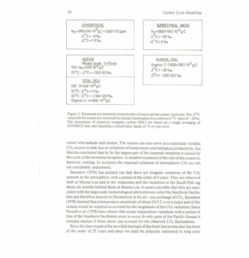
Figure 2: Estimated pre-industrial characteristics of major global carbon reservoirs. The A14Cvalues forthe oceans are corrected for isotope fractionation to a common 0 l3C value of - 25%0.The inventories of dissolved inorganic carbon (DIC) are based on a rough averaging ofGEOSECS data and assuming a mixed layer depth of 75 m (see text).

varied with latitude and season. The oceans can also serve as a seasonally variableCO2 source or sink due to variations of temperature and biological productivity, butMachta concluded that by far the largest part of the seasonal variations is caused bythe cycle of the terrestrial biosphere. A detailed treatment of the role of the oceans is,however, missing. In summary the seasonal variations of atmospheric CO2 are notyet completely understood.

Bacastow (1976) has pointed out that there are irregular variations of the CO2amount in the atmosphere, with a period of the order of 4 years. They are observedboth at Mauna Loa and in the Antarctica and the variations at the South Pole lagabout six months behind those at Mauna Loa. It seems plausible that they are asso-ciated with the large-scale meteorological phenomenon called the Southern Oscilla-tion and therefore depend on fluctuations in the air-sea exchange of CO2. Bacastow(1978) showed that a temperature amplitude of about :to.5 C over a major part of theoceans would be required to account for the magnitude of the CO2 variations. SinceNewell et al. (1978) have shown that ocean temperature variations with a period ofthat of the Southern Oscillation seem to occur in only parts of the Pacific Oceans itremains unclear if these alone can account for the observed CO2 fluctuations.

Since the time required for an e-fold increase ofthe fossil fuel production has beenof the order of 25 years and since we shall be primarily interested in long term


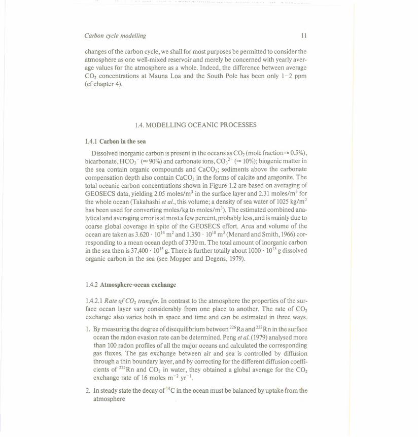
changes of the carbon cycle,we shall for most purposes be permitted to consider theatmosphere as one well-mixedreservoir and merely be concerned with yearlyaver-age values for the atmosphere as a whole. Indeed, the difference between averageCO2 concentrations at Mauna Loa and the South Pole has been only 1-2 ppm(cf chapter 4).

1.4.MODELLING OCEANIC PROCESSES

1.4.1 Carbon in the sea

Dissolved inorganiccarbon is present in the oceans as CO2(mole fraction ~ 0.5%),bicarbonate, RC03 - (~90%) and carbonate ions,CO/- (~ 10%);biogenicmatter inthe sea contain organic compounds and CaC03; sediments above the carbonatecompensation depth also contain CaC03 in the forms of calcite and aragonite. Thetotal oceanic carbon concentrations shown in Figure 1.2are based on averaging ofGEOSECS data, yielding2.05moles/m3 in the surface layer and 2.31moles/m3 forthe whole ocean (Takahashi et af., this volume; a density of sea water of 1025kg/m3has been used for converting moles/kg to moles/m3). The estimated combined ana-lyticaland averagingerror isat most a fewpercent, probablyless,and ismainly due tocoarse global coverage in spite of the GEOSECS effort. Area and volume of theocean are taken as 3.620. 1014m2and 1.350. 1018m3(Menard and Smith, 1966)cor-responding to a mean ocean depth of 3730m. The total amount of inorganic carbonin the sea then is 37,400. 1015g.There isfurther totallyabout 1000. 1015g dissolvedorganic carbon in the sea (see Mopper and Degens, 1979).

1.4.2 Atmosphere-ocean exchange

1.4.2.1 Rate of CO2 transfer. In contrast to the atmosphere the properties of the sur-face ocean layer vary considerably from one place to another. The rate of CO2exchange also varies both in space and time and can be estimated in three ways.

1. By measuring the degree of disequilibrium between 226Raand 222Rnin the surfaceocean the radon evasion rate can be determined. Peng et af. (1979) analysed morethan 100 radon profiles of all the major oceans and calculated the correspondinggas fluxes. The gas exchange between air and sea is controlled by diffusionthrough a thin boundary layer, and by correcting for the different diffusion coeffi-cients of 222Rn and CO2 in water, they obtained a global average for the CO2exchange rate of 16 moles m-2 yr-I.

2. In steady state the decay of 14Cin the ocean must be balanced by uptake from theatmosphere


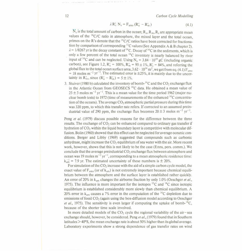
AR~ Ns = Farno(R~ - R:r,) (4.1)

Ns is the total amount of carbon in the ocean; Ra, Rrn,Rs are appropriate meanvalues of the 14C/C ratio in atmosphere, the mixed layer and the total ocean,primes on the R's denote that the 14C/C ratios have been corrected for fractiona-

tion by comparison of corresponding BC values (See Appendix A & B chapter 2).A = 1/8267 yr is the decay constant of 14C.Decay of 14Cin the sediments, which isonly a few percent of the total ocean 14Cinventory is nearly balanced by riverinput of 14Cand can be neglected. Using Ns = 3.84 . 1019gC (including organiccarbon), see Figure 1.2, R~ = 100%, R:n = 95 i:: 1%, R~ = 84%, and referring the

global flux to the to~l ocean surface area, 3.62 . 1014m2, we get from eq. (4.1) F arno= 18moles m-2 yr- . The estimated error is :t25%, it is mainly due to the uncer-tainty in R:n, since (R~ - R:n) = 5:t 1%.

3. Stuiver(1980b) calculated the inventoryofbomb-14Cand the CO2exchange fluxin the Atlantic Ocean from GEOSECS 14Cdata. He obtained a mean value of23:t 3 moles m-2 yr-l. This is a mean value for the time period 1962(major nu-clear bomb tests) to 1972(time of measurements of the enhanced 14Cconcentra-tion of the oceans).The averageCO2atmosphericpartialpressure during this timewas 320 ppm, to which this transfer rate refers. If corrected to an assumed prein-dustrial value of 290 ppm, the exchange flux becomes 20:t 3 moles m-2 yr-l.

Peng et al. (1979) discuss possible reasons for the difference between the threeresults. The exchange of CO2can be enhanced compared to ordinary gas transfer ifhydration of CO2within the liquid boundary layer is competitive with molecular dif-fusion. Bolin(1960)showed that this effect can be neglected for averageoceanic con-ditions. Berger and Libby (1969) suggested that compounds such as carbonicanhydrase, might increase the CO2equilibrium of sea water withthe air.More recentwork, however, shows that this is not likely to be the case (Enos, pers. comm.). Weconclude that the averagepreindustrial CO2exchange flux between atmosphere andocean was 19moles m-2 yr-l, corresponding to a mean atmospheric residence time:k~ = 7.9 yr. The estimated uncertainty of these numbers is :t 20%.

For simulationof the CO2increase withthe aidof a simplecarbon cyclemodel, theexactvalueof Farno(orof karn)isnot extremelyimportantbecausechemicalequili-brium between the atmosphere and the surface layer is established rather quickly.An error of 20%in karnchanges the airborne fraction by only 1.0%(Oeschger et al.,1975).The influence is more important for the isotopes BC and 14Csince isotopicequilibrium is established considerably more slowlythan chemical equilibrium. A20%error in karncauses a 7%error in the computation of the 14Cdepletion due toemissions offossil CO2(again using the box-diffusionmodel according to Oeschgeret al., 1975).The sensitivity is even larger if computing the uptake of bomb-14C,because of the shorter time scale involved.

In more detailed models of the CO2 cycle the regional variabilityof the air- seaexchange should, however, be considered. Peng et at., (1979)found that in Southernlatitudes> 4O"S,the mean exchange rate is about 50%higher than itsglobal average.Laboratory experiments show a strong dependence of gas transfer rates on wind


velocity (e.g. liihne et al., 1979). The observed regional differences may therefore bedue to latitudinal variations of wind velocities. The importance of such differencesfor the global CO2 transfer between the atmosphere and the sea has not yet been pro-perly accounted for in the carbon cycle models developed so far.

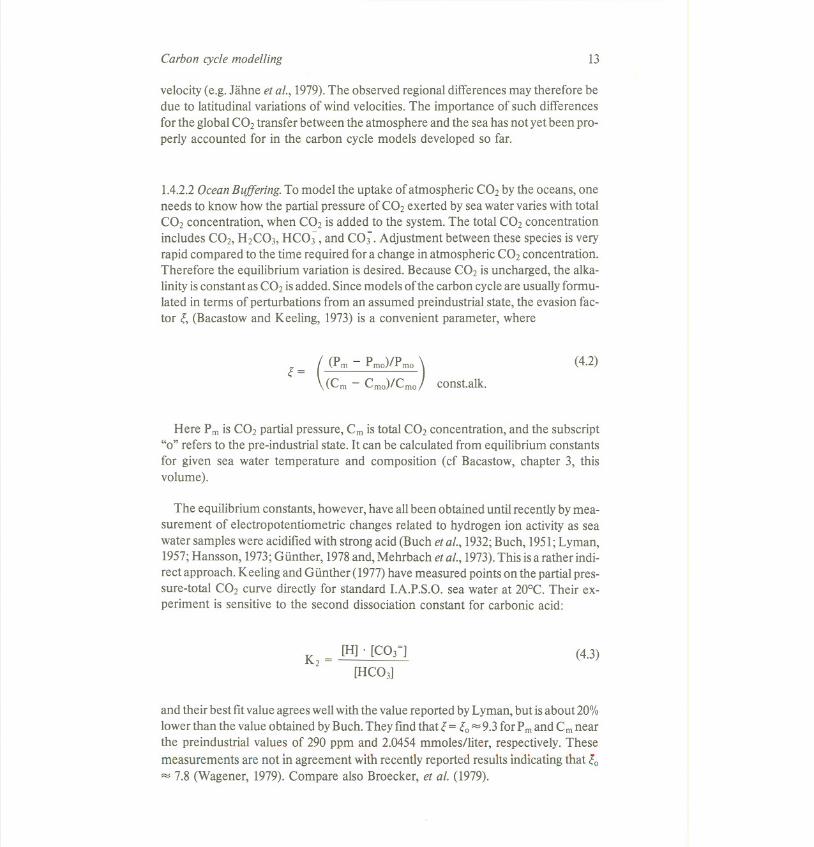
1.4.2.2 Ocean Buffering. To model the uptake of atmospheric CO2 by the oceans, oneneeds to know how the partial pressure of CO2 exerted by sea water varies with totalCO2 concentration, when CO2 is added to the system. The total CO2 concentrationincludes CO2, H2C03, HCO;, and CO;. Adjustment between these species is veryrapid compared to the time required for a change in atmospheric CO2 concentration.Therefore the equilibrium variation is desired. Because CO2 is uncharged, the alka-linity is constant as CO2 is added. Since models ofthe carbon cycle are usually formu-lated in terms of perturbations from an assumed preindustrial state, the evasion fac-tor 1;,(Bacastow and Keeling, 1973) is a convenient parameter, where

((Pm - Pmo)/Pmo

)1;=(Cm - Cmo)/Cmo const.alk.

(4.2)

Here Pm is CO2 partial pressure, Cm is total CO2 concentration, and the subscript"0" refers to the pre-industrial state. It can be calculated from equilibrium constantsfor given sea water temperature and composition (cf Bacastow, chapter 3, thisvolume).

The equilibrium constants, however, have all been obtained until recently by mea-surement of electropotentiometric changes related to hydrogen ion activity as sea

water samples were acidified with strong acid (Buch et aI., 1932;Buch, 1951; Lyman,1957; Hansson, 1973; Gunther, 1978 and, Mehrbach et al., 1973). This is a rather indi-rect approach. Keeling and Gunther (1977) have measured points on the partial pres-sure-total CO2 curve directly for standard I.A.P.S.O. sea water at 20DC. Their ex-periment is sensitive to the second dissociation constant for carbonic acid:

[H] . [CO ~]K2 = 3

[HC03]

(4.3)

and their best fit value agrees well with the value reported by Lyman, but is about 20%lower than the value obtained by Buch. They find that 1;= 1;0"'"9.3 for Pmand Cm nearthe preindustrial values of 290 ppm and 2.0454 mmoles/liter, respectively. These

measurements are not in agreement with recently reported results indicating that (0

"'" 7.8 (Wagener, 1979).Compare also Broecker, et al. (1979).


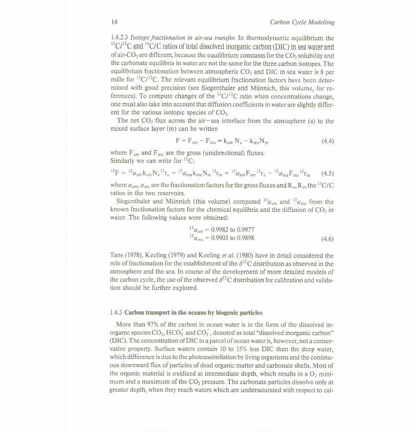
1.4.2.3Isotopefractionation in air-seatransfer.In thermodynamic equilibrium the13CfI2Cand 14CfCratios oftotaldissolvedinorganiccarbon(DIC)in seawaterandof air-CO2are different,because the equilibrium constants for the CO2solubilityandthe carbonate equilibria in water are not the same for the three carbon isotopes.Theequilibrium fractionation between atmospheric CO2and DIC in sea water is 8 permille for 13CfI2C.The relevant equilibrium fractionation factors have been deter-mined with good precision (see Siegenthaler and Miinnich, this volume, for re-ferences). To compute changes of the 13CfI2Cratio when concentrations change,one must also take into account that diffusioncoefficientsin water are slightlydiffer-ent for the various isotopic species of CO2.

The net CO2 flux across the air-sea interface from the atmosphere (a) to themixed surface layer (m) can be written

F = Fam - Fma = kamNa - kmaNm (4.4)

where F amand F maare the gross (unidirectional) fluxes.Similarly we can write for 13C:

13F = 13aamkamNa 13ra - 13amakmaNm 13rm - 13aamFam 13ra - 13amaFma 13rm (4.5)

where aam,amaare the fractionation factors for the grossfluxes and Ra,Rmthe 13CfCratios in the two reservoirs.

Siegenthaler and Miinnich (this volume) computed 13aamand 13amafrom theknown fractionation factors for the chemical equilibria and the diffusion of CO2inwater. The following values were obtained:

13aam = 0.9982 to 0.9977

13ama = 0.9903 to 0.9898 (4.6)

Tans (1978),Keeling (1979)and Keeling et at. (1980)have in detail considered therole of fractionation for the establishment ofthe 613Cdistribution as observed in theatmosphere and the sea. In course of the development of more detailed models ofthe carbon cycle,the use of the observed 613C distribution for calibration and valida-tion should be further explored.

1.4.3 Carbon transport in the oceans by biogenic particles

More than 97% of the carbon in ocean water is in the form of the dissolved in-

organic species CO2, HCO; and CO;, denoted as total "dissolved inorganic carbon"(DIe). The concentration ofDIC in a parcel of ocean water is, however, not a conser-vative property. Surface waters contain 10 to 15% less DIC than the deep water,which difference is due to the photoassimilation by living organisms and the continu-ous downward flux of particles of dead organic matter and carbonate shells. Most of

the organic material is oxidized at intermediate depth, which results in a O2 mini-mum and a maximum of the CO2 pressure. The carbonate particles dissolve only atgreater depth, when they reach waters which are undersaturated with respect to cal-


cium carbonate. Their dissolution affects DIC and alkalinity, but not the oxygen con-centration. The transport of carbon by the particle flux is 10 to 15 percent ofthe totalvertical flux of carbon. In a steady state, as is commonly assumed to have prevailedduring preindustrial time, this downward flux by biogenic particles, detritus, isbalanced by an upward flux due to water motions as described in the next section.

The marine biological productivity in the surface waters is primarily controlled bythe availability of nutrients, particularly nitrogen and phosphorus, and is probablynot influenced by changes in DIC. For this reason biogenic particle flux is often notincluded in models used for simulating the response of the oceans to increasinganthropogenic CO2 emissions. Ifwe are only interested in such perturbations of thesystem, we may deduce the appropriate perturbation equations from the completemodel equations. They are obtained as the difference between the equations for thetime varying concentrations and those valid for the steady state. Terms that describeprocesses which do not change due to the increased amount of CO2 in the atmo-sphere and the oceans then disappear.

1.4.4 Oceanic circulation

Complete mixing of a tracer in the ocean is a process that requires many centuries.On the other hand, vast sub-volumes of the ocean exist, within which the mixing ismuch more rapid. When we wish to analyze the characteristics ofthe world ocean as

a sink for fossil fuel CO2, we must therefore carefully consider how to subdivide theocean to account adequately for such differences. When modelling the ocean inglobal carbon cycle studies, horizontal homogeneity has almost always beenassumed. We therefore begin with a description of the ocean and its circulation thatparticularly emphasizes the variations in the vertical, but will fmd that further detailsneed to be considered to describe the ocean circulation adequately in carbon cycle

modelling.

1.4.4.1Themixed layer.The uppermost few tens of meters of the ocean, the so calledmixed layeror surface layer,are rapidlymixed in the verticalbywindaction. The dis-tribution of radon reveals that mixing takes place within a few days (Broecker andPeng, 1974).This is short in comparison to the time scales involved in the seculartrend of carbon dioxide, so that the mixed layer can safelybe regarded as verticallywell mixed. The depth hmof the mixed layervaries between about 20m and 200m;at high latitudes a mixed layer depth cannot be clearly defined because verticalgradients are weak. An extended investigationbyBathen (1972)in the North Pacific,using bathythermograph observations, yielded a seasonallyand regionallyaveragedvalue of75 m for hm.With a depth of75 m, the mixed layercontains about 10%morecarbon (in the form of CO2(gas), HCOj, and cOj-) than the atmosphere (in theform of CO2).The carbon in the mixed layerconstitutes about 2%of the total carboncontent in the ocean.


In some two-boxmodel studies, the mixed layer depth hmhas been treated as anadjustable parameter, and values of up to several hundred meters have been used(Keeling, 1973b;chapter 2, this volume). The motivation for these experiments isthat it is not unreasonable to include part of the main thermocline into an extendedmixed layer.Nevertheless, an adjustable model mixed layer should be clearlydistin-guished from the oceanographically defined mixed layer. It is desirable rather toaccount for the mixing processes into the thermocline region explicitly in order toaccount properly for the transfer of carbon dioxide to deeper layersof the ocean (seefurther below).

The solubilityof CO2in seawater varieswithtemperature. This fact causes a trans-fer of CO2in the atmosphere from warm regions, where the solubility in the surfacewaters is comparatively low, to polar regions with high CO2solubilityin the surfacewaters (Bolin and Keeling, 1963).A net transfer from high to low latitudes in theoceans must occur to balance the atmospheric flux. Keeling and Bolin (1968)accounted for this in a three-box model and this fact has also been considered byBjorkstrom (1979).As willbe seen below a distinction between cold and warm sur-face water seems necessary for other reasons to describeproperly the carbon transferin the oceans. The differences in solubility should then also be accounted for.

1.4.4.2 The main oceanic thermocline (intermediate water). The mixed layer at thewarm ocean surface is separated from the cold deep waters by a transition zone, themain thermocline. This zone is next to the mixed layer, of main importance for theuptake of anthropogenic CO2. The simplest way to take into account the continuouscharacter of oceanic mixing into the thermocline region (and the deep sea) is to con-sider it as a diffusion process of Fickian type, in which the fluxes are proportional toconcentration gradients. The concept of eddy diffusion is used by several authors todescribe vertical profiles below 1 km depth (see below), and Oeschger et at. (1975)used it in their box diffusion (BD) model for describing the vertical transfer from thesurface into the thermocline and the deep sea, assuming a constant eddy diffusivityK. The essential difference between the two-box (2B) approach (see 1.4.4.3) and thebox diffusion approach is not so much the discrete or continuous character ofoceanic concentration profiles, but rather a different time dependence of the down-ward flux, as discussed in detail by Oeschger et at. (1975). For a perturbation withcharacteristic time r« 103years, the flux from mixed layer to deep sea is propor-tional to r-1I2for BD, i.e. the flux increases with decreasing r,but is independentofrin the 2B model.

Polewards of the oceanic polar fronts well defined mixed layers usually do notexist throughout the year. The surface water rather mixes rapidly with deeper strata.The thermocline region below the warm surface water at middle and low latitudes ismaintained by rather effective quasi-horizontal exchange with these cold surfacewaters. To account for this Broecker et at. (1971) in their model introduced a directconnection between the atmosphere and the thermocline region which extendsdown towards 1000 m depth. In such a case the role of the intermediate water


depends on its volume and the air-sea transfer in the outcrops in the cold surfacewaters. To a fIrst approximation this model is equivalent to the two-box model(mixed layer-deep sea) assuming a considerably deeper mixed layer (Keeling,1973).A model including a direct outcrop of intermediate water differs,however, inan important way from purely one-dimensional models (as the BD-model), sinceCO2(or other matter) entering the cold ocean surface is diluted into a considerablylarger volume than CO2 entering the warm mixed layer.

Broecker et af. (1978)have deduced interesting features of the thermocline regionmaking use of the penetration of bomb-produced 14C(and tritium) in the Atlantic. Inthe areas of the subtropicalanti-cyclonesthe downwardtransfer of 14Cismuch moremarked than in the zone between 15°Nand 15°S,where an average upwardvelocityof27 m yr-l is deduced. Such regional differences in the verticaltransfer Ofl4C(andpresumably offossil fuelproduced excess CO2)have not been included in any modelof the global carbon cycle.Bj6rkstr6m (1979)has formulated a simple two-reservoirmodel of the intermediate water and emphasizes the importance of its proper con-sideration in the development of a global carbon cyclemodel. This problem willbefurther discussed in section 1.4.4.4.

1.4.4.3Transferinto thedeepsea.The replenishment of water belowthe main oceanicthermocline is driven by a combination of coolingof surface water in high latitudesand a supply of geothermal heat at the ocean floor. The deep water formation isintense around the Antarctic, where ithas been estimated byMunk (1966)to amountto about 30 . 106m3Is. This estimate was based on salinity changes in connectionwith the formation of ice during the winter season. Gordon (1975)estimates the con-vection in the region to amount to 38 . 106m3/s by considering the heat balance.Contributions to the deep water formation also come from the North Atlantic.Recent estimates of the magnitude of these vary between 10 and 30 . 106 m3Is(Broecker, 1979).

It is thus generally accepted that a net flux of water into the deep sea takes place athigh latitudes, which is balanced by a slow upward motion over the rest of the oceans.The total downward flow of 40-60. 106 m3 S-l corresponds to a mean upwardmotion of 4-6 m yr-l and implies a turnover time for the deep water of 1000-600years. The mean age of the deep sea water is close to 1000 years, if taking the average14C/C value of the ocean below the thermocline to be 84% and that of surface water

95% relative to the pre-industrial value for the atmosphere. As has been pointed outpreviously, however, the turnover time (which is equal to the mean transit time) andthe mean age need not be the same.

Let us next consider a vertical column of water in those parts of the ocean, where

slow upwelling occurs. Some diffusive exchange in the vertical also takes place. Thetracer concentration, C, is then governed by the equation


ij2 C {}CK - - w - - ~C-t- J = 0

iJZ2 iJz

(4.7)

where K is the vertical diffusivity (assumed to be constant), w is the vertical upward

velo~ity, Ais the decay constant for the tracer (= 0 for inactive tracers), J denotes thenet of sources and sinks, which include processes associated with decomposition offalling detritus and horizontal exchange with regions of downwelling. With the aid ofeq. (4.7) and proper assumptions about Q and S, we can determine K and w from ver-tical concentration profiles of 14C/C, oxygen and other tracers (Wyrtki, 1962;Munk, 1966; Craig, 1969; Rooth and Ostlund, 1972).

It is important, however, to verify these results in three-dimensional models of theocean circulation (Bryan, 1969; Kuo and Veronis, 1970; Holland, 1971; Veronis,1975). Such computations show that great care must be taken to avoid significanterrors in the semi-empirical approach that has been followed (see Veronis, 1975).Average values forK and wvary considerably: 0.2 cm2 sec-I <K < 1.3 cm2 sec-I and1.4 m yr-I <w < 10 m yr-I. The vertical tracer distributions primarily determine theratio, K/w, which is a characteristic length scale, and small values ofK go with smallvalues of w. The wide range of values shows that computations so far are not con-clusive and particularly the role of slant convection along surfaces of constantdensity seems to be an important mechanism for water exchange in the thermoclineregion that need be carefully considered (cf also Welander, 1971).

In modelling the carbon cycle three different models for exchange between thesurface (mixed) layer and the thermocline region and the deep sea have been ad-vanced. They all are gross simplifications and do not represent more than first ap-proximations to the role of the oceans in the carbon cycle. They are compared morein detail in chapter 2 of this volume. The use of a three-dimensional global model ofthe oceans in dealing with the carbon cycle has not yet been attempted (see furthersection 1.4.5).

1. The ocean is divided into two boxes, a surface mixed layer of depth hm, and thedeep sea (two box, 2B, model). The rate of exchange between the two reservoirs isgiven by the exchange coefficient kdm = Td~,where Tdmis the turnover time of the

deep sea (cf Keeling, 1973 b). Oceanic mixing is thus described by the two para-meters hm and kdm.The depth hm is in general treated as an adjustable parameter;kdmcan be derived from a 14Cbalance of the deep sea, analogously to the calcula-tion ofkam (see 1.4.2.1). Keeling (1973 b) has analyzed this problem and shownthat the value for Tdmobtained without considering the gravitational flux ofdetritus

14R 14R- -I - mo - do

Tdm - kdm - 14A Rdo

is an overestimate by only a few percent in comparison with a computation inwhich detritus flux is properly accounted for and that it exclusivelydepends onthe fractionation of the 14Ccarbon isotope in the photosynthesis being differentfrom unity.

(4.8)


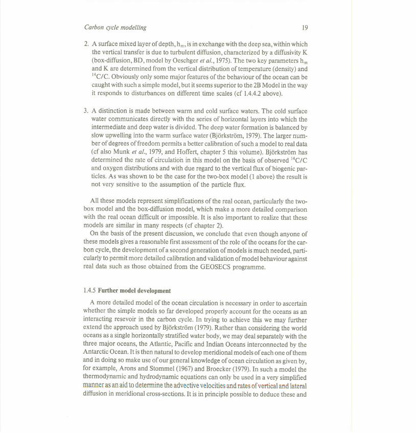
2. A surface mixed layer of depth, hm, is in exchange with the deep sea, within whichthe vertical transfer is due to turbulent diffusion, characterized by a diffusivity K(box-diffusion, BD, model by Oeschger et al., 1975). The two key parameters hmand K are determined from the vertical distribution of temperature (density) and14C/C. Obviously only some major features of the behaviour of the ocean can becaught with such a simple model, but it seems superior to the 2B Model in the wayit responds to disturbances on different time scales (cf 1.4.4.2 above).

3. A distinction is made between warm and cold surface waters. The cold surfacewater communicates directly with the series of horizontal layers into which theintermediate and deep water is divided.The deep water formation is balanced byslow upwelling into the warm surface water (Bjorkstrom, 1979).The larger num-ber of degrees of freedom permits a better calibration of such a model to real data(cf also Munk et al., 1979,and Hoffert, chapter 5 this volume). Bjorkstrom hasdetermined the rate of circulation in this model on the basis of observed 14C/Cand oxygen distributions and with due regard to the vertical flux of biogenic par-ticles. As was shown to be the case for the two-box model (1 above) the result isnot very sensitive to the assumption of the particle flux.

All these models represent simplifications of the real ocean, particularly the two-box model and the box-diffusion model, which make a more detailed comparisonwith the real ocean difficult or impossible. It is also important to realize that thesemodels are similar in many respects (cf chapter 2).

On the basis of the present discussion, we conclude that even though anyone ofthese models gives a reasonable first assessment of the role of the oceans for the car-

bon cycle, the development of a second generation of models is much needed, parti-cularly to permit more detailed calibration and validation of model behaviour againstreal data such as those obtained from the GEOSECS programme.

1.4.5Furthermodeldevelopment

A more detailed model of the ocean circulation is necessary in order to ascertainwhether the simple models so far developed properly account for the oceans as aninteracting resevoir in the carbon cycle. In trying to achieve this we may furtherextend the approach used by Bjorkstrom (1979).Rather than considering the worldoceans as a singlehorizontally stratifiedwater body, we may deal separatelywith thethree major oceans, the Atlantic, Pacific and Indian Oceans interconnected by theAntarctic Ocean. It is then natural to developmeridional models of each one ofthemand in doing so make use of our general knowledgeof ocean circulation as given by,for example, Arons and Stommel (1967)and Broecker (1979).In such a model thethermodynamic and hydrodynamic equations can only be used in a very simplifiedmanner as an aid to determine the advectivevelocitiesand rates ofvertical and lateraldiffusion in meridional cross-sections.It is in principle possible to deduce these and


to estimate other processes such as rates of photoassimilation, detritus fall and decay

if a sufficient number of tracer distributions is available (cf Arons and Stommel,1967; Keeling and Bolin, 1967, 1968).In practice, however, we meet considerable dif-ficulties. The sources and sinks for some tracers are similar, in which case suchdeductions become very sensitive to small errors (the set of simultaneous equationsthat describes the tracer balance is ill-conditioned). Simple test computations alsoshow that the density distribution, i.e. the static stability, needs to be considered care-fully. The approximation of the continuous differential equations, that govern thetracer continuity, by fmite differences on a coarse rectangular grid may well intro-duce unacceptable errors. It is important to distinguish carefully between transferalong surfaces of constant density and in the vertical direction as discussed by We lan-der (1971), Veronis (1975) and Walin (1977). Even though there probably are notenough data to validate such models properly, this kind of model development maystill be useful in trying to assess the most important processes to be considered inmodelling the oceans in more detail.

Another approach may be considered. General circulation models of the oceanshave been developed that describe the three-dimensional motions ofthe sea as deter-mined from external boundary conditions i.e. heating, cooling, amount of precipita-tion and wind stress at the air-sea interphase and geothermal heating and frictionaldrag at the bottom (Bryan, 1969). Starting from an initial state of rest, these modelspredict the fields of temperature, salinity and velocity and, if run for several hundredyears, seek a quasi-equilibrium, that in its gross features resembles the structure andcirculation of the real ocean. Using such a model the equilibrium distribution oftra-cers such as oxygen and 14Ccan be determined (Holland, 1971; Veronis, 1975). As amatter of fact such computations represent an important way of validating the model,if equilibrium distributions are known. The role of the oceans for transfer of carboncan also be simulated in this way and thereby the role ofthe ocean in the carbon cyclebe determined.

1.5.MODELLING THE SOILSAND TERRESTRIAL BIOTA

1.5.1 Key problems

Terrestrial vegetation and dead organic matter in the soil constitute components inthe carbon cycle that are significant as regards size and characteristic time scalescompared to the atmosphere-ocean system (Whittaker and Likens, 1975; ScWesin-ger, 1977, 1979; Bolin et al., 1979). We need therefore consider how we best canmodel the terrestrial processes with our present state of knowledge and include themin a global carbon model. At this time we are particularly hampered by the fact that:

1. the general features of the terrestrial biomes are only known in their broad out-lines, particularly their response to external influences. For example we donot


know well how the global primary production may change due to increasingatmospheric CO2 concentrations.

2. we lack historical series of data on man's impact on the terrestrial biomes as todeforestation, agriculture, afforestation and other direct interferences, expressedas amounts of CO2 emitted to or withdrawn from the atmosphere per year.

1.5.2 The global distribution of terrestrial biota as described by a system of biomes

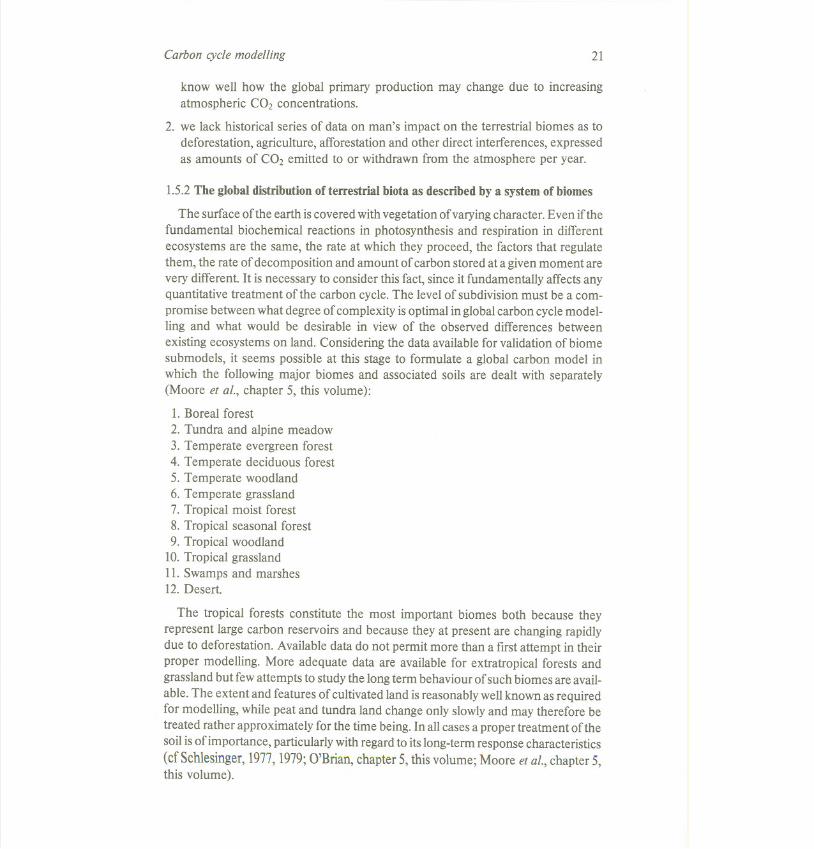
The surface ofthe earth is covered with vegetation of varying character. Even ifthefundamental biochemical reactions in photosynthesis and respiration in differentecosystems are the same, the rate at which they proceed, the factors that regulatethem, the rate of decomposition and amount of carbon stored at a given moment arevery different. It is necessary to consider this fact, since it fundamentally affects anyquantitative treatment of the carbon cycle. The level of subdivision must be a com-promise between what degree of complexity is optimal in global carbon cycle model-ling and what would be desirable in view of the observed differences betweenexisting ecosystems on land. Considering the data available for validation of biomesubmodels, it seems possible at this stage to formulate a global carbon model inwhich the following major biomes and associated soils are dealt with separately(Moore et al., chapter 5, this volume):

1. Boreal forest2. Tundra and alpine meadow3. Temperate evergreen forest4. Temperate deciduous forest5. Temperate woodland6. Temperate grassland7. Tropical moist forest8. Tropical seasonal forest9. Tropical woodland

10. Tropical grassland11. Swamps and marshes12. Desert.

The tropical forests constitute the most important biomes both because theyrepresent large carbon reservoirs and because they at present are changing rapidlydue to deforestation. Available data do not permit more than a first attempt in theirproper modelling. More adequate data are available for extratropical forests andgrassland but fewattempts to studythe longterm behaviour of such biomes are avail-able. The extent and features of cultivatedland is reasonablywellknown as requiredfor modelling, while peat and tundra land change only slowlyand may therefore betreated rather approximately for the time being. In allcases a proper treatment of thesoil is of importance, particularlywith regard to its long-termresponse characteristics(cfSchlesinger, 1977,1979;O'Brian, chapter 5, this volume; Moore et al., chapter 5,this volume).


1.5.3Modellingprocessesof photosynthesis

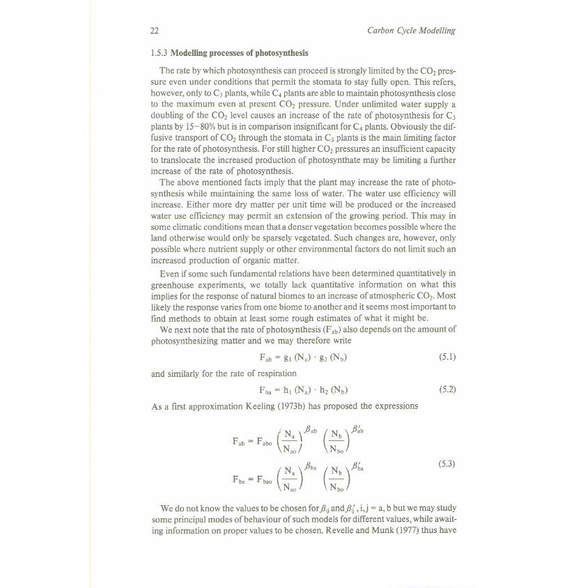
The rate bywhich photosynthesis can proceed is stronglylimited bythe CO2pres-sure even under conditions that permit the stomata to stay fully open. This refers,however, only to C3plants,while C4plants are able to maintain photosynthesis closeto the maximum even at present CO2 pressure. Under unlimited water supply adoubling of the CO2 level causes an increase of the rate of photosynthesis for C3plants by 15-80% but is in comparison insignificantfor C4plants. Obviouslythe dif-fusive transport of CO2through the stomata in C3 plants is the main limiting factorfor the rate of photosynthesis. For stillhigher CO2pressures an insufficient capacityto translocate the increased production of photosynthate may be limiting a furtherincrease of the rate of photosynthesis.

The above mentioned facts imply that the plant may increase the rate of photo-synthesis while maintaining the same loss of water. The water use efficiency willincrease. Either more dry matter per unit time will be produced or the increasedwater use efficiency may permit an extension of the growing period. This may insome climatic conditions mean that a denser vegetationbecomes possiblewhere theland otherwise would only be sparsely vegetated. Such changes are, however, onlypossible where nutrient supply or other environmental factors do not limit such anincreased production of organic matter.

Even if some such fundamental relations have been determined quantitatively ingreenhouse experiments, we totally lack quantitative information on what thisimplies for the response of natural biomes to an increase of atmospheric CO2.Mostlikelythe response variesfrom one biome to another and it seems most important tofmd methods to obtain at least some rough estimates of what it might be.

We next note that the rate of photosynthesis (Fab)also depends on the amount ofphotosynthesizing matter and we may therefore write

Fab = gl (Na) . g2 (Nb)

and similarly for the rate of respiration

(5.1)

Fba = hI (Na) . h2 (Nb)

As a first approximation Keeling (1973b)has proposed the expressions

(5.2)

We do not know the values to be chosen forflij andfli) , i,j = a, b but we may studysome principal modes of behaviour of such models for different values, while await-ing information on proper values to be chosen. Revelle and Munk (1977) thus have

Fab = Fabo (Na \flab (Nb) flbNao! Nbo

F F (N.t. (N.t""(5.3)

ba bao-Nao Nbo


shown that forfi~b= fiba and for a given input of CO2 into the atmosphere, a new equi-librium will be reached when all the excess has been transferred to the biota. Kohl-

maier (chapter 5, this volume) has studied the general stability properties of biota sys-

tems for various choices of the values for flij and fiif , i, j = a, b in eq (5.3).

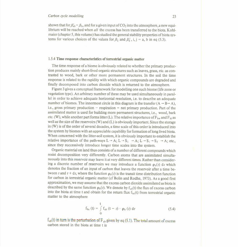
1.5.4Time response characteristics ofterrestrial organicmatter

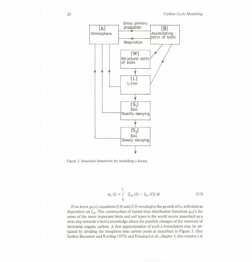
The time response of a biome is obviouslyrelated to whether the primary produc-tion produces mainly short-livedorganic structures such as leaves,grass,etc. as con-trasted to wood, bark or other more permanent structures. In the soil the timeresponse is related to the rapiditywith which organic compounds are degraded andfmally decomposed into carbon dioxide which is returned to the atmosphere.

Figure 3givesa conceptual framework for modellingone such biome (lifezone orvegetation type). An arbitrary number of these may be used simultaneously in paral-lel in order to achieve adequate horizontal resolution, i.e. to describe an adequatenumber of biomes. The innermost circle in this diagram is the transfer (A --+B--+ A),

i.e., gross primary production - respiration = net primary production. Part of theassimilated matter is used for building more permanent structures, i.e., wood, barketc. (W), while another part forms litter (L). The relative importance ofF bwand FbIaswell as the size ofthe reservoirs (W) and (L) is obviously important. Since the storagein (W) is of the order of several decades, a time scale of this order is introduced intothe system by biomes with an appreciable capability for formation oflong lived biota.When concerned with the litter-soil system, it is obviously important to establish therelativeimportanceof the path-waysL --+A; L --+Sl --+A; L --+Sl --+S2 --+A; etc.,since they successively introduce longer time scales into the system.

Organic material on land thus consists of a number of different compounds whichresist decomposition very differently. Carbon atoms that are assimilated simulta-neously into this reservoir may leave it at very different times. Rather than consider-ing a discretenumber of reservoirswe may introducea functionqJb(T)dT whichdenotes the fraction of an input of carbon that leaves the reservoir after a time be-tween Tand T+ dT, where the function qJb(T)is the transit time distribution function

for carbon in terrestrial organic matter (cf Bolin and Rodhe, 1973). As a good fIrstapproximation, we may assume that the excess carbon dioxide assimilated as biota is

described by the same function qJb(T).We denote by fab(t)the flux of excess carboninto the biota at time t and obtain for the return flux fba(t)from terrestrial organicmatter to the atmosphere

t

fba (t) = Jfab (t - T) . qJb(T) dT0

(5.4)

fab(t)in turn is the perturbation ofF ab given by eq (5.1).The total amount of excesscarbon stored in the biota at time t is


(A)Atmosphere

Grossprimoryprod~uction I (B)

Assimilatingparts of biota

Respiration

(W)Structuralpartsof biota

(51)Soil

Rapidlydecoying

(52)Soil

Slowlydecaying

Figure 3: Structural framework for modelling a biome.

t

nb (t) = J [fab(1') - fba (1')] d1'0

(5.5)

Ifwe knew (]Jb(T),equations (5.4)and (5.5)would givethe growth ofnb with time asdependent on fab.The construction of transit time distribution functions (]Jb(T)forsome of the more important biota and soil types in the world seems important as anext step towards a better knowledgeabout the possible changes of the reservoir ofterrestrial organic carbon. A fIrstapproximation of such a formulation may be ob-tained by dividing the biosphere into carbon pools as described in Figure 3. (Seefurther Bacastow and Keeling (1973)and Emanuel et aI.,chapter 5, this volume.) A


more explicit attempt in this direction is formulated by Moore et al. (chapter 5, thisvolume). Based on available data they deduce response functions for the biomeslisted in section 5.2 above, analyze in detail man's likely interference with thesenatural systems and try to determine the total net fluxof carbon dioxide to the atmo-sphere since 1860.The possible changes of the rate of photosynthesis due to theincreasing atmospheric CO2 concentration was not considered and the determina-tion of the net CO2 exchange between the terrestrial system and the atmosphereremains unresolved. The method developed by Moore et al. is, however, useful inorder to incorporate new data into models of the carbon cycle.It alsopermits experi-mentation regardingthe importance of different ideas on the dependance of the rateof photosynthesis on atmospheric CO2 or nutrient availabilityand also the role ofrespiration and bacterial decomposition in the soil.

REFERENCES

Arons, A.B., Stommel, H. (1967).On the abyssal circulation of the World Ocean- III. Anadvection-lateral mixing model of the distribution of a tracer property in an ocean basin.Deep Sea Res. 14,441-458.

Bacastow, R. (1976).Modulation of atmospheric carbon dioxide by the Southern Oscilla-tion, Science, 261, 116-118.

Bacastow,R. and Keeling, C.D. (1973).Atmospheric carbon dioxide and radiocarbon in thenatural carbon cycle: Changes from A.D. 1700to 2070 as deduced from a geochemicalmodel. In Woodwell, G.M. and Pecan, E.V. (Eds.) Carbon and the Biosphere. AECSymposium Series 30, 86-135, US Dept of Commerce, Springfield,Virginia.

Bathen, K.H. (1972).On the seasonal changes in depth of the mixed layerin the North PacificOcean. J. Geoph. Res., 77,7138-7150.

Berger,R. and Libby,W.F. (1969).Equilibrium of atmospheric carbon dioxidewith seawater:Possible enzymatic control of the rate. Science, 164, 1395-1397.Bischof, W. (1977).Comparability of CO2 measurements. Tellus, 29, 435-444.Bj6rkstr6m, A. (1979).A model of CO2 interaction between atmosphere, oceans, and land

biota. In: Bolin, B. et al. (Eds.) The Global Carbon Cycle, 403-457. John Wiley & Sons,Chichester.

Bolin, B. (1960).On the exchange of carbon dioxide between the atmosphere and the sea.Tellus, 12, 274-281.

Bolin,B.(1977).Changes ofland biota and their importancesfor the carbon cycle.Science,196,613-615.

Bolin, B. and Eriksson, E. (1959).Changes of the carbon dioxide content of the atmosphereand sea due to fossil fuel combustion. In: Bolin, B. (Ed.) Atmosphere and Sea in Motion,130-142. The Rockefeller Institute Press.

Bolin, B. and Keeling, C.D. (1963).Large-scale atmospheric mixing as deduced from theseasonal and meridional variations of carhon dioxide. J. Geophys. Res., 68, 3899-3920.

Bolin, B. and Rodhe, H. (1973).A note on the concept of age distribution and transit time innatural reservoirs. Tellus, 25, 58-62.

Bolin, B., Degens, E.T., Duvigneaud, p, and Kempe, S. (1979),The global biogeochemicalcarbon cycle.In: Bolin, B. et al. (Eds.) The Global Carbon Cycle, SCOPE 13, 1-56, JohnWiley & Sons, Chichester.


Bray,J.R. (1959).An analysisof the possible recent change in atmosperic carbon dioxide con-centration. Tellus, 11,220-230.

Broecker,W.S.(1979).A revisedestimatefor the radiocarbon ageofNorth Atlantic deep water.J. Geophys. Res., 84, 3218-3226.

Broecker, W.S., Li, Y.-H., Peng, T.-H (1971). Man's artifact. In: Hood, D.w. (Ed.)Impingement of Man on the ocean, 287- 324.Wiley-Interscience,New York.

Broecker,W.S.,Peng, T.-H. (1974).Gas exchange rates between airand sea. Tellus,26,21- 35.Broecker, W.S., Peng, T.-H., Stuiver, M. (1978).An estimate of the upwelling rate in the

equatorial Atlantic based on the distribution of bomb radiocarbon. J. Geophys. Res., 83,6179-6186.

Broecker, W.S., Takahashi, T., Simpson, H.J., Peng, T.-H. (1979).Fate of fossil fuel carbondioxide and the global carbon budget. Science, 206,409-418.

Bryan, K. (1969).A numerical method for the study of the circulation of the world ocean. J.Comput. Phys., 4,347-376.

Buch, K., Harvey, H.W., Wattenberg,H. and Gripenberg, S. (1932).Ueber das Kohlensiiure-system in Meerwasser. Raports et Proces-Verbaux des Reunions, ICES 79, 1-70.

Buch, K. (1951).Das Kohlensiiure Gleichgewichtssystemim Meerwasser: Kritische Durch-sicht und Neuberechnungen der Konstituenten. HavsforskningsinstitutetsSkrift,151,1-18.

Callendar, G.S. (1958). On the amount of carbon dioxide in the atmosphere Tellus, 10,243-248.

Craig, H. (1957).The natural distribution of radiocarbon and the exchange time of carbondioxide between atmosphere and sea. Tellus, 9, 1-17.

Craig,H. (1969).Abyssalcarbon and radiocarbon in the Pacific.J. Geoph. Res., 74,5491-5506.Freyer, H.-D. (1979).Variationsin the atmospheric CO2content. In: Bolin, B. et at.(Eds.) The

Global Carbon Cycle, SCOPE 13,79-99, John Wiley & Sons, Chichester.Gordon, A.L. (1975).General ocean circulation. In: Reid, R.O. (Ed) Numerical models of

ocean circulation, 39-53, National Academy of Science, Washington, D.C.Gunther, P.R. (1978).Sea water equilibration experiment. Report 78-14. ScrippsInstitution,

La Jolla, California.Hampicke, U. (1979).Net transfer of carbon between the land biota and the atmosphere,

induced by man. In: Bolin, B. et al. (Eds.) The global carbon cycle. SCOPE 13,219-236.John Wiley & Sons, Chichester.

Hansson, I. (1973).A new set of acidityconstants for carbon acid and boric acid in sea water.Deep Sea Research, 20, 461-478.

Holland, W.R. (1971).Ocean tracer distributions.Part I. A preliminarynumerical experiment.Tellus, 23, 371- 391.

Jiihne, B., Munnich, K.O., Siegenthaler, U. (1979). Measurements of gas exchange andmomentum transfer in a circular wind-water tunnel. Tellus, 31, 321-329.

Junge, C., Czeplak, G. (1968).Some aspects of the seasonal variation of carbon dioxideand ozone. Tellus, 20, 422-434.

Keeling, C.D. (1973a). Industrial production of carbon dioxide from fossil fuels andlimestone. Tellus, 25, 174-198.

Keeling, C.D. (1973b).The carbon dioxide cycle. Reservoir models to depict the exchangeof atmospheric carbon dioxide with the oceans and land plants. In: Rasool, S. (Ed.)Chemistry of the Lower Atmosphere, 251-329. Plenum Press, New York.

Keeling, C.D. (1980).The Suess effect: 13Carbon _14Carbon interrelations. EnvironmentalInternational 2 (in press).

Keeling, CD. and Bolin, B. (1967).The simultaneous use of chemical tracers in oceanicstudies. I: General theory of reservoir models. Tellus, 19, 566-581.

Keeling, C.D. and Bolin, B. (1968).The simultaneous use of chemical tracers in oceanicstudies. II: A three reservoir model of the North and South Pacific Oceans. Tellus, 20,17-54.


Keeling, C.D. and Bacastow, R.B. (1977).Impact of industrial gases on climate. In: Energyand Climate. Stud. Geophys., 72-95. Nat. Acad. of Sciences, Washington, D.C.

Keeling, e.D., Gunther, P.R. (1977).The thermodynamic ionization constants of carbonicacid, Report 77-24. Scripps Oceanographic Institution, La Jolla, California.

Keeling, e.D., Mook, W.G. and Tans, P.P. (1979).Recent trend in the 13C/l2C ratio ofatmospheric carbon dioxide. Nature, 277, 121-123.

Keeling, C.D. (1979). The Suess Effect: 13Carbon-14CarbonInterrelations. EnvironmentInternational, 2, 229- 300.

Keeling, e.D., Bacastow, R.B., Tans, P.P. (1980). Predicted Shift in the 13C/l2C ratio ofatmospheric carbon dioxide. Geophysical Research Letters, 7, 505-508.

Krey, P.W., Schonberg, M. and Tonnkel, L. (1974).Updating stratospheric inventories toJanuary 1973.Rep. HASL-281, 1/30-1/42, USAEC, New York.

Kuo, H. and Veronis, G. (1970).Distribution of tracers in the deep oceans of the world.Deep-Sea Res., 17, 29-46.

Lerman, J.e., Mook, W.G., and Vogel,J.C. (1970).14Cin tree rings from different localities.In I.V. Olsson (Ed.) Radiocarbon variations and absolute chronology. Almqvist &Wiksell, Stockholm.

Lyman, J. (1957). Buffer mechanism of sea water. Thesis University of California LosAngeles.

Machta, L. (1972).The role of the oceans and the biosphere in the CO2 cycle. In: Dyrssen,D. (Ed.), Changing Chemistry of the Oceans. Nobel Symposium, No 20, Almqvist &Wicksell, Stockholm.

Machta, L. (1973).Prediction of CO2 in the atmosphere. In Woodwell,G.M. and Pecan, E.V.

(Eds.) Carbon in the Biosphere. AEC Symposium Series 30121-31, NTIS U.S. Dept.of Commerce, Springfield,Virginia.

Mehrbach, C., Culberson, C.H., Hawley, J.E. and Pytkowicz,R.M. (1973).Measurementsof the apparent dissociation constants of carbonic acid in sea water at atmosphericpressure. Limnology Oceanography, 18, 897-907.

Menard, H.W., Smith, S.M. (1966).Hypsometry of ocean basin provinces. J. Geoph. Res.,71,4305-4325.

Mopper, K. and Degens, E.T. (1979). Organic carbon in the ocean: Nature and cycling.In: Bolin, B. et a/. (Eds.) The global carbon cycle, SCOPE 13, 293-316, John Wiley &Sons, Chichester.

Munk, W.H. (1966).Abyssal recipes. Deep Sea Res., 13, 707-730.Munk, W., Ruderman, M., Zachariasen, F. (1979).The oceans as a sink for carbon dioxide.

Jason Report to VS DOE, Washington.Newell, R.E., Nawato, A.R., Husing, J. (1978).Long term global sea surface temperature

fluctuations and their possible influence on atmospheric CO2 concentration. Pure andApplied Geophysics, 116, 351 ~ 371.

Nydal, R., L6vseth, K., Gulliksen, S. (1972).A survey of radiocarbon variations in naturesince the Test Ban Treaty. Proc. 9th Int. Radiocarbon Conf. Univ. of Calif, Los Angeles.

Oeschger, H., Siegenthaler, V., Schotterer, V., and Gugelmann, A. (1975).A box diffusionmodel to study the carbon dioxide exchange in nature. Tellus, 27, 168-192.

Oeschger, H., Siegenthaler, V. and Heimann, M. (1980).The carbon cycle and its perturba-tion by man (to be published).

Pearman, G.I., Francy, R.G. and Fraser, P.I. (1976).Climate implications of stable carbonisotopes in tree rings. Nature, 260,771-772.

Pearman, G.I., and Hyson, P. (1980). Activities of the global biosphere as reflected inatmospheric CO2 records. J. Geophysical Res., 85, 4457-4467.

Peng, T.-H., Broecker, W.S., Mathieu, G.G. and Li, Y.-H. (1979).Radon evasion rates inthe Atlantic and Pacific Oceans as determined during the Geosecs program. 1. Geophys.Res., 84, 2471-2486.


Reiter, E.R. (1975). Stratospheric-tropospheric exchange processes. Rev. Geophys. andSpacePhys.,13,459-474.

Revelle, R. and Suess, H. (1957).Carbon dioxide exchange exchange between atmosphereand ocean and the question of an increase of atmospheric CO2 during the past decades.Tellus, 9, 18-27.

Revelle, R. and Munk, W. (1977).The carbon dioxide cycle and the biosphere. In: Energyand Climate. Stud. Geophys., 140-158. Nat. Acad. of Sciences, Washington, D.C.

Rooth, c., Ostlund, G. (1972).Penetration of tritium into the Atlantic thermocline. DeepSea Res.

Schlesinger, W.H. (1977).Carbon balance in terrestrial detritus. Ann. Ecol. Syst., 8, 51-81.Schlesinger, W.H. (1979).The world carbon pool in soil organic matter. In: Woodwell,G.M.

(Ed.) The role of terrestrial vegetation in the global carbon cycle. Methods forappraising changes. SCOPE Report (to be published) Wiley, New York.

Siegenthaler, D., Heimann, M. and Oeschger, H. (1978).Model response of the atmosphericCO2 level and l3CfI2C ratio to biogenic CO2 input. IIASA Workshop on carbon dioxide,climate and society. IIASA Laxenburg, Austria.

Siegenthaler, D. and Oeschger, H. (1978). Predicting future atmospheric carbon dioxidelevels. Science, 199,388-395.

Siegenthaler, u., Heimann, M. and Oeschger, H. (1980). 14Cvariations caused by changesin the global carbon cycle. Proc. 10th Int.Radiocarbon Conference. Radiocarbon, 22,177-191.

Stuiver, M. and Polach, H. (1977).Reporting of 14Cdata. Radiocarbon, 19, 355-363.Stuiver,M. (1978).Atmospheric carbon dioxide and reservoir changes.Science, 199,253-258.Stuiver, M. and Quay, P.D. (1980 a). Changes in atmospheric carbon-14 attributed to a

variable sun. Science, 207, 11-19.Stuiver, M. (1980b). 14Cdistribution in the Atlantic Ocean. J. Geoph. Res., 85, 2711-2718.Suess, H.E. (1965).Secular variationsof the cosmic-ray-producedcarbon-14in the atmosphere

and their interpretation. J. Geophys. Res., 70, 5937-5952.Suess, H. (1970).The three causes of the secular CI4 fluctuations and their time constants.

In: Olsson I (Ed.) Radiocarbon Variations and Absolute Chronoly. Nobel SymposiumNo 12.Almqvist & Wicksell, Stockholm.

Tans, P. (1979). Carbon-13 and carbon-14 in trees and the atmospheric CO2 increase.Proefschrift, Rijksuniversiteit, Groningen.

Veronis, G. (1975).The role of models in tracer studies. In: Numerical models of oceancirculation, 133-146. National Academy of Sciences, Washington, D.C.

Wagener, K. (1979).The carbonate system of the ocean. In: Bolin, B. et al. (Eds.) The globalCarbon Cycle, SCOPE 13,251-258 John Wiley & Sons, Chichester.

Walin, G. (1977).A theoretical framework for description of estuaries Tellus, 29, 128- 136.Welander, P. (1971). The thermocline problem. Philos. Trans. R. Soc. London Ser A,

270,69-73.Whittaker, R.H., Likens, G.E. (1975).The biosphere and man. In: Leeth, H. and Whittaker,

R.H. (Eds.). Primary productivity of the biosphere. Ecol. Stud. 14, 305-328. SpringerVerlag, Berlin, Heidelberg, New York.

Wilson, A.T. and Grinsted, MJ. (1977). l3CfI2C in cellulose and lignin as paleo-thermo-meters. Nature, 265, 133- 135.

Woodwell, G.M., Whittaker, R.H. Reimers, W.A., Likens, G.E., Delwiche, C.C., andBotkin, D.B. (1978).The biota and the world carbon budget. Science, 199, 141-146.

Wyrtki, K. (1962).The oxygen minima in relation to ocean circulation Deep Sea Res., 9,11-23.

chapter 1 carbon cycle modelling - carnegie ecology€¦ · · 2016-12-22chapter 1 carbon cycle...

Documents