Earth Observation Data and Carbon Cycle Modelling

Marko ScholzeQUEST, Department of Earth Sciences

University of Bristol

GAIM/AIMES Task Force Meeting, Yokohama, 24-29 Oct. 2004

(an incomplete and subjective view…)

Overview

• Atmospheric CO2 observations– TransCom

• Model-Data Synthesis– Oceanic DIC observations: Inverse Ocean

Modelling Project– Terrestrial observations: Eddy-flux towers– Atmospheric observations: Carbon Cycle Data

Assimilation system

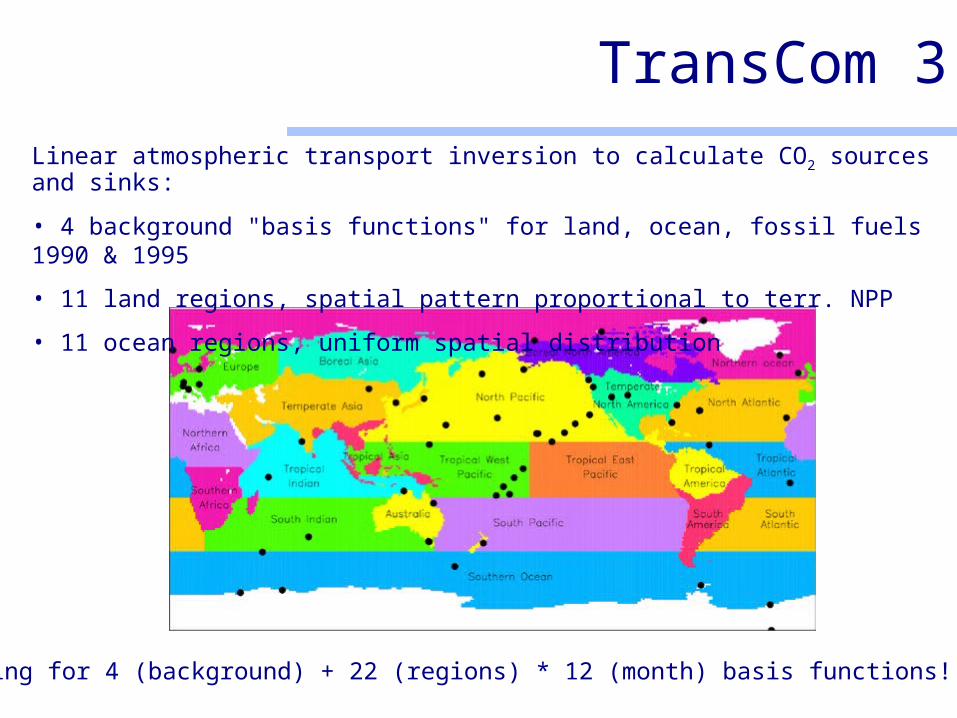
TransCom 3Linear atmospheric transport inversion to calculate CO2 sources and sinks:

• 4 background "basis functions" for land, ocean, fossil fuels 1990 & 1995

• 11 land regions, spatial pattern proportional to terr. NPP

• 11 ocean regions, uniform spatial distribution

Solving for 4 (background) + 22 (regions) * 12 (month) basis functions!

TransCom 3 Seasonal Results(mean over 1992 to 1996)

Guerney et al., 2004

response to background fluxes:

ppm

inversion results:

-35

15 4

-5

Gt

C/y

r

TransCom 3 Interannual Results (1988 - 2003)

red: landblue: ocean

darker bands: within-modeluncertainty

lighter bands: between-model uncertainty

• larger land than ocean variability• interannual changes more robust than seasonal

... but atmosphere well mixed interannually... Baker et al. 2004

Gt

C/y

r

Model-Data Synthesis:The Inverse Ocean Modelling

Project

C* of Gruber, Sarmiento, and Stocker (1996) to estimate anthropogenic DIC.Innumerable data authors, but represented by Feely, Sabine, Lee, Key.

Recent ocean carbon survey, ~ 60.000 observations

The Inverse Ocean Modelling Project

Jacobson, TransCom3Meeting, Jena, 2003

The Inverse Ocean Modelling Project

Gloor et al. 2003

• southward carbon transport of 0.37 Pg C/yr for pre-industrial times• present-day transport -0.06 Pg C/yr (northwards)

Terrestrial observations: Fluxnet a global network of eddy covariance

measurements

Inversion of terrestrial ecosystem parameter values against eddy covariance

measurements by Metropolis Monte Carlo sampling

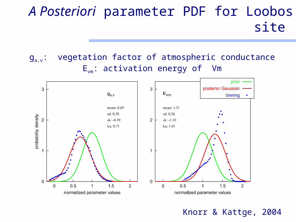
A Posteriori parameter PDF for Loobos site

ga,v: vegetation factor of atmospheric conductanceEvm: activation energy of Vm

Knorr & Kattge, 2004

Carbon sequestration at the Loobos site during 1997 and 1998

Knorr & Kattge, 2004

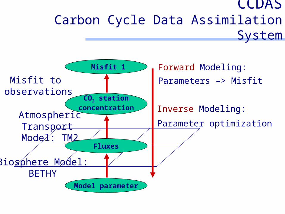
CCDASCarbon Cycle Data Assimilation System

CO2 stationconcentration

Biosphere Model:BETHY

Atmospheric Transport Model: TM2

Misfit to observations

Model parameter

Fluxes

Misfit 1 Forward Modeling:

Parameters –> Misfit

Inverse Modeling:

Parameter optimization

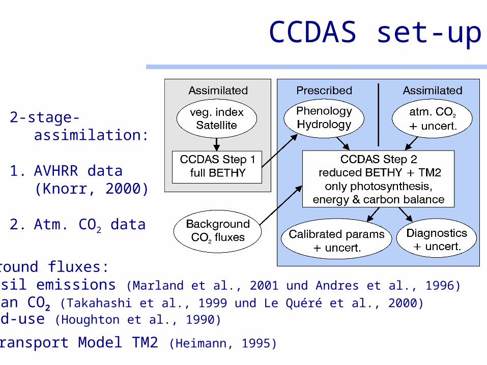
CCDAS set-up

2-stage-assimilation:

1. AVHRR data(Knorr, 2000)

2. Atm. CO2 data

Background fluxes:1. Fossil emissions (Marland et al., 2001 und Andres et al., 1996)2. Ocean CO2 (Takahashi et al., 1999 und Le Quéré et al., 2000)3. Land-use (Houghton et al., 1990)

Transport Model TM2 (Heimann, 1995)

Methodology

Minimize cost function such as (Bayesian form):

[ ] [ ] [ ] [ ]DpMDpMpp pppJ D

T

pT rrrrrrrrrrr

−−+−−= )()()( 2

1

2

1 10

10 0

-- C C

where- is a model mapping parameters to observable quantities- is a set of observations- error covariance matrixC

DrMr

pr

need of (adjoint of the model)Jpr∇

1

2

2−

⎪⎭

⎪⎬⎫

⎪⎩

⎪⎨⎧

≈ji,

p pJ

rr

∂∂

C

Uncertainties of parametersT

pX p)p(X

p)p(X

rrr

rrr

rr

∂∂

∂∂

≈ CC

Uncertainties of prognostics X

Figure from Tarantola, 1987

Gradient Method

1st derivative (gradient) ofJ (p) to model parameters p:

yields direction of steepest descent.

pr

pr

ppJrr

∂∂− )(

cost function J (p) pr

Model parameter space (p)pr

2nd derivative (Hessian)of J (p):

yields curvature of J.Approximates covariance ofparameters.

pr

22 ppJrr

∂∂ )(

Data Fit

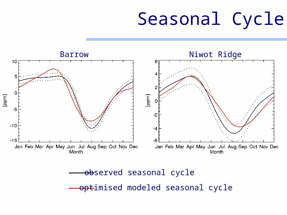
Seasonal Cycle

Barrow Niwot Ridge

observed seasonal cycle

optimised modeled seasonal cycle

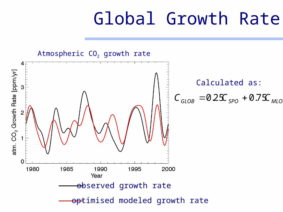
Global Growth Rate

Calculated as:

observed growth rate

optimised modeled growth rate

Atmospheric CO2 growth rate

MLOSPOGLOB CCC 75.025.0 +=

Error Reduction in Parameters

Relative Error Reduction

Carbon Balance

latitude N*from Valentini et al. (2000) and others

Euroflux (1-26) and othereddy covariance sites*

net carbon flux 1980-2000gC / (m2 year)

IAV and processes

Major El Niño events

Major La Niña event

Post Pinatubo period

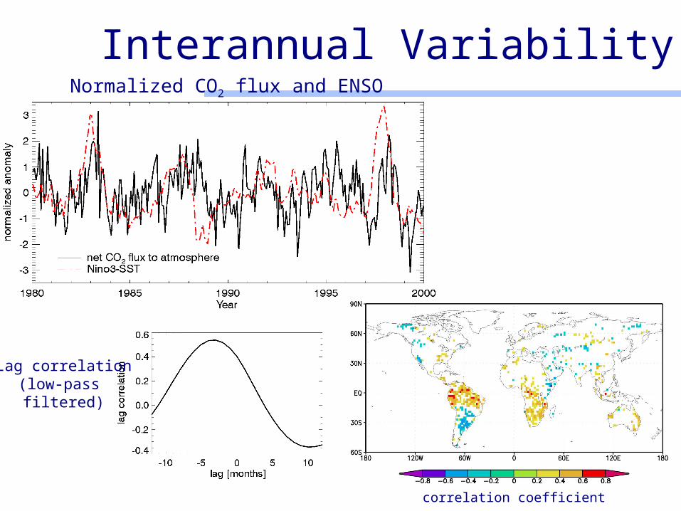
Interannual VariabilityNormalized CO2 flux and ENSO

Lag correlation(low-pass filtered)

correlation coefficient

Outlook

• Data assimilation: problem better constrained without "artefacts" (e.g. spatial patterns created by station network)

but: cannot resolve processes that are not included in the model (look at residuals and learn about the model)

• Simultaneous inversion of land and ocean fluxes• Isotopes• More data over tropical lands: satellites

• Model-Data-Synthesis: problem better constrained without "artefacts" (e.g. spatial patterns created by station network)

but: cannot resolve processes that are not included in the model (look at residuals and learn about the model)

• Simultaneous inversion of land and ocean fluxes

• Further data constraints (e.g. Isotopes, Inventories)

• More data over tropical lands: satellites

Posterior Uncertainty in Net Flux

Uncertainty in net carbon flux 1980-200gC / (m2 year)

Uncertainty in prior net flux

Uncertainty in net carbon flux from prior values 1980-2000gC / (m2 year)

Atm. Inversion on Grid-cell

• prior and posterior uncertainties• sensitivities (colors)

Rödenbeck et al. 2003

Atm. Inversion on Grid-cell

prior/posterior fluxesand reduction in uncertaintyRödenbeck et al. 2003

Not really at model grid of TM3, but aggregated to TM2 grid, 8° x 10°,Underdetermined problem correlation matrix (e.g. l=1275 km for NEE)

CO2 Satellite Measurements

Vertical weighting functions

Sciamachy, OCO

Airs (U) (=Upper limit)

Airs (L) (=Lower limit)

Houweling et al. 2003

Pseudo Satellite Data Inversion

posterior/prior uncertainty

Houweling et al. 2003