chapter 1: angular momentum algebra ii
TRANSCRIPT

Introduction
Chapter 1: Angular Momentum Algebra II
Prof. Alok Shukla
Department of Physics
IIT Bombay, Powai, Mumbai 400076
Course Name: Quantum Mechanics II (PH 422)
Shukla Angular Momentum

Summary of the Chapter
In this chapter, �rst we will brie�y review what you have learnt inangular momentum algebra in the �rst part of this course. Afterthat, we will discuss rotation operators and their representations.The theory will be developed for rotations about general axes, andwill make use of the Euler angles. Next important topic will be theaddition of angular momenta using the Clebsch-Gordonmethodology. For the purpose, the concept of tensor productspaces will be introduced, and the operations of direct sum anddirect products will be de�ned. Using the theory developed,Wigner-Eckart theorem, and its corollary, projection theorem will beproved. Finally, the applications of these concepts will be discussedin various problems in the tutorial sheets.

Introduction
Introduction
You studied the basics of angular momentum algebra in theprevious course (Q. Mech. I), last semester
We will �rst brie�y review that
This will be followed by a discussion of rotation operators andtheir representations
Next, we will introduce the concept of tensor-product spaces
This will allow us to develop the theory of the addition ofangular momenta
Finally, we will prove the Wigner-Eckart theorem, and discussits consequences
Shukla Angular Momentum

Introduction
Review of the basics
The angular momentum operator J is Hermitian vectoroperator de�ned as
J = Jx i +Jy j +Jz k , (1)
where Jx , Jy , and Jz are its three Cartesian components.
The Hermiticity condition
J = J†, (2)
implies that the individual components are also Hermitian
Jx = J†x ; Jy = J†
y ; Jz = J†z (3)
Shukla Angular Momentum

Introduction
Review of basics...
Additionally, the three components of the angular momentummust satisfy the commutation relations
[Jx ,Jy ] = i hJz
[Jy ,Jz ] = i hJx
[Jz ,Jx ] = i hJy
(4)
Which can be written in the compact form
[Ji ,Jj ] = i hεijkJk (5)
Using these commutation relations, one can show that theoperator J2 = J2x +J2y +J2z , with each individual angularmomentum component [
J2,Ji]
= 0 (6)
Shukla Angular Momentum

Introduction
Angular Momentum Algebra (contd.)
Eq. 6 implies that J2 and Ji are simultaneously diagonalizable,i.e., they have common eigenvectors
But, because di�erent components of J do not commute witheach other (see Eq. 5), we cannot �nd their simultaneouseigenvectors
Thus, by convention, we work with the simultaneouseigenvectors of J2 and Jz , labeled |jm〉, satisfying
J2|jm〉= j(j +1)h2|jm〉Jz |jm〉= mh|jm〉, (7)
where −j ≤m ≤ j .
Kets |jm〉 form an orthonormal set⟨j ′m′ | jm
⟩= δj ′ jδm′m. (8)
Shukla Angular Momentum

Introduction
Angular Momentum Algebra Revision...
One can also show that the allowed values of j are
j = 0,1
2,1,
3
2,2, . . . , (9)
and that successive m for a given j di�er by one, i.e.,m′ = m±1
Combining this with that fact that −j ≤m ≤ j , we concludethat for a given value of j , there are 2j +1 allowed values ofm, given by
−j ,−j +1,−j +2, . . . , j−2, j−1, j
Now, the question arises, what is the action of Jx and Jyoperators on the ket |jm〉?To perform these calculations, it helps to de�ne the ladderoperators
J± = Jx ± iJy . (10)
Shukla Angular Momentum

Introduction
Angular momentum algebra revision...
It is easy to verify that the ladder operators are not Hermitian
J†± = J∓. (11)
One can write J2 operator in terms of them
J2 =1
2(J+J−+J−J+) +J2z . (12)
Using the commutation relations (Eq. 5) one can show that
J+|jm〉=√
(j−m)(j +m+1)h | jm+1〉J−|jm〉=
√(j +m)(j−m+1)h|jm−1〉.
Or in short
J±|jm〉=√
(j∓m)(j±m+1)h | jm±1〉 (13)
Shukla Angular Momentum

Introduction
Revision of Angular Momentum Algebra
In other words the action of J+/J− on kets |jm〉 leaves junchanged, but increments/decrements the m values by one.
Using Eqs. 13 and 10, one can easily obtain the action ofJx/Jy operators on the ket |jm〉It is fruitful to make the following comment at this stage
Ji s refer to the Cartesian components of a general angularmomentum operator
In practice, Ji could be the orbital angular momentumoperator Li , or the spin angular momentum operator Si , or thesum Li +Si of the two.
Or it could refer to an entirely di�erent kind of angularmomentum
Any operator which satis�es the commutation relations of Eq.5, will have the properties of a quantum angular momentumoperator
Shukla Angular Momentum

Introduction
Generator of Rotation
Let us consider a general vector V, which could represent anyvectorial physical quantity such as position r, momentum p etc.
We will be interested in studying how a given vectortransforms under a rotation
For rotations, we can adopt a �passive� view or an �active�view.
Under the �passive� view, the coordinate system (i.e. thecoordinate axes) are rotated, keeping the vector �xed, andthen we study how the vector transforms as a result
In the �active� view, on the other hand, we hold the coordinatesystem �xed, and rotate the vector instead, and study itstransformation properties
Shukla Angular Momentum

Introduction
Generator of Rotation...
Let us consider a system with Hamiltonian H
We rotate the position vector r by an angle φ about an axisoriented along the direction n.
That is, we are adopting an active view of rotations.
Let R denote the operator representing this rotation, underwhich r→ r′
r′ = Rr
As a result, in the r-representation, the Hamiltonian operatorH(r), as well as a general wave function α(r) also transform
H(r) → H ′(r′)α(r) → α ′(r′)
(14)
One can de�ne these transformations using a unitary operatorcorresponding to the rotation R
Shukla Angular Momentum

Introduction
Generator of Rotation...
In the state space (Dirac representation), the correspondingunitary operator is denoted as UR
Its action on the Hamiltonian H and a general ket |α〉 is givenby
HR = URHU†R
|α〉R = UR |α〉.(15)
Note that HR and |α〉R are the corresponding transformedquantities after the rotation R has been performed.
Eqs. 15 are the state space counterparts of Eqs. 14.
One can show that the unitary operator UR is given by
UR = e−ihJ·nφ , (16)
where J is the vector angular momentum operator de�nedearlier.
Shukla Angular Momentum

Representation of the Rotation Operator
Because J appears in the formula of the rotation operator, it iscalled the generator of rotations
This is similar to the unitary operator U(r) which de�nes atranslation by a vector r
U(r) = e−ihp·r,
where p is the linear momentum operator.
Thus, p is said to be the generator of translations.
We know from linear algebra that the matrix corresponding toa linear operator in a vector space, with respect to a chosenbasis, is called its representation
We are interested in obtaining the representation of the UR
operator in the state space, with respect to the basis{|jm〉,m =−j , . . . j}

Rotation Matrices...
The matrices representing UR with respect to the chosen basisare called rotation matrices
Let us obtain the expressions for the elements of the rotationmatrices
Using the resolution of identity (∑jm′=−j |jm
′〉〈jm′|= I ), weobtain
UR |jm〉=j
∑m′=−j
∣∣jm′⟩〈jm′ |UR | jm〉.
De�ning the rotation matrix elements as
D(j)m′m(R) =
⟨jm′ |UR | jm
⟩=⟨jm′∣∣∣e− i
hJ·nφ
∣∣∣ jm⟩ , (17)
we obtain
UR |jm〉=j
∑m′=−j
D(j)m′m(R)|jm′〉. (18)

Rotation matrices...
From Eq. 17 it is obvious that the elements D(j)m′m(R) de�ne
the representation of the rotation operator with respect to thechosen basis, i.e., the rotation matrices.
It is obvious that computing D(j)m′m(R) for the most general
rotation will be complicated
However, for a rotation about the z axis (n = k), the matrixelements have a very simple form, as derived below
D(j)m′m(R) =
⟨jm′∣∣∣e− i
hJ·nφ
∣∣∣ jm⟩=⟨jm′∣∣∣e− i
hJzφ
∣∣∣ jm⟩=⟨jm′∣∣∣e− i
hmhφ
∣∣∣ jm⟩= e−imφ
⟨jm′|jm
⟩= e−imφ
δm′m.

Rotation matrices through Euler Angles
In the derivation we used the relation
f (Jz)|jm〉= f (mh)|jm〉,
where f (Jz) is an analytic function of Jz .
The result can be easily proved by making a Taylor expansionof f (Jz), and the fact Jz |jm〉= mh|jm〉.Rotations about a general axis can be simpli�ed a great dealby borrowing the concept of Euler angles from rigid-bodydynamics
Using the concept of Euler angles or Euler rotations, a generalrotation can be expressed in terms of three counter-clockwiserotations by angles α , β , and γ (called Euler angles)
The �rst rotation by angle α is about the original z axis
The second one by angle β is about the new y axis
The �nal one by angle γ is about the new z axis.

Introduction
Rotation matrices using Euler angles...
Note that here we are rotating the coordinate system, whichmeans these are �passive� rotations
If the initial axes are de�ned as (x ,y ,z), intermediate ones by(x ′′,y ′′,z ′′), and the �nal ones by (x ′,y ′,z ′), then it is obvious
UR = e−ih
γ z ′·Je−ih
β y ′′·Je−ih
α z ·J. (19)
Using the following mathematical trick, one can transform UR
into a form which involves rotations only about the original(unprimed) axes.
The involves the realization
e−ih
β y ′′·J = e−ih
α z ·Je−ih
β y ·Jeih
α z ·J, (20)
Shukla Angular Momentum

Introduction
Rotation matrixes using Euler angles...
ande−
ih
γ z ′·J = e−ih
β y ′′·Je−ih
γ z ·Jeih
β y ′′·J. (21)
On substituting Eqs. 20 and 21 in Eq. 19, we obtain thedesired expression
UR = e−ih
α z ·Je−ih
β y ·Je−ih
γ z ·J
= e−ih
αJz e−ih
βJy e−ih
γJz (22)
This leads to a much simpler expression for a general rotationmatrix
D(j)m′m(R) =
⟨jm′∣∣∣e− i
hαJz e−
ih
βJy e−ih
γJz
∣∣∣ jm⟩= e−im
′αe−imγ
⟨jm′∣∣∣e− i
hβJy
∣∣∣ jm⟩= e−im
′αe−imγ
⟨jm′∣∣∣e− β
2h (J+−J−)∣∣∣ jm⟩ (23)
Shukla Angular Momentum

Introduction
Rotation matrices
One can also verify the following symmetry properties of therotation matrices
D(j)?m′m(α,β ,γ) = D
(j)m′m(−γ,−β ,−α)
D(j)∗
m′m(α,β ,γ) = (−1)m−m′D
(j)−m′,−m(α,β ,γ).
(24)
Shukla Angular Momentum

Orbital Angular Momentum and Rotation Matrices
If j = l , where l is a non-negative integer, we have
〈r | lm〉= Ylm(θ ,φ), (25)
Above Ylm(θ ,φ) is a spherical harmonic, an eigenfunction ofthe L2 and Lz operators
L2|lm〉= l(l +1)h2|lm〉Lz |lm〉= mh|lm〉
(26)
Let us explore the in�uence of a rotation R on sphericalharmonics.
|lm〉′ = UR |lm〉
=l
∑m′=−l
〈lm′|UR |lm〉|lm′〉
=l
∑m′=−l
D(l)m′m(R)
∣∣lm′⟩ (27)

Introduction
Orbital angular momentum...
On taking the projection of Eq. 27 in r space, we have
〈r|lm〉′ =l
∑m′=−l
D(l)m′m(R)〈r
∣∣lm′⟩ ,leading to
Ylm(θ′,φ ′) =
l
∑m′=−l
D(l)m′m(R)Ylm′(θ ,φ), (28)
where (θ ,φ) and (θ ′,φ ′) denote the coordinates of the samepoint in space, but with respect to the initial and the rotatedcoordinate axes.
Shukla Angular Momentum

Orbital angular momentum...
Using the unitary property of the rotation matrices, one caneasily invert Eq. 28 above to obtain
Ylm(θ ,φ) =l
∑m′=−l
D(l)∗mm′(R)Ylm′(θ
′,φ ′), (29)
For a point on the z ′ axis, θ ′ = 0, while for the same pointθ = β and φ = α . Using this, and the fact that
Ylm′(θ′ = 0,φ ′) =
√2l +1
4πδm′0, (30)
we obtain from Eq. 29
Ylm(β ,α) = ∑lm′=−l D
(l)∗mm′(R)
√2l+14π
δm′0 ,
leading to
D(l)∗m0 (R) =
√4π
2l +1Ylm(β ,α). (31)

Orbital Angular Momentum...
Using Eqs. 28 and 31, we can prove another interesting result
For the purpose, we set m = 0 in Eq. 28
Yl0(θ′,φ ′) =
l
∑m′=−l
D(l)m′0(R)Ylm′(θ ,φ)
=
√4π
2l +1
l
∑m′=−l
Y ∗lm′(β ,α)Ylm′(θ ,φ).
Using the fact that Yl0(θ ′,φ ′) =√
2l+14π
Pl (cosθ ′), we obtain
from above
Pl
(cosθ
′)=4π
2l +1
l
∑m=−l
Y ∗lm(β ,α)Ylm(θ ,φ), (32)
which is a very useful mathematical result called �additiontheorem of spherical harmonics�.

Direct Sum and Direct Product Spaces
Suppose we have two vector spaces E1 with basis{|ai 〉, i = 1, . . . ,n} and E2 with basis {|bj〉, j = 1, . . . ,m}Using the operations of direct sum and direct product one canconstruct larger dimensional spaces, as compared to theoriginal spaces, as explained below.
Direct Sum: The direct sum space of E of E1 and E2 isde�ned as
E = E1⊕E2, (33)
above ⊕ sign indicates the operation of direct sum. The vectorspace E has dimension n+m, with the ordered basis{|a1〉, |a2〉, . . . |an〉, |b1〉, |b2〉, . . . |bm〉}

Direct sum...
Next, we demonstrate the operation of direct sum for the caseof two vectors
Let us consider two kets |v〉 ∈ E1 and |u〉 ∈ E2, so that
|v〉=n
∑i=1
vi |ai 〉
|u〉=m
∑j=1
uj |bj〉,(34)
These two kets can be expressed as column vectors
|v〉 ≡
v1...vn
|u〉 ≡
u1...um
(35)

Direct sum...
Then the direct sum of the two vectors w = v ⊕u, can berepresented as the column vector
w ≡
v1...vnu1...um
. (36)
For linear operators A : E1→ E1 and B : E2→ E2, representedas
A≡
a11 . . . a1n
a21... a2n
......
...an1 . . . ann
, (37)
Direct sum...
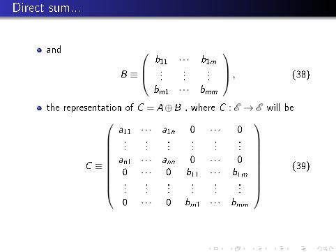
and
B ≡
b11 · · · b1m...
......
bm1 · · · bmm
, (38)
the representation of C = A⊕B , where C : E → E will be
C ≡
a11 · · · a1n 0 · · · 0...
......
......
...an1 · · · ann 0 · · · 00 · · · 0 b11 · · · b1m...
......
......
...0 · · · 0 bm1 · · · bmm
(39)

Direct Sum...
In a shorthand notation, one can write Eq. 39 as
C ≡(
A O
OT B
), (40)
where O denotes a n×m dimensional null matrix.

Direct/Tensor Product
The direct (or tensor) product space of E1 and E2 is denoted as
E = E1⊗E2, (41)
and is an nm dimensional space with the ordered basis{|ai 〉⊗ |bj〉, i = 1, . . . ,n; j = 1, . . . ,m}.Various notations used to depict the direct product basis are
|ai 〉⊗ |bj〉= |ai 〉|bj〉= |aibj〉. (42)
Similar to direct sum, one can have the direct product of twovectors, as well as two operators belonging to state spaces E1and E2 .
Let us consider two kets |v〉 ∈ E1 and |u〉 ∈ E2, de�ned in Eqs.34 and 35.

Direct product of vectors
The direct product of these two kets |w〉= |v〉⊗ |u〉 is de�nedas
|w〉= |v〉⊗ |u〉=n
∑i=1
m
∑j=1
viuj |aibj〉.
For the chosen ordered basis, the representation of |w〉 is
|w〉 ≡
v1u1...
v1umv2u1...
v2um...
vnu1...
vnum
(43)

Direct product of operators
Let us again consider linear operators A : E1→ E1 andB : E2→ E2, whose representations with respect to the givenordered basis are given by Eqs. 37 and 38.
The matrix elements of A and B are given by Aij = 〈ai |A|aj〉and Bkl = 〈bk |B|bl 〉Let us compute the matrix elements of the operatorC : E → E which is the direct product of A and B
C = A⊗B.
So that
Cik;jl = 〈aibk |A⊗B|ajbl 〉= 〈ai |A|aj〉〈bk |B|bl 〉= AijBkl . (44)

Direct product of operators
Assuming the ordered basis to be the same as consideredearlier for direct product of kets{|a1b1〉, . . . , |a1bm〉, |a2b1〉, . . . , |a2bm〉, . . . , |anb1〉, . . . , |anbm〉}We obtain the following matrix representation of C
C =
a11B · · · a1nB...
......
an1B · · · annB
, (45)
where aijB is the matrix obtained by multiplying each elementof the B matrix by aij
aijB =
aijb11 · · · aijb1m...
......
aijbm1 · · · aijbmm
. (46)

An Example of a Direct Product of Matrices
Let us illustrate the procedure of computing the direct productby considering an example involving 2×2 matrices.
Let n = m = 2, so that
A =
(a11 a12a21 a22
)B =
(b11 b12b21 b22
)So that C = A⊗B is given by
C =
a11b11 a11b12 a12b11 a12b12a11b21 a11b22 a12b21 a12b22a21b11 a21b12 a22b11 a22b12a21b21 a21b22 a22b21 a22b22
.

Addition of Angular Momenta
Suppose we have two distinct angular momenta J1 and J2,which may belong to two di�erent particles of a given system
Or may correspond to two di�erent types of angular momenta(say L and S) of the same particle
Let J1 and J2 belong to state spaces E1 and E2
Then the total angular momentum J obtained by adding J1and J2 will be symbolically denoted as J = J1 +J2
But, as we know that E1 and E2 are di�erent spaces withdi�erent dimensions, in general.
Therefore, we cannot simply add quantities belonging todi�erent state spaces

Addition of Angular Momenta...
As a matter of fact J belongs to the direct product spaceE = E1⊗E2.
We will show that the mathematically rigorous manner ofadding the two angular momenta is
J = J1⊗ I2 + I1⊗J2, (47)
where I1 ∈ E1 and I2 ∈ E2 are the identity operators.
Let us consider a rotation by an angle φ about an axis orientedalong the direction n.
Because J is the angular momentum operator in the directproduct space E = E1⊗E2, therefore it must generaterotations in that space
U(E )R = e−
ihJ·nφ . (48)

Addition of angular momenta...
Similarly, J1 and J2 are generators of rotations in spaces E1and E2 , as a result of which
U(E1)R = e−
ihJ1·nφ
U(E2)R = e−
ihJ2·nφ .
(49)
Because, E = E1⊗E2, therefore
U(E )R = U
(E1)R ⊗U
(E2)R , (50)
which implies that
e−ihJ·nφ = e−
ihJ1·nφ ⊗ e−
ihJ2·nφ (51)

Addition of angular momenta...
The RHS of the previous equation (Eq. 51) can be rewritten as
e−ihJ1·nφ ⊗ e−
ihJ2·nφ = (e−
ih
(J1⊗I2)·nφ )(e−ih
(I1⊗J2)·nφ )
= e−ih
(J1⊗12+I1⊗J2)·nφ
The last step above was possible because J1 and J2 commutewith each other, as they are in di�erent spaces. This, onsubstitution in Eq. 51 leads to
e−ihJ·nφ = e−
ih
(J1⊗I2+I1⊗J2)·nφ . (52)
On comparing the two sides, we obtain the desired result ofEq. 47
J = J1⊗ I2 + I1⊗J2.
As mentioned earlier, this result is often written in an informalmanner as a simple addition of J1 and J2 operators
J = J1 +J2. (53)

Addition of angular momenta...
Because [J1,J2] = 0, therefore, it is easy to prove that J2 andvarious components Ji satisfy the same commutation relationssatis�ed by J21 , J1i , J
22 , and J2i[
J2,Ji]
= 0[Ji ,Jj ] = i hεijkJk
(54)
Eq. 54 implies that there exists a basis |jm〉 which are thecommon eigenvectors of J2 and Jz
J2|jm〉= h2j(j +1) | jm〉Jz | jm〉= mh | jm〉
(55)
But it is easy to see
[J21 ,Jz ] = [J22 ,Jz ] = [J2,J21 ] = [J2,J22 ] = 0 (56)
This means that |jm〉 states must also be eigenvectors of J21and J22 operators, in addition J2, and Jz
J21 |jm〉= j1 (j1 +1) h2 | jm〉J22 |jm〉= j2 (j2 +1) h2 |jm〉 . (57)

Addition of Angular Momenta...
Therefore, we adopt the notation
| jm〉 → |j1j2jm〉, (58)
which indicates that these states are eigenvectors of operatorsof J21 , J
22 , J
2, and Jz .
Clearly, states |j1j2jm〉 ∈ E , which is a direct product space
But, direct product states |j1j2m1m2〉= |j1m1〉⊗ |j2m2〉 alsobelong to E
Therefore, the two sets of states must be related to each otherby a unitary transformation, because both form orthonormalsets, and span the same state space E
〈j ′1j ′2j ′m′|j1j2jm〉= δj ′1j1δj ′2j2
δj ′jδm′m
〈j ′1j ′2m′1m′2|j1j2m1m2〉= δj ′1j1δj ′2j2
δm′1m1δm′2m2
(59)

Clebsch-Gordon Coe�cients
To establish the connection between the states |j1j2jm〉 and|j1j2m1m2〉, we make use of the resolution of identity for �xedvalues of j1 and j2
I =j1
∑m1=−j1
j2
∑m2=−j2
|j1j2m1m2〉〈j1j2m1m2|, (60)
and apply it on the state |j1j2jm〉
|j1j2jm〉= I |j1j2jm〉= ∑
m1,m2
|j1j2m1m2〉〈j1j2m1m2|j1j2jm〉. (61)
From Eq. 61, it is obvious that the two sets of states areconnected by expansion coe�cients 〈j1j2m1m2|j1j2jm〉, calledClebsch-Gordon coe�cients
Next, we will study their properties, and develop approachesfor computing them.

Clebsch-Gordon Coe�cients...
Let us apply Jz = J1z +J2z operator on both the sides of Eq.61
Jz |j1j2jm〉= ∑m1,m2
(J1z +J2z)|j1j2m1m2〉〈j1j2m1m2|j1j2jm〉
This leads to
mh|j1j2jm〉= ∑m1,m2
(m1 +m2)h|j1j2m1m2〉〈j1j2m1m2|j1j2jm〉.
Taking the inner product of this equation with |j1j2m′1m′2〉 onboth the sides, and making use of the orthonormality relations(Eq. 59) we obtain
m〈j1j2m′1m′2|j1j2jm〉= (m′1 +m′2)〈j1j2m′1m′2|j1j2jm〉=⇒ m〈j1j2m1m2|j1j2jm〉= (m1 +m2)〈j1j2m1m2|j1j2jm〉

Clebsch-Gordon Coe�cients...
Leading to
(m−m1−m2)〈j1j2m1m2|j1j2jm〉= 0.
Clearly 〈j1j2m1m2|j1j2jm〉 6= 0, only if
m = m1 +m2. (62)
This formula is called �conservation of m� or �m selection rule�
This implies that only those Clebsch-Gordon coe�cients(CGCs) 〈j1j2m1m2|j1j2jm〉 will be non-vanishing for whichm = m1 +m2

Recursion Relations of Clebsch-Gordon Coe�cients
Next, we apply J+ and J− operators on Eq. 61 to deriveimportant recursions relations involving CGCs.
Note that hereJ± = J1±+J2±. (63)
With this
J±|j1j2jm〉= ∑m1,m2
(J1±+J2±)|j1j2m1m2〉〈j1j2m1m2|j1j2jm〉.
(64)
But, using Eqs. 13 , we obtain
J±|j1j2jm〉=√
(j∓m)(j±m+1)h | j1j2jm±1〉
(J1±+J2±)|j1j2m1m2〉=√
(j1∓m1)(j1±m1 +1)h|j1j2m1±1m2〉
+√
(j2∓m2)(j2±m2 +1)h|j1j2m1m2±1〉(65)

CGC Recursion Relations
Substituting Eqs. 65 in Eq. 64, we obtain√(j∓m)(j±m+1)h | j1j2jm±1〉
= ∑m1,m2
{√(j1∓m1)(j1±m1 +1)h|j1j2m1±1m2〉
+√
(j2∓m2)(j2±m2 +1)h|j1j2m1m2±1〉}〈j1j2m1m2|j1j2jm〉
(66)
We take the inner product of Eq. 66 with |j1j2m′1m′2〉, and usethe orthonormality relations of Eq. 59 to obtain√
(j∓m)(j±m+1)〈j1j2m′1m′2 | j1j2jm±1〉= ∑m1,m2
{√(j1∓m1)(j1±m1 +1)δm′1m1±1δm′2m2
+√
(j2∓m2)(j2±m2 +1)δm′1m1δm′2m2±1
}〈j1j2m1m2|j1j2jm〉,
which leads to√(j∓m)(j±m+1)〈j1j2m′1m′2 | j1j2jm±1〉
=√
(j1∓m′1 +1))(j1±m′1)〈j1j2m′1∓1m2|j1j2jm〉+√
(j2∓m′2 +1))(j2±m′2)〈j1j2m1m′2∓1|j1j2jm〉

CGC Recursion Relations
Next, we just replace m′1 and m′2 by m1 and m2, respectively,to obtain the �nal expression for the desired recursion relation√
(j∓m)(j±m+1)〈j1j2m1m2 | j1j2jm±1〉=√
(j1±m1)(j1∓m1 +1)〈j1j2m1∓1m2 | j1j2jm〉+√
(j2±m2)(j2∓m2 +1)〈j1j2m1m2∓1 | j1j2jm〉(67)

Calculating CGCs using Recursion Relations
Using recursion relation of Eq. 67, one can compute, for agiven set of j1, j2, and j , all non-vanishing CGCs, in terms ofjust one of them.
Let us choose maximum allowed values for m1 and m:m1 = j1, m = j
And let m2 = j− j1−1
Substituting these in Eq. 67 with the lower sign, we obtain√(j + j)(j− j +1)〈j1j2j1j− j1−1 | j1j2jj−1〉
=√
(j1− j1)(j1 + j1 +1)〈j1j2j1 +1j− j1−1 | j1j2jj〉+√
(j2− (j− j1−1))(j2 + j− j1−1+1)〈j1j2j1j− j1−1+1 | j1j2jj〉

Calculations of CGCs...
We note that the �rst term on the RHS of the previousequation vanishes, as a result of which we obtain
〈j1j2j1j− j1−1 | j1j2jj−1〉=√
(j1+j2+1−j)(j+j2−j1)2j
〈j1j2j1j− j1 | j1j2jj〉(68)
From Eq. 68 we can compute the CGC〈j1j2j1j− j1−1 | j1j2jj−1〉, provided the value of〈j1j2j1j− j1 | j1j2jj〉 is knownLet us again use the recursion relations of Eq. 67, but usingthe upper sign, and m1 = j1, m = j−1, and m2 = j− j1√
(j− (j−1))(j + (j−1) +1)〈j1j2j1j− j1 | j1j2j(j−1) +1〉=√
(j1 + j1)(j1− j1 +1)〈j1j2j1−1j− j1 | j1j2jj−1〉+√
(j2 + j− j1)(j2− (j− j1) +1)〈j1j2j1j− j1−1 | j1j2jj−1〉

Calculations of CGCs...
This simpli�es to
√2j 〈j1j2j1j− j1 | j1j2jj〉
=√2j1 〈j1j2j1−1j− j1 | j1j2jj−1〉
+√
(j2 + j− j1)(j1 + j2− j +1)〈j1j2j1j− j1−1 | j1j2jj−1〉 ,
leading to the �nal form
〈j1j2j1−1j− j1 | j1j2j−1〉=√
jj1〈j1j2j1j− j1 | j1j2jj〉
−√
(j2+j−j1)(j1+j2−j+1)2j1
〈j1j2j1j− j1−1 | j1j2jj−1〉 .(69)
Thus Eq. 69 allows us to compute the CGC〈j1j2j1−1j− j1 | j1j2j−1〉 if we know the values of〈j1j2j1j− j1 | j1j2jj〉 and 〈j1j2j1j− j1−1 | j1j2jj−1〉.Thus, using the recursion relations (Eq. 67) we can computeall the CGCs, provided we know the value of〈j1j2j1j− j1 | j1j2jj〉.

Triangular Inequality of CGCs
Let us derive another important selection rule for CGCs, whichallows us to compute all allowed values of j , for the givenvalues of j1 and j2.
Let us consider the CGC 〈j1j2j1j− j1 | j1j2jj〉Because j− j1 is a possible value of m2, therefore, it mustsatisfy
−j2 ≤ j− j1 ≤ j2,
from which we obtain
j1− j2 ≤ j ≤ j1 + j2 (70)
Similarly, if we consider the CGC 〈j1j2j− j2j2 | j1j2jj〉, we have
−j1 ≤ j− j2 ≤ j1,
leading toj2− j1 ≤ j ≤ j1 + j2. (71)

Triangular Inequality...
We can combine the results of Eqs. 70 and 71 in a singleinequality
|j1− j2| ≤ j ≤ j1 + j2, (72)
which is the famous triangular inequality.
Triangular inequality is nothing but a selection rule for CGCs,in addition to the �m selection rule� derived earlier.
If for a given pair of values of j1 and j2, j does not satisfytriangular inequality, the corresponding CGC will surely vanish.

Orthonormality Conditions of CGCs
Next we derive two orthonormality conditions satis�ed by theCGCs
They are quite important, although both of them can bederived quite easily using the �resolution of identity�.
We know from Eq. 59 that
〈j1j2j ′m′|j1j2jm〉= δj ′jδm′m.
We apply the resolution of identity
∑m1,m2|j1j2m1m2〉〈j1j2m1m2|= I on the left hand side of the
equation above to obtain
∑m1,m2
〈j1j2j ′m′|j1j2m1m2〉〈j1j2m1m2|j1j2jm〉= δj ′jδm′m
Assuming that the CGCs are real, i.e.,
〈j1j2j ′m′|j1j2m1m2〉= 〈j1j2m1m2|j1j2j ′m′〉

Orthonormality of CGCs...
Using this in the previous equation, we obtain the �rstorthonormality relation of the CGCs
∑m1,m2
〈j1j2m1m2|j1j2jm〉〈j1j2m1m2|j1j2j ′m′〉= δj ′jδm′m. (73)
Next, we derive the second orthonormality relation startingwith (Eq. 59)
〈j1j2m′1m′2|j1j2m1m2〉= δm′1m1δm′2m2
We insert the resolution of identity ∑j ,m |j1j2jm〉〈j1j2jm|= I onthe left to obtain
∑j ,m
〈j1j2m′1m′2|j1j2jm〉〈j1j2jm|j1j2m1m2〉= δm′1m1δm′2m2
.
Again using the reality of CGCs, we obtain our �nalorthonormality relation for CGCs
∑j ,m
〈j1j2m′1m′2|j1j2jm〉〈j2m1m2|jj2jm〉= δm′1m1δm′2m2
. (74)

Orthonormality of CGCs...
From Eqs. 73 and 74 it is obvious that CGCs form a unitarymatrix
Orthonormality condition of Eq. 73 and recursion relations(Eq. 67) are used to compute the CGCs 〈j1j2j1j− j1 | j1j2jj〉which by convention are assumed to be real and positive.
Rest of the CGCs can be obtained by further applications ofthe recursion relations, as will be demonstrated in the tutorialproblems.

Clebsch-Gordon Series
From the previous discussion it is easy to deduce that thenumber of direct product (or uncoupled) basis states|j1j2m1m2〉 ∈ E = E1⊗E2 is identical to the number of coupledstates |j1j2jm〉, which also belong to E
The number of direct product basis states is easy to count(2j1 +1)(2j2 +1). You will get the same number in thecoupled representation also (try it yourself).
This is because the two sets of states are connected by aunitary transformation whose matrix elements are CGCs
There are several consequences of this, which we explore next
The resolution of identity in the two basis sets must beidentical, which means
j1
∑m1=−j1
j2
∑m2=−j2
|j1j2m1m2〉〈j1j2m1m2|=j1+j2
∑j=|j1−j2|
j
∑m=−j
|j1j2jm〉〈j1j2jm|.
(75)

Clebsch-Gordon Series...
If we examine the RHS of Eq. 75 carefully, we realize that eachone of the kets |j1j2jm〉 belongs to a 2j +1 dimensional space.
And di�erent values of j correspond to a di�erent space, whichis a subspace of E .
As a result, the sum on the RHS of Eq. 75 is actually a directsum, i.e.,
∑j1+j2j=|j1−j2|∑
jm=−j |j1j2jm〉〈j1j2jm|
= ∑|j1−j2|m=−|j1−j2| |j1j2|j1− j2|m〉〈j1j2|j1− j2|m|
⊕∑|j1−j2|+1
m=−|j1−j2|−1 |j1j2|j1− j2|+1m〉〈j1j2|j1− j2|+1m|⊕· · ·⊕∑
j1+j2m=−(j1+j2) |j1j2j1 + j2m〉〈j1j2j1 + j2m|
(76)

Clebsch-Gordon Series...
Each term in the direct sum of Eq. 76 corresponds toresolution of identity in that subspace
If we adopt the notation
j
∑m=−j
|j1j2jm〉〈j1j2jm|= Ij , (77)
then the Eq. 76 can be written as
j1+j2
∑j=|j1−j2|
j
∑m=−j
|j1j2jm〉〈j1j2jm|= I|j1−j2|⊕ I|j1−j2|+1⊕
·· ·⊕ Ij1+j2−1⊕ Ij1+j2 . (78)

Clebsch-Gordon Series...
Similarly, we can write the identity of the uncoupledrepresentation (see the LHS of Eq. 75) as
∑j1m1=−j1 ∑
j2m2=−j2 |j1j2m1m2〉〈j1j2m1m2|
=(
∑j1m1=−j1 |j1m1〉〈j1m1|
)⊗(
∑j2m2=−j2 |j2m2〉〈j2m2|
)= Ij1⊗ Ij2
(79)
Finally, by combining Eqs. 75, 78, and 79, we have the result
Ij1⊗ Ij2 = I|j1−j2|⊕ I|j1−j2|+1⊕·· ·⊕ Ij1+j2−1⊕ Ij1+j2 . (80)
Clebsch-Gordon Series...
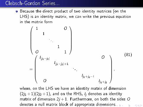
Because the direct product of two identity matrices (on theLHS) is an identity matrix, we can write the previous equationin the matrix form
1 O
1. . .
1O 1
=
I|j1−j2| O
I|j1−j2|+1
. . .
Ij1+j2−1O Ij1+j2
,
(81)
where, on the LHS we have an identity matrix of dimension(2j1 +1)(2j2 +1), and on the RHS, Ij denotes an identitymatrix of dimension 2j +1. Furthermore, on both the sides Odenotes a null matrix block of appropriate dimensions.

Clebsch-Gordon Series...
A similar result holds for the rotation matrices in the two bases
D(j1)(R)⊗D(j2)(R) = D |j1−j2|(R)⊕D |j1−j2|+1(R)⊕·· ·⊕D j1+j2−1(R)⊕D j1+j2(R). (82)
The RHS of the previous equation implies a block-diagonalnature of the rotation matrix in the coupled basis, which canalso be expressed in the matrix form similar to the case ofidentity matrix (Eq. 81)
D(j1)(R)⊗D(j2)(R) =D |j1−j2| O
D |j1−j2|+1
. . .
D j1+j2−1
O D j1+j2
(83)

Clebsch-Gordon Series....
As a matter of fact, the main reason behind the validity ofresults such as Eqs. 80 and 82 is that the direct product spaceEj1⊗Ej2 is a direct sum of the corresponding smaller subspaces
Ej1⊗Ej2 = E|j1−j2|⊕E|j1−j2|+1⊕·· ·⊕Ej1+j2−1⊕Ej1+j2 . (84)

Examples of Block-diagonal Matrices
We give examples of a couple of block-diagonal matrices Aand B below, and how they can be written as direct sums
A =
1 2 0 03 4 0 00 0 5 60 0 7 8
=
(1 23 4
)⊕(
5 67 8
)= A1⊕A2
with
A1 =
(1 23 4
)and A2 =
(5 67 8
).
This means that the operator A is block-diagonal w.r.t. to thechosen basis in the original space E , which can be written asthe direct sum of two 2-dimensional spaces E1 and E2
E = E1⊕E2.

Examples of Block-diagonal Matrices...
Let B be a 5×5 matrix
B =
1 2 3 0 04 5 6 0 07 8 9 0 00 0 0 1 −10 0 0 3 −2
=
1 2 34 5 67 8 9
⊕( 1 −13 −2
)= B1⊕B2
Here clearly the 5-dimensional space E can be written as a directsum of a 3-dimensional subspace E1 and a 2-dimensional subspaceE2
E = E1⊕E2
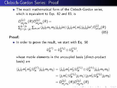
Clebsch-Gordon Series: Proof
The exact mathematical form of the Clebsch-Gordon series,which is equivalent to Eqs. 82 and 83, is
D(j1)m′1m1
(R)D(j2)m′2m2
(R) =
∑j1+j2j=|j1−j2|∑m,m′〈j1j2m1m2|j1j2jm〉〈j1j2m′1m′2|j1j2jm′〉D
(j)m′m(R)
(85)
Proof:
In order to prove the result, we start with Eq. 50
U(E )R = U
(E1)R ⊗U
(E2)R ,
whose matrix elements in the uncoupled basis (direct-productbasis) are
〈j1j2m′1m′2|U(E )R |j1j2m1m2〉= 〈j1j2m′1m′2|U
(E1)R ⊗U
(E2)R |j1j2m1m2〉
= 〈j1m′1|U(E1)R |j1m1〉〈j2m′2|U
(E2)R |j2m2〉
= D(j1)m′1m1
(R)D(j2)m′2m2
(R)

Clebsch-Gordon Series: Proof...
Using the resolution of identity in the coupled basis
∑jm |j1j2jm〉〈j1j2jm|= I on the LHS of the previous equationtwo times, and interchanging LHS and RHS, we obtain
D(j1)m′1m1
(R)D(j2)m′2m2
(R) =
∑j ,j ′,m,m′〈j1j2m′1m′2|j1j2j ′m′〉〈j1j2j ′m′|U(E )R |j1j2jm〉〈j1j2jm|j1j2m1m2〉
On using the reality of CGCs〈j1j2jm|j1j2m1m2〉= 〈j1j2m1m2|j1j2jm〉, and
〈j1j2j ′m′|U(E )R |j1j2jm〉= δj ′jD
(j)m′m(R),
we obtain the desired result
D(j1)m′1m1
(R)D(j2)m′2m2
(R) =
∑j1+j2j=|j1−j2|∑m,m′〈j1j2m1m2|j1j2jm〉〈j1j2m′1m′2|j1j2jm′〉D
(j)m′m(R)

Tensor Operators
We will �rst discuss vector operators, and then generalize thediscussion to de�ne the tensor operators.
Let us assume that there is an operator ~A, called a vectoroperator, because its expectation value rotates as per rules oftransformation of a vector, under an active rotation R .
If the system is in state |ψ〉 we know under the rotation it willtransform into |ψ ′〉 as
|ψ ′〉= UR |ψ〉
If e is an arbitrary unit vector, then clearly ~A.e is a scalar andhence its value will be invariant under the rotation
〈ψ|~A.e|ψ〉= 〈ψ ′|~A.e ′|ψ ′〉
〈ψ ′|UR~A.eU†
R |ψ′〉= 〈ψ ′|~A.e ′|ψ ′〉
UR~A.eU†
R =~A.e ′ (86)

An example of an operator of the form ~A.e
As an example, let us consider
~A = ~σ = σx i + σy j + σz k
e =1√3i +
1√3j +
1√3k ,
then clearly
~A.e =1√3
(σx + σy + σz)
~A.e =1√3
(1 1− i
1+ i −1
)

Tensor Operator(contd.)
e transforms into e ′ after the rotation. But, in a Cartesianbasis
e ′i = ∑j
Rij ej (87)
Upon substituting this above, we obtain
∑k
URAkU†R ek = ∑
i
Ai e′i
∑k
URAkU†R ek = ∑
i∑j
AiRij ej
Comparing coe�cients of ej on both the sides, we have
URAjU†R = ∑
i
AiRij (88)
Let us consider an in�nitesimal rotation about an axis n, by anangle. Then, to the �rst order
UR = e−i(~J.n)ε
h ≈ I − i(~J.n)ε
h(89)
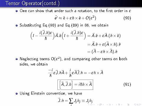
Tensor Operator(contd.)
One can show that under such a rotation, to the �rst order in ε
e ′ ≈ e + ε n× e +O(ε2) (90)
Substituting Eq.(90) and Eq.(89) in 86, we obtain(I − i(~J.n)ε
h
)~A.e(I +
i(~J.n)ε
h
)= ~A.e + ε~A.(n× e)
= ~A.e + ε(~A× n).e
= (~A− ε n×~A).e
Neglecting terms O(ε2), and comparing other terms on bothsides, we obtain
−ih
ε~J.n~A+i
hε~A~J.n =−ε n×~A[
~A,~J.n]
= i hn×~A (91)
Using Einstein convention, we have
~J.n = ∑j
Jj nj ≡ Jj nj

Tensor Operator(contd.)
Also,(n×A)i = εijk njAk
On substituting these above for the i-th component of Eq.(91), we obtain
[Ai ,Jj ] = i hεijkAk (92)
Note that this is a very profound general relation satis�ed by avector operator ~A
Unlike Eq. 88, this relation (Eq. 92) does not depend on thenature of rotation (rotation axis, or the angle of rotation) inany way.
It just involves commutation relations of various Cartesiancomponents of ~A with Cartesian components of the angularmomentum operator

Tensor Operators: De�nition
Next we de�ne a tensor operator as a generalization of avector operator.
We saw that a vector operator ~A transforms according toEq.(88) under a rotation.
We de�ne a spherical tensor operator T qk
(q =−k ,−k +1, . . . ,k−1,k) of rank k as the operator whichtransforms according to the rule
URTqkU†R =
k
∑q′=−k
Tq′
kD
(k)q′q (R) (93)

Tensor Operator(contd.)
According to this de�nition, an object of rank k = 1, is aspherical vector. Let us see how Ym
l (θ ,φ) transform for l = 1.We saw earlier
Yml (θ
′,φ ′) =l
∑m′=−l
Ym′
l (θ ,φ)D(l)m′,m, (94)
where Yml (θ ′,φ ′) is the same function with respect to the
rotated coordinate system. Noting that
URYml (θ ,φ)U†
R = Yml (θ
′,φ ′)
we �nd that Eq.(93) and Eq.(94) have the same form. ThusY lm's are tensor operators of rank l . Coming back to the case
of l = 1, we have
Y ±11 (θ ,φ) =∓√
3
8πe±iφ sinθ
=∓√
3
8π
(sinθ cosφ ± i sinθ sinφ
)

Tensor Operator(contd.)
Which can be expressed in terms of Cartesian coordinates
Y ±11 (θ ,φ) =∓√
3
8π
(x± iy)
r
Y 01 (θ ,φ) =
√3
4πcosθ =
√3
4π
z
r
(95)
So for this case Eq.(94) yields(− x ′+ iy ′√
2,z ′,
x ′− iy ′√2
)=(− x + iy√
2,z ,
x− iy√2
)D
(1)(R) (96)
Using this, we can de�ne the components of a spherical tensor,when the Cartesian components of a vector operator are given
T±11 =∓Ax ± iAy√2
T 01 = Az
(97)

Commutation Relations
For an in�nitesimal rotation of angle ε , about an axis alongthe direction n, we have from Eq.(93)
(I − i
h~J.nε
)T
qk
(I +
i
h~J.nε
)=
k
∑q′=−k
Tq′
k〈kq′|I − i
h~J.nε|kq〉
Above we used the fact that D(k)q′,q(R) = 〈kq′|UR |kq〉, and for
an in�nitesimal rotation UR ≈ I − ih~J.nε
⇒ Tqk
+i
h[T q
k,~J.n]ε +O(ε
2) = Tqk− i
hε ∑q′=−k
Tq′
k〈kq′|~J.n|kq〉
⇒ [n.~J,T qk
] =k
∑q′=−k
Tq′
k〈kq′|n.~J|kq〉 (98)

Commutation Relations(contd.)
Taking n = k , we obtain above
[Jz ,Tqk
] = qhTqk
(99)
and n = n± = i ± i j , so that
~J.n = J±
and using the fact that
J±|kq〉= h√
(k∓q)(k±q+1)|kq±1〉
we obtain
[J±,Tqk
] = h√
(k∓q)(k±q+1)T q±1k
(100)
Eq.(99) and Eq.(100) are fundamental commutation relationsof tensor operators.
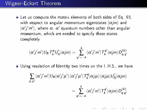
Wigner-Eckart Theorem
Let us compute the matrix elements of both sides of Eq. 93,with respect to angular momentum eigenstates |α jm〉 and|α ′j ′m′〉, where α , α ′ quantum numbers other than angularmomentum, which are needed to specify these statescompletely
〈α ′j ′m′|URTqkU†R |α jm〉=
k
∑q′=−k
〈α ′j ′m′|T q′
k|α jm〉D(k)
q,q′
Using resolution of Identity two times on the L.H.S., we have
∑µ,µ ′〈α ′j ′m′|UR |α ′j ′µ ′〉〈α ′j ′µ ′|T q
k|α jµ〉〈α jµ|U†
R |α jm〉
=k
∑q′=−k
〈α ′j ′m′|T q′
k|α jm〉D(k)
q,q′

Wigner-Eckart Theorem(contd.)
but
〈α ′j ′m′|UR |α ′j ′µ ′〉= D(j ′)m′,µ ′(R)
〈α jµ|U†R |α jm〉= D
(j)∗m,µ (R)
we obtain
∑µ,µ ′
D(j ′)m′,µ ′(R)〈α ′j ′µ ′|T q
k|α jµ〉D(j)∗
m,µ (R)
=k
∑q′=−k
〈α ′j ′m′|T q′
k|α jm〉D(k)
q,q′
(101)
we can recast C-G series of Eq.(85) as (proof is given inproblem 1 of tutorial sheet # 2)
∑µ,µ ′
D(j ′)m′,µ ′(R)〈jkmq|jkj ′µ ′〉D(j)∗
m,µ (R)
=k
∑q′=−k
〈jkmq′|jkj ′m′〉D(k)q,q′
(102)

Wigner-Eckart Theorem(contd.)
Eq.(101) can be seen as a linear homogeneous equation for
〈α ′j ′m′|T q′
k|α jm〉 and Eq.(102) has the same coe�cient
except that it has unknowns 〈jkmq′|jkj ′m′〉.Thus, the solutions of two equations, must be proportional toeach other. Thus
〈α ′j ′m′|T qk|α jm〉= 〈jkmq|jkj ′m′〉
〈α ′j ′||Tk ||α j〉,(103)
we also changed q′→ q.
where the proportionality constant 〈α ′j ′||Tk ||α j〉 is called thereduced Matrix element.
They depend only on α , α ′, j , j ′, and not on m, m′, and q
because that dependence is contained in the C-G-C〈jkmq|jkj ′m′〉 Eq.(103) is called the Wigner-Eckart theorem.
Wigner-Eckart Theorem(contd.)
The importance of Wigner-Eckart theorem lies in the fact thatthe required matrix element is written as a product of C-G-Cwhich contains the symmetry related information, and reducedmatrix element which contains information about otherproperties of the system.

Selection Rules
From the CGC involved in the Wigner-Eckart theoremEq.(103), we get two important selection rules whichdetermine whether a given matrix element is zero, based juston the symmetry. We know that the CGC 〈jkmq|jkj ′m′〉 is nonzero only if
1 m selection rule is valid, i.e.,
m′ = m+q
⇒ q = m′−m (104)
2 Triangular Identity is valid, i.e.,
|j−k| ≤ j ′ ≤ j +k
But triangular identity of numbers holds for all three numbers
⇒ |j− j ′| ≤ k ≤ j + j ′ (105)
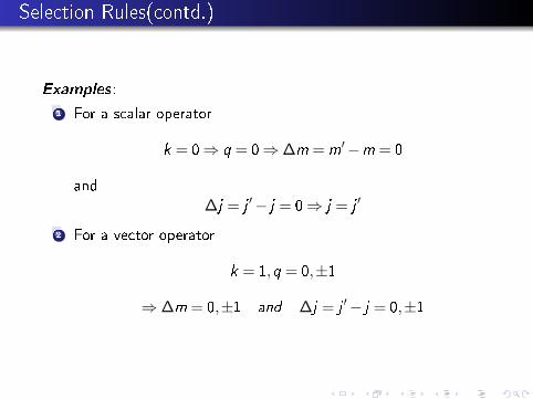
Selection Rules(contd.)
Examples:
1 For a scalar operator
k = 0⇒ q = 0⇒∆m = m′−m = 0
and∆j = j ′− j = 0⇒ j = j ′
2 For a vector operator
k = 1,q = 0,±1
⇒∆m = 0,±1 and ∆j = j ′− j = 0,±1

Projection Theorem
For a vector operator ~A, with spherical components Aq1 or Aq
for short,
〈α ′jm′|Aq|α jm〉=〈α ′jm|~J.~A|α jm〉
h2j(j +1)×〈jm′|Jq|jm〉
Proof: We have
~J.~A = JxAx +JyAy +JzAz
=1
2(Jx + iJy )(Ax − iAy )
+1
2(Jx − iJy )(Ax + iAy ) +JzAz
=−J+1A−1−J−1A+1 +J0A0
where
A±1 =∓ 1√2
(Ax ± iAy )
A0 = Az

Projection Theorem(contd.)
J±1 =∓ 1√2
(Jx ± iJy ) =∓ 1√2J±
J0 = Jz
with this
〈α ′jm|~J.~A|α jm〉= 〈α ′jm|J0A0−J+1A−1−J−1A+1|α jm〉= mh〈α ′jm|A0|α jm〉
+h√2
√(j +m)(j−m+1)〈α ′jm−1|A−1|α jm〉
− h√2
√(j−m)(j +m+1)〈α ′jm+1|A+1|α jm〉

Projection Theorem(contd.)
But from Wigner-Eckart theorem
〈α ′jm|A0|α jm〉 ∝ 〈α ′jm|A+1|α jm〉
∝ 〈α ′jm|A−1|α jm〉 ∝ 〈α ′j ||~A||α j〉
where 〈α ′j ||~A|α j〉 is the reduced Matrix element of ~A,independent of m and q. Thus,
〈α ′jm|~J.~A|α jm〉= C (j ,m)〈α ′j ||~A||α j〉
where C (j ,m) is a constant which depends on j and m, and isindependent of α , α ′, and ~A.
Furthermore, C (j ,m) must be independent of m as wellbecause ~J.~A is a scalar operator, thus
〈α ′jm|~J.~A|α jm〉= C (j)〈α ′j ||~A||α j〉

Projection Theorem(contd.)
This will be valid also for ~A =~J, with α ′ = α
〈α jm|J2|α jm〉= C (j)〈α j ||~J||α j〉
but 〈α jm|J2|α jm〉= j(j +1)h2
⇒ C (j) =j(j +1)h2
〈α j ||~J||α j〉
⇒ 〈α ′jm|~J.~A|α jm〉=j(j +1)h2〈α ′j ||~A||α j〉
〈α j ||~J||α j〉(106)
using Wigner-Eckart theorem, we have
⇒ 〈α ′jm′|Aq|α jm〉= 〈j1mq|j1jm′〉〈α ′j ||~A||α j〉
and⇒ 〈α jm′|Jq|α jm〉= 〈j1mq|j1jm′〉〈α ′j ||~J||α j〉

Projection Theorem(contd.)
Taking the ratio of these two equations, we have
〈α ′j ||~A|α j〉〈α ′j ||~J|α j〉
=〈α ′jm′|Aq|α jm〉〈α jm′|Jq|α jm〉
(107)
on substituting Eq.(107) in Eq.(106) we obtained the desiredresult
〈α ′jm′|Aq|α jm〉=〈α ′jm|~J.~A|α jm〉
j(j +1)h2×〈jm′|Jq|jm〉 (108)
The importance of projection theorem is that it shows that theexpectation value of any vector operator is proportional to theexpectation value of the angular momentum operator.
This implies that any vector associated with a sphericallysymmetric quantum mechanical system will be either parallelor anti parallel to its angular momentum.