angular momentum 1 angular momentum in...
TRANSCRIPT
J. Broida UCSD Fall 2009
Phys 130B QM II
Angular Momentum
1 Angular momentum in Quantum Mechanics
As is the case with most operators in quantum mechanics, we start from the clas-sical definition and make the transition to quantum mechanical operators via thestandard substitution x → x and p → −i~∇. Be aware that I will not distinguisha classical quantity such as x from the corresponding quantum mechanical operatorx. One frequently sees a new notation such as x used to denote the operator, butfor the most part I will take it as clear from the context what is meant. I will alsogenerally use x and r interchangeably; sometimes I feel that one is preferable overthe other for clarity purposes.
Classically, angular momentum is defined by
L = r× p .
Since in QM we have[xi, pj ] = i~δij
it follows that [Li, Lj] 6= 0. To find out just what this commutation relation is, firstrecall that components of the vector cross product can be written (see the handoutSupplementary Notes on Mathematics)
(a × b)i = εijkajbk .
Here I am using a sloppy summation convention where repeated indices are summedover even if they are both in the lower position, but this is standard when it comesto angular momentum. The Levi-Civita permutation symbol has the extremelyuseful property that
εijkεklm = δilδjm − δimδjl .
Also recall the elementary commutator identities
[ab, c] = a[b, c] + [a, c]b and [a, bc] = b[a, c] + [a, b]c .
Using these results together with [xi, xj ] = [pi, pj ] = 0, we can evaluate the com-mutator as follows:
[Li, Lj] = [(r × p)i, (r × p)j ] = [εiklxkpl, εjrsxrps]
= εiklεjrs[xkpl, xrps] = εiklεjrs(xk[pl, xrps] + [xk, xrps]pl)
1
= εiklεjrs(xk[pl, xr]ps + xr[xk, ps]pl) = εiklεjrs(−i~δlrxkps + i~δksxrpl)
= −i~εiklεjlsxkps + i~εiklεjrkxrpl = +i~εiklεljsxkps − i~εjrkεkilxrpl
= i~(δijδks − δisδjk)xkps − i~(δjiδrl − δjlδri)xrpl
= i~(δijxkpk − xjpi) − i~(δijxlpl − xipj)
= i~(xipj − xjpi) .
But it is easy to see that
εijkLk = εijk(r × p)k = εijkεkrsxrps = (δirδjs − δisδjr)xrps
= xipj − xjpi
and hence we have the fundamental angular momentum commutation relation
[Li, Lj] = i~εijkLk . (1.1a)
Written out, this says that
[Lx, Ly] = i~Lz [Ly, Lz] = i~Lx [Lz, Lx] = i~Ly .
Note that these are just cyclic permutations of the indices x→ y → z → x.Now the total angular momentum squared is L2 = L · L = LiLi, and therefore
[L2, Lj] = [LiLi, Lj] = Li[Li, Lj] + [Li, Lj ]Li
= i~εijkLiLk + i~εijkLkLi .
ButεijkLkLi = εkjiLiLk = −εijkLiLk
where the first step follows by relabeling i and k, and the second step follows by theantisymmetry of the Levi-Civita symbol. This leaves us with the important relation
[L2, Lj ] = 0 . (1.1b)
Because of these commutation relations, we can simultaneously diagonalize L2
and any one (and only one) of the components of L, which by convention is takento be L3 = Lz. The construction of these eigenfunctions by solving the differentialequations is at least outined in almost every decent QM text. (The old book In-troduction to Quantum Mechanics by Pauling and Wilson has an excellent detaileddescription of the power series solution.) Here I will follow the algebraic approachthat is both simpler and lends itself to many more advanced applications. Themain reason for this is that many particles have an intrinsic angular momentum(called spin) that is without a classical analogue, but nonetheless can be describedmathematically exactly the same way as the above “orbital” angular momentum.
2
In view of this generality, from now on we will denote a general (Hermitian)angular momentum operator by J. All we know is that it obeys the commutationrelations
[Ji, Jj ] = i~εijkJk (1.2a)
and, as a consequence,[J2, Ji] = 0 . (1.2b)
Remarkably, this is all we need to compute the most useful properties of angularmomentum.
To begin with, let us define the ladder (or raising and lowering) operators
J+ = Jx + iJy
J− = (J+)† = Jx − iJy .(1.3a)
Then we also have
Jx =1
2(J+ + J−) and Jy =
1
2i(J+ − J−) . (1.3b)
Because of (1.2b), it is clear that
[J2, J±] = 0 . (1.4)
In addtion, we have
[Jz, J±] = [Jz, Jx] ± i[Jz, Jy] = i~Jy ± ~Jx
so that[Jz, J±] = ±~J± . (1.5a)
Furthermore,[Jz, J
2±] = J±[Jz, J±] + [Jz, J±]J± = ±2~J2
±
and it is easy to see inductively that
[Jz, Jk±] = ±k~Jk
± . (1.5b)
It will also be useful to note
J+J− = (Jx + iJy)(Jx − iJy) = J2x + J2
y − i[Jx, Jy]
= J2x + J2
y + ~Jz
and hence (since J2x + J2
y = J2 − J2z )
J2 = J+J− + J2z − ~Jz . (1.6a)
Similarly, it is easy to see that we also have
J2 = J−J+ + J2z + ~Jz . (1.6b)
3
Because J2 and Jz commute they may be simultaneously diagonalized, and wedenote their (un-normalized) simultaneous eigenfunctions by Y β
α where
J2Y βα = ~
2αY βα and JzY
βα = ~βY β
α .
Since Ji is Hermitian we have the general result
〈J2i 〉 = 〈ψ|J2
i ψ〉 = 〈Jiψ|Jiψ〉 = ‖Jiψ‖2 ≥ 0
and hence 〈J2〉 − 〈J2z 〉 = 〈J2
x〉+ 〈J2y 〉 ≥ 0. But J2
zYβα = ~
2β2Y βα and hence we must
haveβ2 ≤ α . (1.7)
Now we can investigate the effect of J± on these eigenfunctions. From (1.4) wehave
J2(J±Yβα ) = J±(J2Y β
α ) = ~2α(J±Y
βα )
so that J± doesn’t affect the eigenvalue of J2. On the other hand, from (1.5a) wealso have
Jz(J±Yβα ) = (J±Jz ± ~J±)Y β
α = ~(β ± 1)J±Yβα
and hence J± raises or lowers the eigenvalue ~β by one unit of ~. And in general,from (1.5b) we see that
Jz((J±)kY βα ) = (J±)k(JzY
βα ) ± k~(J±)kY β
α = ~(β ± k)(J±)kY βα
so the k-fold application of J± raises or lowers the eigenvalue of Jz by k units of ~.This shows that (J±)kY β
α is a simultaneous eigenfunction of both J2 and Jz withcorresponding eigenvalues ~
2α and ~(β ± k), and hence we can write
(J±)kY βα = Y β±k
α (1.8)
where the normalization is again unspecified.Thus, starting from a state Y β
α with a J2 eigenvalue ~2α and a Jz eigenvalue ~β,
we can repeatedly apply J+ to construct an ascending sequence of eigenstates withJz eigenvalues ~β, ~(β + 1), ~(β+ 2), . . . , all of which have the same J2 eigenvalue~
2α. Similarly, we can apply J− to construct a descending sequence ~β, ~(β − 1),~(β − 2), . . . , all of which also have the same J2 eigenvalue ~
2α. However, becauseof (1.7), both of these sequences must terminate.
Let the upper Jz eigenvalue be ~βu and the lower eigenvalue be −~βl. Thus, bydefinition,
JzYβu
α = ~βuYβu
α and JzYβlα = −~βlY
βlα (1.9a)
withJ+Y
βu
α = 0 and J−Yβlα = 0 (1.9b)
and where, by (1.7), we must have
β2u ≤ α and β2
l ≤ α .
4
By construction, there must be an integral number n of steps from −βl to βu, sothat
βl + βu = n . (1.10)
(In other words, the eigenvalues of Jz range over the n intervals −βl, −βl + 1,−βl + 2, . . . ,−βl + (βl + βu) = βu.)
Now, using (1.6b) we have
J2Y βu
α = J−J+Yβu
α + (J2z + ~Jz)Y
βu
α .
Then by (1.9b) and the definition of Y βα , this becomes
~2αY βu
α = ~2βu(βu + 1)Y βu
α
so thatα = βu(βu + 1) .
In a similar manner, using (1.6a) we have
J2Y βlα = J+J−Y
βlα + (J2
z − ~Jz)Yβlα
or~
2αY βlα = ~
2βl(βl + 1)Y βlα
so alsoα = βl(βl + 1) .
Equating both of these equations for α and recalling (1.10) we conclude that
βu = βl =n
2:= j
where j is either integral or half-integral, depending on whether n is even or odd.In either case, we finally arrive at
α = j(j + 1) (1.11)
and the eigenvalues of Jz range from −~j to ~j in integral steps of ~.We can now label the eigenvalues of Jz by ~m instead of ~β, where the integer or
half-integer m ranges from −j to j in integral steps. Thus our eigenvalue equationsmay be written
J2Y mj = j(j + 1)~2Y m
j
JzYmj = m~Y m
j .(1.12)
We say that the states Y mj are angular momentum eigenstates with angular mo-
mentum j and z-component of angular momentum m. Note that (1.9b) is nowwritten
J+Yjj = 0 and J−Y
−jj = 0 . (1.13)
5
Since (J±)† = J∓, using equations (1.6) we have
〈J±Y mj |J±Y m
j 〉 = 〈Y mj |J∓J±Y m
j 〉 = 〈Y mj |(J2 − J2
z ∓ ~Jz)Ymj 〉
= ~2[j(j + 1) −m2 ∓m]〈Y m
j |Y mj 〉
= ~2[j(j + 1) −m(m± 1)]〈Y m
j |Y mj 〉 .
We know that J±Ymj is proportional to Y m±1
j . So if we assume that the Y mj are
normalized, then this equation implies that
J±Ymj = ~
√j(j + 1) −m(m± 1)Y m±1
j . (1.14)
If we start at the top state Y jj , then by repeatedly applying J−, we can construct all
of the states Y mj . Alternatively, we could equally well start from Y −j
j and repeatedlyapply J+ to also construct the states.
Let us see if we can find a relation that defines the Y mj . Since Y j
j is defined
by J+Yjj = 0, we will only define our states up to an overall normalization factor.
Using (1.14), we have
J−Yjj = ~
√j(j + 1) − j(j − 1)Y j−1
j = ~
√2j Y j−1
j
or
Y j−1j = ~
−1 1√2jJ−Y
jj .
Next we have
(J−)2Y jj = ~
2√
2j√j(j + 1) − (j − 1)(j − 2)Y j−2
j = ~2√
(2j)2(2j − 1)Y j−2j
or
Y j−2j = ~
−2 1√(2j)(2j − 1)2
(J−)2Y jj .
And once more should do it:
(J−)3Y jj = ~
3√
(2j)(2j − 1)2√j(j + 1) − (j − 2)(j − 3)Y j−3
j
= ~3√
(2j)(2j − 1)(2)(3)(2j − 2)Y j−3j
or
Y j−3j = ~
−3 1√2j(2j − 1)(2j − 2)3!
(J−)3Y jj .
Noting that m = j − 3 so that 3! = (j −m)! and 2j − 3 = 2j − (j −m) = j +m, itis easy to see we have shown that
Y mj = ~
m−j
√(j +m)!
(2j)!(j −m)!(J−)j−mY j
j . (1.15a)
6
And an exactly analogous argument starting with Y −jj and applying J+ repeatedly
shows that we could also write
Y mj = ~
−m−j
√(j −m)!
(2j)!(j +m)!(J+)j+mY −j
j . (1.15b)
It is extremely important to realize that everything we have done up to thispoint depended only on the commutation relation (1.2a), and hence applies to bothinteger and half-integer angular momenta. While we will return in a later section todiscuss spin (including the half-integer case), for the rest of this section we restrictourselves to integer values of angular momentum, and hence we will be discussingorbital angular momentum.
The next thing we need to do is to actually construct the angular momentumwave functions Y m
l (θ, φ). (Since we are now dealing with orbital angular momen-tum, we replace j by l.) To do this, we first need to write L in spherical coordinates.One way to do this is to start from Li = (r×p)i = εijkxjpk where pk = −i~(∂/∂xk),and then use the chain rule to convert from Cartesian coordinates xi to sphericalcoordinates (r, θ, φ). Using
x = r sin θ cosφ y = r sin θ sinφ z = r cos θ
so that
r = (x2 + y2 + z2)1/2 θ = cos−1 z/r φ = tan−1 y/x
we have, for example,
∂
∂x=∂r
∂x
∂
∂r+∂θ
∂x
∂
∂θ+∂φ
∂x
∂
∂φ
=x
r
∂
∂r+
xz
r3 sin θ
∂
∂θ− y
x2cos2 φ
∂
∂φ
= sin θ cosφ∂
∂r+
cos θ cosφ
r
∂
∂θ− sinφ
r sin θ
∂
∂φ
with similar expressions for ∂/∂y and ∂/∂z. Then using terms such as
Lx = ypz − zpy = −i~(y∂
∂z− z
∂
∂y
)
we eventually arrive at
Lx = −i~(− sinφ
∂
∂θ− cot θ cosφ
∂
∂φ
)(1.16a)
Ly = −i~(
cosφ∂
∂θ− cot θ sinφ
∂
∂φ
)(1.16b)
Lz = −i~ ∂
∂φ. (1.16c)
7
However, another way is to start from the gradient in spherical coordinates (seethe section on vector calculus in the handout Supplementary Notes on Mathematics)
∇ = r∂
∂r+ θ
1
r
∂
∂θ+ φ
1
r sin θ
∂
∂φ.
Then L = r × p = −i~ r × ∇ = −i~ r (r × ∇) so that (since r, θ and φ areorthonormal)
L = −i~r[r × r
∂
∂r+ r × θ1
r
∂
∂θ+ r × φ 1
r sin θ
∂
∂φ
]
= −i~[φ∂
∂θ− θ 1
sin θ
∂
∂φ
]
If we write the unit vectors in terms of their Cartesian components (again, see thehandout on vector calculus)
θ = (cos θ cosφ, cos θ sinφ,− sin θ)
φ = (− sinφ, cosφ, 0)
then
L = −i~[x
(− sinφ
∂
∂θ− cot θ cosφ
∂
∂φ
)+ y
(cosφ
∂
∂θ− cot θ sinφ
∂
∂φ
)+ z
∂
∂φ
]
which is the same as we had in (1.16).Using these results, it is now easy to write the ladder operators L± = Lx ± iLy
in spherical coordinates:
L± = ±~e±iφ
(∂
∂θ± i cot θ
∂
∂φ
). (1.17)
To find the eigenfunctions Y ml (θ, φ), we start from the definition L+Y
ll = 0. This
yields the equation∂Y l
l
∂θ+ i cot θ
∂Y ll
∂φ= 0 .
We can solve this by the usual approach of separation of variables if we writeY l
l (θ, φ) = T (θ)F (φ). Substituting this and dividing by TF we obtain
1
T cot θ
∂T
∂θ= −i 1
F
∂F
∂φ.
Following the standard argument, the left side of this is a function of θ only, andthe right side is a function of φ only. Since varying θ won’t affect the right side,and varying φ won’t affect the left side, it must be that both sides are equal to aconstant, which I will call k. Now the φ equation becomes
dF
F= ikdφ
8
which has the solution F (φ) = eikφ (up to normalization). But Y ll is an eigenfunc-
tion of Lz = −i~(∂/∂φ) with eigenvalue l~, and hence so is F (φ) (since T (θ) justcancels out). This means that
−i~∂eikφ
∂φ= k~eikφ := l~eikφ
and therefore we must have k = l, so that (up to normalization)
Y ll = eilφT (θ) .
With k = l, the θ equation becomes
dT
T= l cot θ dθ = l
cos θ
sin θdθ = l
d sin θ
sin θ.
This is also easily integrated to yield (again, up to normalization)
T (θ) = sinl θ .
Thus, we can writeY l
l = cll(sin θ)leilφ
where cll is a normalization constant, fixed by the requirement that
∫ ∣∣Y ll
∣∣2 dΩ = 2π∣∣cll
∣∣2∫ π
0
(sin θ)2l sin θ dθ = 1 . (1.18)
I will go through all the details involved in doing this integral. You are free to skipdown to the result if you wish (equation (1.21)), but this result is also used in otherphysical applications.
First I want to prove the relation∫
sinn xdx = − 1
nsinn−1 x cosx+
n− 1
n
∫sinn−2 xdx . (1.19)
This is done as an integration by parts (remember the formula∫u dv = uv −∫
v du) letting u = sinn−1 x and dv = sinxdx so that v = − cosx and du =(n− 1) sinn−2 x cosxdx. Then (using cos2 x = 1 − sin2 x in the third line)
∫sinn xdx =
∫sinn−1 x sinxdx
= − sinn−1 x cosx+ (n− 1)
∫sinn−2 x cos2 xdx
= − sinn−1 x cosx+ (n− 1)
∫sinn−2 xdx − (n− 1)
∫sinn xdx .
Now move the last term on the right over to the left, divide by n, and the result is(1.19).
9
We need to evaluate (1.19) for the case where n = 2l+ 1. To get the final resultin the form we want, we will need the basically simple algebraic result
(2l + 1)!! =(2l + 1)!
2ll!l = 1, 2, 3, . . . (1.20)
where the double factorial is defined by
n!! = n(n− 2)(n− 4)(n− 6) · · · .
There is nothing fancy about the proof of this fact. Noting that n = 2l+1 is alwaysodd, we have
n!! = 1 · 3 · 5 · 7 · 9 · · · (n− 4) · (n− 2) · n
=1 · 2 · 3 · 4 · 5 · 6 · 7 · 8 · 9 · · · (n− 4) · (n− 3) · (n− 2) · (n− 1) · n
2 · 4 · 6 · 8 · · · (n− 3) · (n− 1)
=1 · 2 · 3 · 4 · 5 · 6 · 7 · 8 · 9 · · · (n− 4) · (n− 3) · (n− 2) · (n− 1) · n
(2 · 1)(2 · 2)(2 · 3)(2 · 4) · · · (2 · n−32 )(2 · n−1
2 )
=n!
2n−1
2 (n−12 )!
.
Substituting n = 2l+ 1 we arrive at (1.20).Now we are ready to do the integral in (1.18). Since the limits of integration
are 0 and π, the first term on the right side of (1.19) always vanishes, and we canignore it. Then we have
∫ π
0
(sinx)2l+1 dx =2l
2l+ 1
∫ π
0
(sinx)2l−1 dx
=
(2l
2l+ 1
) (2l− 2
2l− 1
) ∫ π
0
(sinx)2l−3 dx
=
(2l
2l+ 1
) (2l− 2
2l− 1
) (2l− 4
2l− 3
) ∫ π
0
(sinx)2l−5 dx
= · · · =
(2l
2l+ 1
)(2l− 2
2l− 1
) (2l − 4
2l − 3
)
× · · · ×(
2l − (2l− 2)
2l − (2l− 3)
) ∫ π
0
sinxdx
=2ll(l − 1)(l − 2) · · · (l − (l − 1))
(2l + 1)!!2
= 22ll!
(2l+ 1)!!= 2
(2ll!)2
(2l + 1)!(1.21)
10
where we used∫ π
0sinxdx = 2 and (1.20).
Using this result, (1.18) becomes
4π∣∣cll
∣∣2 (2ll!)2
(2l+ 1)!= 1
and hence
cll = (−1)l
[(2l + 1)!
4π
]1/21
2ll!(1.22)
where we included a conventional arbitrary phase factor (−1)l. Putting this alltogether, we have the top orbital angular momentum state
Y ll (θ, φ) = (−1)l
[(2l + 1)!
4π
]1/21
2ll!(sin θ)leilφ . (1.23)
To construct the rest of the states Y ml (θ, φ), we repeatedly apply L− from equa-
tion (1.17) to finally obtain
Y ml (θ, φ) = (−1)l
[(2l+ 1)!
4π
]1/21
2ll!
[(l +m)!
(2l)!(l −m)!
]1/2
× eimφ(sin θ)−m dl−m
d(cos θ)l−m(sin θ)2l . (1.24)
It’s just not worth going through this algebra also.
2 Spin
It is an experimental fact that many particles, and the electron in particular, havean intrinsic angular momentum. This was originally deduced by Goudsmit and Uh-lenbeck in their analysis of the famous sodium D line, which arises by the transitionfrom the 1s22s22p63p excited state to the ground state. What initially appears as astrong single line is slightly split in the presence of a magnetic field into two closelyspaced lines (Zeeman effect). This (and other lines in the Na spectrum) indicates adoubling of the number of states available to the valence electron.
To explain this “fine structure” of atomic spectra, Goudsmit and Uhlenbeckproposed in 1925 that the electron possesses an intrinsic angular momentum inaddition to the orbital angular momentum due to its motion about the nucleus.Since magnetic moments are the result of current loops, it was originally thoughtthat this was due to the electron spinning on its axis, and hence this intrinsic angularmomentum was called spin. However, a number of arguments can be put forth todisprove that classical model, and the result is that we must assume that spin is apurely quantum phenomena without a classical analogue.
As I show at the end of this section, the classical model says that the magneticmoment µ of a particle of charge q and mass m moving in a circle is given by
µ =q
2mcL
11
where L is the angular momentum with magnitude L = mvr. Furthermore, theenergy of such a charged particle in a magnetic field B is −µ · B. Goudsmit andUhlenbeck showed that the ratio of magnetic moment to angular momentum of theelectron was in fact twice as large as it would be for an orbital angular momentum.(This factor of 2 is explained by the relativistic Dirac theory.) And since we knowthat a state with angular momentum l is (2l + 1)-fold degenerate, the splittingimplies that the electron has an angular momentum ~/2.
From now on, we will assume that spin is described by the usual angular momen-tum theory, and hence we postulate a spin operator S and corresponding eigenstates|sms〉 such that
[Si, Sj ] = iεijkSk (2.1a)
S2|sms〉 = s(s+ 1)~2|sms〉 (2.1b)
Sz|sms〉 = ms~|sms〉 (2.1c)
S±|sms〉 = ~
√s(s+ 1) −ms(ms ± 1) |sms ± 1〉 . (2.1d)
(I am switching to the more abstract notation for the eigenstates because the statesthemselves are a rather abstract concept.) We will sometimes drop the subscript son ms if there is no danger of confusing this with the eigenvalue of Lz, which wewill also sometimes write as ml. Be sure to realize that particles can have a spin sthat is any integer multiple of 1/2, and there are particles in nature that have spin0 (e.g., the pion), spin 1/2 (e.g., the electron, neutron, proton), spin 1 (e.g., thephoton, but this is a little bit subtle), spin 3/2 (the ∆’s), spin 2 (the hypothesizedgraviton) and so forth.
Since the z component of electron spin can take only one of two values ±~/2, wewill frequently denote the corresponding orthonormal eigenstates simply by |z±〉,where |z+〉 is called the spin up state, and |z−〉 is called the spin down state.An arbitrary spin state |χ〉 is of the form
|χ〉 = c+|z+〉 + c−|z−〉 . (2.2a)
If we wish to think in terms of explicit matrix representations, then we will writethis in the form
χ = c+χ(z)+ + c−χ
(z)− . (2.2b)
Be sure to remember that the normalized states |sms〉 belong to distinct eigenvaluesof a Hermitian operator, and hence they are in fact orthonormal.
To construct the matrix representation of spin operators, we need to first choosea basis for the space of spin states. Since for the electron there are only two possiblestates for the z component, we need to pick a basis for a two-dimensional space,and the obvious choice is the standard basis
χ(z)+ =
[1
0
]and χ
(z)− =
[0
1
]. (2.3)
12
With this choice of basis, we can now construct the 2 × 2 matrix representation ofthe spin operator S.
Note that the existence of spin has now led us to describe the electron by amulti-component state vector (in this case, two components), as opposed to thescalar wave functions we used up to this point. These two-component states arefrequently called spinors.
The states χ(z)± were specifically constructed to be eigenstates of Sz (recall that
we simultaneously diagonalized J2 and Jz), and hence the matrix representationof Sz is diagonal with diagonal entries that are precisely the eigenvalues ±~/2. Inother words, we have
〈z ± |Sz|z±〉 = ±~
2
so that
Sz =~
2
[1 0
0 −1
]. (2.4)
(We are being somewhat sloppy with notation and using the same symbol Sz todenote both the operator and its matrix representation.) That the vectors definedin (2.3) are indeed eigenvectors of Sz is easy to verify:
~
2
[1 0
0 −1
] [1
0
]=
~
2
[1
0
]and
~
2
[1 0
0 −1
][0
1
]= −~
2
[0
1
].
To find the matrix representations of Sx and Sy, we use (2.1d) together withS± = Sx ± iSy so that Sx = (S+ + S−)/2 and Sy = (S+ − S−)/2i. From
S±|zms〉 = ~
√3/4 −ms(ms ± 1) |zms ± 1〉
we have
S+|z+〉 = 0 S−|z+〉 = ~|z−〉
S+|z−〉 = ~|z+〉 S−|z−〉 = 0 .
Therefore the only non-vanishing entry in S+ is 〈z + |S+|z−〉, and the only non-vanishing entry in S− is 〈z − |S−|z+〉. Thus we have
S+ = ~
[0 1
0 0
]and S− = ~
[0 0
1 0
].
Using these, it is easy to see that
Sx =~
2
[0 1
1 0
]and Sy =
~
2
[0 −ii 0
]. (2.5)
13
And from (2.4) and (2.5) it is easy to calculate S2 = S2x + S2
y + S2z to see that
S2 =3
4~
2
[1 0
0 1
]
which agrees with (2.1b).It is conventional to write S in terms of the Pauli spin matrices σ defined by
S =~
2σ
where
σx =
[0 1
1 0
]σy =
[0 −ii 0
]σz =
[1 0
0 −1
]. (2.6)
Memorize these. The Pauli matrices obey several relations that I leave to you toverify (recall that the anticommutator is defined by [a, b]+ = ab+ ba):
[σi, σj ] = 2iεijkσk (2.7a)
σiσj = iεijkσk for i 6= j (2.7b)
[σi, σj ]+ = 2Iδij (2.7c)
σiσj = Iδij + iεijkσk (2.7d)
Given three-component vectors a and b, equation (2.7d) also leads to the extremelyuseful result
(a · σ)(b · σ) = (a · b)I + i(a × b) · σ . (2.8)
We will use this later when we discuss rotations.From the standpoint of physics, what equations (2.2) say is that if we have
an electron (or any spin one-half particle) in an arbitrary spin state χ, then the
probablility is |c+|2 that a measurement of the z component of spin will result in
+~/2, and the probability is |c−|2 that the measurement will yield −~/2. We cansay this because (2.2) expresses χ as a linear superposition of eigenvectors of Sz.
But we could equally well describe χ in terms of eigenvectors of Sx. To do so,we simply diagonalize Sx and use its eigenvectors as a new set of basis vectors forour two-dimensional spin space. Thus we must solve Sxv = λv for λ and then theeigenvectors v. This is straightforward. The eigenvalue equation is (Sx −λI)v = 0,so in order to have a non-trivial solution we must have
det(Sx − λI) =
∣∣∣∣∣−λ ~/2
~/2 −λ
∣∣∣∣∣ = λ2 − ~2/4 = 0
so that λ± = ±~/2 as we should expect. To find the eigenvector corresponding toλ+ = +~/2 we solve
(Sx − λ+I)v =~
2
[−1 1
1 −1
] [a
b
]= 0
14
so that a = b and the normalized eigenvector is (we now write v = χ(x)± )
χ(x)+ =
1√2
[1
1
]. (2.9a)
For λ− = −~/2 we have
(Sx − λ−I)v =~
2
[1 1
1 1
][c
d
]= 0
so that c = −d and the normalized eigenvector is now (where we arbitrarily choosec = +1)
χ(x)− =
1√2
[1
−1
]. (2.9b)
To understand just what this means, suppose we have an arbitrary spin state(normalized so that |α|2 + |β|2 = 1)
χ =
[α
β
].
Be sure to understand that this is a vector in a two-dimensional space, and it existsindependently of any basis. In terms of the basis (2.3) we can write
χ = α
[1
0
]+ β
[0
1
]= αχ
(z)+ + βχ
(z)−
so that the probability is |α|2 that we will measure the z component of spin to be
+~/2, and |β|2 that we will measure it to be −~/2.Alternatively, we can express χ in terms of the basis (2.9):
[α
β
]=
a√2
[1
1
]+
b√2
[1
−1
]=
[a/
√2 + b/
√2
a/√
2 − b/√
2
]
orα = a/
√2 + b/
√2 and β = a/
√2 − b/
√2 .
Solving for a and b in terms of α and β we obtain
a =1√2(α + β) and b =
1√2(α− β)
so that
χ =
(α+ β√
2
)χ
(x)+ +
(α− β√
2
)χ
(x)− . (2.10)
15
Thus the probability of measuring the x component of spin to be +~/2 is |α+ β|2 /2,
and the probability of measuring the value to be −~/2 is |α− β|2 /2.(Remark: What we just did was nothing more than the usual change of basis in
a vector space. We started with a basis
e1 =
[1
0
]and e2 =
[0
1
]
(which we chose to be the eigenvectors of Sz) and changed to a new basis
e1 =1√2
[1
1
]and e2 =
1√2
[1
−1
]
(which were the eigenvectors of Sx). Since e1 = (e1+e2)/√
2 and e2 = (e1−e2)/√
2,we see that this change of basis is described by the transition matrix defined byei = ejp
ji or
P =1√2
[1 1
1 −1
]= P−1 .
Then a vector
χ =
[α
β
]
can be written in terms of either the basis ei as
χ = α
[1
0
]+ β
[0
1
]= χ1e1 + χ2e2
or in terms of the basis ei as χ = χ1e1 + χ2e2 where χi = (p−1)ijχ
j. This thenimmediately yields
χ =1√2(α+ β)e1 +
1√2(α− β)e2
which is just (2.10).)Now we ask how to incorporate spin into the general solution to the Schrodinger
equation for the hydrogen atom. Let us ignore terms that couple spin with theorbital angular momentum of the electron. (This “L–S coupling” is relatively smallcompared to the electron binding energy, and can be ignored to first order. We will,however, take this into account when we discuss perturbation theory.) Under theseconditions, the Hamiltonian is still separable, and we can write the total stationarystate wave function as a product of a spatial part ψnlml
times a spin part χ(ms).Thus we can write the complete hydrogen atom wave function in the form
Ψnlmlms= ψnlml
χ(ms) .
Since the Hamiltonian is independent of spin, we have
HΨ = H [ψnlmlχ(ms)] = χ(ms)Hψnlml
= En[χ(ms)ψnlml] = EnΨ
16
so that the energies are unchanged. However, because of the spin function, we havedoubled the number of states corresponding to a given energy.
A more mathematically correct way to write these complete states is as thetensor (or direct) product
|Ψ〉 = |ψnlmlχ(ms)〉 := |ψnlml
〉 ⊗ |χ(ms)〉 .
In this case, the Hamiltonian is properly written as H ⊗ I where H acts on thevector space of spatial wave functions, and I is the identity operator on the vectorspace of spin states. In other words,
(H ⊗ I)(|ψnlml〉 ⊗ |χ(ms)〉) := H |ψnlml
〉 ⊗ I|χ(ms)〉 .
This notation is particularly useful when treating two-particle states, as we will seewhen we discuss the addition of angular momentum.
(Remark : You may recall from linear algebra that given two vector spaces Vand V ′, we may define a bilinear map V × V ′ → V ⊗ V ′ that takes ordered pairs(v, v′) ∈ V ×V ′ and gives a new vector denoted by v⊗v′. Since this map is bilinearby definition, if we have the linear combinations v =
∑xivi and v′ =
∑yjv
′j then
v ⊗ v′ =∑xiyj(vi ⊗ v′j). In particular, if V has basis ei and V ′ has basis e′j,
then ei ⊗ e′j is a basis for V ⊗ V ′ which is then of dimension (dim V )(dim V ′)and called the direct (or tensor) product of V and V ′. Then, if we are giventwo operators A ∈ L(V ) and B ∈ L(V ′), the direct product of A and B is theoperator A⊗B defined on V ⊗ V ′ by (A⊗B)(v ⊗ v′) := A(v) ⊗B(v′).)
2.1 Supplementary Topic: Magnetic Moments
Consider a particle of charge q moving in a circular orbit. It forms an effectivecurrent
I =∆q
∆t=
q
2πr/v=
qv
2πr.
By definition, the magnetic moment has magnitude
µ =I
c× area =
qv
2πrc· πr2 =
qvr
2c.
But the angular momentum of the particle is L = mvr so we conclude that themagnetic moment due to orbital motion is
µl =q
2mcL . (2.11)
The ratio of µ to L is called the gyromagnetic ratio.While the above derivation of (2.11) was purely classical, we know that the
electron also possesses an intrinsic spin angular momentum. Let us hypothesizethat the electron magnetic moment associated with this spin is of the form
µs = g−e2mc
S .
17
The constant g is found by experiment to be very close to 2. (However, the rel-ativistic Dirac equation predicts that g is exactly 2. Higher order corrections inquantum electrodynamics predict a slightly different value, and the measurementof g − 2 is one of the most accurate experimental result in all of physics.)
Now we want to show is that the energy of a magnetic moment in a uniformmagnetic field is given by −µ · B where µ for a loop of area A carrying currentI is defined to have magnitude IA and pointing perpendicular to the loop in thedirection of your thumb if the fingers of your right hand are along the direction ofthe current. To see this, we simply calculate the work required to rotate a currentloop from its equilibrium position to the desired orientation.
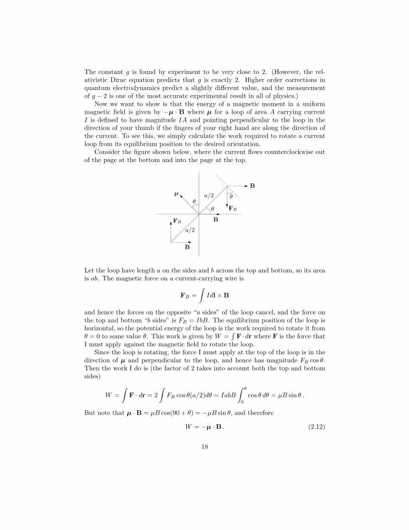
Consider the figure shown below, where the current flows counterclockwise outof the page at the bottom and into the page at the top.
B
B
B
FB
FB
a/2
a/2
θθ
θ
µ
Let the loop have length a on the sides and b across the top and bottom, so its areais ab. The magnetic force on a current-carrying wire is
FB =
∫Idl × B
and hence the forces on the opposite “a sides” of the loop cancel, and the force onthe top and bottom “b sides” is FB = IbB. The equilibrium position of the loop ishorizontal, so the potential energy of the loop is the work required to rotate it fromθ = 0 to some value θ. This work is given by W =
∫F ·dr where F is the force that
I must apply against the magnetic field to rotate the loop.Since the loop is rotating, the force I must apply at the top of the loop is in the
direction of µ and perpendicular to the loop, and hence has magnitude FB cos θ.Then the work I do is (the factor of 2 takes into account both the top and bottomsides)
W =
∫F · dr = 2
∫FB cos θ(a/2)dθ = IabB
∫ θ
0
cos θ dθ = µB sin θ .
But note that µ · B = µB cos(90 + θ) = −µB sin θ, and therefore
W = −µ · B . (2.12)
18
In this derivation, I never explicitly mentioned the torque on the loop due to B.However, we see that
‖N‖ = ‖r × FB‖ = 2(a/2)FB sin(90 + θ) = IabB sin(90 + θ)
= µB sin(90 + θ) = ‖µ× B‖
and thereforeN = µ× B . (2.13)
Note that W =∫‖N‖ dθ. We also see that
dL
dt=
d
dtr× p = r × dp
dt= r × F
where we used p = mv and r × p = v × p = 0. Therefore, as you should alreadyknow,
dL
dt= N . (2.14)
3 Mathematical Digression:
Rotations and Linear Transformations
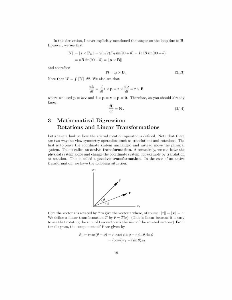
Let’s take a look at how the spatial rotation operator is defined. Note that thereare two ways to view symmetry operations such as translations and rotations. Thefirst is to leave the coordinate system unchanged and instead move the physicalsystem. This is called an active transformation. Alternatively, we can leave thephysical system alone and change the coordinate system, for example by translationor rotation. This is called a passive transformation. In the case of an activetransformation, we have the following situation:
x1
x2
r
r
θφ
Here the vector r is rotated by θ to give the vector r where, of course, ‖r‖ = ‖r‖ = r.We define a linear transformation T by r = T (r). (This is linear because it is easyto see that rotating the sum of two vectors is the sum of the rotated vectors.) Fromthe diagram, the components of r are given by
x1 = r cos(θ + φ) = r cos θ cosφ− r sin θ sinφ
= (cos θ)x1 − (sin θ)x2
19
x2 = r sin(θ + φ) = r sin θ cosφ+ r cos θ sinφ
= (sin θ)x1 + (cos θ)x2
or [x1
x2
]=
[cos θ − sin θ
sin θ cos θ
][x1
x2
]. (3.1)
Since T is a linear transformation, it is completely specified by defining its valueson a basis because
T (r) = T(∑
i
xiei
)=
∑
i
xiTei .
But Tei is just another vector in R2, and hence it can be expressed in terms of the
basis ei as
Tei =∑
j
ejaji . (3.2)
Be sure to note which indices are summed over in this expression. The matrix (aji)is called the matrix representation of the linear transformation T with respectto the basis ei. You will sometimes see this matrix written as [T ]e.
It is very important to realize that a linear transformation T takes the ith basisvector into the ith column of its matrix representation. This is easy to see if wewrite out the components of (3.2). Simply note that with respect to the basis ei,we have
e1 =
[1
0
]and e2 =
[0
1
]
and therefore
Tei = e1a1i + e2a2i =
[1
0
]a1i +
[0
1
]a2i =
[a1i
a2i
]
which is just the ith column of the matrix A = (aji).As an example, let V have a basis v1, v2, v3, and let T : V → V be the linear
transformation defined byTv1 = 3v1 + v3
Tv2 = v1 − 2v2 − v3
Tv3 = v2 + v3
Then the representation of T (relative to this basis) is
[T ]v =
3 1 00 −2 11 −1 1
.
Now let V be an n-dimensional vector space, and let W be a subspace of V .Let T be an operator on V , and suppose W has the property that Tw ∈ W for
20
every w ∈W . Then we say that W is T-invariant (or simply invariant when theoperator is understood).
What can we say about the matrix representation of T under these circum-stances? Well, let W have the basis w1, . . . , wr, and extend this to a basisw1, . . . , wr, v1, . . . , vn−r for V . Since Tw ∈ W for any w ∈W , we must have
Twi =
r∑
j=1
wjaji
for some set of scalars aji. But for any vi there is no such restriction since all weknow is that Tvi ∈ V . So we have
Tvi =r∑
j=1
wjbji +n−r∑
k=1
vkcki
for scalars bji and cki. Then since T takes the ith basis vector to the ith columnof the matrix representation [T ], we must have
[T ] =
[A B
0 C
]
where A is an r× r matrix, B is an r× (n− r) matrix, and C is an (n− r)× (n− r)matrix. Such a matrix is said to be a block matrix, and [T ] is in block triangularform.
Now let W be an invariant subspace of V . If it so happens that the subspaceof V spanned by the rest of the vectors v1, . . . , vn−r is also invariant, then thematrix representation of T will be block diagonal (because all of the bji in the aboveexpansion will be zero). As we shall see, this is in fact what happens when we addtwo angular momenta J1 and J2 and look at the representation of the rotationoperator with respect to the total angular momentum states (where J = J1 + J2).By choosing our states to be eigenstates of J2 and Jz rather than J1z and J2z, therotation operator becomes block diagonal rather than a big mess. This is becauserotations don’t change j, so for fixed j, the (2j + 1)-dimensional space spanned by|j − j〉, |j j − 1〉, . . . , |j j〉 is an invariant subspace under rotations. This changeof basis is exactly what Clebsch-Gordan coefficients accomplish.
Let us go back to our specific example of rotations. If we define r = T (r), thenon the the one hand we have
r =∑
j
xjej
while on the other hand, we can write
r = T (r) =∑
i
xiT (ei) =∑
i
∑
j
ejajixi .
21
Since the ej are a basis, they are linearly independent, and we can equate these lasttwo equations to conclude that
xj =∑
i
ajixi . (3.3)
Note which indices are summed over in this equation.Comparing (3.3) with (3.1), we see that the matrix in (3.1) is the matrix repre-
sentation of the linear transformation T defined by
(x1, x2) = T (x1, x2) = ((cos θ)x1 − (sin θ)x2, (sin θ)x1 + (cos θ)x2) .
Then the first column of [T ] is
T (e1) = T (1, 0) = (cos θ, sin θ)
and the second column is
T (e2) = T (0, 1) = (− sin θ, cos θ)
so that
[T ] =
[cos θ − sin θ
sin θ cos θ
]
as in (3.1).Using (3.3) we can make another extremely important observation. Since the
length of a vector is unchanged under rotations, we must have∑
j xj xj =∑
i xixi.But from (3.3) we see that
∑
j
xj xj =∑
i,k
ajiajkxixk
and hence it follows that∑
j
ajiajk =∑
j
aTijajk = δik . (3.4a)
In matrix notation, this isATA = I .
Since we are in a finite-dimensional space, this implies that AAT = I also. Inother words, AT = A−1. Such a matrix is said to be orthogonal. In terms ofcomponents, this second condition is
∑
j
aijaTjk =
∑
j
aijakj = δik . (3.4b)
It is also quite useful to realize that an orthogonal matrix is one whose rows (orcolumms) form an orthonormal set of vectors. If we let Ai denote the ith row of A,then from (3.4b) we have
Ai · Ak =∑
j
aijakj = δik .
22
Similarly, if we let Ai denote the ith column of A, then (3.4a) may be written
Ai · Ak =∑
j
ajiajk = δik .
Conversely, it is easy to see that any matrix whose rows (or columns) form anorthonormal set must be an orthogonal matrix.
In the case of complex matrices, repeating the above arguments using ‖x‖2 =∑i x
∗i xi, it is not hard to show that A†A = AA† = I where A† = A∗T . In this case,
the matrix A is said to be unitary. Thus a complex matrix is unitary if and only ifits rows (or columns) form an orthonormal set under the standard Hermitian innerproduct.
To describe a passive transformation, consider a linear transformation P actingon the basis vectors. In other words, we perform a change of basis defined by
ei = P (ei) =∑
j
ejpji .
In this situation, the linear transformation P is called the transition matrix.Suppose we have a linear operator A defined on our space. Then with respect to
a basis ei this operator has the matrix representation (aij) defined by (droppingthe parenthesis for simplicity)
Aei =∑
j
ejaji .
And with respect to another basis ei it has the representation (aij) defined by
Aei =∑
j
ej aji .
But ei = Pei, so the left side of this equation may be written
Aei = APei = A( ∑
j
ejpji
)=
∑
j
pjiAej =∑
j,k
pjiekakj =∑
j,k
ekakjpji
while the right side is∑
j
ej aji =∑
j
(Pej)aji =∑
j,k
ekpkj aji .
Equating these two expressions and using the linear independence of the ek we have∑
j
pkj aji =∑
j
akjpji
which in matrix notation is just PA = AP . Since each basis may be written interms of the other, the matrix P must be nonsingular so that P−1 exists, and hencewe have shown that
A = P−1AP . (3.5)
23
This extremely important equation relates the matrix representation of an op-erator A with respect to a basis ei to its representation A with respect to a basisei defined by ei = Pei. This is called a similarity transformation. In fact, thisis exactly what you do when you diagonalize a matrix. Starting with a matrix Arelative to a given basis, you first find its eigenvalues, and then use these to find thecorresponding eigenvectors. Letting P be the matrix whose columns are preciselythese eigenvectors, we then have P−1AP = D where D is a diagonal matrix withdiagonal entries that are just the eigenvalues of A.
4 Angular Momentum and Rotations
4.1 Angular Momentum as the Generator of Rotations
Before we begin with the physics, let me first prove an extremely useful mathemat-ical result. For any complex number (or matrix) x, let fn(x) = (1 + x/n)n, andconsider the limit
L = limn→∞
fn(x) = limn→∞
(1 +
x
n
)n.
Since the logarithm is a continuous function, we can interchange limits and the log,so we have
lnL = ln limn→∞
(1 +
x
n
)n= lim
n→∞ln
(1 +
x
n
)n
= limn→∞
n ln(1 +
x
n
)= lim
n→∞
ln(1 + x/n)
1/n.
As n → ∞, both the numerator and denominator go to zero, so we applyl’Hopital’s rule and take the derivative of both numerator and denominator withrespect to n:
lnL = limn→∞
(−x/n2)/(1 + x/n)
−1/n2= lim
n→∞
x
1 + x/n= x .
Exponentiating both sides, we have proved
limn→∞
(1 +
x
n
)n= ex . (4.1)
As I mentioned above, this result also applies if x is an n × n complex matrixA. This is a consequence of the fact (which I state without proof) that for any suchmatrix, the series
∞∑
n=0
An
n!
converges, and we take this as the definition of eA. (For a proof, see one of mylinear algebra books or almost any book on elementary real analysis or advancedcalculus.)
24
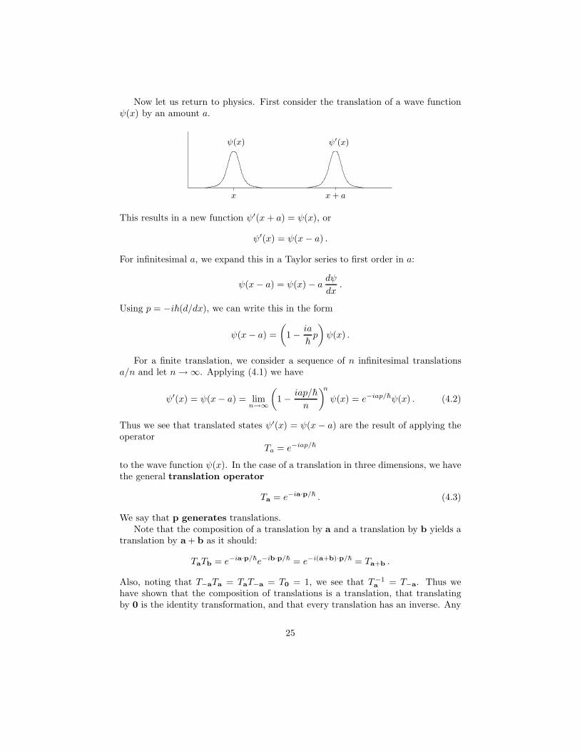
Now let us return to physics. First consider the translation of a wave functionψ(x) by an amount a.
x x+ a
ψ(x) ψ′(x)
This results in a new function ψ′(x+ a) = ψ(x), or
ψ′(x) = ψ(x− a) .
For infinitesimal a, we expand this in a Taylor series to first order in a:
ψ(x− a) = ψ(x) − adψ
dx.
Using p = −i~(d/dx), we can write this in the form
ψ(x− a) =
(1 − ia
~p
)ψ(x) .
For a finite translation, we consider a sequence of n infinitesimal translationsa/n and let n→ ∞. Applying (4.1) we have
ψ′(x) = ψ(x− a) = limn→∞
(1 − iap/~
n
)n
ψ(x) = e−iap/~ψ(x) . (4.2)
Thus we see that translated states ψ′(x) = ψ(x − a) are the result of applying theoperator
Ta = e−iap/~
to the wave function ψ(x). In the case of a translation in three dimensions, we havethe general translation operator
Ta = e−ia·p/~ . (4.3)
We say that p generates translations.Note that the composition of a translation by a and a translation by b yields a
translation by a + b as it should:
TaTb = e−ia·p/~e−ib·p/~ = e−i(a+b)·p/~ = Ta+b .
Also, noting that T−aTa = TaT−a = T0 = 1, we see that T−1a = T−a. Thus we
have shown that the composition of translations is a translation, that translatingby 0 is the identity transformation, and that every translation has an inverse. Any
25
collection of objects together with a composition law obeying closure, the existenceof an identity, and the existence of an inverse to every object in the collection issaid to form a group, and this group in particular is called the translation group.The composition of group elements is called group multiplication.
In the case of the translation group, is also important to realize that TaTb =TbTa. Any group with the property that multiplication is commutative is calledan abelian group. Another example of an abelian group is the set of all rotationsabout a fixed axis in R
3. (But the set of all rotations in three dimensions is mostdefinitely not abelian, as we are about to see.)
Now that we have shown that the linear momentum operator p generates transla-tions, let us show that the angular momentum operator is the generator of rotations.In particular, we will show explicitly that the orbital angular momentum operatorL generates spatial rotations in R
3. In the case of the spin operator S which actson the very abstract space of spin states, we will define rotations by analogy.
Let me make a slight change of notation and denote the rotated position vectorby a prime instead of a bar. If we rotate a vector x in R
3, then we obtain a newvector x′ = R(θ)x where R(θ) is the matrix that represents the rotation. In twodimensions this is [
x′
y′
]=
[cos θ − sin θ
sin θ cos θ
][x
y
].
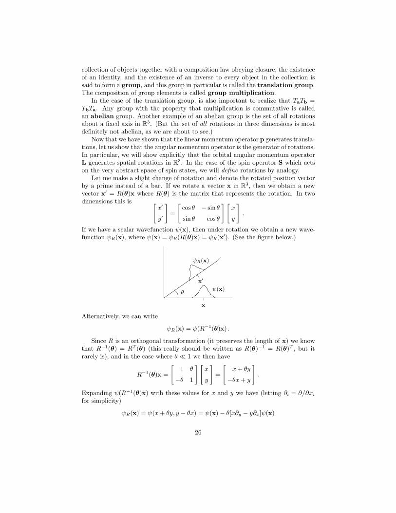
If we have a scalar wavefunction ψ(x), then under rotation we obtain a new wave-function ψR(x), where ψ(x) = ψR(R(θ)x) = ψR(x′). (See the figure below.)
x
x′
θψ(x)
ψR(x)
Alternatively, we can write
ψR(x) = ψ(R−1(θ)x) .
Since R is an orthogonal transformation (it preserves the length of x) we knowthat R−1(θ) = RT (θ) (this really should be written as R(θ)−1 = R(θ)T , but itrarely is), and in the case where θ ≪ 1 we then have
R−1(θ)x =
[1 θ
−θ 1
][x
y
]=
[x+ θy
−θx+ y
].
Expanding ψ(R−1(θ)x) with these values for x and y we have (letting ∂i = ∂/∂xi
for simplicity)
ψR(x) = ψ(x+ θy, y − θx) = ψ(x) − θ[x∂y − y∂x]ψ(x)
26
or, using pi = −i~∂i this is
ψR(x) = ψ(x) − i
~θ[xpy − ypx]ψ(x) =
(1 − i
~θLz
)ψ(x) .
Thus we see that angular momentum is indeed the generator of rotations.For finite θ we exponentiate this to write ψR(x) = e−(i/~)θLzψ(x), and in the
case of an arbitrary angle θ in R3 this becomes
ψR(x) = e−(i/~)θ·Lψ(x) . (4.4)
In an abstract notation we write this as
|ψR〉 = U(R)|ψ〉
where U(R) = e−(i/~)θ·L. For simplicity and clarity, we have written U(R) ratherthan the more complete U(R(θ)), which we continue to do unless the more completenotation is needed.
What we just did was for orbital angular momentum. In the case of spin thereis no classical counterpart, so we define the spin angular momentum operator S toobey the usual commutation relations, and then the spin states will transform underthe rotation operator e−(i/~)θ·S. (We will come back to justifying this at the endof this section.) It is common to use the symbol J to stand for any type of angularmomentum operator, for example L,S or L + S, and this is what we shall do fromnow on. In the case where J = L + S, J is called the total angular momentum
operator.(The example above applied to a scalar wavefunction ψ, which represents a
spinless particle. Particles with spin are described by vector wavefunctionsψ, and inthis case the spin operator S serves to mix up the components of ψ under rotations.)
The angular momentum operators J2 = J · J and Jz commute, and hence theyhave simultaneous eigenstates, denoted by |jm〉, with the property that (with ~ = 1)
J2|jm〉 = j(j + 1)|jm〉 and Jz|jm〉 = m|jm〉
where m takes the 2j + 1 values −j ≤ m ≤ j. Since the rotation operator is givenby U(R) = e−iθ·J we see that [U(R), J2] = 0. Then
J2U(R)|jm〉 = U(R)J2|jm〉 = j(j + 1)U(R)|jm〉
so that the magnitude of the angular momentum can’t change under rotations.However, [U(R), Jz] 6= 0 so the rotated state will no longer be an eigenstate of Jz
with the same eigenvalue m.Note that acting to the right we have the matrix element
〈j′m′|J2U(R)|jm〉 = 〈j′m′|U(R)J2|jm〉 = j(j + 1)〈j′m′|U(R)|jm〉
while acting to the left gives
〈j′m′|J2U(R)|jm〉 = j′(j′ + 1)〈j′m′|U(R)|jm〉
27
and therefore〈j′m′|U(R)|jm〉 = 0 unless j = j′ . (4.5)
We also make note of the fact that acting with J2 and Jz in both directions yields
〈j′m′|J2|jm〉 = j′(j′ + 1)〈j′m′|jm〉 = j(j + 1)〈j′m′|jm〉
and〈jm′|Jz|jm〉 = m′〈jm′|jm〉 = m〈jm′|jm〉
so that (as you should have already known)
〈j′m′|jm〉 = δj′jδm′m . (4.6)
In other words, the states |jm〉 form a complete orthonormal set, and the stateU(R)|jm〉 must be of the form
U(R)|jm〉 =∑
m′
|jm′〉〈jm′|U(R)|jm〉 =∑
m′
|jm′〉D(j)m′m(θ) (4.7)
whereD
(j)m′m(θ) := 〈jm′|U(R)|jm〉 = 〈jm′|e−iθ·J|jm〉 . (4.8)
(Notice the order of susbscripts in the sum in equation (4.7). This is the same asthe usual definition of the matrix representation [T ]e = (aij) of a linear operatorT : V → V defined by Tei =
∑j ejaji.)
Since for each j there are 2j + 1 values of m, we have constructed a (2j +1) × (2j + 1) matrix D(j)(θ) for each value of j. This matrix is referred to as thejth irreducible representation of the rotation group. The word “irreducible”means that there is no subset of the space of states |jj〉, |j,m − 1〉, . . . , |j,−j〉that transforms into itself under all rotations U(R(θ)). Put in another way, arepresentation is irreducible if the vector space on which it acts has no invariantsubspaces.
Now, it is a general result of the theory of group representations that any repre-sentation of a finite group or compact Lie group is equivalent to a unitary represen-tation, and any reducible unitary representation is completely reducible. Therefore,any representation of a finite group or compact Lie group is either already irre-ducible or else it is completely reducible (i.e., the space on which the operators actcan be put into block diagonal form where each block corresponds to an invariantsubspace). However, at this point we don’t want to get into the general theoryof representations, so let us prove directly that the representations D(j)(θ) of therotation group are irreducible.
Recall that the raising and lowering operators J± are defined by
J±|jm〉 = (Jx ± iJy)|jm〉 =√j(j + 1) −m(m± 1) |j,m± 1〉 .
In particular, the operators J± don’t change the value of j when acting on the states|jm〉. (This is just the content of equation (1.4).)
28
Theorem 4.1. The representations D(j)(θ) of the rotation group are irreducible.
In other words, there is no subset of the space of states |jm〉 (for fixed j) thattransforms among itself under all rotations.
Proof. Fix j and let V be the space spanned by the 2j + 1 vectors |jm〉 := |m〉.We claim that V is irreducible with respect to rotations U(R). This means thatgiven any |u〉 ∈ V , the set of all vectors of the form U(R)|u〉 (i.e., for all rotationsU(R)) spans V . (Otherwise, if there exists |v〉 such that U(R)|v〉 didn’t span V ,then V would be reducible since the collection of all such U(R)|v〉 would define aninvariant subspace.)
To show V is irreducible, let V = SpanU(R)|u〉 where |u〉 ∈ V is arbitrary butfixed. For infinitesimal θ we have U(R(θ)) = e−iθ·J = 1 − iθ · J and in particularU(R(εx)) = 1 − iεJx and U(R(εy)) = 1 − iεJy. Then
J±|u〉 = (Jx ± iJy)|u〉 =
1
iε[1 − U(R(εx))] ± i
(1
iε[1 − U(R(εy))]
)|u〉
=1
ε
± [1 − U(R(εy))] − i+ iU(R(εx))
|u〉 ∈ V
by definition of V and vector spaces. Since J± acting on |u〉 is a linear combination
of rotations acting on |u〉 and this is in V , we see that (J±)2 acting on |u〉 is again
some other linear combination of rotations acting on |u〉 and hence is also in V . So
in general, we see that (J±)n|u〉 is again in V .By definition of V , we may write (since j is fixed)
|u〉 =∑
m
|jm〉〈jm|u〉 =∑
m
|m〉〈m|u〉
= |m〉〈m|u〉 + |m+ 1〉〈m+ 1|u〉 + · · · + |j〉〈j|u〉
where m is simply the smallest value of m for which 〈m|u〉 6= 0 (and not all ofthe terms up to 〈j|u〉 are necessarily nonzero). Acting on this with J+ we obtain(leaving off the constant factors and noting that J+|j〉 = 0)
J+|u〉 ∼ |m+ 1〉〈m|u〉 + |m+ 2〉〈m+ 1|u〉 + · · · + |j〉〈j − 1|u〉 ∈ V .
Since 〈m|u〉 6= 0 by assumption, it follows that |m+ 1〉 ∈ V .We can continue to act on |u〉 with J+ a total of j −m times at which point we
will have shown that |m+ j −m〉 = |j〉 := |jj〉 ∈ V . Now we can apply J− 2j + 1
times to |jj〉 to conclude that the 2j + 1 vectors |jm〉 all belong to V , and thus
V = V . (This is because we have really just applied the combination of rotations
(J−)2j+1(J+)j−m to |u〉, and each step along the way is just some vector in V .)
As the last subject of this section, let us go back and show that e−(i/~)θ·S reallyrepresents a rotation in spin space. Let R denote the unitary rotation operator, and
29
let A be an arbitrary observable. Rotating our system, a state |ψ〉 is transformedinto a rotated state |ψR〉 = R|ψ〉. In the original system, a measurement of Ayields the result 〈ψ|A|ψ〉. Under rotations, we measure a rotated observable AR inthe rotated states. Since the physical results of a measurement can’t change justbecause of our coordinate description, we must have
〈ψR|AR|ψR〉 = 〈ψ|A|ψ〉 .
But〈ψR|AR|ψR〉 = 〈ψ|R†ARR|ψ〉
and hence we have R†ARR = A or
AR = RAR† = RAR−1 . (4.9)
(Compare this to (3.5). Why do you think there is a difference?)Now, what about spin one-half particles? To say that a measurement of the spin
in a particular direction m can only yield one of two possible results means that theoperator S · m has only the two eigenvalues ±~/2. Let us denote the correspondingstates by |m±〉. In other words, we have
(S · m)|m±〉 = ±~
2|m±〉 .
(This is just the generalization of (2.1c) for the case of spin one-half. It also appliesto arbitrary spin if we write (S · m)|mms〉 = ms|mms〉.)
Let us rotate the unit vector m by θ to obtain another unit vector n, andconsider the operator
e−(i/~)θ·S(S · m)e(i/~)θ·S .
Acting on the state e−(i/~)θ·S|m±〉 we have
[e−(i/~)θ·S(S · m)e(i/~)θ·S]e−(i/~)θ·S|m±〉 = e−(i/~)θ·S(S · m)|m±〉
= ±~
2e−(i/~)θ·S|m±〉 .
Therefore, if we define the rotated state
|n±〉 := e−(i/~)θ·S|m±〉 (4.10a)
we see from (4.9) that we also have the rotated operator
S · n := e−(i/~)θ·S(S · m)e(i/~)θ·S (4.10b)
with the property that
(S · n)|n±〉 = ±~
2|n±〉 (4.10c)
as it should. This shows that e−(i/~)θ·S does indeed act as the rotation operator onthe abstract spin states.
30
What we have shown then, is that starting from an eigenstate |m±〉 of the spinoperator S · m, we rotate by an angle θ to obtain the rotated state |n±〉 that is aneigenstate of S · n with the same eigenvalues.
For spin one-half we have S = σ/2 (with ~ = 1), and using (2.8), you can showthat the rotation operator becomes
e−iσ·θ/2 =∞∑
m=0
(−iσ · θ/2)n
n!
= I cosθ
2− iσ · θ sin
θ
2. (4.11)
Example 4.1. Let us derive equations (2.9) using our rotation formalism. We startby letting m = z and n = x, so that θ = (π/2)y. Then the rotation operator is
R(θ) = e−iπσy/4 = I cosπ
4− iσy sin
π
4
=
[cosπ/4 − sinπ/4
sinπ/4 cosπ/4
]=
1√2
[1 −1
1 1
].
Acting on the state|m+〉 = |z+〉
we have
R(θ)|z+〉 =1√2
[1 −1
1 1
][1
0
]=
1√2
[1
1
]= |x+〉
which is just (2.9a). Similarly, it is also easy to see that
R(θ)|z−〉 =1√2
[1 −1
1 1
][0
1
]=
−1√2
[1
−1
]= |x−〉
which is the same as (2.9b) up to an arbitrary phase.So far we have shown that the rotation operator R(θ) = R((π/2)y) indeed takes
the eigenstates of Sz into the eigenstates of Sx. Let us also show that it takesSz = σz/2 into Sx = σx/2. This is a straightforward computation:
e−iπσy/4σzeiπσy/4 =
1√2
[1 −1
1 1
] [1 0
0 −1
]1√2
[1 1
−1 1
]
=1
2
[0 2
2 0
]=
[0 1
1 0
]= σx
as it should.
31
4.2 Spin Dynamics in a Magnetic Field
As we mentioned at the beginning of Section 2, a particle of charge q and mass mmoving in a circular orbit has a magnetic moment given classically by
µl =q
2mcL .
This relation is also true in quantum mechanics for orbital angular momentum, butfor spin angular momentum we must write
µs = gq
2mcS (4.12)
where the constant g is called a g-factor. For an electron, g is found by experimentto be very close to 2. (The Dirac equation predicts that g = 2 exactly, and higherorder correction in QED show a slight deviation from this value.) And for a proton,g = 5.59. Furthermore, electrically neutral particles such as the neutron also havemagnetic moments, which you can think of as arising from some sort of internalcharge distribution or current. (But don’t think too hard.)
In the presence of a magnetic field B(t), a magnetic moment µ feels an appliedtorque µ×B, and hence possesses a potential energy −µ·B. Because of this torque,the magnetic moment (and hence the particle) will precess about the field. (Recallthat torque is equal to the time rate of change of angular momentum, and hence anon-zero torque means that the angular momentum vector of the particle must bechanging.) Let us see what we can learn about this precession.
We restrict consideration to particles essentially at rest (i.e., with no angularmomentum) in a uniform magnetic field B(t), and write µs = γS where γ = gq/2mcis called the gyromagnetic ratio. (If the field isn’t uniform, there will be a forceequal to the negative gradient of the potential energy, and the particle will move inspace. This is how the Stern-Gerlach experiment works, as we will see below.) Inthe case of a spin one-half particle, the Hamiltonian given by
Hs = −µs · B(t) = − gq
2mcS · B(t) = − gq~
4mcσ · B(t) . (4.13)
To understand how spin behaves, we look at this motion from the point of view ofthe Heisenberg picture, which we now describe. (See Griffiths, Example 4.3 for asomewhat different approach.)
The formulation of quantum mechanics that we have used so far is called theSchrodinger picture (SP). In this formulation, the operators are independent oftime, but the states (wave functions) evolve in time. The stationary state solutionsto the Schrodinger equation
H |Ψ(t)〉 = i~∂
∂t|Ψ(t)〉
(where H is independent of time) are given by
|Ψ(t)〉 = e−iEt/~|ψ〉 = e−iHt/~|ψ〉 (4.14)
32
where H |ψ〉 = E|ψ〉 and |ψ〉 is independent of time.In the Heisenberg picture (HP), the states are independent of time, and the
operators evolve in time according to an equation of motion. To derive the equationsof motion for the operators in this picture, we freeze out the states at time t = 0:
|ψH〉 := |Ψ(0)〉 = |ψ〉 = e+iHt/~|Ψ(t)〉 . (4.15a)
In the SP, the expectation value of an observable O (possibly time dependent) isgiven by
〈O〉 = 〈Ψ(t)|O|Ψ(t)〉 = 〈ψ|eiHt/~Oe−iHt/~|ψ〉 .In the HP, we want the same measurable result for 〈O〉, so we have
〈O〉 = 〈ψH |OH |ψH〉 = 〈ψ|OH |ψ〉 .
Equating both versions of these expectation values, we conclude that
OH = eiHt/~Oe−iHt/~ (4.15b)
where OH = OH(t) is the representation of the observable O in the HP. Note inparticular that the Hamiltonian is the same in both pictures because
HH = eiHt/~He−iHt/~ = eiHt/~e−iHt/~H = H .
Now take the time derivative of (4.15b) and use the fact that H commutes withe±iHt/~:
dOH
dt=i
~HeiHt/~Oe−iHt/~ − i
~eiHt/~Oe−iHt/~H + eiHt/~
∂O∂te−iHt/~
=i
~[H,OH ] + eiHt/~
∂O∂te−iHt/~ .
If O has no explicit time dependence (for example, the operator pt has explicit timedependence), then this simplifies to the Heisenberg equation of motion
dOH
dt=i
~[H,OH ] . (4.16)
Also note that if H is independent of time, then so is HH = H , and (4.16) thenshows that H = const and energy is conserved.
Returning to our problem, we use the Hamiltonian (4.13) in the equation ofmotion (4.16) to write
dSi
dt=i
~[Hs, Si] = − i
~
gq
2mcBj [Sj , Si] = − i
~
gq
2mcBji~εjikSk
= +gq
2mcεikjSkBj =
gq
2mc(S× B)i
ordS(t)
dt=
gq
2mcS(t) × B(t) = µs(t) × B(t) . (4.17)
33
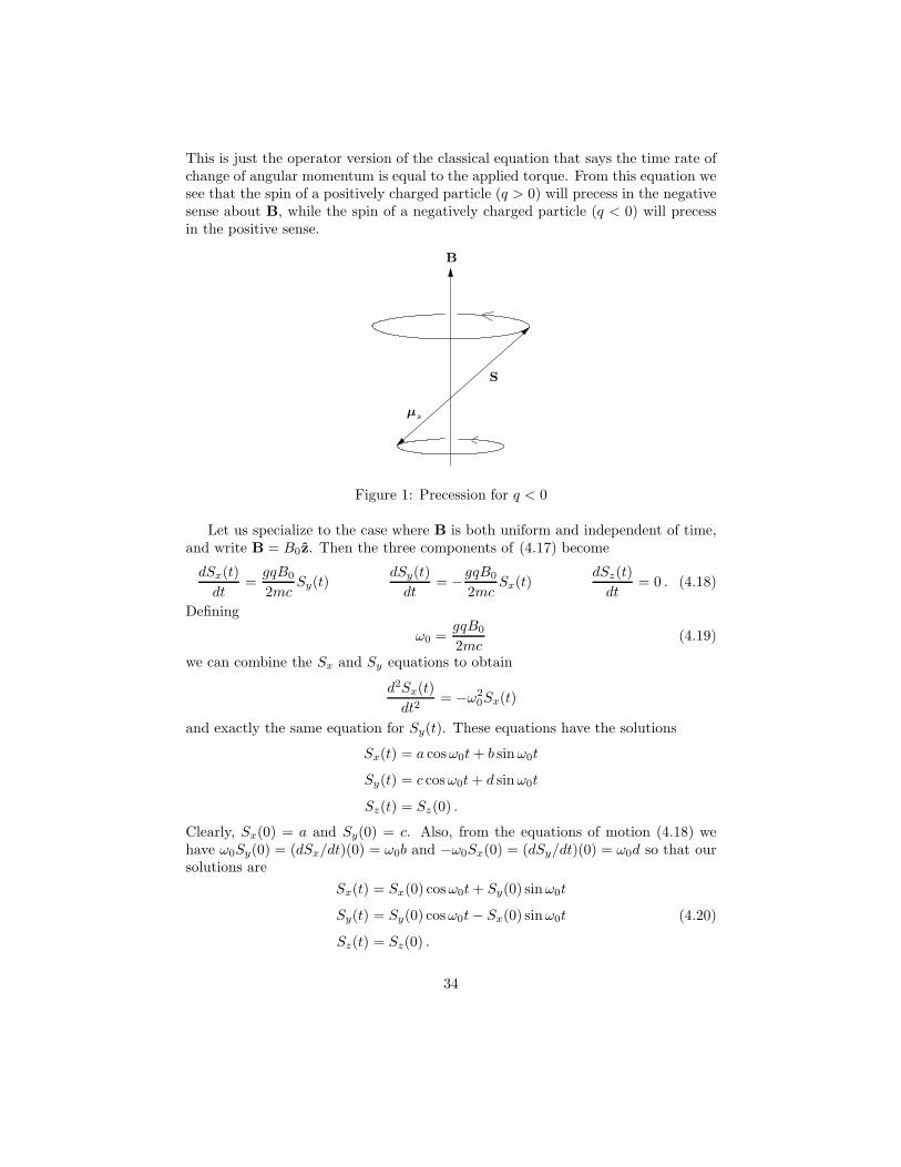
This is just the operator version of the classical equation that says the time rate ofchange of angular momentum is equal to the applied torque. From this equation wesee that the spin of a positively charged particle (q > 0) will precess in the negativesense about B, while the spin of a negatively charged particle (q < 0) will precessin the positive sense.
S
µs
B
Figure 1: Precession for q < 0
Let us specialize to the case where B is both uniform and independent of time,and write B = B0z. Then the three components of (4.17) become
dSx(t)
dt=gqB0
2mcSy(t)
dSy(t)
dt= −gqB0
2mcSx(t)
dSz(t)
dt= 0 . (4.18)
Defining
ω0 =gqB0
2mc(4.19)
we can combine the Sx and Sy equations to obtain
d2Sx(t)
dt2= −ω2
0Sx(t)
and exactly the same equation for Sy(t). These equations have the solutions
Sx(t) = a cosω0t+ b sinω0t
Sy(t) = c cosω0t+ d sinω0t
Sz(t) = Sz(0) .
Clearly, Sx(0) = a and Sy(0) = c. Also, from the equations of motion (4.18) wehave ω0Sy(0) = (dSx/dt)(0) = ω0b and −ω0Sx(0) = (dSy/dt)(0) = ω0d so that oursolutions are
Sx(t) = Sx(0) cosω0t+ Sy(0) sinω0t
Sy(t) = Sy(0) cosω0t− Sx(0) sinω0t
Sz(t) = Sz(0) .
(4.20)
34
These can be written in the form Sx(t) = A cos(ω0t+δx) and Sy(t) = A sin(ω0t+δy)where A2 = Sx(0)2+Sy(0)2. Since these are the parametric equations of a circle, wesee that S precesses about the B field, with a constant projection along the z-axis.
For example, suppose the spin starts out at t = 0 in the xy-plane as an eigenstateof Sx with eigenvalue +~/2. This means that
〈Sx(0)〉 = 〈x + |Sx(0)|x+〉 =~
2
〈Sy(0)〉 = 〈Sz(0)〉 = 0 .
Taking the expectation value of equations (4.20) we see that
〈Sx(t)〉 =~
2cosω0t 〈Sy(t)〉 = −~
2sinω0t 〈Sz(t)〉 = 0 . (4.21)
This clearly shows that the spin stays in the xy-plane, and precesses about the z-axis. The direction of precession depends on the sign of ω0, which in turn dependson the sign of q as defined by (4.19).
How does this look from the point of view of the SP? From (4.14), the spin stateevolves according to
|χ(t)〉 = e−iHt/~|χ(0)〉 = ei(gqBt/2mc)Sz/~|χ(0)〉 = eiω0tSz/~|χ(0)〉 .
Comparing this with (4.10a), we see that in the SP the spin precesses about −z
with angular velocity ω0.Now let us consider the motion of an electron in an inhomogeneous magnetic
field. Since for the electron we have q = −e < 0, we see from (4.12) that µs is anti-parallel to the spin S. The potential energy is Hs = −µs ·B, and as a consequence,the force on the electron is
F = −∇Hs = ∇(µs · B) .
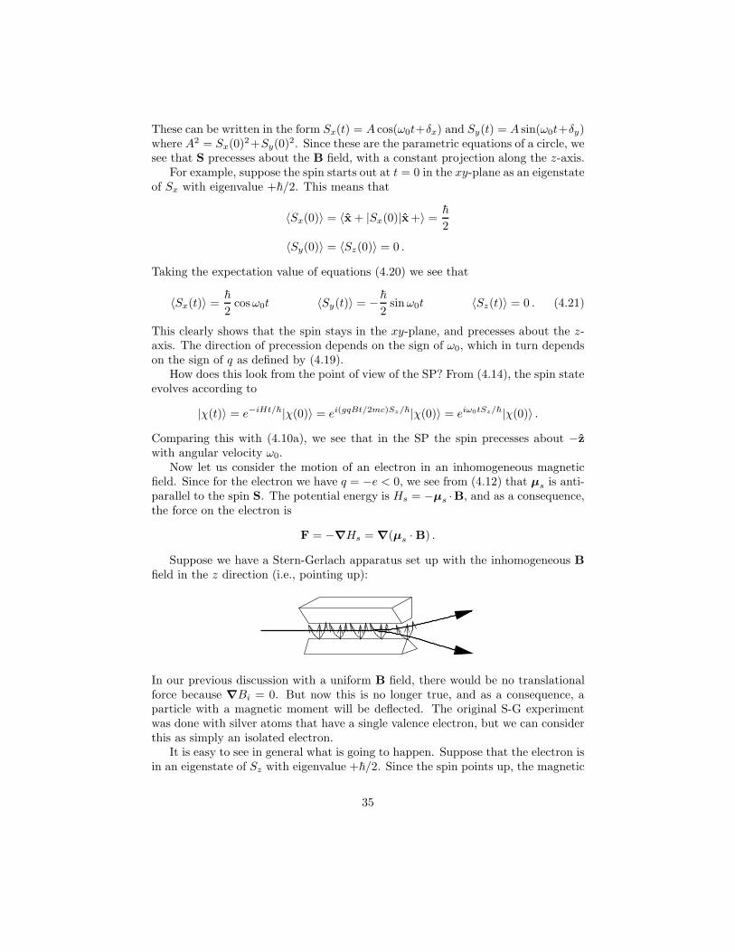
Suppose we have a Stern-Gerlach apparatus set up with the inhomogeneous B
field in the z direction (i.e., pointing up):
In our previous discussion with a uniform B field, there would be no translationalforce because ∇Bi = 0. But now this is no longer true, and as a consequence, aparticle with a magnetic moment will be deflected. The original S-G experimentwas done with silver atoms that have a single valence electron, but we can considerthis as simply an isolated electron.
It is easy to see in general what is going to happen. Suppose that the electron isin an eigenstate of Sz with eigenvalue +~/2. Since the spin points up, the magnetic
35
moment µs is anti-parallel to B, and hence Hs = −µs · B > 0. Since the electronwants to minimize its energy, it will travel towards a region of smaller B, which isup. Obviously, if the spin points down, then µs is parallel to B and Hs < 0 so theelectron will decrease its energy by moving to a region of larger B, which is down.
Another way to look at this is from the force relation. If µs is anti-parallel toB (i.e., spin up), then since the gradient of B is negative (the B field is decreasingin the positive direction), the force on the electron will be in the positive direction,and hence the electron will be deflected upwards. Similarly, if the spin is down,then the force will be negative and the electron is deflected downwards.
It is worth pointing out that a particle with angular momentum l will split into2l + 1 distinct components. So if the magnetic moment is due to orbital angularmomentum, then there will necessarily be an odd number of beams coming out ofa S-G apparatus. Therefore, the fact that an electron beam splits into two beamsshows that its angular momentum can not be due to orbital motion, and hence is agood experimental verification of the existence of spin.
Suppose that the particle enters the S-G apparatus at t = 0 with its spin alignedalong x, and emerges at time t = T . If the magnetic field were uniform, then theexpectation value of S at t = T would be given by equations (4.21) as
〈S〉unifT =
~
2(cosω0T )x− ~
2(sinω0T )y . (4.22)
Interestingly, for the inhomogeneous field this expectation value turns out to bezero.
To see this, let the particle enter the apparatus with its spin along the x direction,and let its initial spatial wave function be the normalized wave packet ψ0(r, t). Interms of the eigenstates of Sz, the total wave function at t = 0 is then (from (2.9a))
Ψ(r, 0) =1√2
[ψ0(r, 0)
ψ0(r, 0)
]. (4.23a)
When the particle emerges at t = T , it is a superposition of localized spin up wavepackets ψ+(r, T ) and spin down wave packets ψ−(r, T ):
Ψ(r, T ) =1√2
[ψ+(r, T )
ψ−(r, T )
]. (4.23b)
Since the spin up and spin down states are well separated, there is no overlapbetween these wave packets, and hence we have
ψ+(r, T )ψ−(r, T ) ≈ 0 . (4.23c)
Since the B field is essentially in the z direction there is no torque on theparticle in the z direction, and from (4.17) it follows that the z component of spinis conserved. In other words, the total probability of finding the particle with spin
36
up at t = T is the same as it is at t = 0. The same applies to the spin down states,so we have ∫
|ψ+(r, T )|2 d3r =
∫|ψ0(r, 0)|2 d3r
and ∫|ψ−(r, T )|2 d3r =
∫|ψ0(r, 0)|2 d3r
and therefore ∫|ψ+(r, T )|2 d3r =
∫|ψ−(r, T )|2 d3r . (4.24)
From (4.23a), the expectation value of S at r and t = 0 is given by
〈S〉r,0 = Ψ†(r, 0)~
2σΨ(r, 0)
= Ψ†(r, 0)~
2(σxx + σyy + σzz)Ψ(r, 0)
=~
2|ψ0(r, 0)|2 x
and hence the net expectation value at t = 0 is (since ψ0 is normalized)
〈S〉0 =
∫〈S〉r,0 d
3r =~
2x .
(This should have been expected since the particle entered the apparatus with itsspin in the x direction.) And from (4.23b), using (4.23c) we have for the exitingparticle
〈S〉r,T = Ψ†(r, T )~
2σΨ(r, T )
= Ψ†(r, T )~
2(σxx + σyy + σz z)Ψ(r, T )
=~
2
|ψ+(r, T )|2 − |ψ−(r, T )|2
z .
Integrating over all space, we see from (4.24) that
〈S〉inhomT = 0 (4.25)
as claimed.Why does the uniform field give a non-zero value for 〈S〉T whereas the inhomo-
geneous field gives zero? The answer lies with (4.19). Observe that the precessionalfrequency ω0 depends on the field B. In the Stern-Gerlach apparatus, the B field isweaker up high and stronger down low. This means that particles lower in the beamprecess at a faster rate than particles higher in the beam. Since (4.25) is essentially
37
an average of (4.22), we see that the different phases due to the different values ofω0 will cause the integral to vanish.
Of course, this assumes that there is sufficient variation ∆ω0 in precessionalfrequencies that the trigonometric functions average to zero. This will be true aslong as
(∆ω0)T ≥ 2π .
In fact, this places a constraint on the minimum amount of inhomogeneity that theS-G apparatus must have in order to split the beam. From (4.19) we have
∆ω0 = − e
mec∆B0 ≈ − e
mec
∂B0
∂z∆z
where ∆z is the distance between the poles of the magnet. Therefore, in order forthe apparatus to work we must have
∣∣∣∣e
mec
∂B0
∂z
∣∣∣∣T ≥ 2π
∆z.
5 The Addition of Angular Momentum
The basic idea is simply to express the eigenstates of the total angular momentumoperator J of two particles in terms of the eigenstates of the individual angularmomentum operators J1 and J2, where J = J1 + J2. (Alternatively, this could bethe addition of spin and orbital angular momenta of a single particle, etc.) Eachparticle’s angular momentum operator satisfies (where the subscript a labels theparticle and where we take ~ = 1)
[Jai, Jaj ] = i
3∑
k=1
εijkJak
with corresponding eigenstate |jama〉. And since we assume that [J1,J2] = 0, itfollows that
[Ji, Jj ] = [J1i + J2i, J1j + J2j ] = [J1i, J1j ] + [J2i, J2j ]
= i
3∑
k=1
εijkJ1k + i
3∑
k=1
εijkJ2k = i
3∑
k=1
εijk
(J1k + J2k
)
= i
3∑
k=1
εijkJk
and hence J is just another angular momentum operator with eigenstates |jm〉.Next we want to describe simultaneous eigenstates of the total angular momen-
tum. From [J1,J2] = 0, it is clear that [J12, J2
2] = 0, and since [Ja2, Jaz] = 0, we
see that we can choose our states to be simultaneous eigenstates of J12, J2
2, J1z
and J2z . We denote these states by |j1j2m1m2〉.
38
Alternatively, we can choose our states to be simultaneous eigenstates of J2,J1
2, J22 and Jz . That [J2, Jz ] = 0 follows directly because J is just an angular
momentum operator. And the fact that [Ja2, Jz] = 0 follows because Ja is an
angular momentum operator, Jz = J1z +J2z and [J1,J2] = 0. Finally, to show that[J2, Ja
2] = 0, we simply observe that
J2 =(J1 + J2
)2
= J12 + J2
2 + 2J1 · J2
= J12 + J2
2 + 2(J1xJ2x + J1yJ2y + J1zJ2z) .
It is now easy to see that [J2, Ja2] = 0 because [J1,J2] = 0 and [Ja
2, Jai] = 0 fori = x, y, z. We denote these simultaneous eigenstates by |j1j2jm〉.
However, let me emphasize that even though [J2, Jz] = 0, it is not true that[J2, Jaz ] = 0. This means that we can not specify J2 in the states |j1j2m1m2〉, andwe can not specify either J1z or J2z in the states |j1j2jm〉.
We know that the angular momentum operators and states satisfy (with ~ = 1)
J2|jm〉 = j(j + 1)|jm〉 (5.1a)
Jz|jm〉 = m|jm〉 (5.1b)
J±|jm〉 =√j(j + 1) −m(m± 1)|jm± 1〉 . (5.1c)
Let us denote the two individual angular momentum states by |j1m1〉 and |j2m2〉.Then the two-particle basis states are denoted by the various forms (see Part I,Section 1 in the handout Supplementary Notes on Mathematics)
|j1j2m1m2〉 = |j1m1〉|j2m2〉 = |j1m1〉 ⊗ |j2m2〉 .
When we write 〈j1j2m1m2|j′1j′2m′1m
′2〉 we really mean
(〈j1m1| ⊗ 〈j2m2|)(|j′1m′1〉 ⊗ |j′2m′
2〉) = 〈j1m1|j′1m′1〉〈j2m2|j′2m′
2〉 .
Since these two-particle states form a complete set, we can write the total com-bined angular momentum state of both particles as
|j1j2jm〉 =∑
j′1j′2
m1m2
|j′1j′2m1m2〉〈j′1j′2m1m2|j1j2jm〉 . (5.2)
However, we now show that many of the matrix elements 〈j′1j′2m1m2|j1j2jm〉 vanish,and hence the sum will be greatly simplified.
For our two-particle operators we have
Jz = J1z + J2z and J± = J1± + J2± .
39
While we won’t really make any use of it, let me point out the correct way to writeoperators when dealing with tensor (or direct) product states. In this case we shouldproperly write operators in the form
J = J1 ⊗ 12 + 11 ⊗ J2 .
Then acting on the two-particle states we have, for example,
Jz(|j1m1〉 ⊗ |j2m2〉) =[J1z ⊗ 1 + 1 ⊗ J2z
](|j1m1〉 ⊗ |j2m2〉)
= J1z|j1m1〉 ⊗ |j2m2〉 + |j1m1〉 ⊗ J2z|j2m2〉
= (m1 +m2)(|j1m1〉 ⊗ |j2m2〉) .
As I said, while we won’t generally write out operators and states in this form, youshould keep in mind what is really going on.
Now, for our two-particle states we have
Ja2|j1j2m1m2〉 = ja(ja + 1)|j1j2m1m2〉
Jaz |j1j2m1m2〉 = ma|j1j2m1m2〉
where a = 1, 2. Taking the matrix element of J12 acting to both the left and right
we see that
〈j′1j′2m1m2|J12|j1j2jm〉 = j′1(j
′1 + 1)〈j′1j′2m1m2|j1j2jm〉
= 〈j′1j′2m1m2|j1j2jm〉j1(j1 + 1)
or[j′1(j
′1 + 1) − j1(j1 + 1)]〈j′1j′2m1m2|j1j2jm〉 = 0 .
Since this result clearly applies to J22 as well, we must have
〈j′1j′2m1m2|j1j2jm〉 = 0 if j′1 6= j1 or j′2 6= j2 .
In other words, equation (5.2) has simplified to
|j1j2jm〉 =∑
m1m2
|j1j2m1m2〉〈j1j2m1m2|j1j2jm〉 .
Next, from Jz = J1z + J2z we can let J1z + J2z act to the left and Jz act to theright so that
〈j1j2m1m2|Jz|j1j2jm〉 = (m1 +m2)〈j1j2m1m2|j1j2jm〉= 〈j1j2m1m2|j1j2jm〉m.
This shows that
〈j1j2m1m2|j1j2jm〉 = 0 unless m = m1 +m2
40
and hence equation (5.2) has become
|j1j2jm〉 =∑
m1m2
m1+m2=m
|j1j2m1m2〉〈j1j2m1m2|j1j2jm〉 .
Finally, we regard the values of j1 and j2 as fixed and understood, and we simplywrite the total angular momentum state as
|jm〉 =∑
m1m2
m1+m2=m
|m1m2〉〈m1m2|jm〉 . (5.3)
The complex numbers 〈m1m2|jm〉 are called Clebsch-Gordan coefficients.They are really nothing more than the elements of the unitary transition matrix thattakes us from the |m1m2〉 basis to the |jm〉 basis. (This is just the statementfrom linear algebra that given two bases ei and ei of a vector space V , there isa nonsingular transition matrix P such that ei =
∑j ejpji. Moreover, ei is just the
ith column of P . If both bases are orthonormal, then P is in fact a unitary matrix.See Theorem 15 in Supplementary Notes on Mathematics.)
Since (normalized) eigenfunctions corresponding to distinct eigenvalues of a her-mitian operator are orthonormal, we know that
〈j′m′|jm〉 = δjj′δmm′ and 〈m′1m
′2|m1m2〉 = δm1m′
1δm2m′
2.
Therefore, taking the inner product of equation (5.3) with itself we see that
∑
m1m2
m1+m2=m
|〈m1m2|jm〉|2 = 1 . (5.4)
Given j1 and j2, this holds for any resulting values of j and m. (This is reallyjust another way of saying that the columns of the unitary transition matrix arenormalized.)
Now, we know that −j1 ≤ m1 ≤ j1 and −j2 ≤ m2 ≤ j2. Therefore, fromm = m1 +m2, the maximum value of m must be j1 + j2. And since −j ≤ m ≤ j,it follows that the maximum value of j is jmax = j1 + j2. Corresponding to thismaximum value j1 + j2 of j, we have a multiplet of 2(j1 + j2) + 1 values of m, i.e.,−(j1 + j2) ≤ m ≤ j1 + j2. On the other hand, since there are 2j1 + 1 possiblevalues of m1, and 2j2 +1 possible values of m2, the total number of (not necessarilydistinct) possible m1 +m2 = m values is (2j1 + 1)(2j2 + 1).
The next highest possible value of m is j1 + j2− 1 so that there is a j state withj = j1 + j2 − 1 and a corresponding multiplet of 2(j1 + j2 − 1) + 1 = 2(j1 + j2) − 1possible m values. We continue lowering the j values by one, and for each suchvalue j = j1 + j2 − k there are 2(j1 + j2 − k) + 1 possible m values. However, thetotal number of m values in all multiplets must equal (2j1 + 1)(2j2 + 1).
41
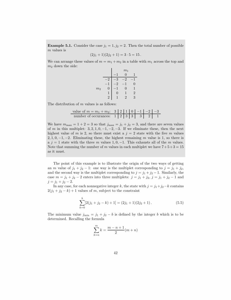
Example 5.1. Consider the case j1 = 1, j2 = 2. Then the total number of possiblem values is
(2j1 + 1)(2j2 + 1) = 3 · 5 = 15 .
We can arrange these values of m = m1 +m2 in a table with m1 across the top andm2 down the side:
m2
m1
−1 0 1−2 −3 −2 −1−1 −2 −1 0
0 −1 0 11 0 1 22 1 2 3
The distribution of m values is as follows:
value of m = m1 +m2: 3 2 1 0 −1 −2 −3number of occurances: 1 2 3 3 3 2 1
We have mmax = 1 + 2 = 3 so that jmax = j1 + j2 = 3, and there are seven valuesof m in this multiplet: 3, 2, 1, 0,−1,−2,−3. If we eliminate these, then the nexthighest value of m is 2, so there must exist a j = 2 state with the five m values2, 1, 0,−1,−2. Eliminating these, the highest remaining m value is 1, so there isa j = 1 state with the three m values 1, 0,−1. This exhausts all of the m values.Note that summing the number of m values in each multiplet we have 7+5+3 = 15as it must.
The point of this example is to illustrate the origin of the two ways of gettingan m value of j1 + j2 − 1: one way is the multiplet corresponding to j = j1 + j2,and the second way is the multiplet corresponding to j = j1 + j2 − 1. Similarly, thecase m = j1 + j2 − 2 enters into three multiplets: j = j1 + j2, j = j1 + j2 − 1 andj = j1 + j2 − 2.
In any case, for each nonnegative integer k, the state with j = j1+j2−k contains2(j1 + j2 − k) + 1 values of m, subject to the constraint
b∑
k=0
[2(j1 + j2 − k) + 1] = (2j1 + 1)(2j2 + 1) . (5.5)
The minimum value jmin = j1 + j2 − b is defined by the integer b which is to bedetermined. Recalling the formula
m∑
k=n
k =m− n+ 1
2(m+ n)
42
we have
b∑
k=0
[2(j1 + j2 − k) + 1] = 2(j1 + j2)(b + 1) − 2
b∑
k=0
k + (b + 1)
= 2(j1 + j2)(b + 1) − (b+ 1)b+ (b + 1)
= (b+ 1)[2(j1 + j2) + 1 − b] .
Then equation (5.5) becomes
(b + 1)[2(j1 + j2) + 1 − b] = (2j1 + 1)(2j2 + 1)
orb2 − 2(j1 + j2)b+ 4j1j2 = 0 .
Solving for b using the quadratic formula yields
b = (j1 + j2) ±√
(j1 + j2)2 − 4j1j2
= (j1 + j2) ± (j1 − j2)
so that b = 2j1 or b = 2j2. Since jmin = j1 + j2− b, we see that either jmin = j2− j1or jmin = j1 − j2. If j1 6= j2 then one of these is negative and must be rejected, andhence we conclude that jmin = |j1 − j2|. Thus we arrive at jmin ≤ j ≤ jmax or
|j1 − j2| ≤ j ≤ j1 + j2 . (5.6)
Equations (5.1c), (5.3), (5.4) and (5.6) are all we need to calculate the Clebsch-Gordan coefficients. The procedure is best illustrated by a specific example.
Example 5.2. Let us consider the case j1 = j2 = 1/2 because you (should) alreadyknow the answer. In this case we have m1 = m2 = ±1/2, so according to equation(5.6) we know that 0 ≤ j ≤ 1.
First we have jmax = j1 + j2 = 1, and the maximum value of m is m1 +m2 = 1also. From equation (5.3) we have the single term
∣∣∣1 1⟩
=∣∣∣1
2
1
2
⟩⟨1
2
1
2
∣∣∣1 1⟩
and by equation (5.4) we must have
∣∣∣∣⟨1
2
1
2
∣∣∣1 1⟩∣∣∣∣
2
= 1 .
This specifies the topmost state up to a phase factor. Choosing this phase to be 1(the Condon-Shortley convention), we are left with
⟨1
2
1
2
∣∣∣1 1⟩
= +1 .
43
Hence equation (5.3) becomes
∣∣∣1 1⟩
=∣∣∣1
2
1
2
⟩(5.7a)
where the state on the left-hand side of this equation is the |jm〉 state, and thestate on the right-hand side is the |m1m2〉 state.
To construct the next lowest state, we act on the left-hand side of this last resultwith J−, and on the right-hand side with J− = J1− + J2−. Using equation (5.1c),we obtain
√2∣∣∣1 0
⟩=
√3
4+
1
4
∣∣∣ − 1
2
1
2
⟩+
∣∣∣1
2− 1
2
⟩
or ∣∣∣1 0⟩
=1√2
∣∣∣ − 1
2
1
2
⟩+
∣∣∣1
2− 1
2
⟩. (5.7b)
Since (by equation (5.3))
∣∣∣1 0⟩
=∣∣∣1
2− 1
2
⟩⟨1
2− 1
2
∣∣∣1 0⟩
+∣∣∣ − 1
2
1
2
⟩⟨− 1
2
1
2
∣∣∣1 0⟩
we see that ⟨1
2− 1
2
∣∣∣1 0⟩
=⟨− 1
2
1
2
∣∣∣1 0⟩
=1√2.
We now act on equation (5.7b) with J− = J1− + J2− again to obtain
√2∣∣∣1 − 1
⟩=
1√2
[√3
4+
1
4
∣∣∣ − 1
2− 1
2
⟩+
∣∣∣ − 1
2− 1
2
⟩]
or ∣∣∣1 − 1⟩
=∣∣∣ − 1
2− 1
2
⟩(5.7c)
and hence ⟨− 1
2− 1
2
∣∣∣1 − 1⟩
= 1 .
This completes the j = 1 multiplet which, for obvious reasons, is called the triplet
state.Now for the j = 0 state. We know from equation (5.3) that
∣∣∣0 0⟩
=∣∣∣1
2− 1
2
⟩⟨1
2− 1
2
∣∣∣0 0⟩
+∣∣∣ − 1
2
1
2
⟩⟨− 1
2
1
2
∣∣∣0 0⟩
:=∣∣∣1
2− 1
2
⟩a+
∣∣∣ − 1
2
1
2
⟩b .
To solve for a and b, we first see that from equation (5.4) we have a2 + b2 = 1.Next, we note that the |jm〉 = |1 0〉 state is orthogonal to the |jm〉 = |0 0〉 state,and therefore
0 = 〈1 0|0 0〉 =1√2(a+ b)
44
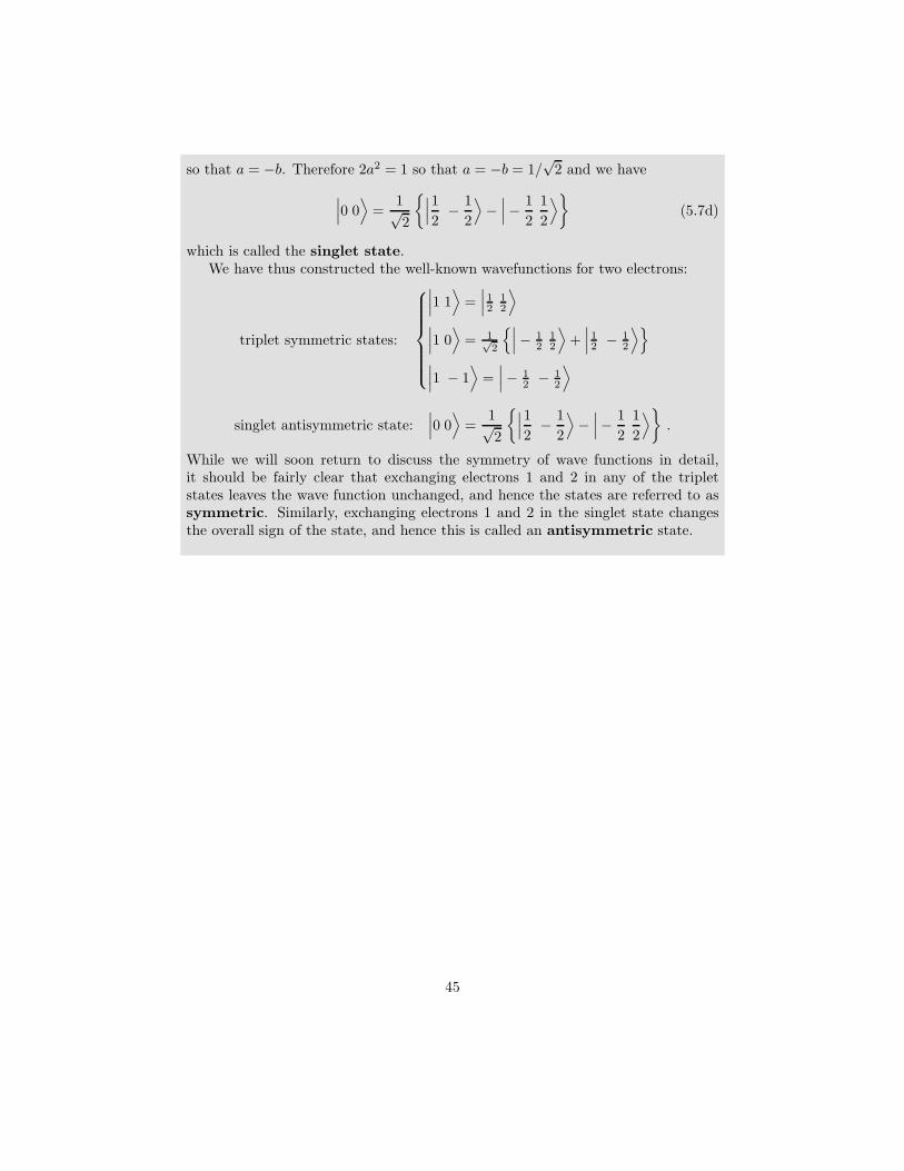
so that a = −b. Therefore 2a2 = 1 so that a = −b = 1/√
2 and we have
∣∣∣0 0⟩
=1√2
∣∣∣1
2− 1
2
⟩−
∣∣∣ − 1
2
1
2
⟩(5.7d)
which is called the singlet state.We have thus constructed the well-known wavefunctions for two electrons:
triplet symmetric states:
∣∣∣1 1⟩
=∣∣∣12
12
⟩
∣∣∣1 0⟩
= 1√2
∣∣∣ − 12
12
⟩+
∣∣∣12 − 1
2
⟩
∣∣∣1 − 1⟩
=∣∣∣ − 1
2 − 12
⟩
singlet antisymmetric state:∣∣∣0 0
⟩=
1√2
∣∣∣1
2− 1
2
⟩−
∣∣∣ − 1
2
1
2
⟩.
While we will soon return to discuss the symmetry of wave functions in detail,it should be fairly clear that exchanging electrons 1 and 2 in any of the tripletstates leaves the wave function unchanged, and hence the states are referred to assymmetric. Similarly, exchanging electrons 1 and 2 in the singlet state changesthe overall sign of the state, and hence this is called an antisymmetric state.
45