chapter 1-6 review
DESCRIPTION
Chapter 1-6 Review. Chapter 1. The mean, variance and minimizing error. = = 1.79. (X- ) = 0.00. (X- ) 2 = SS = 16.00. X = 30 N = 5 = 6.00. - PowerPoint PPT PresentationTRANSCRIPT
Chapter 1-6 Review

Chapter 1
• The mean, variance and minimizing error
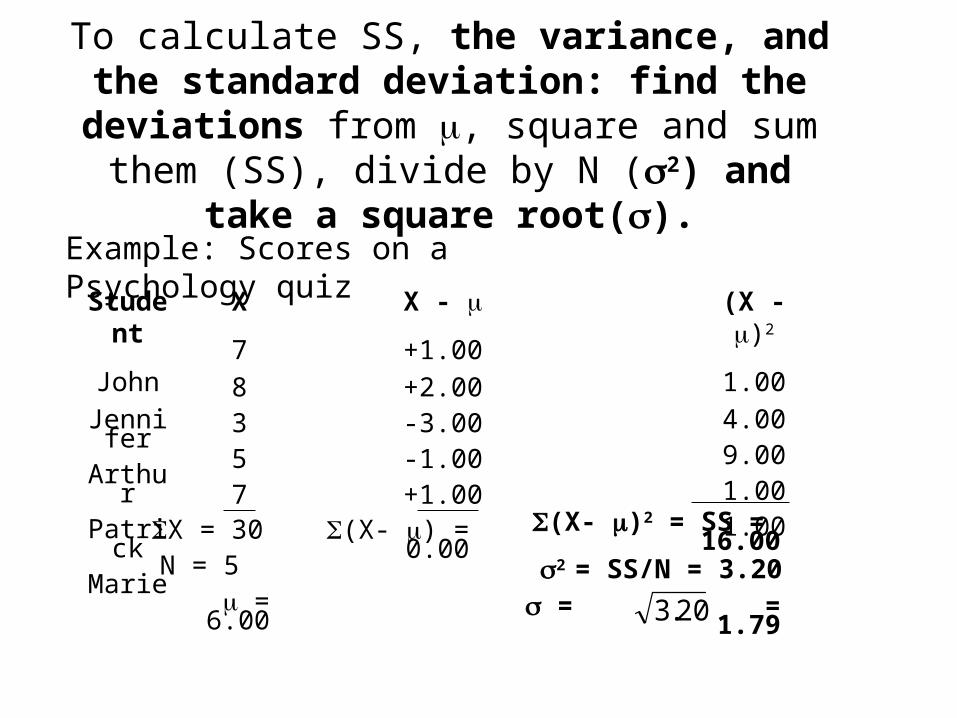
To calculate SS, the variance, and the standard deviation: find the deviations from , square and
sum them (SS), divide by N (2) and take a square root().
Example: Scores on a Psychology quiz
Student
John
JenniferArthurPatrickMarie
X
7
8357
X = 30 N = 5 = 6.00
X -
+1.00
+2.00-3.00-1.00+1.00
(X- ) = 0.00
(X - )2
1.00
4.009.001.001.00
(X- )2 = SS = 16.00
2 = SS/N = 3.20 = = 1.7920.3

If you must make a prediction of someone’s score, say everyone will score
precisely at the population mean, mu.
• Without any other information, the mean is the best prediction.
• The mean is an unbiased predictor or estimate, because the deviations around the mean sum to zero [(X- ) = 0.00].
• The mean is the smallest average squared distance from the other numbers in the distribution. So it is called a least squares predictor.

Error is the squared amount you are wrong
• When you predict that everyone will score at the mean, you are wrong.
• The amount you are wrong is the difference between each score and the mean (X- ).
• But in statistics, we square the amount that we are wrong when we measure error.
2 is precisely how much error we make, on the average, when we predict that everyone will score right at the mean.
• Another name for the variance (2) is the “mean square for error”.

Why doesn’t everyone score precisely at the mean?
• Two sources of error– Random individual differences– Random measurement problems
Because people will always be different from each other and there are always random measurement problems, there will always be some error inherent in our predictions.
Theoretical histograms

Rolling a die – Rectangular distributionThe mean provides no information
120 rolls - how many of each number do you expect?
1 2 3 4 5 6
100
75
50
25
0

Normal Curve

J Curve
Occurs when socially normative behaviors are measured.Most people follow the norm, but there are always a few outliers.

Principles of Theoretical Curves• Expected freq. = Theoretical relative frequency (N)
• Expected frequencies are your best estimates because they are closer, on the average, than any other estimate when we square the error.
• Law of Large Numbers - The more observations that we have, the closer the relative frequencies should come to the theoretical distribution.
The Normal Curve

The Z table and the curve• The Z table shows a cumulative relative frequency
distribution. • That is, the Z table lists the proportion of the area
under a normal curve between the mean and points further and further from the mean.
• Because the two sides of the normal curve areexactly the same, the Z table shows only the cumulative proportion in one half of the curve. The highest proportion possible on the Z table is therefore .5000

KEY CONCEPT
The proportion of the curve between any two points on the curve represents the relative frequency of scores between those points.

Normal CurveFrequency
Measure
The mean
The standard deviation
|------------------------------97.72--------------------------||--------47.72-----------|---------47.72--------|
-3.00 -2.00 -1.00 0.00 1.00 2.00 3.00Z scores
|---34.13--|--34.13---|Percentages
Percentiles
3 2 1 0 1 2 3Standard
deviations

Z scores
• A Z score indicates the position of a raw score in terms of standard deviations from the mean on the normal curve.
• In effect, Z scores convert any measure (inches, miles, milliseconds) to a standard measure of standard deviations.
• Z scores have a mean of 0 and a standard deviation of 1.

Calculating z scores
Z =score - mean
standard deviation
What is the Z score for someone 6’ tall, if the mean is 5’8” and the standard deviation is 3 inches?
Z =6’ - 5’8”
3”
=72 - 68
3 =
4
3 = 1.33

2100
2080 22802030 2330
ProductionFrequency
units
2180
What is the Z score for a daily production of 2100, given a mean of 2180 units and a standard deviation of 50 units?
Z score = ( 2100 - 2180) / 50
3 2 1 0 1 2 3Standard
deviations
= -80 / 50
= -1.60
22302130
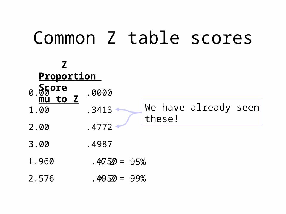
Common Z table scores
Z Proportion Score mu to Z
0.00 .0000
3.00 .4987
2.00 .4772
1.00 .3413
1.960 .4750
2.576 .4950 X 2 = 99%
X 2 = 95%
We have already seenthese!

CPE - 3.4 - Calculate percentiles
Z Area Add to .5000 (if Z > 0)Score mu to Z Sub from .5000 (if Z < 0) Proportion Percentile
-2.22 .4868 .5000 - .4868 .0132 1st
-0.68 .2517 .5000 - .2517 .2483 25th
+2.10 .4821 .5000 + .4821 .9821 98th
+0.33 .1293 .5000 + .1293 .6293 63rd
+0.00 .0000 .5000 + .0000 .5000 50th

-1.06
Proportion of scores between two points on opposite sides of the mean
Frequency
Percent between two scores.
-3.00 -2.00 -1.00 0.00 1.00 2.00 3.00Z scores
+0.37
Proportion mu to Z for -1.06= .3554
Proportion mu to Z for .37= .1443
Area Area Add/Sub Total Per Z1 Z2 mu to Z1 mu to Z2 Z1 to Z2 Area Cent
-1.06 +0.37 .3554 .1443 Add .4997 49.97 %

+1.50
Proportion of scores between two points on the same side of the mean
Frequency
Percent between two scores.
-3.00 -2.00 -1.00 0.00 1.00 2.00 3.00Z scores
+1.12
Proportion mu to Z for 1.12= .3686
Proportion mu to Z for 1.50= .4332
Area Area Add/Sub Total Per Z1 Z2 mu to Z1 mu to Z2 Z1 to Z2 Area Cent
+1.50 +1.12 .4332 .3686 Sub .0646 6.46 %

Translating to and from Z scores, the standard error of the mean
and confidence intervals

Definition
Z =score - mean
standard deviation
If we know mu and sigma, any score can be translated into a Z score:
=X -

DefinitionConversely, as long as you know mu and sigma, a Z score can be translated into any other type of score:
Score = + ( Z * )
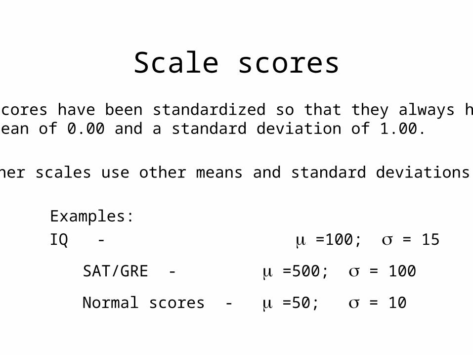
Scale scores
Z scores have been standardized so that they always have a mean of 0.00 and a standard deviation of 1.00.
Other scales use other means and standard deviations.
Examples:
IQ - =100; = 15
SAT/GRE - =500; = 100
Normal scores - =50; = 10

Convert Z scores to IQ scores
Z (Z*) + (Z * )
+2.67
-.060 15 -9.00 100 91
+2.67 15 40.05 +2.67 15 +2.67 15 40.05 100 +2.67 15 40.05 100 140

Translate to a Z score first, then to any
other type of score Convert IQ scores of 120 & 80 to percentiles.
120 100 20.0 15 1.33mu-Z = .4082, .5000 + .4082 = .9082 = 91st percentile, Similarly 80 = .5000 - .4082 = 9th percentile
X (X-) (X-)/
Convert an IQ score of 100 to a percentile.An IQ of 100 is right at the mean and that’s the 50th percentile.

SAT / GRE scores - Examples
How many people out of 400 can be expected to score between 550 and 650 on the SAT?
Proportion difference = .4332 - .1915 = .2417
550 500 50 100 0.50
SAT (X-) (X-)/
650 500 150 100 1.50 Proportion mu to Z0.50 = .1915
Proportion mu to Z1.50 = .4332
Expected people = .2417 * 400 = 96.68

Midterm type problems:Double translations
35 25.00 10.00 6.00 1.67
On the verbal portion of the Wechsler IQ test, John scores 35 correct responses. The mean on this part of the IQ test is 25.00 and the standard deviation is 6.00. What is John’s verbal IQ score?
Raw (X- ) Scale Scale Scale
score (raw) (raw) Z score
6.00 1.67 100 15 125
Scale score = 100 + (1.67 * 15) = 125
Z score = 10.00 / 6.00 = 1.67

The standard error = the standard deviation divided by the square
root of n, the sample size

Let’s see how it works• We know that the mean of SAT/GRE scores = 500 and sigma
= 100
• So 68.26% of individuals will score between 400 and 600 and 95.44% will score between 300 and 700
• But if we take random samples of SAT scores, with 4 people in each sample, the standard error of the mean is sigma divided by the square root of the sample size = 100/2=50.
• 68.26% of the sample means will be within 1.00 standard error of the mean from mu and 95.44% will be within 2.00 standard errors of the mean from mu
• So, 68.26% of the sample means (n=4) will be between 450 and 550 and 95.44% will fall between 400 and 600

What happens as n increases? • The sample means get closer to each other and to mu.• Their average squared distance from mu equals the
standard deviation divided by the size of the sample.• The law of large numbers operates – the pattern of
actual means approaches the theoretical frequency distribution. In this case, the sample means fall into a more and more perfect normal curve.
• These facts are called “The Central Limit Theorem” and can be proven mathematically.

Let’s make the samples larger• Take random samples of SAT scores, with 400 people in each sample, the
standard error of the mean is sigma divided by the square root of 400 = 100/20=5.00
• 68.26% of the sample means will be within 1.00 standard error of the mean from mu and 95.44% will be within 2.00 standard errors of the mean from mu.
• So, 68.26% of the sample means (n=400) will be between 495 and 505 and 95.44% will fall between 490 and 510.
• Take random samples of SAT scores, with 2500 people in each sample, the standard error of the mean is sigma divided by the square root of 2500 = 100/50=2.00.
• 68.26% of the sample means will be within 1.00 standard error of the mean from mu and 95.44% will be within 2.00 standard errors of the mean from mu.
• 68.26% of the sample means (n=2500) will be between 498 and 512 and 95.44% will fall between 496 and 504
CONFIDENCE INTERVALS

We want to define two intervals around mu:
One interval into which 95% of the sample means will fall.
Another interval into which 99% of the sample means will fall.

95% of sample means will fall in a symmetrical interval around mu that goes from 1.960 standard
errors below mu to 1.960 standard errors above mu
• A way to write that fact in statistical language is:
CI.95: mu + 1.960 sigmaX-bar or
CI.95: mu - 1.960 sigmaX-bar < X-bar < mu + 1.960 sigmaX-bar

As I said, 95% of sample means will fall in a symmetrical interval around mu that goes from 1.960
standard errors below mu to 1.960 standard errors above mu
• Take samples of SAT/GRE scores (n=400)
• Standard error of the mean is sigma divided by the square root of n=100/ = 100/20.00=5.00
• 1.960 standard errors of the mean with such samples = 1.960 (5.00)= 9.80
• So 95% of the sample means can be expected to fall in the interval 500+9.80
• 500-9.80 = 490.20 and 500+9.80 =509.80
CI.95: mu + 1.960 sigmaX-bar = 500+9.80 or
CI.95: 490.20 < X-bar < 509.20
400

99% of sample means will fall within 2.576 standard errors from mu
• Take the same samples of SAT/GRE scores (n=400)
• The standard error of the mean is sigma divided by the square root of n=100/20.00=5.00
• 2.576 standard errors of the mean with such samples =
2.576 (5.00)= 12.88
• So 99% of the sample means can be expected to fall in the interval 500+12.88
• 500-12.88 = 487.12 and 500+12.88 =512.88
CI.99: mu + 2.576 sigmaX-bar = 500+12.88 or
CI.99: 487.12 < X-bar < 512.88

Chapter 5-Samples

REPRESENTATIVE ON EVERY MEASURE
• The mean of the random sample will be similar to the mean of the population.
• The same holds for weight, IQ, ability to remember faces or numbers, the size of their livers, self-confidence, etc., etc., etc. ON EVERY MEASURE THAT EVER WAS OR CAN BE AND ON EVERY STATISTIC WE COMPUTE, SAMPLE STATISTICS ARE LEAST SQUARED, UNBIASED, CONSISTENT ESTIMATES OF THEIR POPULATION PARAMETERS.

The sample mean
The sample mean is called X-bar and is represented by X.
X is the best estimate of , because it is a leastsquares, unbiased, consistent estimate.
X = X / n

Consistent estimation
Population is 1320 students taking a test.
is 72.00, = 12
Let’s randomly sample one student at a time and see what happens.
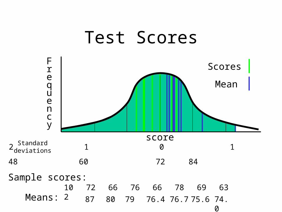
Test ScoresFrequency
score
36 48 60 96 10872 84
Sample scores:
3 2 1 0 1 2 3Standard
deviations
Scores
Mean
87Means: 80 79
102 72 66 76 66 78 69 63
76.4 76.7 75.6 74.0

More scores that are free to vary = better estimates
Each time you add a score to your sample, it is most likely to pull the sample mean closer to mu, the population mean.
Any particular score may pull it further from mu.
But, on the average, as you add more and more scores, the oddsare that you will be getting closer to mu..
Remember, if your sample was everybody in the population, then the sample mean must be exactly mu.

Consistent estimators
We call estimates that improve when you add scoresto the sample consistent estimators.
Recall that the statistics that we will learn are:consistent,least squares, andunbiased.

Estimated variance
Our best estimate of 2 is called the mean square for error and is represented by MSW.
MSW is a least squares, unbiased, consistentestimate.
SSW = (X - X)2
MSW = (X - X)2 / (n-k)
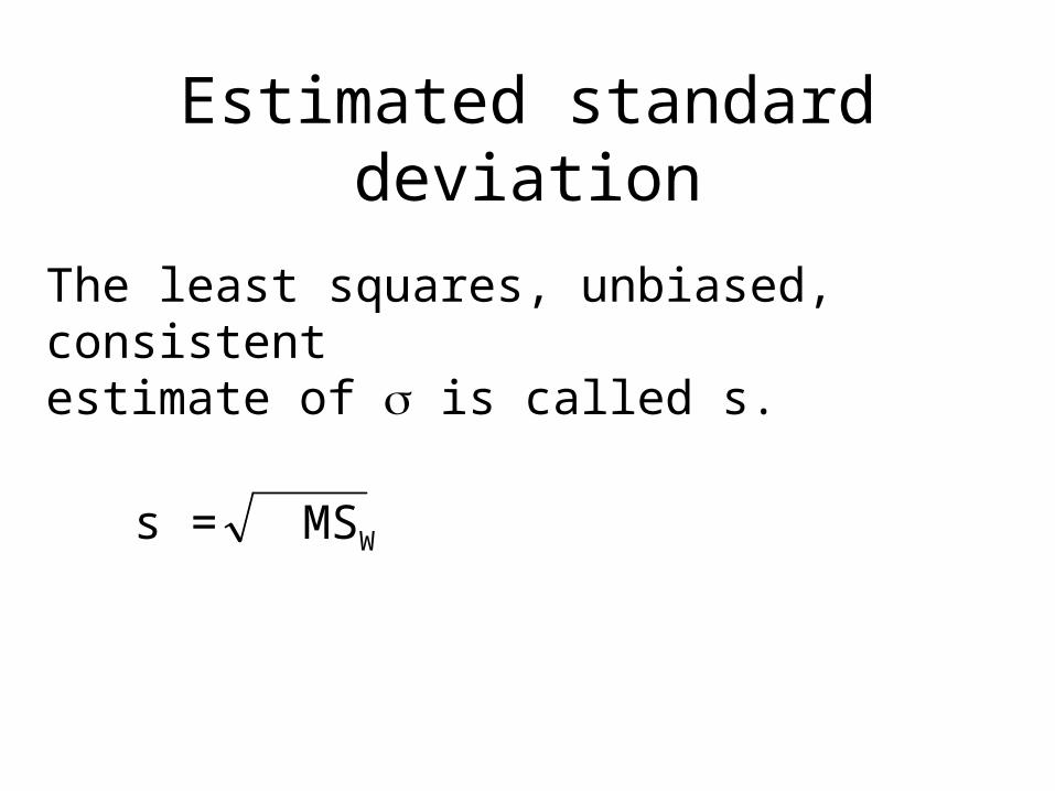
Estimated standard deviation
The least squares, unbiased, consistent estimate of is called s.
s = MSW

Estimating mu and sigma – single sample
S#ABC
X684
MSW = SSW/(n-k) = 8.00/2 = 4.00
s = MSW = 2.00
(X - X)2
0.00 4.004.00
(X - X) 0.00 2.00-2.00
X6.006.006.00
X=18 N= 3
X=6.00
(X-X)=0.00 (X-X)2=8.00 = SSW

Why n-k?
• This has to do with “degrees of freedom.”
• Each time you add a score to a sample, you pull the sample statistic toward the population parameter.

Any score that isn’t free to vary does not tend to pull the sample statistic toward the population parameter.
• When calculating the estimated average squared deviation from the mean, we base our estimate on the deviation of each score from its group mean.
• So there are as many df for MSW and s as there are deviation scores that are free to vary.
• One deviation in each group is constrained by the rule that deviations around the mean must sum to zero. So one score in each group is not free to vary.

Group11.11.21.31.4
X50776988
MSW = SSW/(n-k) =
s = MSW =
(X - X)2
441.0036.00
4.00289.00
(X - X) -21.00
+6.00-2.00
+17.00
(X-X1)=0.00 (X-X1)2= 770.00Group2
2.12.22.32.4
78578263
(X-X2)2= 426.00(X-X2)=0.00
64.00169.00144.0049.00
8.00-13.0012.00-7.00
Group33.13.23.33.4
74706381
X71.0071.0071.0071.00
X1 = 71.00
70.0070.0070.0070.00
X2 = 70.00
(X-X3)2= 170.00(X-X3)=0.00
4.004.00
81.0081.00
2.00-2.00-9.009.00
72.0072.0072.0072.00
X3 = 72.00
1366.00/9 = 151.78
151.78 = 12.32

n-k is the number of degrees of freedom for MSW
• Since one deviation score in each group is not free to vary, you lose one degree of freedom for each group - with k groups you lose k*1=k degrees of freedom.
• There are n deviation scores in total. k are not free to vary. That leaves n-k that are free to vary, n-k degrees of freedom MSW, your estimate of sigma2.

t distribution, estimated standard errors and CIs with t

t curves
• The more degrees of freedom for MSW, the better our estimate of sigma2.
• The better our estimate, the more t curves resemble Z curves.

1 df
To get 95% of the population when there is 1 df of freedom, you need to go out over 12 standard deviations.
5 df
To get 95% of the population when there are 5 df of freedom, you need to go out over 3 standard deviations.
t curves and degrees of freedomFrequency
score3 2 1 0 1 2 3
Standarddeviations

Critical values of the t curves• Each curve is defined by how many estimated
standard deviations you must go from the mean to define a symmetrical interval that contains a proportions of .9500 and .9900 of the curve, leaving proportions of .0500 and .0100 in the two tails of the curve (combined).
• Values for .9500/.0500 are shown in plain print. Values for .9900/.0100 and the degrees of freedom for each curve are shown in bold print.

df 1 2 3 4 5 6 7 8.05 12.706 4.303 3.182 2.776 2.571 2.447 2.365 2.306.01 63.657 9.925 5.841 4.604 4.032 3.707 3.499 3.355
df 9 10 11 12 13 14 15 16.05 2.262 2.228 2.201 2.179 2.160 2.145 2.131 2.120.01 3.250 3.169 3.106 3.055 3.012 2.997 2.947 2.921
df 17 18 19 20 21 22 23 24.05 2.110 2.101 2.093 2.086 2.080 2.074 2.069 2.064.01 2.898 2.878 2.861 2.845 2.831 2.819 2.807 2.797
df 25 26 27 28 29 30 40 60.05 2.060 2.056 2.052 2.048 2.045 2.042 2.021 2.000.01 2.787 2.779 2.771 2.763 2.756 2.750 2.704 2.660
df 100 200 500 1000 2000 10000.05 1.984 1.972 1.965 1.962 1.961 1.960.01 2.626 2.601 2.586 2.581 2.578 2.576
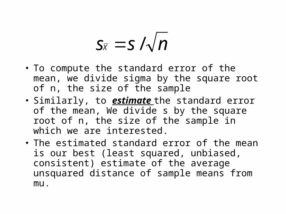
• To compute the standard error of the mean, we divide sigma by the square root of n, the size of the sample
• Similarly, to estimate the standard error of the mean, We divide s by the square root of n, the size of the sample in which we are interested.
• The estimated standard error of the mean is our best (least squared, unbiased, consistent) estimate of the average unsquared distance of sample means from mu.
nssX /

Confidence intervals around muT

Confidence intervals and hypothetical means
• We frequently have a theory about what the mean of a distribution should be.
• To be scientific, that theory about mu must be able to be proved wrong (falsified).
• One way to test a theory about a mean is to state a range where sample means should fall if the theory is correct.
• We usually state that range as a 95% confidence interval.

• To test our theory, we take a random sample from the appropriate population and see if the sample mean falls where the theory says it should, inside the confidence interval.
• If the sample mean falls outside the 95% confidence interval established by the theory, the evidence suggests that our theoretical population mean and the theory that led to its prediction is wrong.
• When that happens our theory has been falsified. We must discard it and look for an alternative explanation of our data.

Testing a theory• SO WE MUST CONSTRUCT A 95% CONFIDENCE
INTERVAL AROUND MUT AND SEE WHETHER OUR SAMPLE MEAN FALLS INSIDE OR OUTSIDE THE CI.
• If the sample mean falls inside the CI.95, you must accept muT as the most probable mean for the population from which the sample was drawn.
• If the sample means falls outside the CI.95, you falsify the theory that the population mean equals muT. You then turn around and ask what the relevant population parameter is. And there is the sample mean, a least squares, unbiased estimate of mu. If the mean is not muT, then we use the sample mean as our estimate of mu.

To create a confidence interval around muT, we must estimate sigma from a sample.
• For example, we randomly select a group of 16 healthy individuals from the population.
• We administer a standard clinical dose of our new drug for 3 days.
• We carefully measure body temperature.• RESULTS: We find that the average body
temperature in our sample is 99.5oF with an estimated standard deviation of 1.40o (s=1.40).
• IS 99.5oF. IN THE 95% CI AROUND MUT???

Knowing s and n we can easily compute the estimated standard error of the mean.
• Let’s say that s=1.40o and n = 16:
• = 1.40/4.00 = 0.35nssX /

df 1 2 3 4 5 6 7 8.05 12.706 4.303 3.182 2.776 2.571 2.447 2.365 2.306.01 63.657 9.925 5.841 4.604 4.032 3.707 3.499 3.355
df 9 10 11 12 13 14 15 16
.05 2.262 2.228 2.201 2.179 2.160 2.145 2.131 2.120
.01 3.250 3.169 3.106 3.055 3.012 2.997 2.947 2.921
df 17 18 19 20 21 22 23 24.05 2.110 2.101 2.093 2.086 2.080 2.074 2.069 2.064.01 2.898 2.878 2.861 2.845 2.831 2.819 2.807 2.797
df 25 26 27 28 29 30 40 60.05 2.060 2.056 2.052 2.048 2.045 2.042 2.021 2.000.01 2.787 2.779 2.771 2.763 2.756 2.750 2.704 2.660
df 100 200 500 1000 2000 10000.05 1.984 1.972 1.965 1.962 1.961 1.960.01 2.626 2.601 2.586 2.581 2.578 2.576

So, muT=98.6, dfW=15, tCRIT=2.131, s=1.40, n=16, sX-bar=1.40/ = 0.35
Here is the confidence intervalCI.95: muT + tCRIT* sX-bar =
= 98.6 + (2.131)(0.35) = 98.60+ 0.75
CI.95: 97.85 < X-bar < 99.35
Our sample mean (99.5) fell outside the CI.95 This falsifies the theory that our drug has no effect on body temperature. Our drug may cause a slight fever.
16