cereal consumption and per capita income in india

SPECIAL ARTICLE

Economic & Political Weekly EPW FEBRuary 11, 2012 vol xlvii no 6 63

Cereal Consumption and Per Capita Income in India

Christian Oldiges

This paper examines the relationship between per capita

cereal consumption and per capita income in India using

the India Human Development Survey 2004-05. It turns

out that per capita cereal consumption remains much

the same at different levels of per capita income, though

it does vary substantially with education levels, household

size, occupation patterns and urbanisation. The recent

decline of cereal consumption over time may reflect

changes in these non-income factors. While cereal

consumption seems unrelated to per capita income, it is

positively related to per capita expenditure. Possible

interpretations of this contrast are briefly discussed.

I am very grateful to Jean Drèze for guidance and innumerable suggestions. I also want to thank Carsten Bormann, Vanita Leah Falcao, Aashish Gupta, Reetika Khera and Stefan Klonner for very helpful advice, and Allahabad University for logistic support.

Christian Oldiges ([email protected]) is pursuing a PhD in Development Economics at Heidelberg University, Germany.

1 Introduction

In India, per capita cereal consumption (PCCC) is often meas-ured against monthly per capita consumption expenditure (MPCE). Based on National Sample Survey (NSS) data, the

relationship between the two is a little puzzling: in any given year, PCCC is positively related to MPCE across households, but over time, PCCC has been declining in spite of a sustained rise in MPCE.1 In other words, there is a contrast between cross-section and time series data on the relation between PCCC and MPCE. The positive relation between the two in cross-section data also contrasts to some extent with international cross-sec-tion patterns: across countries, PCCC is lower at higher levels of per capita expenditure.

This paper extends the evidence by examining the relation-ship between PCCC and per capita income (PCI) in a given year. Household surveys like the NSS collect consumption expendi-ture data but no income data. The India Human Development Survey (IHDS), however, collected both income and consump-tion expenditure data in 2004-05, enabling us to look at both income and expenditure elasticities of PCCC in 2004-05.2

Our main finding is that PCCC remains much the same at different levels of PCI (within rural or urban areas). In rural areas, for instance, PCCC hovers around 12 kg per month across all income groups. This pattern contrasts sharply with positive income elasticities of demand for other food items such as milk, vegetables and fruits. Instead of being corre-lated with income, PCCC is substantially affected by educa-tional levels, household size and occupation patterns. After controlling for PCI, MPCE and other socio-economic variables, PCCC also varies across states and may therefore be influ-enced by regional food habits and local preferences.

This does not mean that there is a contradiction between NSS and IHDS data. Indeed, the positive relationship between PCCC and MPCE is also visible in the IHDS data and is very simi-lar to the corresponding relationship in NSS data. The real con-trast therefore is not between NSS and IHDS data but between expenditure-based and income-based Engel curves.

Recent research on changes in food consumption behaviour in India has been concerned with the decline of PCCC over the last few decades. In this context, the decline of PCCC has been attri buted to a diversification of diets (Dyson and Hanchate 2000), a higher availability of urban goods in rural areas (Kumar et al 2007), rising relative prices of cereals vis-à-vis other food items (Mittal 2007) and improved transport infrastructure (Rao 2000). Overall, researchers tend to argue that the decline in PCCC is related to development and increases in MPCE which enable households to move away from cereals towards a more

SPECIAL ARTICLE

FEBRuary 11, 2012 vol xlvii no 6 EPW Economic & Political Weekly64

diversified diet (Kumar et al 2009). However, this interpreta-tion appears to jar with the fact that PCCC is positively related to MPCE across households, so that an increase in MPCE would be expected to lead to an increase, not decline, in PCCC.

The findings of this paper suggest a somewhat modified reading of the evidence, whereby per capita income is not one of the main determinants of PCCC. Rather, PCCC depends mainly on factors such as education, occupation, region and food habits. The decline of PCCC over time possibly reflects changes in these factors including changes in occupational patterns and activity levels. The positive relation between PCCC and MPCE at a given point of time, for its part, appears to be driven by measurement errors or short-term (e g, seasonal) fluctuations in earnings, activity levels and energy requirements.

The remainder of the paper is divided into seven sections. Section 2 introduces to the two surveys (NSS and IHDS) and dis-cusses the data. In Section 3 data from the NSS and the IHDS sur-veys are used to examine the relationship between PCCC and MPCE in rural areas. Section 4 compares expenditure-based and income-based Engel-curves from IHDS data. In Section 5 these relationships are re-examined in a multivariate framework. Section 6 presents a summary of the corresponding findings for urban India (all data presented before that section pertain to rural areas, unless stated otherwise). Section 7 concludes.

2 NSS and IHDS

The main source of NSS data used in this paper is Report No 508 (“Household Consumer Expenditure Survey”) based on the NSS 61st round, conducted across the country between July 2004 and June 2005. Data were collected from a sample of 79,298 rural and 45,346 urban households spread over 7,999 villages and 4,602 urban blocks, respectively (NSSO 2006). In comparison, the IHDS sample consists of only 27,010 rural and 13,126 urban households, covering “all states and union terri-tories of India (with the exception of Andaman and Nicobar and Lakshadweep)”. Furthermore, “of the 612 districts in India in 2001, 382 are included in IHDS” and “the sample is spread across 1,503 villages and 971 urban blocks” (Desai et al 2010).

The National Sample Survey Office (NSSO) has been carry-ing out surveys over the last 60 years. It is the most established data collection organisation in India. The IHDS, on the other hand, is the first survey of its kind and requires some scrutiny. From Table 1, which compares IHDS data with data from the Census 2001, the NSS and the third National Family Health Survey (NFHS-3, conducted in 2005-06), IHDS ap-pears to be reasonably consistent with other sources. The selected indicators are meant to capture diverse fields related to

community, health and education taken from a larger list com-piled by Desai et al (2010).

Much of the analysis in this paper focuses on three variables – PCCC, MPCE and PCI. The main variable of interest is monthly PCCC, defined in both surveys as cereal consumption during the preceding 30 days. NSS reports include monthly PCCC (measured in kg) as “total cereals” which is the sum of rice, wheat, jowar, bajra, maize, barley, small millets, ragi and “other cereals”. Rice and wheat alone account for about 90% of total cereals. Monthly PCCC (measured in kg) is calculated from the IHDS data set as the sum of three items – wheat, rice and “other cereals”.

The NSS defines MPCE “for the household as the total con-sumer expenditure over all items divided by its size and ex-pressed on a per month (30 days) basis” (NSSO 2006: 5). In the NSS, household consumer expenditure pertains to “the total of the monetary values of consumption of various groups of items, namely, (1) food, paan (betel leaves), tobacco, intoxicants and fuel and light, (2) clothing and footwear, and (3) miscellane-ous goods and services and durable articles” (ibid: 4).3

The IHDS, on the other hand, measures MPCE on a mixed recall period. Questions regarding consumption expenditure “were modelled on the short form of the National Sample Survey” and data collection used “a mixed recall period with data for commonly used items restricted to the preceding 30 days” (Desai et al 2010).

In contrast, income data were collected for the preceding year. “The IHDS measure of income is summed across over 50 separate components including wages and salaries, net farm income, family business net income, property, and pension in-comes”. Total household income measured by the IHDS pertains to the entire year. In this paper, PCI refers to annual per capita income as calculated from IHDS data, expressed in rupees per month (for comparability with MPCE).

3 Per Capita Cereal Consumption and Expenditure

3.1 Evidence from NSS

Starting with NSS data, Table 2 illustrates PCCC trends over the last decades. While in the early 1970s monthly PCCC was as high as 15 kg or so, by 2007-08 it had declined by more than 20% to less than 12 kg. The decline has been steady over the years from the late 1970s onwards.

However, the decline in PCCC has not been homo-geneous across levels of MPCE. Table 3 gives PCCC

Table 1: Comparison of IHDS Data with Other Sources (in %) IHDS2004-05 NFHS2005-06 NSS2004-05 Census2001

SC population 21 19 20 16

ST population 7 8 9 8

Literacy rate, age 7 and above 68 69 67 65

Knowledge of AIDS 54 61 NA NA

Households with electricity 72 68 65 56Sources: Desai et al (2010, Table AI.3). SC: scheduled caste, ST: scheduled tribe.

Table 2: Per Capita Cereal Consumption in Rural India (1970-2008; kg/month)Year PCCC Year PCCC

1970 -71 15.35 1989-90 14.00

1972 -73 15.26 1990-91 14.06

1973 -74 15.09 1991-92 13.50

1977-78 15.25 1993-94 13.40

1983 14.80 1999-2000 12.72

1986-87 14.28 2004-05 12.11

1987-88 14.47 2007-08 11.76Source: Various NSS reports available at http://mospi.gov.in

Table 3: PCCC for Each MPCE Class (Rural India, 1993-2005; kg/month) 0-5 5-10 10-20 20-30 30-40 40-50 50-60 60-70 70-80 80-90 90-95 95-100

1993-94 9.68 11.29 12.03 12.63 13.19 13.33 13.72 14.07 14.41 14.59 14.98 15.78

1999-2000 9.78 11.15 11.64 12.27 12.56 12.89 13.03 13.36 13.45 13.67 13.73 14.19

2004-05 9.88 10.87 11.33 11.70 11.98 12.16 12.37 12.61 12.77 12.72 12.77 13.50

% change 1993-2005 2.1 -3.7 -5.8 -7.4 -9.2 -8.8 -9.8 -10.4 -11.4 -12.8 -14.8 -14.4

Source: NSS Report No 508. The column headings give the percentile range of the relevant MPCE class, from the poorest 5% to the top 5%.

SPECIAL ARTICLE


figures across 12 MPCE classes for the three “thick rounds” of the NSS between 1993-94 and 2004-05. The largest decline in PCCC occurred among the top MPCE classes, with reductions of up to 15%. In fact, the higher the MPCE class, the larger is the percentage decline. Figure 1 plots Engel curves based on Table 3. The basic pattern is a clockwise “swing” over time, with larger PCCC declines for higher MPCE classes.

Another pattern which emerges, to be compared with the income approach later on, is the relation between PCCC and MPCE at a point of time, i e, in a given year. One finds that PCCC increases across the 12 MPCE classes (Figure 1 and Table 3), hence a positive relationship in every year.

To sum up, two key findings emerge from NSS data. First, there is a positive and monotonic relationship between MPCE and PCCC across households; in other words, better-off households (in terms of MPCE) consume more cereals than poorer households. Sec-ond, over the last decades of rising MPCE levels, PCCC has de-clined, particularly (but not only) among higher MPCE classes.

3.2 Evidence from NSS and IHDS

It is now possible to compare the NSS 2004-05 findings with IHDS data for the same year. As Table 4 indicates, both surveys show a clear pattern of rising PCCC with higher expenditure levels. The relationship be-tween PCCC and MPCE is quite similar in both surveys, with, if anything, a somewhat higher expenditure elasticity of PCCC in the IHDS data.

4 Per Capita Cereal Consumption and Income

As mentioned earlier, the IHDS data set includes the per capita income, which provides a unique opportunity to analyse cereal consumption from an-other angle. In this section, IHDS data are used to compare expenditure-based with in-come-based variations in PCCC.

Table 5 presents a broad-brush picture of the PCCC-PCI relationship. Clearly, there is no positive relationship between PCCC and PCI, as observed

earlier between PCCC and MPCE. Indeed, there is hardly any change in PCCC across income classes. For the bottom decile, PCCC is 12.29 kg per month, just about 1% more than the 12.12 kg for the top quartile.

4.1 Comparison of Engel Curves The contrast discussed in the preceding section can also be seen (more clearly) by looking at MPCE-based and PCI-based Engel curves of per capita cereal consumption. These Engel curves, estimated by non-parametric methods from IHDS data, are plotted together in Figure 2.4 As expected, the MPCE-based Engel curve has a positive slope, relatively steep initially, and then gradually flattening. In contrast, the PCI-based Engel curve is more or less flat.

This pattern (a flat PCI-based Engel curve for cereals) con-trasts sharply with positive income elasticities of demand for milk, vegetables and fruits. Note also that cereal expenditure rises with per capita income, even though cereal consumption (in quantity terms) does not. This is because higher-income households tend to purchase more expensive cereals.

4.2 Interpretation

The question why the two approaches (MPCE-based and PCI-based) yield such different Engel curves (Figure 2) remains. One may recall that the IHDS collected income data on a yearly basis, whereas expenditure data are based on a monthly recall period. It is a common practice of national survey organisa-tions to collect expenditure rather than income data for the simple reason that total household income is difficult to measure. In rural India individuals often do not have regular occupa-tions or permanent jobs. Therefore, total household income cannot be traced back to one income source alone, but needs to be derived from several sources which may vary seasonally. Because of the diversity of income sources and the irregular flow of income, it is difficult to measure income as accurately as monthly consumption expenditure.

In light of this, analysing the relationship between PCCC and PCI may seem implausible. If PCI were so badly measured as to be virtually random, the flat PCI-based Engel curve would simply reflect measurement errors. However, it can be shown that the IHDS’ PCI variable is not just a random variable. Indeed,

Figure 1: Per Capita Cereal Consumption for MPCE Classes (1993-2005, Rural India)

Per C

apit

a C

erea

l Con

sum

pti

on

MPCE classes (%)

9

11

13

15

17

5 10 20 30 40 50 60 70 80 95 100

1993-94

1999-2000

2004-05

Source: See Table 3.

Table 4: PCCC for MPCE Classes (Rural India, 2004-05; kg/month) NSS IHDS

0-5 9.88 9.35

5-10 10.87 10.18

10-20 11.33 10.83

20-30 11.70 11.64

30-40 11.98 11.95

40-50 12.16 12.29

50-60 12.37 12.80

60-70 12.61 12.71

70-80 12.77 12.92

80-90 12.72 13.37

90-95 12.77 13.68

95-100 13.50 14.58Source: NSS Report No 508 and author’s calculations from IHDS data.

Table 5: PCCC for PCI Classes (Rural India, 2004-05; kg/month)

Bottom decile 12.29

Bottom quartile 12.10

Second quartile 12.09

Third quartile 12.21

Top quartile 12.12

Full sample 12.13Source: Author’s calculations from IHDS data.

Per C

apit

a C

erea

l Con

sum

pti

on

50

40

30

20

10

0

0 500 1,000 1,500 2,000Per capita income/per capita expenditure

Kernel = epanechnikov, degree = 0, bandwidth = 47.96Source: Author’s calculation from IHDS data. Q1, Q2, etc, indicate different quartiles of the per capita income scale. The diagram is restricted to per capita incomes below Rs 2,000, which include 90% of the observations.

Figure 2: PCI-Based and MPCE-Based Engel Curves (Rural India, 2004-05)

MPCE-based

PCI-based

SPECIAL ARTICLE


it correlates very well, in the expected manner, with other socio-economic variables such as education, occupation, and so on. This would not be the case if PCI were just “noise”.

PCCC and MPCE, too, are exposed to measurement errors, and further, PCCC measurement errors and MPCE measurement errors are likely to be correlated, because MPCE is the sum of cereal expenditure and other expenditure. According to Dea-ton and Subramaniam (1996), each item of consumption “is certainly measured with some error” and since MPCE is the sum of many different items, including cereals, MPCE is also measured with error. While calculating the Engel curve for PCCC with respect to MPCE, spurious correlation occurs as “the error of measurement is positively correlated with the compos-ite error term in the regression, itself partly determined by the measurement error in (cereals)”. As the lowest expenditure classes spend up to 35% on cereals (NSS Report No 508), this bias can be substantial, possibly reflected in the positive slope of the PCCC-MPCE curve.

The different slopes of the two Engel curves (MPCE-based and PCI-based) can also be plausibly related to the fact that con-sumption expenditure is measured on a monthly basis while in-come is measured on a yearly basis. Expenditure being month-based may entail that PCCC with respect to MPCE is exposed to the monthly fluctuations of expenditure. For instance, fluctua-tions can occur with seasonality. In harvest seasons, there is more work for agricultural labourers than in slack seasons. Be-sides more income at their disposal individuals are likely to have higher energy requirements in those seasons, resulting in higher cereal consumption. This, in turn, leads to a positive slope for the MPCE-based Engel curve.

Monthly expenditure is also exposed to fluctuations arising from short-term adjustments in consumption. Certain months may require a tightening of the belt due to unforeseen events like crop failure, death or sickness, etc. Especially poor house-holds who are not able to fall back on savings may then be forced to substantially adjust their consumption patterns. As other items of the household budget, e g, school fees, transport expenses or house rent may be difficult to adjust, alterations in cereal consumption may be the outcome. These could be reflected in a short-term response of PCCC to MPCE even if there is no relation between PCCC and per capita income on a yearly basis.

To illustrate the point, consider two identical agricultural labour households who are surveyed in different months, say one in the peak season and the other in the lean season. Even though their yearly income would be identical (by assump-tion), total consumption expenditure and PCCC would be re-ported as low for the household interviewed in the lean season and high for the other one. Hence, a positive relation between PCCC and MPCE would emerge.

4.3 Other Observations

This section supplements the preceding analysis with brief observations on the relationship between PCCC and various socio-economic indicators.

Dalit (or scheduled caste) and adivasi (or scheduled tribe) communities are among the most deprived in rural India.

Since NSS data suggest a positive relation between PCCC and MPCE, one would expect dalit and adivasi households to consume less cereals than the more affluent castes. Table 6, however, suggests that there are, in fact, no signifi-cant differences in PCCC across castes and religious groups. This is in line with the absence of any rela-tionship between PCCC and PCI (and with the pro-posed interpretations of this pattern, discussed in the preceding section).

It is another story, how-ever, when one considers occupation groups with their respective activity levels and energy require-ments. Table 7 shows average PCCC and PCI for different occu pation groups, and suggests that those with occupations in-volving manual labour consume more cereals than salaried or sedentary workers (Figure 3). That activity levels can play a role in determining cereal consump-tion has been discussed earlier by Deaton and Subramaniam (1996) and Deaton and Drèze (2009), among others. It is plau-sible enough that cereals act as a source of inexpensive calo-ries for workers engaged in heavy labour, with low wages but high calorie requirements.

Geographic differences in PCCC are also apparent, as illus-trated in Figure 4 (p 67). From these substantial interstate dif-ferences it appears at first sight that poorer states have higher PCCC levels than richer states (also see Appendix Table A1, p 71). For example, Bihar with a mean PCI of Rs 408 and mean PCCC of 16.08 kg contrasts with Kerala where PCI is about four times as high and PCCC (8.24 kg) about half as much. This relation-ship, however, is weakened by a few states like Himachal Pradesh with relatively high levels of PCI and PCCC, and

Table 6: Per Capita Cereal Consumption and Monthly Per Capita Income by Caste/Religious Group (Rural India, 2004-05; kg/month)Caste/Religion PCCC PCI

High caste 11.83 888

OBC 12.28 614

Dalit 12.26 499

Adivasi 12.18 534

Muslim 12.2 588

Other 10 1807OBC is Other Backward Classes.Source: Author’s calculation from IHDS data.

Table 7: Per Capita Cereal Consumption and Per Capita Income by Occupation Group (Rural India, 2004-05) Occupation PCCC PCI

Cultivation 12.63 634

Agriculture 12.07 416

Non-agri labour 12.06 449

Profession/pension 11.95 1,084

Salaried 11.70 1,182

Artisan 11.62 769

Other 11.54 684

Business 11.33 1,000

Petty trade 11.19 695

Total 12.13 646Source: Author’s calculations from IHDS data. Occupations (“main source of income”) are ranked in descending order of PCCC.

Figure 3: Per Capita Cereal Consumption and Per Capita Income by Occupation (Rural India, 2004-05)

Cultivation

Allied agAg labour

Non ag labour Artisan

Petty TradeBusiness

Salaried

Profession

Pension

8

10

12

14

200 400 600 800 1000 1200 1400

PC C

erea

l Con

sum

pti

on

200 400 600 800 1,000 1,200 1,400

14

12

10

8

Per capita incomeSource: Author’s calculations from IHDS data.

SPECIAL ARTICLE


and even significant in some cases. But this is a matter of spec-ification: the sign of the PCI co-variable can easily be made to “switch” from positive to negative or vice versa, by altering the list of independent variables (Figure 3 is one illustration of how the relation between PCI and PCCC can be made to “look” negative). This is an interesting example of how a spurious “significant” relationship (positive or negative, as desired) between two variables can easily be produced by suitable fiddling with the regression equation, when the two are actu-ally independent of each other. This is possible because the coefficient is close to zero.

In the regressions with MPCE as an independent variable, the coefficient for MPCE is always significant and positive. Despite this positive correlation, which is in line with the previous analysis, an elasticity of 0.06 indicates that the effect of MPCE on PCCC is quite small when other factors are controlled for.

Several other indicators seem to exert a greater influence on PCCC. Except for the coefficients for caste/religious group and ration card type, the results of the six regressions do not vary much in magnitude and significance. Overall, however, the first three regressions are explaining more of the variations in PCCC, mainly because state dummies are included. These state dum-mies are important to control for statewise differences in food habits, preferences and markets. The subsequent discussion, therefore, pertains to regression (1), unless stated otherwise.

The independent variables include two demographic indica-tors: child-person ratio and household size. The coefficient of the child-person ratio is negative and significant, as one would expect since children consume less than adults. The coefficient of household size is also significant and negative: at a given level of per capita income or per capita expenditure, per capita

Table 8: Definitions and Mean Values of Variables (Rural India, 2004-05)Variable Definition Mean

PCCC Per capita cereal consumption (kg/month) 12.56

PCI Per capita income (Rs/month) 666

MPCE Monthly per capita expenditure (Rs) 746

Household size Total number of persons in a household 5.66

Child-person ratio Individuals below age 21 per person in a household (%) 43

Education F Highest years of schooling of a female household member 3.27

Education M Highest years of schooling of a male household member 6.06

High Caste Dummy for high castes 0.17

OBC Dummy for other backward castes 0.37

Dalit Dummy for dalits 0.24

Adivasi Dummy for adivasis 0.1

Muslim Dummy for muslims 0.1

Other Dummy for other castes/religious groups 0.02

BPL Dummy for households with BPL card 0.36

Antyodaya Dummy for households with Antyodaya card 0.03

Cultivation Dummy for cultivation as main income source 0.35

Agriculture Dummy for agricultural labour as main income source 0.2

Non-agri labour Dummy for non-agricultural labour as main income source 0.17

Artisan Dummy for artisan as main income source 0.49

Petty Trade Dummy for petty trade as main income source 0.31

Business Dummy for business as main income source 0.35

Salaried Dummy for salaried as main income source 0.97

Profession/pension Dummy for profession/pension as main income source 0.29

Other Dummy for other income source 0.29Source: Author’s calculations from IHDS data. Jharkhand with low levels of PCI and PCCC. It seems that the

interstate patterns may be as much a matter of geography and food habits as a matter of development or per capita income.

5 Regression Analysis

5.1 Framework

So far we have looked at the relationship between PCCC and PCI (or MPCE) in a bivariate framework. In this section, differ-ent socio-economic, demographic and geographic indicators are included as independent variables in a simple linear re-gression model. The Ordinary Least Squares (OLS) estimation is based on the following equation:

yi = β0 + β'i Xi + εi,

where yi (the dependent variable) is PCCC for household i, β'i is a vector of coefficients, and Xi is a vector of independent variables including PCI and/or MPCE as well as indicators for demography (household size and child-adult ratio), education (years of schooling), occupation, caste or religious group, ration card type and location (state). The definition and mean value of each variable is given in Table 8. Regressions are run both with state dummies (regressions (1)-(3) in Table 9A, p 68) and without state-dummies (regressions (4)-(6)), and control for PCI and MPCE separately as well as simultaneously.

5.2 Main Findings

Table 9A presents the main findings of the six regressions, con-firming several of the earlier observations.

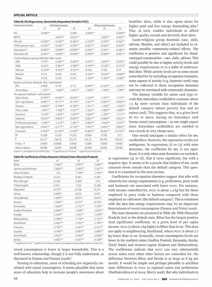
As expected, the coefficient of PCI is very close to zero (and this is a robust result). In most of the regressions presented in Table 9A, this close-to-zero coefficient happens to be positive,

Figure 4: Statewise Means of PCCC

Source: Author’s calculations from IHDS data.

14-17

13-14

12-13

10.5-12

0-10-5

Missing

PCCC (kg/month)

SPECIAL ARTICLE


cereal consumption is lower in larger households. This is a well-known relationship, though it is not fully understood, as discussed in Deaton and Paxson (1998).5

Turning to education, years of schooling are negatively cor-related with cereal consumption. It seems plausible that more years of education help to increase people’s awareness about

healthier diets, while it also opens doors for higher paid and less energy demanding jobs.6 This, in turn, enables individuals to afford higher quality cereals and diversify their diets.

Caste/religious group dummies (OBC, dalit, adivasi, Muslim, and other) are included to ex-amine possible community-related effects. The coefficient is positive and significant for disad-vantaged communities – OBC, dalit, adivasi. This could possibly be due to higher activity levels and energy requirements or to a habit of undiversi-fied diets. While activity levels are to some extent controlled for by including occupation dummies, some aspects of activity (e g, domestic work) may not be reflected in these occupation dummies and may be correlated with community dummies.

The dummy variable for ration card type re-veals that Antyodaya cardholders consume about 1.3 kg more cereals than individuals of the default category (above poverty line and no ration card). This suggests that, at a given level of PCI or MPCE, having an Antyodaya card boosts cereal consumption – as one might expect since Antyodaya cardholders are entitled to PDS cereals at very cheap rates.

One would anticipate a similar effect for BPL cardholders. However, the regression results are ambiguous. In regressions (1) to (3) with state dummies, the coefficient for BPL is not signi-ficant. It is only when state dummies are excluded,

in regressions (4) to (6), that it turns significant, but with a negative sign. It seems to be a puzzle that holders of BPL cards consume fewer cereals than the default category. This ques-tion is re-examined in the next section.

Coefficients for occupation dummies suggest that jobs with relatively low energy requirements (e g, professions, petty trade and business) are associated with lower PCCC. For instance, with income controlled for, PCCC is about 1.4 kg less for those employed in petty trade or business compared with those employed as cultivators (the default category). This is consistent with the idea that energy requirements may be an important determinant of cereal consumption (Deaton and Drèze 2009).

The state dummies are presented in Table 9B. With Himachal Pradesh (HP) as the default state, Bihar has the largest positive (and significant) coefficient. At a given level of per capita income, PCCC is about 3 kg higher in Bihar than in HP. This does not apply to neighbouring Jharkhand, where PCCC is about 2.7 kg lower than in HP. Generally, cereal consumption levels are lower in the southern states (Andhra Pradesh, Karnataka, Kerala, Tamil Nadu) and western region (Gujarat and Maharashtra). The coefficients indicate that PCCC can vary substantially across states even when other factors are controlled for: the difference between Bihar and Kerala is as large as 8 kg per month. It would be simple and perhaps plausible to attribute state differences in PCCC to regional tastes and preferences (Radhakrishna et al 2004; Murty 1998). But why individuals in

Table 9B: Coefficients of State Dummies (Default State: Himachal Pradesh)States (1) (2) (3)

Bihar 3.365** 3.855** 3.849**

Jammu and Kashmir 2.600** 2.360** 2.357**

Uttar Pradesh 0.6 1.148** 1.144**

Madhya Pradesh -0.323 0.381 0.381

West Bengal -0.326 0.409 0.41

Chhattisgarh -0.611 0.36 0.368

Rajasthan -0.737* -0.236 -0.231

Orissa -0.809* 0.015 0.012

Uttarakhand -1.400** -0.811* -0.811*

Assam -1.463** -0.757* -0.753*

Karnataka -1.638** -1.172** -1.170**

Andhra Pradesh -2.004** -1.658** -1.659**

Punjab -2.164** -1.935** -1.934**

Maharashtra -2.380** -1.714** -1.710**

Jharkhand -2.643** -1.792** -1.789**

Haryana -2.745** -2.561** -2.555**

Gujarat -3.346** -2.881** -2.880**

Tamil Nadu -3.455** -2.966** -2.968**

Kerala -4.602** -4.147** -4.128**** significant at 1%, * significant at 5% level. States are ranked in descending order of column (1).

Table 9A: OLS Regressions, Rural India (Dependent Variable: PCCC)IndependentVariables WithStateDummies WithoutStateDummies (1) (2) (3) (4) (5) (6)

PCI 0.000** 0.000 0.000** -0.000**

MPCE 0.001** 0.001** 0.001** 0.001**

HH size -0.328** -0.265** -0.266** -0.220** -0.160** -0.162**

Child-person ratio -0.033** -0.030** -0.030** -0.027** -0.024** -0.024**

Education F -0.083** -0.098** -0.098** -0.165** -0.181** -0.180**

Education M -0.035** -0.049** -0.049** -0.054** -0.069** -0.067**

Caste/religious group (default: high caste) OBC 0.197* 0.285** 0.283** 0.321** 0.443** 0.436**

Dalit 0.242* 0.381** 0.380** 0.359** 0.520** 0.514**

Adivasi 0.334** 0.532** 0.532** -0.164 0.182 0.19

Muslim 0.121 0.183 0.181 0.541** 0.610** 0.608**

Other 0.316 0.176 0.197 -1.459** -1.764** -1.689**

Ration card type (default: APL/ valid blank) BPL -0.006 0.116 0.113 -0.441** -0.336** -0.345**

Antyodaya 1.331** 1.456** 1.452** 1.584** 1.760** 1.749**

Occupation (default: cultivation) Agriculture -0.789** -0.624** -0.626** -1.224** -1.107** -1.111**

Non-agri labour -0.867** -0.717** -0.718** -1.021** -0.892** -0.892**

Artisan -0.869** -0.796** -0.790** -1.351** -1.350** -1.335**

Petty trade -1.431** -1.358** -1.357** -1.562** -1.489** -1.484**

Business -1.319** -1.458** -1.447** -1.069** -1.205** -1.177**

Salaried -0.675** -0.892** -0.879** -0.601** -0.868** -0.835**

Profession/pension -1.100** -1.272** -1.267** -0.842** -1.050** -1.035**

Non-agri labour -0.867** -0.717** -0.718** -1.021** -0.892** -0.892**

Constant 17.105** 15.144** 15.159** 15.865** 14.492** 14.533**

R² 0.208 0.235 0.235 0.084 0.109 0.11

F 135.77 158.32 155.37 120.22 161.06 154.52

Prob > F 0.000 0.0000 0.000 0.000 0.000 0.000

Observations 26398 26399 26398 26398 26399 26398Author’s calculations from IHDS data. ** significant at 1% level. * significant at 5% level.

SPECIAL ARTICLE


Bihar should consume 6 kg more cereals per month than individuals in neighbouring Jharkhand, when income and other socio-economic indica-tors are controlled for, seems puzzling.

Here, an important qualification regarding IHDS data is due. Referring to Table A1 in the Appendix, it is evident that IHDS data do not necessarily match NSS statewise estimates for the same year. While the differences are within a range of 10% for most states, much larger differences apply for a few states like Bihar. The IHDS estimate of PCCC for Bihar as 16.08 kg, while the NSS esti-mate is 13.16 kg, which is more in line with the mean of neighbouring states.7 Compared with the NSS, the IHDS overestimates PCCC in Bihar by 23% and underestimates PCCC in Jharkhand by 20%. This could explain some of the state-related regres-sion results and the “mystery” of PCCC in Bihar be-ing so different from PCCC in Jharkhand.8 Ranking the coefficients of the state dummies by size (as in Table 9B) it appears that less developed states like Bihar, Madhya Pradesh and Uttar Pradesh have higher PCCC than more advanced states like those of the southern and western regions (as well as Punjab and Haryana). That PCCC declines with development is often attrib-uted to better infrastructure and denser rural connectivity which allows a variety of goods to reach local – and otherwise remote-markets as well. Taking infrastructure as an indicator of development, Rao (2000) argues that “road length, insofar as it facilitates mechanised transportation, reflects, to some extent, the de-clining need for physical labour”. Also, with “better availability of urban goods” individuals in rural areas, too, do increasingly make use of the opportunity to diversify their food baskets.

5.3 BPL Puzzle

Turning to the BPL puzzle, one may recall that the coefficient of the BPL dummy is negative (and significant) in the regres-sions without state dum-mies. This might come as a surprise as one would expect the coefficient to be positive, or at least not negative, after control-ling for income and ex-penditure. After all, BPL families receive subsi-dised cereals through the PDS and may therefore be expected to consume more (or at least an equal amount) of cereals.

In order to clarify the BPL puzzle, one should first notice that the negative coefficient is relatively small in magnitude, so that the difference in PCCC between BPL and the default category (APL/non-cardholder) is only about 400gm a month. The state analysis has revealed that PCCC in certain states like Bihar and

Table 10: Proportion of BPL and Antyodaya Cardholders (Rural India, 2004-05; %)State BPL Antyodaya

Andhra Pradesh 73.02 0.86

Karnataka 64.81 3.20

Orissa 55.27 3.09

Tamil Nadu 50.89 0.07

Gujarat 47.91 0.00

Jharkhand 43.15 2.82

Chhattisgarh 42.12 10.64

Maharashtra 37.45 3.84

Kerala 35.27 0.00

Bihar 35.12 1.36

Uttarakhand 32.66 8.89

Jammu and Kashmir 32.25 1.05

Madhya Pradesh 28.91 4.34

West Bengal 28.35 3.54

Assam 26.32 0.81

Rajasthan 26.07 4.44

Uttar Pradesh 21.39 5.82

Haryana 20.89 0.61

Himachal Pradesh 18.62 7.30

Punjab 3.98 0.05Source: Author’s calculation from IHDS data.

Table 10A: OLS Regressions, Urban India (Dependent Variable: PCCC)IndependentVariables WithStateDummies WithoutStateDummies (1) (2) (3) (4) (5) (6)

PCI 0.000** 0.000** 0.000** 0.000*

MPCE 0.000** 0.000** 0.000** 0.000**

HH size -0.307** -0.276** -0.273** -0.244** -0.214** -0.210**

Child-person ratio -0.027** -0.026** -0.026** -0.025** -0.024** -0.024**

Education F -0.069** -0.074** -0.076** -0.082** -0.088** -0.089**

Education M -0.027** -0.034** -0.035** -0.028** -0.036** -0.038**

Caste/religious group (default: high vaste) OBC 0.274** 0.297** 0.306** 0.237** 0.258** 0.269**

Dalit 0.561** 0.600** 0.606** 0.503** 0.545** 0.552**

Adivasi 0.491* 0.546* 0.547* 0.857** 0.931** 0.927**

Muslim 0.185 0.208 0.213 0.316** 0.329** 0.335**

Other -0.067 -0.087 -0.091 -0.175 -0.19 -0.192

Ration card type (default: APL/ valid blank) BPL 0.302** 0.322** 0.330** 0.019 0.035 0.044

Antyodaya -0.173 -0.181 -0.179 0.432 0.398 0.399

Occupation (default: salaried) Cultivation 1.466** 1.462** 1.476** 1.834** 1.820** 1.835**

Agriculture 0.455* 0.542* 0.555* 0.265 0.355 0.372

Non-agri labour 0.045 0.083 0.1 0.158 0.193 0.21

Artisan -0.083 -0.039 -0.023 0.234 0.272 0.288*

Petty trade -0.008 0.002 -0.003 0.175 0.19 0.186

Business 0.607** 0.546** 0.564** 0.896** 0.826** 0.844**

Others 0.455* 0.542* 0.555* 0.265 0.355 0.372

Constant 13.190** 12.558** 12.513** 11.990** 11.573** 11.516**

R² 0.148 0.155 0.156 0.073 0.081 0.082

Prob > F 0.000 0.000 0.000 0.000 0.000 0.000

F 47.22 49.91 49.09 54.20 60.44 57.89

Observations 13,633 13,633 13,633 13,633 13,633 13,633Author’s calculations from IHDS data. ** significant at 1% level.

Table 10B: Continuation of Table 10A: Coefficients of State Dummies (Default State: Himachal Pradesh)States (1) (2) (3)

Jammu and Kashmir 2.929** 2.957** 2.952**

Bihar 2.250** 2.456** 2.446**

Assam 1.585* 1.889** 1.881**

Orissa 0.948 1.138 1.135

Punjab 0.499 0.664 0.667

Madhya Pradesh 0.44 0.683 0.669

Chhattisgarh 0.435 0.691 0.678

Uttar Pradesh -0.036 0.132 0.121

Jharkhand -0.037 0.221 0.206

Rajasthan -0.316 -0.141 -0.152

Karnataka -0.518 -0.368 -0.382

Andhra Pradesh -0.859 -0.685 -0.7

West Bengal -0.98 -0.723 -0.737

Uttarakhand -1.264 -1.058 -1.059

Haryana -1.568* -1.582* -1.584*

Maharashtra -1.611** -1.326* -1.339*

Gujarat -1.765** -1.542* -1.561*

Kerala -1.802** -1.524* -1.526*

Tamil Nadu -2.020** -1.804** -1.807**Author’s calculations from IHDS data. ** significant at 1% level. * significant at 5% level.States are ranked in descending order of column (1).

SPECIAL ARTICLE


Jammu and Kashmir is relatively high, and that PCCC in the southern states (among others like Gujarat) is predominantly low. Now, as Table 10 (p 69) indicates it is precisely the latter ones which have the highest shares of BPL cardholders. Therefore, one can think of the BPL dummy absorbing the state effects oth-erwise captured by state dummies. When state dummies are controlled for, it does not come into effect (the BPL coefficient is insignificant). Taking into account that the highest BPL card distributions are found in states with low PCCC, one can compre-hend the negative relation between BPL and PCCC. Whether this correlation is due to state differences in the availability of markets, trade or eating habits needs to be proven. It is clear, however, that one cannot use the BPL dummy of regressions (4) to (6) to measure the effectiveness of the PDS.

To sum up the regression analysis, income does not seem to play a significant role in determining PCCC. Instead, demo-graphic variables, education, caste/religious background, and activity levels appear to be more influential.

6 Urban India

Most of the discussion so far pertains to rural areas. A similar analysis was carried out for urban areas, and the main findings are broadly similar. For lack of space, and to avoid repetition,

detailed results are not presented. Briefly, the urban counter-part of Figure 2 is given in Figure 5, and the counterparts of Tables 9A and 9B are given in Tables 10A and 10B (p 69). Most of the earlier results apply in urban areas as well. In particular: (1) PCI has no influence at all on PCCC (more or less constant around 9-10 kg, across income classes). Similar to the observation for rural areas, PCCC rises with MPCE, but at a decreasing rate. (2) Demography and education affect PCCC in urban areas, too. For instance, the child-person ratio and female education are negatively correlated with PCCC in every regression. As before, PCCC is also negatively correlated with household size.(3) There is some evidence of higher cereal consumption in oc-cupations that involve higher activity levels and energy require-ments. However, the pattern is not as strong as for rural areas.

Having said this, there are one or two notable differences. For instance, in urban areas the slope of the MPCE-based Engel curve is positive only at very low levels of MPCE, in contrast with rural areas, where the positive slope persists until much higher in the MPCE scale (Figure 2). In urban areas, income volatility and fluctuations in expenditures are likely to be less, which may be one reason for a flatter MPCE-based Engel curve.

7 Concluding Remarks

The main findings of this paper have already been summa-rised in the introduction. Briefly, we found that PCCC in India is unrelated to PCI. Instead, it is influenced by factors such as education, occupation, region, demography and food habits. As mentioned in the introduction, our findings help to resolve earlier puzzles of food intake data in India, particularly the decline of cereal consumption over time.

A few concluding clarifications and qualifications are due. First, the findings are derived from a single data set (the IHDS) and require corroboration from independent sources.

Second, it stands to reason that at very low levels of income, there must be a positive relationship between cereal con-sumption and per capita income. Destitute households often skip meals or go hungry – nothing in this paper disputes this well-established fact. However, it appears that the proportion

Per C

apit

a C

erea

l Con

sum

pti

on

Figure 5: PCI-Based and MPCE-Based Engel Curves (Urban India, 2004-05)

PCI-based

MPCE-based

40

30

20

10

0

0 500 1,000 1,500 2,000Per capita income/per capita expenditure

Kernel = epanechnikov, degree = 0, bandwidth = 100Source: Author’s calculation from IHDS data. Q1, Q2, etc, indicate different quartiles of the per capita income scale. The diagram is restricted to per capita incomes below Rs 2,000 as in Figure 2.

RELIGION AND CITIZENSHIPJanuary 7, 2012

PluralSocietiesand ImperativesofChange: InterrogatingReligionandDevelopment inSouthAsia – Surinder S Jodhka

Religions,DemocracyandGovernance:Spaces for theMarginalised inContemporary India – Gurpreet Mahajan, Surinder S Jodhka

ReligiousTransnationalismandDevelopment Initiatives:TheDeraSachkhandBallan – Gurharpal Singh

SocialConstructionsofReligiosityandCorruption – Vinod Pavarala, Kanchan K Malik

BuddhistEngagementswithSocial Justice:AComparisonbetweenTibetanExiled Buddhists inDharamsalaandDalitBuddhistsofPune – Zara Bhatewara, Tamsin Bradley

In theNameofDevelopment:Mapping ‘Faith-BasedOrganisations’ inMaharashtra – Surinder S Jodhka, Pradyumna Bora

WelfareWorkandPoliticsof Jama’at-i-Islami inPakistanandBangladesh – Masooda Bano

Forcopieswrite to:Circulation Manager,

Economic and Political Weekly,320-321,A toZ IndustrialEstate,GanpatraoKadamMarg,LowerParel,Mumbai400013.

email: [email protected]

SPECIAL ARTICLE


Notes

1 See Deaton and Drèze (2009) and the subse-quent exchange between Deaton and Drèze (2010a, b) and Patnaik (2010a, b). See also Kumar et al (2009) on the decline of cereal con-sumption in India.

2 The IHDS data set is available at www.ihds.umd.edu. For a comprehensive report on hu-man deve lopment in India based on IHDS data, see Desai et al (2010). The National Nutrition Monitoring Bureau (NNMB) surveys collect income as well as food intake data, but no expenditure data (see e g, NNMB 1997).

3 Since in the NSS report “the discussion of the basic results of the survey uses data collected with “last 30 days” as reference period for all items of consumption as has been the usual practice in the quinquennial rounds” (NSSO 2006: 5), the uniform reference period also applies here, whenever we refer to NSS data.

4 The Epanechnikov Kernel function is used to calculate the Engel curves with the STATA “lpoly” command.

5 Deaton and Paxson (1998) show evidence across developed and developing countries that per capita cereal consumption declines with household size, keeping per capita expenditure constant.

6 Occupation dummies are included in the re-gressions, but they leave much room for occu-pational choices within these broad categories.

7 Similarly, the differences for the states of Jam-mu and Kashmir, Jharkhand, Kerala, Karnata-ka and Orissa are larger than 10%.

8 See also Desai et al (2010): “...we caution the reader about over interpreting IHDS estimates for statewise or other smaller samples. The IHDS sample sizes are large enough to investigate the general patterns that determine human develop-ment outcomes, but if readers desire a precise point estimate of the level of some particular indicator for a sub-sample of the Indian popu-lation, they are better referred to sources such as the NSS or the Census”.

9 See Deaton and Drèze (2009) for further details.

References

Deaton, Angus and Jean Drèze (2009): “Food and Nutrition in India: Facts and Interpretations”, Economic & Political Weekly, Vol XLIV, No 7, 14 February.

– (2010a): “Nutrition, Poverty and Calorie Fun-damentalism: Response to Utsa Patnaik”, Economic & Political Weekly, 3 April.

– (2010b): “From Calorie Fundamentalism to Cereal Accounting”, Economic & Political Weekly, 20 November.

Deaton, Angus and Christina Paxson (1998): “Econo-mies of Scale, Household Size, and the Demand for Food”, Journal of Political Economy, Vol 106, No 5, October, 897-930.

Deaton, Angus and Shankar Subramaniam (1996): “The Demand for Food and Calories”, Journal of Political Economy, Vol 104, No 1.

Desai, Sonalde B, Amaresh Dubey, Brij Lal Joshi, Mitali Sen, Abusaleh Shariff and Reeve Vanneman (2010): Human Development in In-dia: Challenges for a Society in Transition (New Delhi: Oxford University Press).

Dyson, Tim and Amresh Hanchate (2000): “India’s Demographic and Food Prospects”, Economic & Political Weekly, 11 November.

GOI (2001): Census 2001, Government of India, http://www.censusindia.gov.in

NFHS (2007): National Family Health Survey 2005-06 (NFHS-3): India (Mumbai: International Insti-tute for Population Sciences).

Kumar, Praduman, Mruthyunjaya and Madan M Dey (2007): “Long-term Changes in Indian Food Basket and Nutrition”, Economic & Political Weekly, 1 September.

Kumar, T Krishna, Sushanta Mallick and Jayarama Holla (2009): “Estimating Consumption Dep-rivation in India Using Survey Data: A State-Level Rural-Urban Analysis Before and During Reform Period”, Journal of Development Studies, 45: 4, 441-70.

Mittal, Surabhi (2007): “What Affects Changes in Cereal Consumption?”, Economic & Political Weekly, 3 February.

Murty, K N (1998): “Foodgrain Demand in India to 2020 – A Comment”, Economic & Political Weekly, 14 November.

NNMB (1997): 25 Years of National Nutrition Monitoring Bureau, National Nutrition Moni-toring Bureau, National Institute of Nutrition, Hyderabad.

NSSO (2006): “Level and Pattern of Consumer Ex-penditure, 2004-05”, Report 508, National Sample Survey Organisation, New Delhi.

Patnaik, Utsa (2010a): “A Critical Look at Some Propositions on Consumption and Poverty”, Economic & Political Weekly, 6 February.

– (2010b): “On Some Fatal Fallacies”, Economic & Political Weekly, 20 November.

Radhakrishna, R, C H Hanumantha Rao, C Ravi and B Sambi Reddy (2004): “Chronic Poverty and Malnutrition in 1990s”, Economic & Politi-cal Weekly, 39(28), 10 July.

Rao, C H Hanumantha (2000): “Declining Demand for Foodgrains in Rural India: Causes and Implications”, Economic & Political Weekly, 35(4), 22 January.

Appendix Table A1: PCCC, MPCE and PCI in Major States (Rural India, 2004-05)States PCCC MPCE PCI

IHDS NSS %Diff IHDS NSS %Diff IHDS

Andhra Pradesh 11.68 12.07 -3.23 838 586 43.11 610

Assam 11.82 13.04 -9.33 710 543 30.71 770

Bihar 16.08 13.16 22.21 667 417 59.91 408

Chhattisgarh 13.13 13.17 -0.36 336 425 -20.96 522

Gujarat 10.08 10.07 0.09 800 596 34.21 682

Haryana 10.06 10.66 -5.62 1,041 863 20.64 968

Himachal Pradesh 13.05 12.06 8.20 1,343 798 68.27 1,119

Jammu and Kashmir 15.11 13.19 14.60 1,365 793 72.10 983

Jharkhand 10.33 12.81 -19.36 457 425 7.45 539

Karnataka 11.93 10.73 11.12 761 508 49.67 621

Kerala 8.58 9.53 -9.95 1,130 1,013 11.53 1,551

Madhya Pradesh 12.90 11.76 9.68 510 439 16.16 458

Maharashtra 10.96 10.50 4.38 698 568 22.94 720

Orissa 12.55 13.98 -10.22 474 399 18.83 393

Punjab 10.67 9.92 7.61 1,078 847 27.31 1,045

Rajasthan 12.34 12.69 -2.71 714 591 20.85 691

Tamil Nadu 10.20 10.89 -6.35 813 602 35.01 657

Uttar Pradesh 13.37 12.91 3.55 662 533 24.29 470

Uttarakhand 11.58 11.88 -2.54 726 647 12.18 670

West Bengal 12.96 13.19 -1.67 628 562 11.72 580

India 12.13 12.12 0.12 719 559 28.62 646Source: NSS report Nr 508 and author’s calculations from IHDS data.

of households in that category is too small for this positive re-lationship to “show” in the non-parametric regressions re-ported here. This is consistent with (tentative) NSS data on the extent of hunger in rural India, suggesting, for instance, that about 2.5% households did not have “two square meals a day throughout the year” in 2004-05.9

Third, unlike cereal consumption, cereal expenditure does increase with per capita income. Richer people do not increase per capita cereal consumption, but they do buy higher quality, more expensive cereals.

Fourth, non-cereal food expenditure also increases with per capita income, quite sharply in the case of items such as fruits and meat. Richer people do eat better!

The main message from IHDS data is that it is by diversifying their diets, not by eating more cereals, that richer people eat better – both in terms of quantity (e g, calorie intake) and in terms of quality (e g, intake of animal protein, vitamins, min-erals, and so on). This is perhaps obvious, or at least consistent with casual observation. But it is not the message that has come from NSS data over the years.

cereal consumption and per capita income in india

Documents