the empirical importance of consumption -...
TRANSCRIPT

THE EMPIRICAL IMPORTANCE OF CONSUMPTION | 1
DISCUSSION DRAFT – Please do not quote
The Empirical Importance of Consumption
Theory and Policy Implications
by
Olivier Giovannoni PhD Student
University of Nice, France [email protected]
Alain Parguez Full Professor of Economics
University of Besançon, France [email protected]
JEL classification: E2 Keywords: consumption, error-correction,
economic dynamics, economic policy. ABSTRACT
This paper is an inquiry into the relative roles of different types of outlays. We study the case of the American economy from an empirical and historical perspective starting in 1953. To that end we use error-correction models to model systems consisting of production, consumption, investment and government spending. We pay attention to the various historical events and to the stability of the estimates. We derive three models for which we discuss the structure and the dynamic interactions of the estimates: one on the full sample 1954-2005, one for 1953-1972 and another for the 1973-1986 period. Our results indicate that consumption has played an important role irrespective of the time period. We put our findings into theoretical and policy perspectives and conclude that the consumption is an empirically sound determinant of growth, while at the same time understated in the literature.

THE EMPIRICAL IMPORTANCE OF CONSUMPTION | 2
NON TECHNICAL SUMMARY
The present paper is concerned about production and its components as featured in the National Accounts. We investigate the properties of an empirical model consisting of ‘command basis’ production (GDP less the trade balance), consumption, investment and government spending, all variables in real terms. The country studied is the United States, 1953-2005. The key questions addressed here are of the following: do all demand components have the same effect on production? Do they have the same roles? Have those relative roles changed over time?
Those questions are at the core of many economic theories. However those issues have rarely been addressed in a coherent empirical model. The two exceptions are the papers of KPSW[1991] and FHT[2003]. Those find that a system comprising of (real, per capita and private) production, consumption and investment has a general tendency to grow over time which is partly, if not entirely, explained by consumption shocks. Those shocks are found to have persistent effects on production, while investment is found to have temporary, adjusting effects.
We extend those studies by using a larger sample and by explicitly incorporating government spending. We show that inference on such are large sample may be hazardous and identify two subsamples which make more sense from an economic history standpoint.
Our results on 1953-72 are in line of those of KPSW and FHT, namely that consumption has a persistent effect on production while investment has only transitory effects. On the later subsample of 1973-86, however, both variables are found to have transitory effects on the level of production. In both cases, nonetheless, consumption explains between 45% and 76% of the business cycle variability, substantially higher than KPSW and FHT.
The results about government outlays are puzzling. We find that government spending has permanent effects on production but the magnitude of that effect turns out almost null. In addition government spending is found to explain almost nothing of the business cycle variability.
In the course of the paper we make several comments about production and its components. A recurring observation is that investment appears as a temporal consequence of the behavior of the other variables, i.e. it is determined by them. The other variables, especially consumption and government spending, are much more exogenous in this respect. Consequently, we propose to understand the well-document large variability of investment as stemming from the fact that it very sensitive to the changes in the environment.
We pay a lot of attention to the structural parameters and show that a part of the model can be understood as a supply-demand mismatch indicator. This indicator, we comment, is highly correlated with recessions. We find that recessions always start when excess supply appears and come to an end at the time of the excess supply maximum. To the contrary we document that recessions never happen in the case of excess demand.

THE EMPIRICAL IMPORTANCE OF CONSUMPTION | 3
1. Setting
The paper is an investigation into the relative roles of the different types of outlays. We study the case of the American economy from an empirical and historical perspective starting in 1953. The underlying idea is to be traced back to the National Accounting identity relating production to the various types of demand as consumption, investment, government spending and trade. The questions we are addressing are the following: do all types of demand matter equally? Do they have the same roles? Have those respective roles changed over time?
Such issues have been at the core of most economic theories for a very
long time. A well established consensus generally places investment spending above any other kind of demand on the basis that investment generates production and jobs. Under that scheme consumption is the residual of savings which is required prior to investment. Alternatively consumption outlays needs to be financed and therefore jobs have to be created first. However the argument can be reversed if one thinks of consumption as the ultimate goal of all economic activity, so that there is no rationale to invest if no consumption demand is foreseen. Investment can as well be seen as expanding capacity, therefore raising production capacity instead of production as such.
There have been several attempts at modeling production supply as related to demand. The most widely known approach is the classic production function of the Cobb-Douglas type. The idea is to split production (as an income) into different types of components, typically labor and capital. Shaikh[1974] shows by arithmetic transformations that a classic Cobb-Douglas production function featuring constant shares of output is equivalent to the national accounting identity relating value added to wages and profits. Our purpose here is to provide a transposition of this ‘income framework’ to the ‘demand framework’. One may think for instance of wages (or labor) as reflecting consumption, and profits (or capital) as reflecting investment. However, as we shall see, things are much more complicated than that in practice, partly because we will allow government spending and trade to enter the model.
Keynes, also, dealt in his own way with the interrelatedness of production, consumption and investment. Keynes explicitly acknowledged that consumption had indeed a role to play in the determination of production (chap. 22 of the General Theory). However this recognition comes at the end of a book throughout which he spent considerable energy in demonstrating that investment, especially in the short, is the über variable determining all the others. Keynes devotes three chapters and 45 pages to consumption, whereas he details the intricacies of investment during seven chapters and 109 pages. The passages about the consumption function and the multiplier show indeed that consumption has a positive role to play, but that Keynes believed investment to have a larger role.

THE EMPIRICAL IMPORTANCE OF CONSUMPTION | 4
Besides theoretical developments, the patterns of production, consumption and investment have been the subject of several empirical studies. However there hasn’t been many attempts to model production and its demand components altogether in a coherent model. Of notable exception is the 1991 article of King, Plosser, Stock & Watson (thereafter KPSW). In that classic paper the authors study a three variable econometric model of the US economy consisting of private GNP, consumption and investment. Each variable is taken in logs on a real, per capita basis. The econometric model is a vector error-correction model (VECM) which is estimated on 1949:1–1988:4, and KPSW interpret the results with theoretical reference to a real business cycles model.
KPSW found that this three variable model was characterized by r= 2 unit roots leading to p-r=1 one stochastic trend. The unit roots were identified as two of the ‘great ratios’ in economics, the consumption:GNP ratio and the investment:GNP ratio. The stochastic trend is found to be given by the accumulated shocks to consumption, and consumption only, as this type of outlay is the only variable found being weakly exogenous to the ‘great ratios’1. Therefore the number of weakly exogenous variable matches the number of stochastic trends (p-r= m=1) so that the general tendency of the system, the permanent component, is uniquely defined as the (cumulated) consumption shocks. To the contrary, investment and GNP are found to have temporary, adjusting roles. Among the three variables studied by KPSW, real consumption per capita is the sole variable whose unexpected changes (‘shocks’) are able to shift the whole system.
KPSW interpret this finding as the fact that shocks to the permanent component are the outcome of productivity improvements in the real business cycles model they use as a theoretical basis. The picture that emerges from this three variable model is that the long run path of the American economy is given by productivity shocks, and that investment and GNP adjust to it. This is in line with the real business cycle model KPSW use. However, by considering an augmented model featuring nominal variables, KPSW find that shocks to the permanent component typically explain about forty percent of total business cycle variability. Note that the estimates of KPSW do not leave any room for investment or GNP as defining the common trend. Shocks on those variables are found to have temporary effects on the other variables of the model, at best.
The paper of KPSW has become a classic and its results have been investigated by different authors, with different models and different methods. Fama [1992] does not use VECMs but arrives at the conclusion that “consumption is a random walk that immediately captures the implication of shocks (demand shocks, supply shocks, whatever) for the long term stochastic trend in consumption, investment and GDP” (p.469). Therefore here again, the common trend consists mostly of consumption, if not entirely. Cochrane [1994] later confirms this finding. Using a VECM consisting of production and consumption on nondurables only, Cochrane found that it was the latter that had permanent effects on production. More
1 see Fisher, Huh and Tallman [2003] for a more detailed revision of this finding.

THE EMPIRICAL IMPORTANCE OF CONSUMPTION | 5
recently Fisher, Huh & Tallman [2003] (thereafter FHT) have investigated a model very similar to that of KPSW. The model consists of the same three variables (albeit with different definitions), the sample is extended to cover 1948:1–2000:3 and the parameters are different. The tests performed on such model confirm the presence of two cointegrating vectors and therefore of one common trend. Fisher, Huh & Tallman find that the structural shocks comprise over 75% of consumption. That proportion reaches 100% when consumption is assumed weakly exogenous, which is an assumption supported by the data. Therefore FHT find the exact same results as KPSW in a similar model.
The originality of the FHT paper lies at the level of the interpretation of the results. FHT point to KPSW’s result of a productivity common trend as an interpretation stemming from the particular business cycles model they use. FHT, though pointing at this as an interpretation, provide another interpretation. The idea now is that consumption has to be financed somehow and, since consumption is found to have permanent effects on all other variables, financing has to come from a permanent income. Of course the idea of permanent income leads to Friedman who in turn links the permanent income to increases in total factor productivity. Thus the bottom lines of KPSW and FHT are the same: the ‘consumption shocks’ common trend is interpreted as (unobservable) productivity shocks. The difference between the two interpretations is that the productivity equivalence is achieved through the lens of a real business cycles model in KPSW whereas it is made through Friedman’s permanent income hypothesis in FHT.
All of those results pose important problems at different levels. The first
problem comes from the finding that it is consumption that defines a unique common trend, therefore leaving no room for investment. This finding, indeed, is at odds with the many economic theories which give investment, at least in the long run, the role of setting the general tendency of other variables. The empirical finding of investment having merely transitory effects is at odds with those theories. The second problem is that the assimilation of consumption shocks to productivity shocks is just what it is: an interpretation. It cannot be a statistical finding for there is no productivity variable in any of the models introduced above, as FHT acknowledge. KPSW and FHT see two different theories fitting this result but arrive at the same conclusion that some measure of productivity is the underlying force which makes the system grow. The third problem is with the association of consumption shocks to productivity shocks. More precisely the problem lies at the level of productivity shocks being the cause of consumption shocks. Two counterexamples can be provided.
First, a policy aimed at boosting consumption, such as a sudden and effective tax break, would raise consumption and therefore, by the interpretation of KPSW and FHT, raise productivity. The same would apply in reverse if consumers suddenly changed their forecasts to pessimistic expectations. In neither of those cases does the change in productivity originate from a change in technology or a sudden discovery. For the second example take the war periods or take the late seventies / early eighties.

THE EMPIRICAL IMPORTANCE OF CONSUMPTION | 6
Those are the times of American economic history when consumption has been the most severely shaken. Clearly those kinds of shocks are better understood as political or policy changes which were intense and mostly unexpected and, in any case, sudden. Those episodes –not at all of rare occurrence in the American economic history– are times at which the interpretation of consumption shocks as productivity shocks makes little sense ; rather, the most likely interpretation is in terms of strategic planning, (geo)political conflict, policy changes, etc… All the unexpected wars, oil shocks, monetary shocks, government spending shocks, currency crises, etc…, have hit consumption as well as other variables. Negative shocks have often led to recessions which have in turn affected productivity. By this explanation productivity shocks are not the cause of consumption shocks; rather productivity shocks are concomitant to consumption shocks, if not their consequence.
All those issues make such a serious point that it be foolish to pretend to tackle them in the present paper. Instead we propose an enlargement of the findings of KPSW and FHT in three directions. First we do not call upon any specific theoretical model and would in particular interpret consumption shocks as consumption shocks. Second, we will rely upon a model extended in two ways: an enlarged time span and a broader set of variables featuring government spending explicitly. Third, we will take great care of studying the stability of the estimated model. As will be shown, our model better ought to be split into two distinct eras giving rise to two distinct growth regimes. 2. The cointegrated VAR model:
structure, representation and limitations
We next proceed with the presentation of the vector error-correction model (VECM). This is done in a technical way to introduce the notations, but the basic principle of those models can be understood with the help of a simple and intuitive graph. We also present the estimation methodology used in the following pages.
2.1. Structure and notations
Johansen [1988, 1992, 1995] and Johansen & Juselius [1990, 1992] have popularized the use of VECMs for modeling integrated processes. Such models are also called cointegrated VAR models because they melt the econometric advances of the vector autoregressive model (VAR) and cointegration analysis. Cointegration analysis, a field pioneered in Engle & Granger [1987], is interested in the co-movements in time of nonstationary variables. Cointegration implies that the nonstationary variables are driven by the same persistent stochastic shocks, which are attributable to one or several variables present in the model. This also implies that one can distinguish a short run structure from a long run structure. VAR models allow for modelling simultaneous equations, i.e. systems of equations with

THE EMPIRICAL IMPORTANCE OF CONSUMPTION | 7
dynamic interactions. Johansen’s approach is based in the reduced-form VAR model which can be written
ttktktt uDXXX +µ+Φ+Π++Π= −− ...11 (1)
where Xt is a set of p variables, iΠ are pxk matrixes of freely estimated
coefficients as is Φ , Dt and µ are vectors of deterministic variables and a constant, respectively. Note that the model is required to feature p nonstationary variables (in levels, for instance) as well as Gaussian errors tu
(independently, identically and normally distributed). Equation (1) states that each variable is explained by its own k past values as well as the k past values of each and every other variable in the system. This gives the VAR model the well-known property of not to distinguish from the outset between endogenous and exogenous variables on any theoretical a-priori. Equation (1) can alternatively be rewritten in its error-correction form (2) :
{error
t
isticser
t
runshort
k
i
iti
runlong
tt tDXXX ε+µ+µ+Φ+∆Γ+βα=∆
−
−
=
−
−
− ∑ 44 344 2143421
321mindet
10
1
1
1
~' (2)
with ∑+=
Π−=Γk
ij
ji
1
and ( )∑=
−Π=Πk
i
i I1
, I being an identity matrix. The
symbols and interpretations are the following : ∆ for the first difference operator, 1: −−=∆ ttt xxx
1' −β tX is a rxp matrix containing r cointegrating relationships. Those are
relationships between the series taken in levels which are stationary by construction and definition, i.e. E( 1' −β tX ) = 0. The 'β coefficients are
estimated by Johansen’s maximum likelihood principle and are the long run loadings of the levels variables X at time t-1. The whole term 1' −β tX
bears different names: long run relationships, cointegrating relationship, levels relationships, equilibrium relationships, steady-states, etc…
α is a pxr matrix consisting of the weights of each cointegrating relationships in each ∆Xt equation. Those coefficients are usually called adjustment coefficients because they measure the significance, weight and direction of the adjustment of the long run part to the short run part.
∑−
=
−∆Γ1
1
k
i
iti X are autoregressive terms. The Γ ’s are purely short coefficients
in the sense that they are weights of differenced series, moreover in a model which is already accounting for the long run separately.
tD is the same set of deterministic variables as in the VAR but the weights
Φ~
differ.
10 ,µµ are new terms which depend on the information contained in the data.
Indeed one may wonder what the deterministic part of the VEC model is, precisely because it consists of two parts. The answer is that the data gives statistical evidence of what the deterministic in the short run part and the deterministic in the long run part. The type of the deterministic

THE EMPIRICAL IMPORTANCE OF CONSUMPTION | 8
specification is to be assessed jointly with the results of cointegration tests (see Johansen [1995] for instance).
tε represents modeling errors. Note that )(: 1 tttt XEX ∆−∆=ε − represents
the part of the changes in Xt. which were not unanticipated in t-1.
We will not discuss the econometrics of the VEC model in great detail. Interested readers can refer to the excellent exposition of Johansen [1995] among many other places. However we will comment on the adjustment coefficients α as they will turn out having decisive implications in the present context. Appendix 1 also presents an intuitive graph providing an overall view of the richness of the VEC models.
When the model is estimated, the adjustment coefficients α have important implications for the understanding of the results. The finding that the adjustment coefficients iα̂ for a given variable i are not significant
means that variable i does not react to the cointegrating relationships 1' −β tX .
Here variable i participates to the long run (i.e. iβ̂ is significant) but the
changes in variable i do not correct for the long run errors. Therefore the condition 0ˆ =αi defines the exogeneity of variable i with respect to the
long run parameters 'β , which Johansen & Juselius [1990] call the weak2 exogeneity property. From that point we can derive two properties: P1 – a weakly exogenous variable is an indication of causality in the sense of no ‘levels feedback’. Equivalently, the weakly exogenous variable is autonomous/exogenous and does not participate in the realignment of the variables. P2 – It can be shown that the m weakly exogenous variables of a model will have persistent effects on at least one variable of the model3. Conversely, a variable which is not found to be weakly exogenous will have transitory but no permanent effect on any of the other variables. Therefore the weak exogeneity tests allows discriminating between variables whose shocks have permanent or long lasting effects and variables whose shocks are transitory. An illustrative example and an intuitive graph are given in appendix A.
2 The term ‘weak’ is indeed required for variable i has other regressors, namely the lagged,
short run coefficients. Weak exogeneity is only one side of the coin, the side with respect
to the long run. If the iΓ ’s are null as well (i.e. when variable i is found exogenous in the
short run by Granger causality tests), then variable i is said strongly exogenous. Strong exogeneity was shown to be the condition under which a partial model could be estimated, i.e. a model featuring the changes of variable i as exogenous regressors. The move to a partial model reduces the number of parameters to be estimated and often provides greater stability to the model, while leaving the βα, estimates unchanged.
3 Equivalently, the cumulated empirical shocks to a weakly exogenous variable defines a common trend and, since there are p-r common trends, there can be m=p-r weakly exogenous variables at most.

THE EMPIRICAL IMPORTANCE OF CONSUMPTION | 9
2.2. Estimation methodology
In practice things get much more complicated than the intuitive graph of appendix A presumes. There are four reasons for this: (i) there can be more than two variables, and therefore there can be more than one cointegrating relationship, (ii ) there is no intuitive graph for more than two variables (iii ) the model has lagged terms in general and (iv) the model has to be identified in order to make sense of it. In addition there are econometric issues such as (v) the requirement of Gaussian errors, (vi) the limitations of cointegration tests and (vii) the stability of the model. The biggest problem, however, is that the three parameters of the model, namely the sample, the lag length and the cointegration rank, are to be jointly chosen because each parameter affects the other parameters.
Throughout the rest of the paper we will estimate VECMs using the following recursive methodology: (1) estimate a VAR model in levels with Xt on the largest sample possible, (2) choose a low order for the lag length, starting with k=1, (3) check residuals, introduce dummies if necessary for extraordinary
events, (4) check VAR residual requirements. If the errors are not Gaussian, then
start over at step (2) and increase the lag length. If the errors are not Gaussian for any reasonable choice of k, or if the errors are Gaussian for a reasonable choice of k, then the problem is not with the lag length, so it is time to put into question the choice of the sample.
(5) check the stability of the VAR model with the best model achieved so far. If the model is not stable, then the stability graphs help us spot the location of breaks. Because we have used the largest sample available from the start, checking for stability amounts often to start over at stage (1) with a reduced sample.
(6) perform cointegration tests, possibly with a small-sample adjustment factor, and estimate the model. It is also interesting to check if the eigenvalues of the model are stable.
In empirical work it is found that steps (1) through (6) increase our knowledge of the data very much. In the end those steps should result in a fully estimated, parsimonious, stable VAR model on which inference makes sense. If such a model is not attainable the previous methodology will point to where the problem lies. In any case, because there are many tests involved and because every choice of a parameter influences the values of the other parameters, the search for a reasonable model is often found to be difficult and time-consuming. 3. Data sources and properties
We have applied the above methodology to data from the NIPAs. We used Table 1.1.6 entitled ‘real gross domestic product, chained dollars’ which reports data for GDP and outlays in billions of 2000 chained Dollars and which is seasonally adjusted at annual rate. The selected variables are, as defined by the NIPAs, CR:=’personal consumption expenditures’,

THE EMPIRICAL IMPORTANCE OF CONSUMPTION | 10
IR:=’gross private domestic investment’, including the change in private inventories, GR:=’government consumption expenditures and fixed investment’ and ‘command-basis’ real GDP Qnet. That measure of production is defined as NIPA’s real GPD net of the trade real balance:
Qnet,t ≡ CR,t + I Rt,t + GR,t
Note that the sign ≡ describes an identity which holds always true. However we are going to estimate a derivative of that identity where every variable is taken in logarithms. This transformation is done (1) to avoid increasing variance effects, (2) to avoid estimating an identity (3) to facilitate interpretation (small changes of logs equal growth rates).
There are two reasons why we are working with a production measure Qnet which is net of trade effects. The first reason is to keep the model simple and easily identifiable. Contrary to KPSW, the trade effects are not left out of the model since they are subtracted from production. That is likely to avoid the difficult case of omitted variable(s), so that we can reliably isolate the results pertaining to production to consumption and investment only.
Figure 2 – Plots of variables and relative shares in GDP, 1947q1–2005q3
4
5
6
7
8
9
10
50 55 60 65 70 75 80 85 90 95 00 05
production net of tradeconsumption
investmentgovernment spending
12
16
20
24
28
60
62
64
66
68
70
72
50 55 60 65 70 75 80 85 90 95 00 05
Consumption share of GDP (right)Government spending share of GDP (left)Investment share of GDP (left)
Notes: data from NIPA Table 1.1.6 (left, in logs) and Table 1.1.10 (right)

THE EMPIRICAL IMPORTANCE OF CONSUMPTION | 11
The data is available from 1947 on a quarterly basis and is plotted on Figure 2. The top panel reports the log-levels of the above-defined series while the bottom panel presents the shares in GDP (not net of trade).
The data presents interesting patterns through time. The top panel shows all variables strongly trending upwards. Production and consumption are especially smooth, whereas investment reports about the same trend in time but with much more volatility. Government spending shows a much different pattern: it clearly reports noticeable ‘bumps’ during the Korean and the Vietnam wars but the overall trend, though upwards, is clearly not that of the other variables. The only time when government spending is in line with other variables is from the Korean War to the early seventies. Since then government spending has slowed compared to production, consumption and investment. This government relative ‘under spending’ translates into in a decreasing relative share in net production as evidenced on the right panel. Quite noticeably, the decrease in government spending benefited almost entirely to consumption.
Another interesting property of the data is every series’ degree of integration. Two degrees of integration are of particular interest here, one and zero, and the difference between the two lies at the level of the persistence of exogenous shocks. A series integrated of order zero (i.e. I(0) or ‘stationary’) will exhibit transitory fluctuations following a shock and looks very much like a straight line, horizontal (mean-reverting) or trending (trend-stationarity). To the contrary a series integrated of order one will see exogenous shocks leaving persistent effects on itself ; this is the case of a unit root in the series, i.e. the series features a wandering pattern in time.
We checked the degree of integration of our four series by means of unit root tests on the 1954q1-2005q3 era4. However those tests are famous for performing poorly in a number of situations and do not always provide similar results. Because there is no uniformly most powerful test our conclusions will be based on a consensus. We chose two unit root tests with different spirits (the ‘older’ ADF, and the ‘newer’ DF-GLS) as well as the KPSS test, which is a stationarity test. We used the Hannan-Quinn information criterion as a median value to set the lag length. The results are not reported in details to preserve space but are commented below.
For all tests, production, consumption and government spending turn out at most barely trend-stationary in log-levels but get very significantly mean-reverting in log-changes5. Investment on the other hand seems trend-stationary in log-levels, and therefore much more so in log-changes. Therefore each series appears integrated of order one with quite a strong linear trending pattern. Exogenous shocks on each series are thus found to have persistent effects, except for the notable exception of real investment which does not appear disturbed from its deterministic (fixed) path.
4 The period before 1954q1 ought better be left out because of all the instability it contains,
especially pertaining to government spending as evidenced above. Other events such as the Korean War and the price controls may indeed have played an important role. In addition, instability is not testable in the early years of a sample because of degrees of freedom and the number of observations required for sensible inference.
5 The DF-GLS test applied on government spending is an exception.

THE EMPIRICAL IMPORTANCE OF CONSUMPTION | 12
We used the above methodology to estimate a VEC model on the full
sample 1954-2005. First the parameters of the model were investigated. It turned out that the choices k=1 to 4 were leaving autocorrelated residuals. We therefore turned to the choice k=5 which was better in this respect6. However the residuals could not be made non-stationary with any sensible choice of k. We were therefore very much interested in the individual non-normality of the residuals. This was achieved by introducing five ‘blip’ dummies at times where the residuals were very atypical (1958q1, 1960q4, 1971q1, 1978q2 and 1980q2). Note that most of those dates are clearly reminiscent of specific events in economic history : 1971q1 for the end of fixed exchange rates and 1980q2 for the highest point in interest rates and unemployment. Other dates mark ends of recessions or early stages of recovery (1958q1, 1960q4 and 1980q2 again). On the other hand 1978q2 does not call for specific historical event but rather for a sudden upsurge in activity which was later interpreted by the Federal Reserve as a signal to raise interest rates. Those parameters led us to estimate a VAR(5) model, whose residuals’ properties are reported in Table 1, first column. Table 1 – VAR and VEC residual properties 54q1–05q3
VAR 53q1–72q1
VAR 53q1–72q1
VEC 73q1-86q1
VAR Multivariate tests LM(1) 0.29 0.30 0.69 0.33 VARCH(1) 0.00 0.25 0.61 0.05 Skewness 0.21 0.10 0.52 0.88 Kurtosis 0.00 0.50 0.80 0.99 JB 0.00 0.19 0.77 0.99 Univariate tests JB(ε̂ Q) 0.93 0.34 0.74 0.06
JB(ε̂ CR) 0.44 0.99 0.98 0.07
JB(ε̂ IR) 0.04 0.11 0.38 0.91
JB(ε̂ GR) 0.04 0.38 0.55 0.55
Notes : All statistics are probabilities calculated with JMulTi. Serial correlation was tested for at first order by means of a Breush-Godfrey Lagrange Multiplier (LM) test. Heteroscedasticity was tested with a VARCH test at the first order. Multivariate normality was tested with Doornik & Hansen method to orthogonalize the residuals.
The introduction of the dummies allowed improving the skewness of the
residuals. As a result each equation residual is at least barely normally distributed. However the residuals have become neither jointly normal nor heteroscedastic. But those are less serious than autocorrelation (which is rejected with probability 0.29).
The somewhat disappointing specifications of the residuals on 1954-2005 may have several causes. One important cause would be a break to have occurred. It is, after all, quite natural to suspect a break to have
6 KPSW, which use a model close to ours, use a VAR(6).

THE EMPIRICAL IMPORTANCE OF CONSUMPTION | 13
occurred somewhere in a sample spanning fifty years. Testing for the stability of the estimated system is therefore an important requirement. To that end we used the multivariate derivations of Chow’s original stability tests. Candelon & Lütkepohl [2001] study the properties of those tests and find that they are seriously distorted in size, especially in small samples and especially Chow’s sample-split test. To correct for the unacceptable rejection frequencies Candelon & Lütkepohl propose to use bootstrapped p-values. This is implemented in the software JMulTi which we used for those stability tests (see Lütkepohl & Kräzig [2004]). Figure 3 reports the results of those tests for each quarter. Figure 3 – Chow’s stability tests results on 1954q1-2005q3
0
0,1
0,2
0,3
0,4
0,5
0,6
0,7
0,8
0,9
1
1961
1963
1965
1967
1969
1971
1973
1975
1977
1979
1981
1983
1985
1987
1989
1991
1993
1995
1997
1999
2001
2003
chow_bp
chow_ss
chow_fc
5% significance
10% significance
Note : bootstrapped p-values computed with JMulTi using 1.000 replications. Accounting for the degrees of freedom, reduces the number of Chow statistics to be computed and therefore reduces the samples on which stability can be inferred. Consequently the SS and BP tests are traced 1961q3-1997q1 while the FC test results are available on 1961q3-2005q2.
The overall picture reported by each test is clear. The breakpoint (BP)
test is null almost all the time and is thus evidence of instability somewhere on the sample (but we don’t know where). The forecast (FC) test is above the 10% critical value all the time so that there is no instability on the basis of this test. There are however two distinct eras portrayed by the FC test: before 1973 (p-values < 50%) and after 1974 (p-values = 100%). Thus clearly ‘something’ has influenced the parameters of the model during the early seventies. Finally the sample-split (SS) test is much more informative. It reports null p-values until 1974, a pike at 12% after the first oil shock, and another pike at 8% on the second oil shock and an extremely sharp increase from 10% in 1981 to 100% in 1984.
THE EMPIRICAL IMPORTANCE OF CONSUMPTION | 14
The differences between the results are explained by the fact that each test measures ‘stability’ in a different way. For instance the SS test assumes that the residual covariance matrix is constant so that any instability has to come from the estimated coefficients only. To the contrary the BP and FC tests do not assume a constant residual covariance matrix so that instability may either come from the covariance matrix or the estimated coefficients.
Altogether, the stability tests point to three distinct regimes defined by two breaks, one happening at the beginning of the seventies and the other in the eighties. Note that the dates of those regimes make sense from an economic history perspective : broadly speaking, the first regime is that of the postwar balanced-growth era, the second regime is characterized by massive and recurrent shocks of different types, and the third regime is that of unbalances. However the precise break dates remain unknown until the stability of the models on those subperiods has been checked. This is because the Chow statistics are unreliable after a break has occurred precisely because the model parameters have changed (there can be breaks ‘within’ breaks). We now turn to more precisely estimated models.
Since we have found different eras on which the model seems reasonably stable we are proceeding to its estimation. As noted earlier the VAR(5) on the whole sample was a tricky case because its residual specification and its parameter stability are neither extremely bad nor totally convincing. In any case it is likely that a fifty-year long sample should be split. We will thus first estimate the model on the subsamples evidenced above, and then turn to the ‘borderline’ model estimated on the full sample.
4. Estimation on the first regime 4.1. Specification of the model parameters
We have applied the above methodology starting from a large subsample 1954q1-1981q1. Because of space requirements we do not provide the results of the various tests and trials involved and we describe the process instead. The stability tests indicated that a break happened somewhere at the beginning of the seventies. This is no surprise given the accumulation of events and the previous discussion about instability at that time. We consequently re-estimated the model by varying the beginning and end dates of the sample until a satisfactory model was found.
The best model on the largest sample turned out to be a VAR(3) on 1953q1-1972q1 (T=77 observations). The dates of that subsample correspond broadly to the end of the Korean7 and Vietnam Wars and much of the sample covers the Vietnam and Cold Wars. It is important to remember that the results derived from that sample are pertaining to a specific, war economy.
Table 1 reports the properties of the estimated VAR residuals on the sample. Those have clearly improved a lot over the properties of the model
7 by 1953q1 the formidable government spending for the Korean war had ended.

THE EMPIRICAL IMPORTANCE OF CONSUMPTION | 15
estimated on the full sample. Even more remarkable is that those results were achieved without the introduction of dummy variables8. The residuals are now multivariate Gaussian (and furthermore individually normal), fulfilling the requirements of Johansen’s ML method. Stability tests were performed and resulted in p(SS)>0.35 and p(SS)>0.20 all the time. Chow’s FC test was above the 15% significance level all the time except during recession year 1971. The VAR(3) model as an overall well specified, parsimonious and stable model on which inference makes sense.
We next preformed unit root tests on that sample and all variables turned out I(1) with a somewhat important trending pattern. As a result the VEC model is likely to feature a constant in the error-correction and possibly another one in the long run part (Johansen’s cases 4 and 3). We next proceeded to the cointegration tests. Because of the limitations of the tests mentioned above we have used the classic Johansen’s tests as well as the newer test by Lütkepohl and Saïkkonen. The problem of small sample size (relative to the number of parameters to be estimated) for Johansen’s tests has been addressed by using Cheung & Lai [1993] correction factor. Table 2 presents the results of the cointegration tests for the two types of deterministic specification.
Table 2 – Cointegration test results on 1953q1–1972q1
Johansen’s tests Saikkonen Trace
unadjusted Trace
adjusted maxλ
unadjusted maxλ
adjusted & Lütkepohl
Case 4 – a linear trend in the cointegrating relationships, a constant in the VAR p-r=4, r=0 0.00 0.05 0.00 0.03 0.01 p-r=3, r=1 0.26 0.55 0.50 0.73 0.58 p-r=2, r=2 0.34 0.55 0.49 0.68 0.36 p-r=1, r=3 0.35 0.47 0.35 0.48 0.39 Case 3 – a constant in the cointegrating relationships, a constant in the VAR p-r=4, r=0 0.00 0.01 0.00 0.02 0.00 p-r=3, r=1 0.09 0.24 0.22 0.41 0.07 p-r=2, r=2 0.19 0.32 0.21 0.34 0.31 p-r=1, r=3 0.23 0.28 0.23 0.28 NA Note : statistics shown are the p-values of the tests. The asymptotic critical values are that of MacKinnon, Haug & Michelis [1999] for Johansen’s tests and the ones tabulated by the authors for the S&L test.
The results of the cointegration tests coincide and are clear. The
hypothesis r=0 is rejected while r=1 is accepted for all tests and in either case 4 or case 3. Therefore we are quite confident that there is only r=1 cointegrating relationship and p-r=3 common trends in the present subsample. This has to be compared with the findings of KPSW and FHT of r=2 and p-r=1 common trend in their three-variable model but, again, the models are different. The interpretation however cannot be the same, for it is not possible to discuss about two great ratios (consumption:gdp and investment:gdp) when there is only one cointegrating relationship. 8 Two outliers stood out in the residuals : 1963q3 and 1965q4. However the magnitude of
the residuals was too small to require the introduction of an intervention dummy.

THE EMPIRICAL IMPORTANCE OF CONSUMPTION | 16
Because Johansen’s ‘five cases’ are nested into one another, the choice between a model of type 4 and a model of type 3 can be made on the basis of the significance of the trend in a model of type 4. The trend turned out at best barely significant and in any case very small. Besides, the interpretation of a trend in the present context is hard to justify a priori. We therefore we decided not to include a trend in the cointegrating relationship and to estimate a model of type 3 instead9.
The properties of the estimated unrestricted model have been investigated in several ways. First the properties of the estimated residuals of the VEC have been checked to be very acceptable (see Table 1). Second the largest roots of the characteristic polynomial were estimated as 1, 1, 1, 0.72, 0.72, 0.67, 0.64. The three unit roots correspond to the three common trends and the fourth largest root is reasonably far from unity, supporting our choice r=1. Third the stability of the VECM was checked by means of Chow tests and the recursive methods given in Hansen & Johansen [1999]. The results, not reported here, gave evidence of a stable model with a stable choice of a unique cointegrating relationship. Having passed all tests we will consider that the 1953-72 period is adequately described by a VEC(3) model with a single cointegrating relationship of type 3. 4.2. Identification of the long run and short run structures
We now turn to the estimates of the model per se. Note that at this stage the model is unidentified in the sense that we have not discussed the economic interpretation of its structure and relationships. Note also that the model is also unrestricted in the sense that no test has been carried out on its structural parametersβα, . Those are given in the top panel of Table 3.
The finding of a single cointegrating relationship facilitates the economic meaning of the long run parameters. By looking at the estimated
long run coefficients β̂ one sees that they are very significant and almost sum to zero. This is no surprise. Those coefficients represent the long run elasticities of (the log of real) consumption, investment and government spending with respect to production, ceteris paribus. A first formal test is to impose those coefficients to sum to zero, which we have labeled hypothesis H1. This test of long run identification was carried out by means of a likelihood ratio test and was accepted with the high probability of 0.86 (the chi-squared statistic is 0.033). Note that the acceptation of this hypothesis is similar to the finding of constant returns to scale in the Cobb-Douglas production function setting. The estimated model under H1 is given in the middle panel of Table 3.
9 The coefficient here is 0.000137 with t-value -1.74. However in a model restricted by
hypothesis H1, presented infra, the trend became -0.000007 with t-value -0.67 (H1 was accepted with probability 0.12). Using type 3 yielded constants in the short run part of the model with t-values of 0.89, 3.78, 1.59 and 0.69, respectively. Note that the finding of a significant constant in the growth rates equations results, in cumulation, in a significant linear trend in the levels, consistent with our previous finding of highly linear variables.

THE EMPIRICAL IMPORTANCE OF CONSUMPTION | 17
Table 3 – Estimates of structural parameters, 1953q1–1972q1 log Qnet log CR log IR log GR ∑βi
ˆ
Unrestricted model
β̂ 1 -0.626 [-182.03]
-0.163 [-63.79]
-0.210 [-79.95]
0.000286
'α̂ +3.06 [2.15]
+1.14 [1.16]
+17.53 [2.73]
+1.16 [0.57]
pLR( 0ˆ =αi ) 0.04 0.23 0.02 0.60
Unrestricted model 1 – H1 : 0ˆ =β∑ i (p-value 0.85)
β̂ 1 -0.626 [-178.30]
-0.164 [-73.76]
-0.210 [-109.73]
0
'α̂ +3.01 [2.19]
+1.13 [1.20]
+17.37 [2.81]
+0.94 [0.48]
pLR( 0ˆ =αi ) 0.10 0.45 0.03 0.87
Unrestricted model 2 – H1 with H 2 : 0ˆ =αCr and 0ˆ =αGr (p-value 0.61)
β̂ 1 -0.627 [-174.55]
-0.164 [-72.16]
-0.209 [-107.11]
0
'α̂ +1.55 [1.97]
0
+13.65 [2.60]
0
Note : significant coefficients are given a bold face.
Restriction H1 did not change much of the magnitude or significance
levels of the estimated parametersβα ˆ,ˆ . Each long run coefficients is highly significant. The long run elasticity of consumption is about twice as big as the sum of the long run elasticities of investment and government spending.
Because the adjustment coefficients iα̂ are of paramount importance we
have performed weak exogeneity tests on both the unrestricted model and the model restricted by H1. The results are the same for both models : government spending and consumption are found weakly exogenous, while this is not the case of production nor of investment. Consequently government spending and consumption exhibit ‘no levels feedback’, i.e. participate to the development of the other variables over the long run while they are not influenced by them in return10. As a result shocks to government spending and consumption will have persistent effects on at least one of the variables of the model, while investment and production will only have temporary effects. The bottom panel of Table 3 presents the estimates of the model once the weak exogeneity of consumption and government spending has been imposed on the system, together with H1. This hypothesis H2 is accepted with the high probability of 0.61.
The finding that consumption is weakly exogenous is not new. Recall that KPSW, as early as 1991, point to this finding and interpret it as consumption being the result of productivity shocks. The same applies to
10 In this formulation the long run calls for the levels of the series affecting the growth rates
of the series (their growth rates).
THE EMPIRICAL IMPORTANCE OF CONSUMPTION | 18
FHT who have found consumption weakly exogenous and have interpreted this finding along Friedman’s permanent income hypothesis. Our study nonetheless differs from the ones of KPSW and FHT in the sense that we have explicitly retained another real factor affecting production: government spending. The result of a weakly exogenous government spending on this sample shows that it is important to single out that variable11. From a statistical point of view the shocks to government spending has been important in making the system shift permanently. From a historic/economic point of view there have been many such shocks on that war period. The 1954-1972 sample has been characterized by active government actions, especially on the defense side to support the Vietnam War and all the uncertainties of the Cold War era.
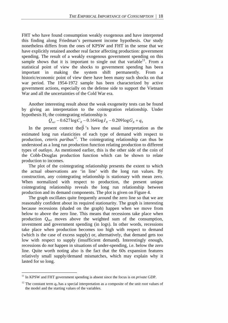
Another interesting result about the weak exogeneity tests can be found
by giving an interpretation to the cointegration relationship. Under hypothesis H2 the cointegrating relationship is
0log209.0log164.0log627.0 qGICQ RRRnet +−−−
In the present context theβ̂ ’s have the usual interpretation as the estimated long run elasticities of each type of demand with respect to production, ceteris paribus12. The cointegrating relationship can thus be understood as a long run production function relating production to different types of outlays. As mentioned earlier, this is the other side of the coin of the Cobb-Douglas production function which can be shown to relate production to incomes.
The plot of the cointegrating relationship presents the extent to which the actual observations are ‘in line’ with the long run values. By construction, any cointegrating relationship is stationary with mean zero. When normalized with respect to production, the present unique cointegrating relationship reveals the long run relationship between production and its demand components. The plot is given on Figure 4.
The graph oscillates quite frequently around the zero line so that we are reasonably confident about its required stationarity. The graph is interesting because recessions (shaded on the graph) happen when we move from below to above the zero line. This means that recessions take place when production Qnet moves above the weighted sum of the consumption, investment and government spending (in logs). In other words, recessions take place when production becomes too high with respect to demand (which is the case of excess supply) or, alternatively, that demand gets too low with respect to supply (insufficient demand). Interestingly enough, recessions do not happen in situations of under-spending, i.e. below the zero line. Quite worth noting also is the fact that the 60s expansion features relatively small supply/demand mismatches, which may explain why it lasted for so long.
11 In KPSW and FHT government spending is absent since the focus is on private GDP. 12 The constant term q0 has a special interpretation as a composite of the unit root values of
the model and the starting values of the variables.

THE EMPIRICAL IMPORTANCE OF CONSUMPTION | 19
Figure 4 – The supply-demand cointegrating relationship, 1953–1972
-.003
-.002
-.001
.000
.001
.002
.003
.004
.005
1954 1956 1958 1960 1962 1964 1966 1968 1970
1965q1 : Military spending shock
1969q1 : Oil and monetary shocks
>0 : excess supply or insufficient demand
<0 : insufficient supply or excess demand
Note : shaded areas represent official recession dates as defined by the NBER. 1965q1 is a military spending shock date identified by Ramey & Shapiro [1998] and 1969q1 an oil/monetary shock identified in Hamilton [1985] and Romer & Romer [1989].
We can now give a more meaningful interpretation to the adjustment
coefficients, economically speaking. The finding that consumption and government spending are weakly exogenous translates into the proposition that those two types of outlays, taken in growth rates, are not affected by the supply/demand mismatches (deviations to the long run equilibrium). To the opposite both production and investment bear the brunt of the adjustment
process. Note that since IrQ α<α ˆˆ , the adjustment to the long run values is
mostly made through investment.
4.3. Short run coefficients The above discussion on the estimated adjustment coefficientsiα̂ ’s was
a discussion about the weights of a stationary variable, the cointegrating relationship. In this sense it was a discussion about short run coefficients. However there are other short run coefficients in the context of VEC models, namely the lagged differences of all variables, ∑ −∆Γ iti X .
The previous test of weak exogeneity was a temporal ‘feedback causality’ test in the sense that the past (t-1) equilibrium error was a regressor of each tX∆ . Another classic temporal causality test to perform is
that of Granger predictability. The idea of Granger causality is to test for the significance of the coefficients iΓ̂ for each and every variable of the model.
If those coefficients do not turn out significant for a given variable a then

THE EMPIRICAL IMPORTANCE OF CONSUMPTION | 20
variable a is not a significant predictor and can thus be taken out of the equation. Even though intuitive, it is important to note that the Granger causality tests have a specific interpretation in the context of the VECM. Indeed those are tests based on the iΓ̂ coefficients which are only one side
of the temporal ‘causality’ coin, along with the weak exogeneity tests. Granger tests are here based on coefficients iΓ̂ which are ‘out of
equilibrium’ or ‘business cycle’ coefficients. Table 4 presents the results of Granger tests together with the weak exogeneity tests. The results are based on the H1 model but they are essentially unchanged in the other models. Table 4 – Temporal ‘causality’ tests results, 1953q1–1972q1
Explained variables
∆log Qnet, t-i ∆log Qnet
---
∆log CR 0.91
∆log IR 0.11
∆log GR 0.70
∆log CR, t-i 0.21 --- 0.04 0.80 ∆log IR, t-i 0.25 0.98 --- 0.60 ∆log GR, t-i 0.27 0.86 0.13 ---
Joint Granger 0.28 0.08 0.02 0.23
pLR( 0ˆ =αi ) 0.10 0.45 0.03 0.87
Note : Reported statistics are the probabilities of ‘not causing’.
The Granger predictability tests yield most probabilities above the 10%
level so that the system does not appear very causal. The few significant causal directions all go towards real investment growth. Investment appears being significantly ‘caused’ by the past growth rates of real consumption, and borderline so by the past growth rates of real production and real government spending. The joint Granger tests confirm this finding with probability 0.02, the lower value of the model. Therefore investment is the most endogenous variable by this measure, which is in line with the weak exogeneity measure discussed earlier. This finding is important because such a high degree of endogeneity may be the cause of the high volatility of investment we observe.
On the other hand government spending appears Granger exogenous with probabilities of 0.23 and 0.28 respectively. Since government spending is also found weakly exogenous, government spending should be labelled ‘strongly exogenous’ by Johansen’s terminology. No regressor turns out significant in the government spending equation (not even the constant) so that there would remain only
tRG ε=∆ ˆlog , or alternatively ∑ε= tRG ˆlog . In
that case the changes in government spending consists entirely of the ‘surprises’
tε̂ , i.e. non anticipated events. This result makes sense in the
1953-72 era characterized by wars and active government. Finally the last two lines of Table 4 show that consumption and
production appear to be of different nature. Consumption is endogenous during the business cycle but not over the long run, while the converse is true for production.

THE EMPIRICAL IMPORTANCE OF CONSUMPTION | 21
4.4. A CONDITIONAL MODEL
All our previous findings go in the same direction of discriminating between the two weakly exogenous variables (consumption and government spending) and the two variables (production and investment) which are not weakly exogenous. Therefore we can partition the system into (respectively) m=2 variables which exhibit levels feedbacks and p-m=2 variables which do not exhibit levels feedbacks. Because weakly exogenous variables do not contain information about the long run parameters we can altogether omit them in the modelling process and estimate a partial model, conditional on weak exogeneity (Johansen[1992]). This is done in appendix B. 4.5. Variance decomposition and impulse response functions
We so far discussed the properties of the model with respect to its estimated coefficients and their significance levels. This analysis was thus of a static nature. It has provided us with the partial effects of a variable on another without accounting for the dynamics of the model.
Variance decomposition (FEVD) and impulse response functions (IRFs) are classic tools for analyzing dynamic relationships. Both are based on the idea of shocking the system and see how it reacts. After a one-time shock, variance decomposition will decompose the variance (of the forecast error) of a variable into components attributable to each and every variable of the model, and this for any horizon after the shock. The same applies to impulse-responses with a more straightforward idea : the system is shocked and the dynamic responses of the variables are traced out.
The drawback of the decomposition of variance is that the results depend on the way the variables are ordered in the model13. The classic way to order the variables is to suppose an ordering of the variables from the most likely to act first to the least likely to act as a cause. This is essentially a causal ordering from the most exogenous variable to the most endogenous variable.
We already have identified two such orderings above when addressing Granger causality and weak exogeneity. From Table 4 above it turns out that GR is always the most exogenous variable and IR the most endogenous. The rankings of Qnet and CR are uncertain so that we simulated two shocks: shock A with ordering (GR, Qnet CR, IR) and shock B with ordering (GR, CR, Qnet, IR). We consequently decomposed the variance of the forecast error, following a shock consistent with those two orderings, and up to a 20 quarter-horizon (5 years). Because we are utmost interested in the growth process we will concentrate here upon the decomposition of production only. The results are the following:
13 Pesaran & Shin [1998] alleviates this issue in the context of impulse-response functions.
See their article for their method of ‘generalized’ impulse-responses applied on the KPSW data.

THE EMPIRICAL IMPORTANCE OF CONSUMPTION | 22
- (shock A) : at each time horizon, the variance of production is attributable almost entirely to its own shocks (>92%). As a result consumption, investment and government spending contribute for almost nothing (<8%) to the variance of production. Those results are disappointing, because we would have expected the whole (production) to depend on its components (outlays) in some non null proportion.
- (shock B) : no such problem occurs. The variance (of the forecast error) of is attributable to consumption shocks at a level comprised between 60% (when the shock occurs) and 76% (5 years after the shock). The effect of production shocks on itself accounts for most of the rest, between 33% and 19% for the same horizons. As a result investment and government spending shocks account for virtually none of the variance of production.
What should be recalled of those two decompositions of variance remains uncertain. There is no universally better way to define a ‘typical’ shock. It would however be fair to give more weight to the results pertaining to ordering B, and therefore conclude in the direction that consumption shocks explain most of the variance of production. This result is in line with KPSW who find consumption explaining ‘typically less than half of the business cycle variability (private production, in context)’ Figure 5 – IRFs of real ‘command-basis’ production, 1953q1–1972q1
-.010
-.005
.000
.005
.010
.015
.020
2 4 6 8 10 12 14 16 18 20
Response following a production shock
-.010
-.005
.000
.005
.010
.015
.020
2 4 6 8 10 12 14 16 18 20
Response following a real consumption shock
-.010
-.005
.000
.005
.010
.015
.020
2 4 6 8 10 12 14 16 18 20
Response following a real investment shock
-.010
-.005
.000
.005
.010
.015
.020
2 4 6 8 10 12 14 16 18 20
Response following a real governement spending shock

THE EMPIRICAL IMPORTANCE OF CONSUMPTION | 23
The generalized impulses-responses have also been computed up to a time horizon of 5 years. The responses have been calculated following a one-standard error shock on each impulse variable (consumption, investment and government spending). This was done on the unrestricted underlying VAR model with no further restriction14. Figure 5 presents the responses of production together with their (analytic) 95% confidence interval.
Figure 5 presents interesting patterns. Much of the dynamics have become constant at the 5-year horizon so those values can be understood as long run values. - Consumption is the only type of outlay to have a persistent effect on
production. As such an increase in consumption is likely to increase production for a long time. This finding is just the mirror image of the weak exogeneity of consumption.
- Investment has a positive impact on production but becomes not significant after 6 quarters. This means that investment shocks have a short-lived effect on production. This confirms our prior finding of investment having no persistent long run effects.
- Government spending is found to have a positive but not significant effect on production, except maybe for one quarter. This finding may appear surprising in such a period characterized by wars. However, it has to be recalled that, during the whole sample, the war effort as well as other government expenses have been entirely financed by taxes recollection. As a result the United States had a balanced budget on that period, even a slight surplus. However we previously found government spending to be strongly exogenous. This finding is not at odds with the present result, since the weak exogeneity of government spending can be understood as government spending shocks having long run effects on another variable than production.
- Production shocks are found to have positive effects on itself but, ever since 6 quarters, those effects are not clearly significant. Again, this consistent with the previous finding of production being borderline weakly exogenous.
***
Several points stand out as a conclusion of the analysis on this first
subsample 1953-1972. We find consumption as weakly exogenous based on formal tests and impulse-response functions. To the contrary investment is found very endogenous with respect to the short and the long run. Both of these findings, however, are not new, for they have already been spelled out in the studies of KPSW and FHT. Nonetheless this paper relies on more detailed tests, especially with regard to the stability of the estimated model, and also conducts the analysis in a more general framework including government spending. In this framework we have found consumption
14 The results differ little when restrictions are imposed, and the general interpretation
remain unchanged.

THE EMPIRICAL IMPORTANCE OF CONSUMPTION | 24
having an even greater role, being the cause of between 60% and 76% of the variance of production, whereas KPSW have found it to be around 40%.
The inclusion of government spending in the model leads to several interesting findings. First, including government spending reduces the number of stationary relationships, as compared to KPSW and FHT, from two to one. Second, government spending is strongly exogenous and its shocks will leave persistent effects on at least one of the variables of the model. That variable, however, is not production and this may appear surprising. 5. Estimation on the second regime
The same study was conducted after the end date of the first regime, 1972. Because the specification and identification procedure is unchanged we will not go into many details.
A VAR model was searched from 1973q1 to the end of the full sample, 2005q3. The rationale for choosing a start date of 1973 is that Chow tests results are unreliable after the first break date, precisely because the occurrence of a break changes the parameters of the model under investigation. The longest period on which the model was found stable is 1973q1-1986q1. The resulting small sample (T=53 observations) does not allow one to compute many of Chow’s statistics, so that stability analysis may prove to be hazardous.
A VEC(3) model was nonetheless found stable baring in mind those limitations. The residuals showed evidence of significant pikes on 1978q2, 1980q2, 1982q4 and 1983q4 and the subsequent dummy variables were introduced15. The VAR residual specifications are reported in Table 1 and fulfill reasonably the requirement of Gaussian errors. The cointegration tests were performed and gave rise to the same results as in preceding period, namely that there is one cointegrating relationship of either case 4 or case 3. Again, the small sample size is likely to undermine the cointegration test results, so that those results should be taken as information rather than conclusive evidence. Case 4 was rejected on the basis of the non significance of the trend in the cointegration relationship. (case 3 again)16. The results of the structural parameters are reported in Table 5.
15 The criteria retained for the introduction of a dummy variable was that there was that (1)
there was a sudden pike in the residuals and (2) that pike corresponded to a known event. The date 1978q2 corresponds to a sudden uptick in activity which had signalled the start of a formidable interest rate hikes. It is identified as a monetary shock by Romer & Romer [1989]. The most significant date 1980q2 was found in the production and consumption residuals and corresponds to several events : the ‘Carter-Reagan military build-up’ evidenced by Ramey & Shapiro [1998], an all-time high in interest rates and a policy and political change. The date 1982q4 was found in the investment residuals and corresponds to a sudden increase in the interest rates when the trend was thought to be clearly downwards. The date 1983q4 was found in the government spending equation and calls for a cut in social spending at the same time as tax breaks for businesses.
16 The constants in the VAR were estimated with t-ratios of 1.85, 4.46, -0.98 and 1.25, resulting in their joint significance. We checked for the magnitude of the largest roots of

THE EMPIRICAL IMPORTANCE OF CONSUMPTION | 25
Table 5 – Estimates of structural parameters, 1973q1–1986q1 log Qnet log CR log IR log GR ∑βiˆ
Unrestricted model
β̂ 1 -0.889 [-11.13]
-0.028 [-1.48]
-0.124 [-1.27]
0.0414
'α̂ +0.60 [-4.79]
-0.52 [-4.80]
-1.98 [-2.86]
+0.05 [0.31]
pLR( 0ˆ =αi ) 0.00 0.00 0.00 0.78
Unrestricted model 3 – H3 : 0ˆ =β∑ i (p-value 0.22)
β̂ 1 -1.009 [-14.66]
+0.001 [0.06]
+0.008 [0.15]
0
'α̂ -0.49 [-4.64]
-0.40 [-4.22]
-1.81 [-3.17]
0.09 [0.66]
pLR( 0ˆ =αi ) 0.00 0.00 0.00 0.39
Unrestricted model 4 – H3 with H 4 : 0ˆˆ =β=β GrIr and 0ˆ =αGr (p-value 0.69)
β̂ -1 1 0 0 0
'α̂ +0.52 [5.12]
+0.41 [4.27]
+1.84 [3.20]
0
Note : significant coefficients are given a bold face.
As before the model was first estimated without restrictions and then
restricted according to the results. The unrestricted model on the top panel of Table 5 indicates that the coefficient of logCR is very high and significant, that the coefficients to logIR and logGR are almost zero and not significant and that the sum of the estimated coefficients is almost zero. The model was subsequently re-estimated by imposing H3 : 1ˆˆˆ −=β+β+β GrIrCr
and the results on the middle panel indicate that this restriction was accepted with a probability of 0.22. That didn’t change much the estimates of βα,
except for that Crβ̂ is now almost unity. We therefore tested for H4 :
0ˆˆ =β=β GrIr in addition to 0ˆ =αGr . This restriction was accepted with a
high p-value of 0.69. The results appear in the bottom panel of Table 6, where normalization was done on consumption rather than on production to facilitate interpretation.
The identified structure is surprising, interesting and puzzling at the same time. In particular the elasticity of production with respect to consumption has been accepted to be one, so that the elasticities with respect to investment and government spending are zero. That finding can be understood as the fact that, on 1973-1986, besides short run movements,
the system with different number of cointegrating relationships. With one postulated cointegrating relationships the largest roots have values of 1, 1, 1, 0.77, 0.77… and with two postulated relationships they became 1, 1, 0.99, 0.77, 0.77… Clearly, the choice of a single cointegrating relationship is a better choice.

THE EMPIRICAL IMPORTANCE OF CONSUMPTION | 26
the variables ‘in line with each other’ are production and consumption only. Investment and government spending played role ‘on average’ on 1973-86.
The finding that government spending is not aligned is not a big surprise since we made a similar observation based on Figure 1 (government spending started to diverge from the other variables since the early seventies). From an economic standpoint, the early seventies denote the beginning of a ‘less government’ era. Therefore our result of government spending non-alignment makes sense and, since elasticities sum to unity, less government means higher elasticities of consumption and investment.
However, more surprising is the finding that the long run elasticity of production with respect to investment is zero as well. That means that investment has not contributed to production on average on 1973-1986. One way to make sense of this finding is to call upon the accumulation of specific events on that period: two oil shocks, stagflation, historic rise and fall of the interest rate, turn-around policy and large deficits, just to name a few. Indeed in such an uncertain world it is not surprising to see investment being hit a lot and loose track of the other variables in the process. Therefore the apparent disconnection of investment may be attributable to the (somewhat intense) accumulation of specific destabilizing events.
Finally the error-correction term deserves a comment. The long run part of the model under H4 is estimated as (in expectancy) 0loglog =− netR QC
so that the long run value of the share of consumption in net production is stationary. The plot of the cointegrating relationship is given on Figure 6 (model H4 with normalization on production for comparative purposes). Figure 6 – The supply-demand cointegrating relationship, 1973–1986
-.04
-.03
-.02
-.01
.00
.01
.02
.03
73 74 75 76 77 78 79 80 81 82 83 84 85
=0 : supply equals demand (production equals consumption)
>0 : excess supply or under-consumption
<0 : insufficient supply or excess consumption

THE EMPIRICAL IMPORTANCE OF CONSUMPTION | 27
Again the recessions (shaded) show up to be closely associated with excess supply and not with excess demand. This is particularly the case following the first oil shock and the small recession of 1980. However as compared to the previous period the association is less close. The 1981-82 recession in particular covers partly an excess supply and an excess demand stage. Contrary to the previous period 1953-1972, recessions do not end at the excess supply peak but last until excess demand is generated. Quite worth noting recessions take place when the wage share is below average.
The effects of those supply-demand mismatches can readily be seen on the adjustment coefficients. We see all variables react to it except for government spending. As during the previous period, investment reacts with the most important force so that the supply/demand mismatches are being mostly captured by investment changes. Note also that investment, not being significant in the long run, is very active in the short run.
A compared as to the 1953-1972 period, some noticeable changes have
taken place both on the long run and adjustment coefficients. The first and obvious change is that the elasticity of production with respect to consumption has risen from 0.63 to unity, while the elasticity of production with respect to government spending falls to zero, all things equal. The 1973-86 period thus marks the end of the alignment of government spending (together with investment), making production depend solely on consumption spending in the long run.
The second major change takes place in the adjustment coefficients, both in magnitude and significance levels. The magnitudes of the adjustment coefficients have been much reduced in 1973-86 as compared to 1953-72. The magnitude of the adjustment realized by production has been divided by three and that of investment has been slashed by a factor of 7+. This means that the adjustment between production (supply) and demand has taken more time during 1973-86 than it previously did. Equivalently we find a more sluggish adjustment process in the 1973-86 period, a time of less active government action.
In both periods production and investment are endogenous and government spending is exogenous17. Therefore the second most important change is to be found in the behavior of consumption, which has moved from being weakly exogenous (even borderline strongly exogenous). This process of endogeneization of consumption changes the role of consumption, from being autonomous in the first subsample to being a passive adjusting factor in the second period. Recall however that production is found to depend solely on consumption ‘on average’
Granger causality tests have also been performed on that second period.
The results are summarized in Table 6 for the model H3 and commented below.
Investment growth is, and stays, the most highly caused variable in the system, whereas consumption has now become exogenous in the short run. 17 Note that since government spending is not significant in the cointegrating relationships,
government spending cannot be deemed ‘weakly exogenous’ as in the preceding period

THE EMPIRICAL IMPORTANCE OF CONSUMPTION | 28
Production appears predicted by each and every other variable while government spending is not predicted by any other variable. As compared to the previous period those short run results have not changed by much for government spending and investment, while consumption has gained exogeneity and production has gained endogeneity. The Granger ordering has now become CR, GR, Qnet, IR. Table 6 – Temporal ‘causality’ tests results, 1973q1–1986q1
Explained variables ∆log Qnet ∆log CR ∆log IR ∆log GR
∆log Qnet, t-i --- 0.14 0.06 0.62 ∆log CR, t-i 0.09 --- 0.05 0.42 ∆log IR, t-i 0.04 0.20 --- 0.65 ∆log GR, t-i 0.11 0.55 0.18 ---
Joint Granger 0.09 0.29 0.00 0.09
pLR( 0ˆ =αi ) 0.00 0.00 0.00 0.39
Note : Reported statistics are the probabilities of ‘not causing’, derived from a Wald test.
With that new ordering the decomposition of the variance (of the
forecast error) of production didn’t change much as compared to the previous subperiod (ordering B). For any time horizon until 5 years, consumption shocks now explain between 45% and 60% of the variance of production, and the rest of it is explained by own production shocks. Consequently and as previously, investment and government spending are responsible of almost none of the variance of production. Those results are robust to alternative orderings.
The generalized impulse-responses have been computed with the same parameters as on the previous sample. The responses of production are reported on Figure 7 together with the 95% confidence intervals.
The time profiles of the production responses have changed as compared to the previous period. No variable is found to have a long lasting (permanent) effect on production. However the effect of consumption is again the most important in the short run but becomes not significant after 9 quarters. The effects of production and investment are positive in the very short run but become not significant after 2-3 quarters. Government spending is again found to have no large effect on production, if any. Note that all those results are in line with the previous finding of no weak exogeneity of production, consumption and investment. The result of government spending having no effect on production is however puzzling, for government has been very active during that period, at least during its later part. This result, which we also found during the previous period, may be an indication that production ought better be taken net of taxes.

THE EMPIRICAL IMPORTANCE OF CONSUMPTION | 29
Figure 7 – IRF of real ‘command-basis’ production, 1973q1–1986q1
-.03
-.02
-.01
.00
.01
.02
.03
2 4 6 8 10 12 14 16 18 20
Response following a real production shock
-.03
-.02
-.01
.00
.01
.02
.03
2 4 6 8 10 12 14 16 18 20
Response following a real consumption shock
-.03
-.02
-.01
.00
.01
.02
.03
2 4 6 8 10 12 14 16 18 20
Response following a real investment shock
-.03
-.02
-.01
.00
.01
.02
.03
2 4 6 8 10 12 14 16 18 20
Response following a real governement spending shock
Broadly speaking the impulse-response functions on 1973-86 do not differ much from those on 1953-72. However there seems to be some kind of shift downward of all responses, i.e. production reacts less to demand impulses. As a result all demand effects on production are found null in the long run, that is there is no permanent stimulus to production. This is essentially the characteristic of a ‘short run’ economy which is dominated by an uncertain environment characterized by important shocks on demand.
We have tried to perform the previous analysis on a more
contemporaneous period. All trials have failed because the estimates of the model were not stable for any sufficiently long sample. As a result no result will be presented here. We will however provide comments on the likely reasons why our modeling attempts have failed. 1- The most important reason seems to be that the adjustments are slow
since the eighties. This is visible in the observed lesser variance of production, as well as in shorter recessions, and consequently in longer expansions. Therefore the supply-demand mismatches are expected to oscillate less frequently around the zero line, undermining the stationarity of the error-correction term.
2- The model may be inappropriate on that period. In particular we have relied until now on a model featuring production net of trade. Yet trade has not been balanced on that period, nor has it been constant, so that it may be useful to distinguish the trade effects explicitly.

THE EMPIRICAL IMPORTANCE OF CONSUMPTION | 30
6. Estimation on the full sample
As we have seen both models have led to estimates which are not very different in nature. Besides a model estimated on the full sample period 1954-2005 had been checked to give somewhat stable estimates on the basis of Chow’s FC test. It would be interesting how the results reached so far compare to the full-sample model, even if its properties are not very satisfying.
Again we will report only the main results here. The parameters of the model are the one described above, a VAR(5) with 5 dummy variables and with residuals lacking normality. The cointegration tests were performed and unambiguously yielded r= 1 cointegrating relationship of either case 4 or case 3. Again case 4 was rejected on the basis that the trend coefficient in the cointegrating relationship turned out at most barely significant and in any case very small. The estimates of the model are presented in Table 7 for case 3.
Table 7 – Estimates of structural parameters, 1954q1–2005q3 log Qnet log CR log IR log GR ∑βiˆ
Unrestricted model
β̂ 1 -0.569 [-38.98]
-0.215 [-23.77]
-0.211 [-16.68]
0.004518
'α̂ +0.37 [-2.74]
-0.07 [-0.68]
+3.34 [5.63]
-0.32 [-1.64]
pLR( 0ˆ =αi ) 0.01 0.48 0.00 0.13
Unrestricted model 5 – H5 : 0ˆ =β∑ i (p-value 0.42)
β̂ 1 -0.556 [-38.51]
-0.219 [-22.53]
-0.224 [-42.15]
0
'α̂ +0.33 [2.83]
-0.08 [-0.82]
+3.12 [5.65]
-0.22 [-1.22]
pLR( 0ˆ =αi ) 0.01 0.51 0.00 0.32
Unrestricted model 6 – H5 with H 6 : 0ˆ,ˆ =αα CrGr (p-value 0.39)
β̂ 1 -0.557 [-37.99]
-0.219 [-22.15]
-0.224 [-41.50]
0
'α̂ +0.43 [5.12]
0 +3.20 [5.88]
0
Note : significant coefficients are given a bold face.
The model can successively be identified and restricted by imposing the sum of the demand elasticities of production to equal one (hypothesis H5, individually accepted at 0.42) jointly with the weak exogeneity of consumption and government spending (hypothesis H6, accepted at 0.39). The estimates do not change much throughout the restriction process and stay very highly significant. The cointegrating relationship of model 6 is plotted on Figure 8.

THE EMPIRICAL IMPORTANCE OF CONSUMPTION | 31
Again the model captures the recessions (shaded on the graph) very well. Almost systematically the recessions appears at the very start of excess supply and come to an end the peak of the excess supply episodes. Again, there is a time lag in between the end of the recession and the appearance of excess demand. Note the building up of excess demand following the two latest recessions 1990 and 2001 has taken more than following the previous recessions. This suggests, paradoxically, a slower adjustment than previously. Figure 8 – The supply-demand cointegrating relationship, 1954–2005
-.012
-.008
-.004
.000
.004
.008
.012
.016
.020
.024
55 60 65 70 75 80 85 90 95 00 05
=0 : supply meets demand
>0 : excess supply or insufficient demand
<0 : excess demand, insufficient supply
The results of Granger tests, performed on model 5, are reported in Table 8. Table 8 – Temporal ‘causality’ tests results, 1953q1–1972q1
Explained variables
∆log Qnet, t-i ∆log Qnet
---
∆log CR 0.00
∆log IR 0.27
∆log GR 0.63
∆log CR, t-i 0.36 --- 0.29 0.61 ∆log IR, t-i 0.99 0.01 --- 0.52 ∆log GR, t-i 0.89 0.01 0.12 ---
Joint Granger 0.00 0.03 0.00 0.62
pLR( 0ˆ =αi ) 0.01 0.51 0.00 0.32
Note : Reported statistics are the probabilities of ‘not causing’.
Those short run results are also similar to those reached on subsamples. By this measure, investment is the most endogenous variable while government

THE EMPIRICAL IMPORTANCE OF CONSUMPTION | 32
spending is the most exogenous. Since government spending has been found to be weakly exogenous, it can be deemed strongly exogenous. But this is no the case of consumption. Accounting for weak exogeneity results does not alter the Granger ordering which is here GR, CR, Qnet, IR.
Based on that ordering the decomposition of the variance (of the forecast error) of production has been performed for a period of 5 years. The results are that 51% the variance of production is explained by its own values at one quarter after the shock and falls to below 10% at 10 quarters after the shock. What captures the most of production’s variability is again consumption, in a range of 58% to 82% (respectively at a two quarters and 20 quarters after the shock). This leaves almost no room for investment (explaining below 1%) or government spending (explaining below 10% of production variability). Thus again consumption is the variable that captures the most of the business cycle variability, to a larger extent than KPSW have estimated.
The generalized responses of production are given in Figure 9. Those are essentially unchanged as compared to the results on the subsamples. Investment has a short-lived effect, consumption has a more important and persistent effect, and government spending is almost inefficient except for in the very short run. Of notable difference, though, is the persistence of production shocks on itself which turns out more significantly than on the previous subsamples. Figure 9 – IRFs of real ‘command-basis’ production, 1954q1–2005q3
-.004
.000
.004
.008
.012
.016
2 4 6 8 10 12 14 16 18 20
Response following a real production shock
-.004
.000
.004
.008
.012
.016
2 4 6 8 10 12 14 16 18 20
Response following a real consumption shock
-.004
.000
.004
.008
.012
.016
2 4 6 8 10 12 14 16 18 20
Response following a real investment shock
-.004
.000
.004
.008
.012
.016
2 4 6 8 10 12 14 16 18 20
Response following a real governement spending shock

THE EMPIRICAL IMPORTANCE OF CONSUMPTION | 33
TENTATIVE CONCLUSION
The issue dealt with in this article is that of the role of the variables in a
model featuring production, consumption, investment and government spending. To that extent we have modeled those variables expressed in real terms within an error-correction model framework. We have distinguished between the results pertaining to the full-sample 1954-2005 and two subperiods, 1953-72 and 1973-86 on which the model was found more stable. No stable model could be found on a period starting after 1986. The results can be classified in two groups : the new or surprising ones, and the ones consistent with the previous empirical literature (KPSW and FHT, albeit using a different model).
There are several results consistent with the previous literature. The first and most important is that consumption shocks, above all other types of demand, has the largest and more persistent effect on production. Investment on the other hand is found to have a short-lived, temporary effect on production. Those two findings are already present in KPSW and FHT. Therefore our results provide robustness to their original findings when other samples, parameters, and variables are used.
Our new findings come precisely from such a different methodology. First we have inquired about the stability of the models, which KPSW and FHT do not do. Stability is indeed required for the reason that breaks are likely to greatly affect the estimates of the model, and that breaks are highly likely to have happened in a 50+ year long sample. Splitting the sample did not reverse the previous findings, and to the contrary has reinforced the importance of consumption. For instance we find consumption shocks to account for at least 45% and 60% of the variance of production on our two subsamples, significantly more than previously estimated by KPSW.
Another original feature of the present paper has been to feature government spending explicitly in the model. As commented above this did not change the previous findings about the relative importance of consumption and investment for production. However two main results have arisen from the introduction of government spending in the model.
The first one is that there now exists only one cointegrating relationship (clearly), as compared to two in KPSW and FHT. Their study consisted of three variables out of which only one was found weakly exogenous (consumption). With two cointegrating relationships, the authors have identified all the permanent component of the model as (proportional to) the cumulated sum of the unexpected consumption shocks. Therefore the models of KPSW and FHT do not leave any room for investment as part of the permanent component. Clearly this is at odds with most economic theories –provided that consumption shocks are not interpreted as productivity or permanent income shocks. Most theories, indeed, call upon investment to be one, if not the only, factor of growth. Yet in both KPSW and FHT models, investment has no role of giving a general tendency to the system.
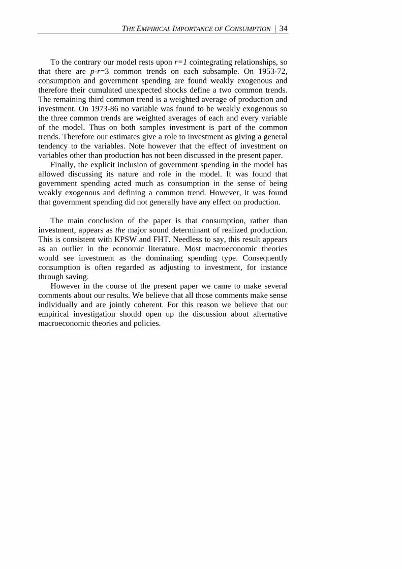
THE EMPIRICAL IMPORTANCE OF CONSUMPTION | 34
To the contrary our model rests upon r=1 cointegrating relationships, so that there are p-r=3 common trends on each subsample. On 1953-72, consumption and government spending are found weakly exogenous and therefore their cumulated unexpected shocks define a two common trends. The remaining third common trend is a weighted average of production and investment. On 1973-86 no variable was found to be weakly exogenous so the three common trends are weighted averages of each and every variable of the model. Thus on both samples investment is part of the common trends. Therefore our estimates give a role to investment as giving a general tendency to the variables. Note however that the effect of investment on variables other than production has not been discussed in the present paper.
Finally, the explicit inclusion of government spending in the model has allowed discussing its nature and role in the model. It was found that government spending acted much as consumption in the sense of being weakly exogenous and defining a common trend. However, it was found that government spending did not generally have any effect on production.
The main conclusion of the paper is that consumption, rather than
investment, appears as the major sound determinant of realized production. This is consistent with KPSW and FHT. Needless to say, this result appears as an outlier in the economic literature. Most macroeconomic theories would see investment as the dominating spending type. Consequently consumption is often regarded as adjusting to investment, for instance through saving.
However in the course of the present paper we came to make several comments about our results. We believe that all those comments make sense individually and are jointly coherent. For this reason we believe that our empirical investigation should open up the discussion about alternative macroeconomic theories and policies.

THE EMPIRICAL IMPORTANCE OF CONSUMPTION | 35
REFERENCES
Bureau of Economic Analysis, National Income and Products Accounts, http://www.bea.gov/
Candelon B., Lütkepohl H. [2001] On the Reliability of Chow-type Tests for Parameter Constancy in Multivariate Dynamic Models, Economics Letters, 73, 155–160
Cheung Y., Lai K [1993] Finite-Sample Sizes of Johansen's Likelihood Ration Tests for Cointegration, Oxford Bulletin of Economics and Statistics, 55, 3, 313-28
Cochrane J. [1994] Permanent and Transitory Components of GNP and Stock Prices, Quarterly Journal of Economics, 109, 241–265
Dickey D., Fuller W. [1981] The Likelihood Ratio Statistics for Autoregressive Time Series with a Unit Root, Econometrica, 49, 4, 1047-1072
Elliott G., Rothenberg T., Stock J. [1996] Efficient Tests for an Autoregressive Unit Root, Econometrica, 64, 813-836
Engle R., Granger C. [1987] Co-integration and Error Correction: Representation, Estimation, and Testing, Econometrica, 55, 251-276
Fama E. [1992] Transitory Variation in Investment and Output, Journal of Monetary Economics, 30, 467–480
Fisher L., Huh H., Tallman E. [2003] Permanent Income and Transitory Variation in Investment and Output, Journal of Macroeconomics, 25, 149–168
Godfrey L. [1988] Misspecification Tests in Econometrics, Cambridge University Press, Cambridge
Hamilton J. [1985] Historical Causes of Postwar Oil Shocks and Recessions, Energy Journal, 6, 97-116
Hansen H. Johansen S. [1999] Some Tests for Parameter Constancy in the Cointegrated VAR, Econometric Journal, 2, 306-333
Jarque C., Bera, A. [1987] A Test for Normality of Observations and Regression Residuals, International Statistical Review, 55, 163-172
Johansen S. [1988] Statistical Analysis of Cointegration Vectors, Journal of Economic Dynamics and Control, 12, 2-3, 231-254
Johansen S. [1991] Estimation and Hypothesis Testing of Cointegration Vectors in Gaussian Vector Autoregressive Models, Econometrica, 59, 1551-1580
Johansen S. [1992] Testing Weak Exogeneity and the Order of Cointegration in UK Money Demand, Journal of Policy Modeling, 14, 313–334
Johansen S. [1995] Likelihood-Based Inference in Cointegrated Vector Autoregressive Models, Advanced Texts in Econometrics, Oxford University Press, Oxford, UK
Johansen S. [1995] Likelihood-Based Inference in Cointegrated Vector Autoregressive Models, Oxford University Press, Oxford, New York
Johansen & Juselius [1990] Maximum Likelihood Estimation and Inference on Cointegration – with Applications to the Demand for Money, Oxford Bulletin of Economics and Statistics, 52, 169-210
Johansen S., Juselius K. [1992] Structural Tests in a Multivariate Cointegration Analysis of the PPP and UIP for UK, Journal of Econometrics, 53, pp. 211-244
King R., Plosser C., Stock J., Watson M. [1991] Stochastic Trends and Economic Fluctuations, American Economic Review, 81, 819–840

THE EMPIRICAL IMPORTANCE OF CONSUMPTION | 36
Kwiatkowski D., Phillips P., Schmidt P., Shin Y. [1992] Testing the Null Hypothesis of Stationary against the Alternative of a Unit Root, Journal of Econometrics, 54, 159-178
Lütkepohl H., Kräzig M. [2004] Applied Time Series Econometrics, Cambridge University Press, Cambridge
Newbold P., Leybourne S., Wohar M. [2001] Trend-Stationarity, Difference-Stationarity, or Neither: Further Diagnostic Tests with an Application to U.S. Real GNP, Journal of Economics and Business, 53,1, 85-102
Pesaran M., Shin Y. [1998] Impulse Response Analysis in Linear Multivariate Models, Economics Letters, 58, 17-29
Ramey V., Shapiro M. [1998] Costly Capital Reallocation and the Effects of government Spending, Carnegie-Rochester Conference Series on Public Policy, 48, 145-194
Reimers H. [1992] Comparisons of Tests for Multivariate Cointegration, Statistical Papers, 33, 335-359
Romer C., Romer D. [1989] Does Monetary Policy Matter : A New Test in the Spirit of Friedman and Schwartz, in : Blanchard O., Fisher F. NBER Macroeconomics Annual, 63-129
Saikkonen P., Lütkepohl H. [2000a] Testing for the Cointegrating Rank of a VAR Process with an Intercept, Econometric Theory, 16, 373-406
Saikkonen P., Lütkepohl H. [2000b] Testing for the Cointegrating Rank of a VAR Process with Structural Shifts, Journal of Business & Economic Statistics, 18, 451-464
Saikkonen P., Lütkepohl H. [2000c] Trend Adjustment Prior to Testing for the Cointegrating Rank of a Vector Autoregressive Process, Journal of Time Series Analysis, 21, 435-456
Shaikh A. [1974] Laws of Production and Laws of Algebra : The Humbug Production Function, Review of Economics and Statistics, 56, 115-120

THE EMPIRICAL IMPORTANCE OF CONSUMPTION | 37
– APPENDIX A – – An intuitive interpretation of VEC models –
The VEC models can quickly become very complicated and it is useful to have an intuitive interpretation of their most interesting feature : their rich structure. We will here take the simple example of a VEC model with no dummies and no lagged values, i.e. k=1 and a constant. In that case
ttt uXX +µ+Π= −11
where we take only two variables for simplicity, namely Xt={ yt, ct} consists GDP and consumption (in logs). This is a VAR model which states that (1) production at t-1 affects present consumption jointly with (2) consumption at t-1 affects present production. Alternatively, this VAR model can be rewritten in its error-correction form as
( ) ttt XX ε+γ+β−βα=∆ − 001'
For illustrative purposes we will set the values of the long run parameters to [ ]11' −=β so that the cointegrating relationship is
0111 loglog:' β−+−β −−− ttt cyX
Note that the long run β parameters are generally estimated by Johansen’s method rather than chosen as we do here.
By construction the cointegrating relationship is always stationary so that ( ) 0' 1 =β −tXE . This implies that the cointegrating relationship can be
rewritten as 0))/(log( β=ycE , i.e. 0β is the average value of (the log of) the
share of consumption in GDP. By our choice of parameters the model above gives the changes in GDP and consumption as explained by the share of consumption in GDP, and a constant 0γ .
In applied work production and consumption have often been found to exhibit the same pattern through time, i.e. to be cointegrated. As a result a scatter plot of the two variables will show points disseminated around an average relationship which takes the form of an upward-trending line. The choices made above give this line the equation 0loglog β+= YC , i.e. a 45°
line originating in 0β . This is the cointegrating relationship, i.e. the steady-
state relationship which holds ‘on average’ or ‘in the long run’. This line is plotted in Figure A below.

THE EMPIRICAL IMPORTANCE OF CONSUMPTION | 38
Figure A – An intuitive representation of a VECM
note: derived from Juselius[2006], chap. 5, p.102.
The graph consists of the following different parts. )( ⊥βSp is the
space spanned by the long run parameters, i.e. the straight, upward-trending line evidenced above. However this relationship is true ‘in the long run’ only and the observations (yt, ct) are almost never on that line. The most likely case is that deviations appear in the short run such as point xt. Here xt is figured such as it is above the cointegrating relationship, that is consumption and production are such as the share of consumption is above its long run value. Whenever a deviation appears the error-correction mechanism is activated so that a force α moves both variables. The direction and magnitude of the error-correction mechanism depends on the long run parameters as well asα . For the chosen long run values, the deviation xt is likely to be corrected for by a negative force α affecting GDP and/or consumption changes.
In applied work the long run parameters are estimated to be very close to [ ]11' −=β . The estimates of the adjustment coefficients would turn out
as )0,( yα=α with yα <0. Equivalently, production adjusts and
consumption is weakly exogenous. This means that consumption is found not to depend on the consumption share while production does, or alternatively that the log run stability of the consumption share in GDP is maintained by adjustments of GDP only. Consequently the unanticipated shocks to consumption define the common trend ∑εcˆ while GDP assures
the stability of the system. This general result translates into the proposition that shocks to consumption would persist in time, while shocks to GDP would merely be transitory.
consumption (x1t = log ct)
0β

THE EMPIRICAL IMPORTANCE OF CONSUMPTION | 39
– APPENDIX B – – The partial model 1953-1972 –
The idea of a partial model in the context of VECMs is the following.
Take { }endo
t
exog
tt XXX ,= as the vector of p variables of interest which is
split into m weakly exogenous variables exogtX and p-m variables endo
tX which are not weakly exogenous. In that case the full VEC model, say
of the form
t
k
i
ititt uXXX +µ+∆Γ+αβ=∆ ∑−
=−− 0
1
1
1'
yields the same estimated set of β̂ coefficients than the partial model
t
exog
t
k
i
it
endo
it
endoendo
t vXAXXX +∆+η+∆Γ+βα=∆ ∑−
=−− 00
1
1
1'
The partial model therefore is the same as the full model (where only the equations for the non weakly exogenous variables remain) augmented by
exog
tX∆ as an additional regressor. Note that this regressor is specified as an
exogenous variable, i.e. only the values at time t remain. Why estimate partial models instead of full models ? The question is not
as naïve as it seems because estimating a partial model requires to know which variables are weakly exogenous, that is most of the time requires to estimate the full model in the first place. The answer to this question is that by conditioning on weakly variables one reduces the number of parameters as well as the number of equations to estimate. Consequently in practice a partial model is often found more stable and precise than a full model. However, using a partial model to describe a process in the short run is clearly not a good modelling strategy since the weak exogeneity holds with respect to the long run parameters. Partial models ought therefore be only used when the long run properties of a system are the focus.
We have estimated the partial model conditional on the weak exogeneity of both consumption and government spending. For comparative purposes we first report the equations of production and investment of the full model under H2.
=σ=+−++
++++−−βα=
=σ=++++
++++−−βα=
−−
•
−
•
−
•
−
•
−
•
−
•
−
•
−−
•
−−
•
−
•
−
•
−
•
−
•
−
•
−
•
−
•
−−
•
−−
•
046.0,133.0ˆ020.064.294.1
75.184.131.896.938.1114.12'ˆˆ
010.0,136.0ˆ002.050.025.0
33.027.042.135.102.246.1'ˆˆ
2
,]61.1[
2,]81.1[
1,]19.1[
2,]73.1[
1,]61.1[
2,]87.1[
1,]12.2[
2,]66.1[
1,]61.1[
1,
2
,]89.0[
2,]55.1[
1,]69.0[
2,]46.1[
1,]09.1[
2,]44.1[
1,]30.1[
2,]33.1[
1,]87.0[
1,
RuGG
IICCQQXI
RuGG
IICCQQXQ
tIrtRtR
tRtRtRtRtnettnett
FFtR
tQnettRtR
tRtRtRtRtnettnett
FF
tnet
where for compacity we use the •
=∆ tt AA :log shorthand notation, and where

THE EMPIRICAL IMPORTANCE OF CONSUMPTION | 40
FF βα ˆ,ˆ are the adjustment and long run parameters for the full model we already discussed and which are given in the bottom panel of Table 5.
The partial model had PP βα ˆ,ˆ parameters such as
915.0log*209.0log*164.0log*627.0log]00.103[]86.70[]85.169[
−−−−−−−
RRRnet GICQ
and the adjustment coefficients became ]91.1[54.1ˆ +=αP
Q and ]54.2[64.13ˆ −=αP
Ir
which is unchanged as compared to the FF βα ˆ,ˆ estimates for the full model up to the third decimal. The detailed partial model was estimated as
=σ=+
−+−++
++++−−βα=
=σ=+
++−++
++++−−βα=
•
−
•
−−
•
−
•
−
•
−
•
−
•
−
•
−
•
−−
•
−−
•
••
−
•
−
•
−
•
−
•
−
•
−
•
−
•
−−
•
−−−
•
040.0,358.0ˆ40.043.3044.010.335.2
96.180.181.829.1076.1225.13'ˆˆ
006.0,707.0ˆ15.013.1006.051.039.0
32.030.045.167.113.219.2'ˆˆ
2
,,]21.1[
,]96.4[]67.3[
2,]46.2[
1,]67.1[
2,]24.2[
1,]83.1[
2,]30.2[
1,]54.2[
2,]16.2[
1,]04.2[
1,
2
,,]09.3[
,]93.10[]43.3[
2,]70.2[
1,]87.1[
2,]44.2[
1,]02.2[
2,]51.2[
1,]74.2[
2,]40.2[
1,]24.2[
1,
RvGCGG
IICCQQXI
RvGCGG
IICCQQXQ
tIrtRtRtRtR
tRtRtRtRtnettnett
PPtR
tQnettRtRtRtR
tRtRtRtRtnettnett
PP
tnet
As compared to the short run part of the full model, the estimates of the partial model have changed especially in terms of significance levels.
In the full model no coefficient in the production equation was found significant at the 10% level. In the partial model all eleven coefficients become significant at the 5% level, five are significant at 1% and two at are significant at the 1‰ level. The adjusted R² increased dramatically from 14% to 70% of the variance of the growth rate of production being explained by the model. The standard error of the equation was almost slashed by two to 0.6%.
The same applies to the investment equation. In the full model there are eight coefficients (out of eleven) which are significant at the 10% level and one at the 5% level. In the partial model ten coefficients are significant at the 10% level, eight at 5%, three at the 1% level and two at the 1‰ level. The fit increased also by much, moving from 13% to 36%. The standard error of the equation, however, didn’t drop by much.
Other statistics worth commenting are the coefficients of the variables acting as exogenous regressors (reported into brackets). Those are ‘short run’ or ‘spot’ coefficients as weights of stationary variables. They can be understood as elasticities calculated with acceleration rates. All coefficients are highly significant except for the contemporaneous effect of government spending on investment (however, past values of government spending foster investment). The largest contemporaneous effect if that of consumption on investment (+3.43) and the lowest is that of government spending on production (+0.15). The ‘spot’ value of consumption on production is 1.13, meaning that an acceleration of consumption by
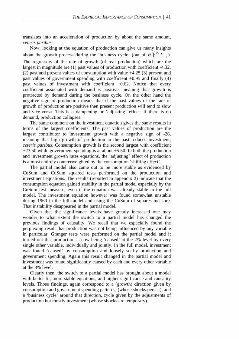
THE EMPIRICAL IMPORTANCE OF CONSUMPTION | 41
translates into an acceleration of production by about the same amount, ceteris paribus.
Now, looking at the equation of production can give us many insights about the growth process during the ‘business cycle’ (out of 1'ˆˆ −βα t
PP X ).
The regressors of the rate of growth (of real production) which are the largest in magnitude are (1) past values of production with coefficient -4.32, (2) past and present values of consumption with value +4.25 (3) present and past values of government spending with coefficient +0.95 and finally (4) past values of investment with coefficient +0.62. Notice that every coefficient associated with demand is positive, meaning that growth is protracted by demand during the business cycle. On the other hand the negative sign of production means that if the past values of the rate of growth of production are positive then present production will tend to slow and vice-versa. This is a dampening or ‘adjusting’ effect. If there is no demand, production collapses.
The same comment on the investment equation gives the same results in terms of the largest coefficients. The past values of production are the largest contributor to investment growth with a negative sign of -26, meaning that high growth of production in the past reduces investment, ceteris paribus. Consumption growth is the second largest with coefficient +23.50 while government spending is at about +5.50. In both the production and investment growth rates equations, the ‘adjusting’ effect of production is almost entirely counterweighted by the consumption ‘shifting effect’.
The partial model also came out to be more stable as evidenced by CuSum and CuSum squared tests performed on the production and investment equations. The results (reported in appendix 2) indicate that the consumption equation gained stability in the partial model especially by the CuSum test measure, even if the equation was already stable in the full model. The investment equation however was found somewhat unstable during 1960 in the full model and using the CuSum of squares measure. That instability disappeared in the partial model.
Given that the significance levels have greatly increased one may wonder to what extent the switch to a partial model has changed the previous findings of causality. We recall that we especially found the perplexing result that production was not being influenced by any variable in particular. Granger tests were performed on the partial model and it turned out that production is now being ‘caused’ at the 2% level by every single other variable, individually and jointly. In the full model, investment was found ‘caused’ by consumption and loosely so by production and government spending. Again this result changed in the partial model and investment was found significantly caused by each and every other variable at the 3% level.
Clearly then, the switch to a partial model has brought about a model with better fit, more stable equations, and higher significance and causality levels. Those findings, again correspond to a (growth) direction given by consumption and government spending patterns, (whose shocks persist), and a ‘business cycle’ around that direction, cycle given by the adjustments of production but mostly investment (whose shocks are temporary).