I. Introduction

For many years, the conditions of lifein the poorest of poor neighborhoodshave attracted the attention of film-makers, journalists, and academic

researchers. Each in their own way, these witnesses provide stark evidence about the

devastating effects impoverished environ-ments can have on those unfortunate enoughto dwell within them, and about how theseeffects spill over into society at large.

Poverty, in government statistics, is definedon the basis of a family’s income relative to afixed poverty line, a standard meant to reflectthe cost of basic necessities. This narrow,

May 2003 • The Brookings Institution The Living Cities Census Series 1

“This report docu-

ments a dramatic

decline in the

1990s in the

number of

high-poverty

neighborhoods,

their population,

and the concen-

tration of the

poor in these

neighborhoods.”

Center on Urban and Metropolitan Policy

■ The number of people living in high-poverty neighborhoods—where thepoverty rate is 40 percent orhigher—declined by a dramatic 24percent, or 2.5 million people, inthe 1990s. This improvement markeda significant turnaround from the1970–1990 period, during which thepopulation in high-poverty neighbor-hoods doubled.

■ The steepest declines in high-poverty neighborhoods occurred inmetropolitan areas in the Midwestand South. In Detroit, for instance,the number of people living in high-poverty neighborhoods dropped nearly75 percent over the decade.

■ Concentrated poverty—the share ofthe poor living in high-povertyneighborhoods—declined among allracial and ethnic groups, especiallyAfrican Americans. The share of poor

black individuals living in high-povertyneighborhoods declined from 30 per-cent in 1990 to 19 percent in 2000.

■ The number of high-poverty neigh-borhoods declined in rural areas andcentral cities, but suburbs experi-enced almost no change. A number ofolder, inner-ring suburbs around majormetropolitan areas actually experiencedincreases in poverty over the decade,though poverty rates there generallyremain well below 40 percent.

While the 1990s brought a landmarkreversal of decades of increasingly con-centrated poverty, the recent economicdownturn and the weakening state ofmany older suburbs underscore that thetrend may reverse once again withoutcontinued efforts to promote economicand residential opportunity for low-income families.

FindingsA national analysis of high-poverty neighborhoods, and the concentration of poor individu-als in those neighborhoods, in 1990 and 2000 indicates that:

Stunning Progress, Hidden Problems:The Dramatic Decline of Concentrated Poverty in the 1990sPaul A. Jargowsky1

bookkeeper’s conception of poverty,however, fails to capture the multipleways in which poverty acts to degradethe quality of life and limit the oppor-tunities of those in its grip. One of themost important aspects of poverty notcaptured in the official statistics is itsspatial dimension. In theory, poor fam-ilies and their children could be widelydispersed throughout the population.In fact, they often tend to live nearother poor people in neighborhoodswith high poverty rates. The problemis particularly acute for the minoritypoor, who are segregated by both raceand income.

Why should we be concerned withthe spatial organization of poverty?The concentration of poor familiesand children in high-poverty ghettos,barrios, and slums magnifies the problems faced by the poor. Concen-trations of poor people lead to a con-centration of the social ills that causeor are caused by poverty. Poor childrenin these neighborhoods not only lackbasic necessities in their own homes,but also they must contend with a hos-tile environment that holds manytemptations and few positive role mod-els. Equally important, school districtsand attendance zones are generallyorganized geographically, so that theresidential concentration of the poorfrequently results in low-performingschools. The concentration of povertyin central cities also may exacerbatethe flight of middle-income andhigher-income families to the suburbs,driving a wedge between social needsand the fiscal base required to addressthem.

Between 1970 and 1990, the spatialconcentration of the poor rose dramat-ically in many U.S. metropolitanareas.2 The number of people living inhigh-poverty areas doubled; thechance that a poor black child residedin a high-poverty neighborhoodincreased from roughly one-in-four toone-in-three; and the physical size ofthe blighted sections of many centralcities increased even more dramati-

cally. By contrast, poverty—measuredat the family level—did not increaseduring this period. Thus, there was anot a change in poverty per se, but afundamental change in the spatialorganization of poverty. The poorbecame more physically isolated fromthe social and economic mainstreamof society.

Two key factors contributed to theincreasing concentration of povertyduring the 1970s and 1980s. First,weaknesses in local or regionaleconomies tended to disproportion-ately impact central cities. And sec-ondly, exclusionary suburbandevelopment patterns contributed toincreasing economic segregation.

Policymakers have been anxious toknow how the spatial organization ofpoverty may have changed in the1990s. For most metropolitan areasand the country as a whole, thedecade was a period of unparalleledeconomic growth. However, rapid sub-urban development continued andperhaps even accelerated during thisperiod. The net effect of these trendson the concentration of poverty in the1990s is therefore ambiguous.

Only the decennial Census providessufficient detail at the neighborhoodlevel to examine the concentration ofpoverty. With the release of Census2000, we are now able to assess thenet impact of the economy, suburbandevelopment, and other forces on thespatial dimension of poverty over thelast decade.

Based on the trend of prior decades,one might have reasonably assumedthat high-poverty neighborhoods werean unavoidable aspect of urban lifeand would continue to grow inexorablyin size and population. The latest evi-dence contradicts this gloomy assess-ment. This report documents adramatic decline in the 1990s in thenumber of high-poverty neighbor-hoods, their population, and the con-centration of the poor in theseneighborhoods. It also finds, however,several indications that poverty rose in

the older suburbs of many metropoli-tan areas, even during a decade of eco-nomic expansion. The paper concludeswith a discussion of the meaning ofthese trends, and the more recentdecline in economic conditions, forpoor families and communities in thecurrent decade.

II. Methodology

This report examines thechanges in the concentrationof poverty in the 1990s usingsample data (the “long form”)

from the 1990 and 2000 decennialcensuses.

For the purpose of this study,poverty is defined using official U.S.poverty guidelines. An individual isconsidered poor if he lives in a familywhose income is less than a specificthreshold that varies by family size andcomposition. While the official defini-tion suffers from a number of knownflaws and limitations, it is neverthelesswidely accepted.3 More importantly,the Census Bureau provides data onpoverty status based on the long formof the census.

In everyday usage, one can talkabout a neighborhood in general termswithout specifying exact boundaries.For tabulation purposes, however,every household in the nation mustreside in one and only one geographi-cally specific neighborhood. In thisstudy, we use census tracts as proxiesfor neighborhoods. Census tracts aresmall, relatively homogeneous areasdevised by the Census Bureau andlocal planning agencies, making use of bounding features such as majorroads, railroad tracks, and rivers when-ever possible. On average, they con-tain 4,000 persons, but in practicethey vary widely in population. Theyalso vary widely in geographic size dueto differences in population density.When initially delineated, censustracts are meant to be relatively homo-geneous with respect to social andeconomic characteristics and housing

May 2003 • The Brookings Institution The Living Cities Census Series2

stock considerations. While they maynot always capture the mental map ofneighborhoods that city residentshave, they do divide the nation alonggeographic lines. In less dense ruralareas, one census tract may representall or a substantial portion of a county.

As populations grow and change,census tracts may be split, merged, ormodified in other ways. In thisresearch, contemporaneous tracts areused. That is, 1990 census tractboundaries are used to interpret 1990data, and 2000 census tract bound-aries are used for the 2000 figures.Using contemporaneous boundaries isimportant, because to do otherwisewould invite a systematic bias into theanalysis. For example, if the 2000 cen-sus tract grid were superimposed on1970 data, average neighborhood pop-ulation would be far smaller in 1970than in 2000. Defining neighborhoodsdifferently over time would systemati-cally bias the results of any analysisthat is sensitive to the size of theneighborhood units.4

Combining the poverty dimensionand the spatial dimension, a censustract is considered a high-povertyneighborhood if 40 percent or more ofits residents are classified as poorusing the federal poverty standard.While any specific threshold is inher-ently arbitrary, the 40 percent level hasbecome the standard in the literature

and has even been incorporated intofederal data analysis and programrules.5 In addition to tabulating thenumber of high-poverty neighborhoodsand the number and characteristics oftheir residents, this paper examinesthe concentration of poverty—definedas the percentage of the poor in somecity or region that resides in high-poverty neighborhoods.

These two concepts—the incidenceof high-poverty neighborhoods, andthe concentration of poverty—are notunrelated. In general, the greater thenumber of high-poverty neighborhoodsin a city or metropolitan area is, themore likely poor residents of that placewill be “concentrated” in those neigh-borhoods. However, each measureanswers a different question. The for-mer relates to the geographic footprintof very-low-income districts within acity or metropolitan area, which hasimportant implications for economicdevelopment efforts and city planning.The latter captures the percentage ofpoor individuals who not only mustcope with their own low incomes, butalso with the economic and socialeffects of the poverty that surroundsthem.

The figures presented below includeall census tracts in the United States,including both metropolitan and non-metropolitan areas, except as noted. Ametropolitan area usually consists of

one or more population centers, orcentral cities, and the nearby countiesthat have close economic and com-muting ties to the central cities.6 TheCensus Bureau defines several typesof metropolitan areas. There arestand-alone Metropolitan StatisticalAreas (MSAs) and Primary Metropoli-tan Statistical Areas (PMSAs). PMSAsare part of larger constructions calledConsolidated Metropolitan StatisticalAreas (CMSAs). In this analysis, met-ropolitan areas are defined to includeMSAs and PMSAs, not CMSAs.CMSAs are so large that they do notrepresent unified housing and labormarkets, and so they are not consid-ered in this analysis.7

Like census tracts, the boundariesof metropolitan areas are adjusted overtime. New counties are added, andexisting counties are deleted or movedto different metropolitan areas if thereare changes in their demographics, inthe commuting patterns of their resi-dents, or if the Census Bureauchanges the rules for allocating coun-ties to metropolitan areas. In thisanalysis, the definitions of metropoli-tan areas (including MSAs andPMSAs) in effect for Census 2000 areapplied to both 1990 and 2000 data.In keeping with this, any changes inthe figures for metropolitan areasshown below reflect actual changes inpopulation demographics and notchanges in boundaries or definitions.

To examine variation among racialand ethnic groups, population isdivided first by Hispanic origin, andthen non-Hispanics are further dividedby racial group—black, white, Ameri-can Indian, Asian, and people whoindicated more than one race (in2000) or “other race.” Thus, a refer-ence to whites refers to non-Hispanicpersons who indicated “White or Cau-casian” as their sole racial group onthe census form, a reference to blacksindicates non-Hispanic persons whochose “Black or African-American” astheir sole race, and so on.

A final methodological note: A por-

May 2003 • The Brookings Institution The Living Cities Census Series 3

The Federal Poverty Standard

Developed by Molly Orshansky of the Social Security Administration in the1960s for use in the War on Poverty, the federal poverty standard has beencriticized from every conceivable angle. Despite its imperfections, it hasendured as both an administrative tool to determine program eligibility andas a research tool. Persons are considered poor if they live in families whosetotal family income is less than a threshold meant to represent the cost ofbasic necessities. The thresholds vary by family size, and are adjusted eachyear for inflation. For example, in 2002, the poverty level was $15,260 for atypical family of three and $18,400 for a typical family of four. For moreinformation, see Orshansky (1965), Fisher (1992), and the HHS poverty website: aspe.hhs.gov/poverty/poverty.shtml.

tion of this study analyzes levels andchanges in high-poverty neighbor-hoods based on their location in cen-tral cities, suburbs, or rural areas. Inpractice, census tracts are subdivisionsof counties, and thus often do notrespect the municipal borders thatdefine central cities.8 In such cases,the tract’s poverty status is classifiedby the poverty rate for the entire tract.That is, there is only one poverty ratefor each whole census tract, no matterhow many ways the tract is split overcity or metropolitan boundaries. Inthis way, the count of persons residingin high-poverty areas is consistent, andsystematic biases that would arisefrom the splitting of census tracts areavoided.

III. Findings

A. The number of people living inhigh-poverty neighborhoods—wherethe poverty rate is 40 percent orhigher—declined by a dramatic 24percent, or 2.5 million people, inthe 1990s.The strong economic conditions thatprevailed throughout most of the1990s appear to have dramaticallyaltered long-term trends in the spatialorganization of poverty. The number ofhigh-poverty neighborhoods—censustracts with poverty rates of 40 percentor more—declined by more than one-fourth, from 3,417 in 1990 to 2,510 in2000 nationwide. This is a stunningreversal of the trend between 1970and 1990, as shown in Figure 1.9

More importantly, the total numberof residents of high-poverty areasdeclined by 24 percent, from 10.4 mil-lion in 1990 to 7.9 million in 2000.The sharp decline does not merelyreflect declines in overall poverty. Infact, despite the strong economy, thenumber of persons classified as poorin the United States actually rosebetween 1990 and 2000, from 31.7million to 33.9 million. The overallpoverty rate did decline over thedecade (from 13.1 percent to 12.4 per-

cent), but by a much smaller degreethan did the number of high-povertyneighborhoods. The implication is thatthere was a substantial change in thespatial organization of poverty duringthe 1990s. Poor neighborhoods, or atleast the residents of high-povertyneighborhoods in 1990, benefited dis-proportionately from the boom.

Virtually the whole spectrum ofracial and ethnic groups benefitedfrom the decline in the number of per-sons residing in high-poverty neighbor-hoods. The number of white residentsof these areas declined by 29 percent(from 2.7 to 1.9 million), and thenumber of black residents declined byan even faster 36 percent (from 4.8million to 3.1 million). Despite thisdecline, however, blacks remained thesingle largest racial/ethnic group livingin high-poverty neighborhoods.

The major exception to the patternwas Hispanics, whose numbers inhigh-poverty neighborhoods actuallyincreased slightly, by 1.6 percent. Atthe same time, the number of Hispan-ics in the U.S. overall increased dra-matically in the 1990s—by 57.9

percent, compared to only 3.4 percentgrowth for whites and 16.2 percent forblacks. In the context of this rapidpopulation growth, fueled by theimmigration of many low-income per-sons from Central and South America,as well as births to immigrant families,a growth rate of only 1.6 percent inthe number of Hispanics in high-poverty neighborhoods could beviewed as a positive outcome.

Given that different racial and eth-nic groups were growing at differentrates, the composition of high-povertyzones changed over the period. Figure2 shows how the population in high-poverty neighborhoods changedbetween 1990 and 2000 by race andethnicity. Hispanic and Asian sharesincreased, while those for whites andblacks declined. Most notably, Hispan-ics now comprise a larger share ofhigh-poverty neighborhood residentsthan whites.

B. The steepest declines in high-poverty neighborhoods occurred inmetropolitan areas in the Midwestand South.

May 2003 • The Brookings Institution The Living Cities Census Series4

3,500

3,000

2,500

2,000

1,500

1,000

500

0

9,000

8,000

7,000

6,000

5,000

4,000

3,000

2,000

1,000

0

Hig

h Po

vert

y N

eigh

borh

oods

High Poverty N

eighborhood Population (1000s)

1970 1980 1990 2000

■ High-Poverty Neighborhoods High-Poverty Neighborhood Population (thousands)

Figure 1. High-Poverty Neighborhoods and High-PovertyNeighborhood Population, U.S. Metropolitan Areas, 1970–2000

Based on metropolitan areas as defined in year of census.

Earlier research indicated that theexpansion of high-poverty ghettos andbarrios was particularly acute in theMidwest, especially in central cityneighborhoods. Now, the Midwest hasexhibited the most rapid turnaroundduring the boom of the 1990s.

As shown in Figure 3, populationchanges in high-poverty areas varieddramatically across regions of thecountry. In general, places with thelargest declines in the number of high-poverty neighborhoods also expe-rienced the steepest drops in the num-ber of people living in such areas.10

The decline was largest in the Mid-west, where the population of high-poverty neighborhoods was nearlyhalved over the decade. There was alsoa substantial decline in the South,which nonetheless remained home tothe largest number of high-povertyneighborhoods in 2000.

At the same time, the number ofhigh-poverty neighborhoods in theNortheast remained virtually the samein 2000 as in 1990, and the Westactually saw a substantial 26 percentincrease in the population of these

neighborhoods, albeit from a smallbase. In 1990, the population of high-poverty neighborhoods in the Westwas half that in the Midwest; by 2000,nearly 300,000 more people lived in

high-poverty neighborhoods in theWest than in the Midwest. Thisincrease is explained almost entirely byan increase in the size and populationof Hispanic barrios; the number of

May 2003 • The Brookings Institution The Living Cities Census Series 5

0

500

1,000

1,500

2,000

2,500

3,000

3,500

4,000

4,500

5,000

West(+25.9%)

South(-34.7%)

Midwest(-45.6%)

Northeast(-0.3%)

■ 1990■ 2000

1,839 1,823

2,526

1,374

4,712

3,077

1,3281,672

Figure 3. Population of High-Poverty Neighborhoods by Region,1990–2000

Black 47%

White 26%

Asian 2%

Hispanic 22%

Other 3%

Black 39%

Hispanic 29%

Asian 4%

White 24%

Other 4%

1990 2000

Figure 2. Racial/Ethnic Composition of High-Poverty U.S. Neighborhoods, 1990–2000

Popu

lati

on (

thou

sand

s)

non-Hispanic persons in high-povertyareas in the West declined slightly.

While only two out of four regionsshowed significant declines in theaggregate, the view at the state level ismore positive. Figure 4 maps the per-centage change in high-poverty neigh-borhood population by state. Fully 40states had declines, with an averagedecline of 78,000 persons residing inhigh-poverty neighborhoods. Tenstates, as well as the District ofColumbia, had increases averaging61,000 persons. Trends in the West asa whole are clearly driven by Califor-nia, which had an 87 percent increasein the population of high-povertyneighborhoods.

Table 1 shows the 15 metro areaswith the largest decreases in high-poverty-area population. The regionalflavor is readily apparent. Withoutexception, the metropolitan areaslisted are located in the Midwest or inthe South. Detroit’s decline in thepopulation of high-poverty neighbor-hoods was substantially larger than inany other metropolitan area. Chicago,however, experienced a comparabledecrease in the number of high-poverty census tracts. All told, 200 outof 331 metropolitan areas (MSAs andPMSAs) saw declines in the numberof people living in high-poverty neigh-borhoods (Appendix A shows relevantdata for all U.S. metropolitan areas,and non-metropolitan areas by state).

In most metropolitan areas, high-poverty neighborhoods tend to be clus-tered in one or two mainagglomerations located in the centralcity. In this way, the United States dif-fers markedly from most other nationsof the world, in which poor neighbor-hoods are typically located on theperiphery of urban areas. As thesezones of concentrated povertyincreased in size between 1970 and1990, they contributed to a generalprocess of population deconcentrationthat generated “donut cities”—depop-ulating and impoverished urban coressurrounded by prosperous and growing

suburbs. But then came the 1990s anda boon for central cities. Just as cen-tral cities bore the brunt of the fiscal,social, and economic burden of con-centrating poverty in prior decades,they became prime beneficiaries of its

reduction in the 1990s.A case in point is the Detroit, MI

metro area. Figure 5 shows the high-poverty zones in Detroit over threedecades. From 1970 to 1990, there isa rapid growth in the number of neigh-

May 2003 • The Brookings Institution The Living Cities Census Series6

Table 1. Top 15 Metropolitan Areas by Decline in Population ofHigh-Poverty Neighborhoods, 1990–2000

Decline in % Decline in Decline in Metropolitan Area Population Population Census TractsDetroit, MI 313,217 74.4 97Chicago, IL 177,908 43.1 73San Antonio, TX 107,272 70.1 18Houston, TX 77,662 47.8 27Milwaukee-Waukesha, WI 63,357 45.0 16Memphis, TN-AR-MS 61,924 43.6 11New Orleans, LA 57,332 34.6 18Brownsville-Harlingen-San Benito, TX 50,559 37.1 4Columbus, OH 48,020 55.4 11El Paso, TX 44,489 40.2 4Dallas, TX 41,805 45.3 19St. Louis, MO-IL 38,866 35.5 13Lafayette, LA 33,978 54.8 10Minneapolis-St. Paul, MN-WI 32,005 40.5 18Flint, MI 31,631 61.2 6

Figure 4. Percentage Change in Population of High-PovertyNeighborhoods by State, 1990–2000

Change, 1990–2000

May 2003 • The Brookings Institution The Living Cities Census Series 7

Figure 5. High-Poverty Neighborhoods in Detroit, 1970–2000

1970

1990

1980

2000

Figure 6. High-Poverty Neighborhoods in Dallas, 1970–2000

1970

1990

1980

2000

borhoods with poverty rates of 40 per-cent or more. By 1990, nearly half theland area of the City of Detroit, theboundary of which is shown in yellow,had become a high-poverty zone. Thistrend is reversed between 1990 and2000. The change is so dramatic, itstrains credulity. To some extent, thevivid map colors may overstate thechange, since many of Detroit’s censustracts had all but emptied out by1990. Thus, a movement or change inpoverty status of just a few familiescould serve to change the color of anentire census tract on the map. Evenso, the Detroit metro area underwentan astonishing 74.4 percent reductionin the number of people residing inhigh-poverty zones between 1990 and 2000.

The growth of high-poverty zonesbetween 1970 and 1990 and their sub-sequent declines were by no meanslimited to the Midwest. Figure 6shows the trend in the Dallas metro-

politan area over the last threedecades. The poverty areas of Dallasexperienced their greatest expansionbetween 1980 and 1990, after the col-lapse of the OPEC oil cartel led tosharply lower oil prices. At the sametime, Dallas was also experiencingrapid suburban development. Plano,TX, a “Boomburb” just north of Dallas,was for years the fastest growing cityin the nation.12 After 1990, however,there was substantial redevelopment

of the downtown area, including con-dominium and apartment develop-ments just north of downtown andalong Interstate 45. The overalldecline in the population of Dallas’shigh-poverty areas was 45 percentbetween 1990 and 2000.

The regional picture is quite differ-ent when we examine the metropolitanareas with the largest increases inhigh-poverty area population. Seven ofthe 15 metropolitan areas in Table 2

May 2003 • The Brookings Institution The Living Cities Census Series8

Mapping Poor Neighborhoods

The maps shown in these figures were produced using an interactive website.By visiting the web site, users can easily produce maps such as these for anymetropolitan area in the United States. The address for the web site iswww.urbanpoverty.net. Construction of the web site was funded by theBrookings Institution Center on Urban and Metropolitan Policy and the Bru-ton Center for Development Studies at the University of Texas at Dallas.Comments and suggestions about the web site are welcome.11

Figure 7. High-Poverty Neighborhoods in Los Angeles, 1970–2000

1970

1990

1980

2000

are located in one state—California—and six of those lie in either southernCalifornia or the state’s agriculturalhub, the San Joaquin Valley. Othermetro areas include a handful in theNortheast (Providence, Wilmington,Rochester, and two suburban New Jer-sey metros) and two smaller metros inTexas. Altogether, a total of 91 out of331 metropolitan areas had at least anominal increase in persons living inhigh-poverty neighborhoods.

It is worth noting that the size ofthe population increase in high-poverty zones falls off rapidly as weread down the list. The fifteenth met-ropolitan area, Monmouth-Ocean, NJ,had a 9,000-person increase in itshigh-poverty neighborhood population,whereas the fifteenth metropolitanarea in Table 1 (Flint, MI) had a32,000-person decline in its poverty-area population.

Figure 7 illustrates the process in LosAngeles. The expansion of high-povertyneighborhoods, indicated in red, is quiteapparent. Also apparent is a consider-able increase in the number of neigh-

borhoods with moderate poverty rates(between 20 and 40 percent).

Los Angeles is notable for three fac-tors that may explain its divergencefrom the national trend. First, the cityexperienced a deadly and destructiveriot after the Rodney King verdict in1992, and further heightening ofracial tension due to the trial of O.J.Simpson in 1995. The riot and itsaftermath almost certainly acceleratedmiddle-class flight from the centralcity area, and the trial emphasizedracial divisions in the region. Second,the Los Angeles region experiencedtremendous immigration from Mexicoand other Central and South Americancountries.13 Riverside/San Bernadino,Fresno, and (to a lesser extent) SanDiego also experienced a significantincrease in low-income Hispanic pop-ulation; the population of high-povertyneighborhoods increased in theseareas as well. Third, the recession ofthe early 1990s was particularly severein Southern California, and the eco-nomic recovery there was not as rapidas in other parts of California (such as

the San Francisco/Silicon Valley area)that benefited from the Internet boom.

The other major exception to thetrend was the Washington, D.C. metroarea. The number of high-povertyneighborhoods in the nation’s capitalmore than doubled over the decade.The major factor at work here waslikely the devastating fiscal crisis thatplagued the District during the earlyand mid-1990s. The crisis underminedpublic confidence in the governance ofthe District and led to serious cut-backs in public services, includingpublic safety. For this and other rea-sons, there was a rapid out-migrationof moderate- and middle-income blackfamilies, particularly into suburbanMaryland counties to the east of thecentral city. The poor were left behindin economically isolated neighbor-hoods with increasing poverty rates.The late 1990s real estate boom inWashington seems not to haveimproved conditions in these neigh-borhoods.

Of course, these metros and othersin Table 2 represent the exceptions toan overall decline in the number ofhigh-poverty neighborhoods, and pop-ulation of high-poverty neighborhoods,in the 1990s. Most areas of the U.S.saw improvements over the decadethat were much greater in magnitudethan the deterioration that occurred ina minority of metro areas.

C. Concentrated poverty—the shareof the poor living in high-povertyneighborhoods—declined among allracial and ethnic groups, especiallyAfrican Americans.In the 1990s, consonant with thedecline in high-poverty neighbor-hoods, the concentration of poverty—defined as the proportion of the poor ina given area that resides in high-poverty zones—dropped across most ofthe nation. The number of poor per-sons living in high-poverty areasdeclined 27 percent, from 4.8 millionto 3.5 million. In 1990, the share ofpoor individuals nationwide who lived

May 2003 • The Brookings Institution The Living Cities Census Series 9

Table 2. Top 15 Metropolitan Areas by Increase in Population ofHigh-Poverty Neighborhoods, 1990–2000

Increase in % Increase Increase in Metropolitan Area Population in Population Census TractsLos Angeles-Long Beach, CA 292,359 109.2 81Fresno, CA 60,005 68.7 12Riverside-San Bernardino, CA 58,669 260.5 12Washington, DC-MD-VA-WV 56,954 276.4 14Bakersfield, CA 42,622 190.8 9San Diego, CA 33,274 86.1 10McAllen-Edinburg-Mission, TX 28,117 12.0 (1)Providence-Fall River-Warwick, RI-MA 22,186 235.4 3Chico-Paradise, CA 16,675 103.3 4Middlesex-Somerset-Hunterdon, NJ 14,020 n/a* 3Wilmington-Newark, DE-MD 12,349 276.3 2Bryan-College Station, TX 11,746 29.4 4Visalia-Tulare-Porterville, CA 11,176 60.1 2Rochester, NY 9,989 29.8 0Monmouth-Ocean, NJ 9,114 318.3 (1)*Middlesex-Somerset-Hunterdon, NJ, had no census tracts with poverty rates of 40 percent or higher

in 1990.

in high-poverty areas (the concentratedpoverty rate) was 15 percent. By 2000,that figure had declined to 10 percent.

These declines are both striking andgratifying. Between 1970 and 1990,the concentration of poverty grewsteadily worse, especially for blacks.About one-fourth of the black poorlived in high-poverty areas in 1970; by1990, the proportion had increased toone-third. The rate was even higherfor black children, especially those insingle-parent families. The economicand social isolation of these familiesand children prompted great concernamong researchers investigating theopportunities and constraints facinglow-income families in economicallyimpoverished neighborhoods.14

Some have argued that poor personsmay benefit from having poor neigh-bors. For example, they may share coping strategies and draw on geo-graphically-based support networks.Yet most researchers, and most of thegeneral public, assume that the bene-fits of poor persons living in high-poverty neighborhoods are outweighedby the extra hardships that such neigh-borhoods impose, including their dele-terious effects on child developmentand the ability of poor adults toachieve self-sufficiency.

For those reasons, it is good newsindeed that all racial and ethnicgroups shared in the deconcentrationof poverty of the 1990s, as shown inFigure 8. The decline was most signifi-cant for poor blacks; the percentageliving in high-poverty neighborhoodsdeclined from 30.4 percent in 1990 to18.6 percent in 2000. American Indi-ans experienced a similarly largedecrease. Yet despite these substantialdeclines, blacks and American Indiansstill suffer the highest concentratedpoverty rates, the former in highly seg-regated urban ghettos and the latter inremote rural reservations. The concen-tration of poverty among non-Hispanicwhites, low to start with, dropped byroughly one-sixth. The chances that apoor Hispanic lives in a high-poverty

neighborhood dropped from morethan one in five (21.2 percent) in1990 to less than one in seven (13.8percent) in 2000.15

The declines in concentratedpoverty were not driven by a few largeor unrepresentative metropolitanareas. Indeed, substantial declineswere the national norm. Of the 331metropolitan areas in the UnitedStates in 2000, 227 (69 percent) sawthe concentration of poor blacksdecrease between 1990 and 2000;another 49 (15 percent) had nochange; and only 55 (17 percent) hadincreases (Appendix A). The story wassimilar for non-metropolitan areas:The concentration of poor blacks inrural areas declined in 29 of 49 states,and remained the same in another 11states.16

The numbers were similar, if notquite as positive, for Hispanics. Morethan half of all metropolitan areas haddecreases in concentrated Hispanicpoverty, 87 (26 percent) had increases,and the remainder experienced nochange.

The deconcentration of poverty for

racial and ethnic minorities spreadwidely across the nation’s largest met-ropolitan areas. Table 3 reports con-centrated poverty rates among blacksand Hispanics in the 20 largest met-ros, sorted by change in the concen-trated black poverty rate between1990 and 2000. Most of these areasexperienced declines in the concentra-tion of poverty for both groups. Thelargest declines for blacks were inDetroit (37.5 percentage points), Min-neapolis-St. Paul (20.3) and Chicago(18.8). Four metropolitan areas haddouble-digit percentage point declinesin the concentrated poverty rate forHispanics: Detroit (29.1 percentagepoints), Minneapolis-St. Paul (12.3),Philadelphia (12.1), and Houston(10.3).

To be sure, the percentage-pointdeclines were generally largest in areasthat had high rates of concentratedpoverty to begin with; while the shareof blacks living in high-poverty neigh-borhoods in the Seattle metro areawas halved in the 1990s, this repre-sented a decline of only 3.3 percent-age points. Still, the extent of the

May 2003 • The Brookings Institution The Living Cities Census Series10

-15

-10

-5

0

5

10

15

20

25

30

35

AsianAmericanIndian

HispanicBlackWhite

■ 1990 ■ 2000 ■ Percentage Point Change

Perc

enta

ge o

f Po

or in

Hig

h-Po

vert

y N

eigh

borh

oods

7.1 5.9

-1.2

30.4

18.6

-11.8

21.5

13.8

-7.4-11.2

-2.9

9.8

12.7

19.5

30.6

Figure 8. Concentration of U.S. Poor by Race/Ethnicity,1990–2000

decline in places like Detroit and Min-neapolis-St. Paul is remarkable com-pared to an area like New York, whichdespite modest declines still has veryhigh concentrated poverty rates forboth groups.

Consistent with the data on the pop-ulation of high-poverty areas, two areasof the country cut against the nationaltrend. In Los Angeles-Long Beach andRiverside-San Bernardino, concen-trated poverty increased among boththe black and Hispanic poor; in SanDiego, Hispanic concentrated povertyrose. In Washington, D.C., poor blacksbecame more spatially concentrated,but poor Hispanics did not.

One additional note on Westernhigh-poverty neighborhoods: In thatregion, the increase in high-povertyneighborhoods owed almost entirely to

an increase in the number of barrios—predominantly Hispanic high-povertycommunities. While increasing con-centrated poverty among Hispanics insouthern California is certainly causefor concern, researchers haveexpended considerably greater effortstudying the deleterious effects thathigh-poverty neighborhoods in theMidwest and Northeast have on thelife chances of their residents, who arepredominantly black. With their sub-stantial immigrant populations, West-ern inner-city barrios could representmore of a “gateway” to residential andeconomic mobility than inner-cityghettos in other areas of the country.Regardless, the rise in concentratedHispanic poverty in California duringthe 1990s highlights a need to betterunderstand how the opportunity struc-

ture in these communities may differfrom that in other types of high-poverty neighborhoods. 17

D. The number of high-povertyneighborhoods declined in ruralareas and central cities, but suburbsexperienced almost no change.So far, this paper has considered sta-tistics on changes in high-povertyneighborhoods and the concentrationof poverty at the national and metro-politan levels. These statistics obscurean important aspect of the trend in the1990s that the maps help illuminate:Central cities, rather than suburbs,reaped the benefits of the decline. Noteven the maps, however, reveal whattranspired in rural America. This sec-tion examines changes within metro-politan areas, and outside them, in

May 2003 • The Brookings Institution The Living Cities Census Series 1 1

Table 3. Concentration of Black and Hispanic Poverty in the 20 Largest Metro Areas, 1990–2000

Black HispanicMetro Area 1990 2000 Change 1990 2000 ChangeDetroit, MI 53.9 16.4 -37.5 36.1 6.9 -26.1Minneapolis-St. Paul, MN-WI 33.3 13.0 -20.4 18.2 5.9 -12.3Chicago, IL 45.3 26.4 -18.8 12.4 4.7 -7.7St. Louis, MO-IL 39.1 23.8 -15.3 12.8 5.2 -7.6Baltimore, MD 34.7 21.5 -13.2 9.7 3.5 -6.2Dallas, TX 25.4 13.8 -11.6 12.8 3.5 -9.3Tampa-St. Petersburg-Clearwater, FL 29.1 17.8 -11.4 7.3 4.7 -2.6Houston, TX 28.0 17.1 -10.9 13.1 2.8 -10.3Phoenix-Mesa, AZ 25.7 15.4 -10.3 21.3 12.2 -9.1New York, NY 40.1 32.5 -7.6 40.9 32.2 -8.7Philadelphia, PA-NJ 31.0 23.6 -7.5 61.6 49.5 -12.1Boston, MA-NH 12.5 6.2 -6.3 10.7 8.1 -2.6Atlanta, GA 26.6 20.5 -6.1 6.8 2.5 -4.2Seattle-Bellevue-Everett, WA 6.8 3.4 -3.3 8.1 1.3 -6.8San Diego, CA 15.4 13.0 -2.4 10.2 12.5 2.3Nassau-Suffolk, NY 0.5 0.0 -0.5 0.0 0.0 0.0Orange County, CA 0.0 0.0 0.0 0.0 0.1 0.1Los Angeles-Long Beach, CA 17.3 21.3 4.1 9.1 16.9 7.8Riverside-San Bernardino, CA 5.7 12.3 6.6 4.4 8.9 4.5Washington, DC-MD-VA-WV 6.3 15.0 8.7 1.0 0.4 -0.6

Figures represent percentage of metro-wide poor individuals in each racial/ethnic group living in census tracts with poverty rates of 40 percent or higher.

Increases shown in bold.

neighborhood poverty over the decade. All neighborhoods—census tracts—

nationwide can be classified as lyingwithin the central cities of metropoli-tan areas, the suburbs—defined as thebalance of metropolitan areas—ornon-metropolitan areas, which consistof rural areas and cities and towns toosmall or detached to be consideredpart of a metropolitan area. As shownin Figure 9, the decline in high-poverty area population was actuallylargest in non-metropolitan areas,where the decline was nearly 50 per-cent. Central city areas, as indicatedby the maps, also experienced a largedecline of 21 percent.

It was the suburbs that had theslowest overall decline in poverty arearesidents—only 4.4 percent. As aresult of these differing declines, by2000 suburban America was actuallyhome to more neighborhoods of con-centrated poverty than rural America.While the suburbs have more thantwice the number of residents as non-metropolitan areas, this finding isnonetheless striking given that theoverall poverty rate outside metropoli-tan areas (14.6 percent) was consider-ably higher in 2000 than the povertyrate in suburbs (8.4 percent).

Moreover, a careful inspection oftrends in the geography of suburbanpoverty over the 1990s reveals somedisturbing trends. Not only did thenumber of neighborhoods of highpoverty decline slowly in the suburbs.Also, poverty rates actually increasedalong the outer edges of central citiesand in the inner-ring suburbs of manymetropolitan areas, including those thatsaw dramatic declines in poverty con-centration. In short, poverty trends inthese areas moved in the oppositedirection from those in inner-cityneighborhoods and booming suburbs atthe metropolitan fringe.

Several metropolitan areas illustratethe case. Figure 10 shows the changein the poverty rate by census tractbetween 1990 and 2000 for four—Detroit, Chicago, Cleveland, and Dal-

las. Neighborhoods shaded in greenhad decreases in their poverty rates,while red indicates census tracts withincreases in their poverty rates. InDetroit, central city tracts experienceddramatic decreases in their povertyrates in the 1990s, dropping many ofthem below the 40-percent threshold.However, a ring of neighborhoods justbeyond the border of the central city—located in the area’s older suburbs—saw increases in their poverty rates.Many of these neighborhoods stillhave poverty rates of below 20 per-cent, and so cannot be consideredhigh-poverty. Yet it is notable that in adecade of widespread economicgrowth, the poverty rates in theseolder suburban neighborhoods wererising. The maps of Chicago, Cleve-land, and Dallas also exhibit the dis-tinctive “bull’s-eye” pattern ofimprovements in the central city andincreasing poverty in the inner ring ofsuburbs. This pattern is repeated inmetro areas across the nation.

The economic decline of inner-ringsuburbs, already evident in earlier

decades, continued in the 1990s evenas conditions were improving dramati-cally in most central cities.18 The factthat inner-ring suburbs declined dur-ing this period is really quite astonish-ing. Census 2000 was conducted inApril of 2000, coinciding with thepeak of a long economic boom. Unem-ployment rates nationwide were 4 per-cent, and lower in some of thesemetropolitan areas. The economy, inall likelihood, will never be strongerthan it was during this period, at leastnot for any extended period of time.

A vigorous debate is underway con-cerning the role of suburban develop-ment in central city and oldersuburban decline and the concentra-tion of poverty. There is, as yet, noconsensus that rapid suburban devel-opment, characterized as “sprawl” byits opponents, exacerbates economicdecline in the core. In fact, someargue the contrary, and contend thatthese development patterns are a con-sequence of the economic and socialdisorder of the inner cities. Thesequestions will continue to engender

May 2003 • The Brookings Institution The Living Cities Census Series12

0 1,000 2,000 3,000 4,000 5,000 6,000 7,000 8,000 9,000 10,000 11,000

Non-Metropolitan

(-47%)

Suburbs(-4%)

Central City(-21%)

Total U.S (-24%)

■ 1990■ 2000

10,394

7,946

7,560

5,988

1,089

1,041

1,745

917

Population (thousands)

Figure 9. Population of High-Poverty Neighborhoods byLocation, 1990–2000

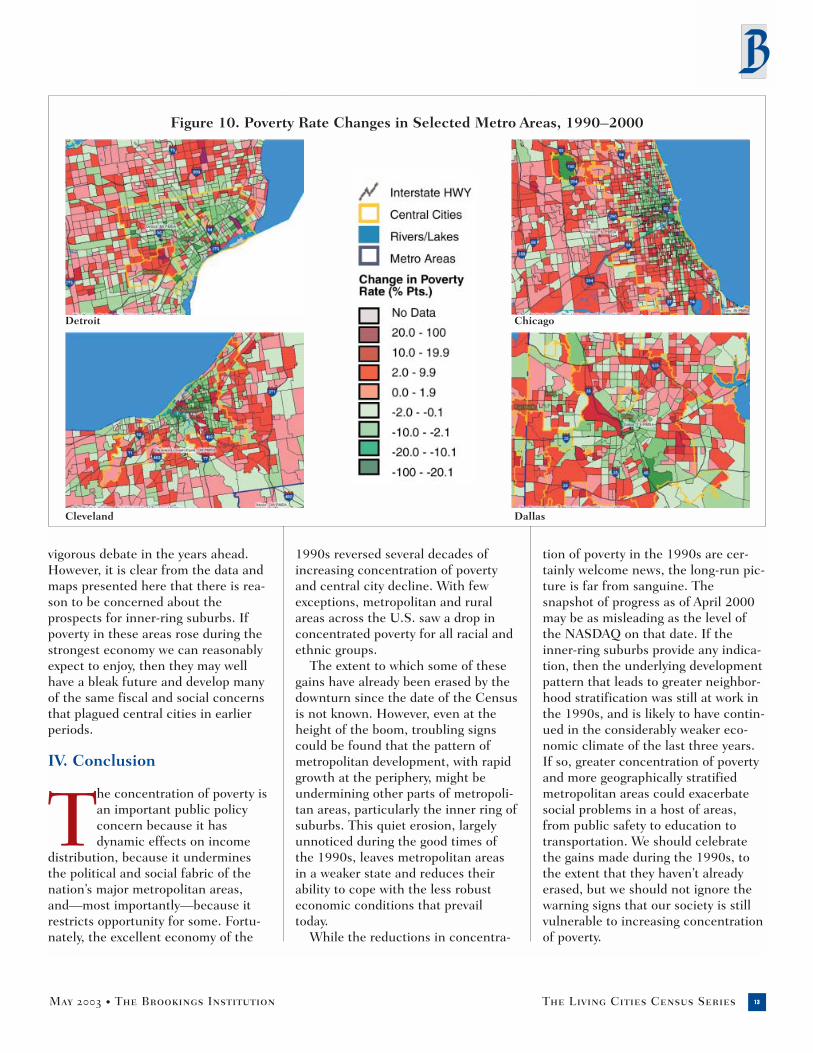
vigorous debate in the years ahead.However, it is clear from the data andmaps presented here that there is rea-son to be concerned about theprospects for inner-ring suburbs. Ifpoverty in these areas rose during thestrongest economy we can reasonablyexpect to enjoy, then they may wellhave a bleak future and develop manyof the same fiscal and social concernsthat plagued central cities in earlierperiods.

IV. Conclusion

The concentration of poverty isan important public policyconcern because it hasdynamic effects on income

distribution, because it underminesthe political and social fabric of thenation’s major metropolitan areas,and—most importantly—because itrestricts opportunity for some. Fortu-nately, the excellent economy of the

1990s reversed several decades ofincreasing concentration of povertyand central city decline. With fewexceptions, metropolitan and ruralareas across the U.S. saw a drop inconcentrated poverty for all racial andethnic groups.

The extent to which some of thesegains have already been erased by thedownturn since the date of the Censusis not known. However, even at theheight of the boom, troubling signscould be found that the pattern ofmetropolitan development, with rapidgrowth at the periphery, might beundermining other parts of metropoli-tan areas, particularly the inner ring ofsuburbs. This quiet erosion, largelyunnoticed during the good times ofthe 1990s, leaves metropolitan areasin a weaker state and reduces theirability to cope with the less robusteconomic conditions that prevailtoday.

While the reductions in concentra-

tion of poverty in the 1990s are cer-tainly welcome news, the long-run pic-ture is far from sanguine. Thesnapshot of progress as of April 2000may be as misleading as the level ofthe NASDAQ on that date. If theinner-ring suburbs provide any indica-tion, then the underlying developmentpattern that leads to greater neighbor-hood stratification was still at work inthe 1990s, and is likely to have contin-ued in the considerably weaker eco-nomic climate of the last three years.If so, greater concentration of povertyand more geographically stratifiedmetropolitan areas could exacerbatesocial problems in a host of areas,from public safety to education totransportation. We should celebratethe gains made during the 1990s, tothe extent that they haven’t alreadyerased, but we should not ignore thewarning signs that our society is stillvulnerable to increasing concentrationof poverty.

May 2003 • The Brookings Institution The Living Cities Census Series 13

Figure 10. Poverty Rate Changes in Selected Metro Areas, 1990–2000

Detroit

Cleveland

Chicago

Dallas

May 2003 • The Brookings Institution The Living Cities Census Series14

App

endi

x A

. Pop

ulat

ion

and

Num

ber

of N

eigh

borh

oods

of

Hig

h P

over

ty, a

nd C

once

ntra

ted

Pov

erty

Rat

es,

U.S

. Met

ropo

lita

n an

d N

on-M

etro

poli

tan

Are

as, 1

990–

2000

Tota

l Are

aHi

gh-P

over

ty

Popu

latio

n in

Co

ncen

trat

ed

Conc

entr

ated

Co

ncen

trat

ed

Popu

latio

nCe

nsus

Trac

tsHi

gh-P

over

ty C

ensu

s Tr

acts

Pove

rty

Rate

: Tot

alPo

vert

y Ra

te: B

lack

sPo

vert

y Ra

te: H

ispa

nics

MSA

/PM

SA/B

alan

ce o

f Sta

te N

ame

2000

1990

2000

Chan

ge19

9020

00Ch

ange

1990

2000

Chan

ge19

9020

00Ch

ange

1990

2000

Chan

geA

bile

ne, T

X12

6,55

52

1-1

1,53

658

1-9

554.

22.

2-2

.08.

04.

3-3

.77.

31.

2-6

.0A

kron

, OH

694,

960

197

-12

48,6

3222

,268

-26,

364

23.4

10.1

-13.

329

.814

.8-1

5.1

32.1

14.4

-17.

7A

lban

y, G

A12

0,82

29

7-2

23,7

2518

,700

-5,0

2549

.934

.5-1

5.4

57.9

42.2

-15.

756

.322

.7-3

3.6

Alb

any-

Sch

enec

tady

-Tro

y, N

Y87

5,58

32

64

8,65

413

,033

4,37

94.

97.

02.

124

.217

.0-7

.24.

913

.38.

5A

lbuq

uerq

ue, N

M71

2,73

85

3-2

12,5

2310

,999

-1,5

247.

15.

3-1

.81.

76.

44.

75.

54.

3-1

.2A

lexa

ndri

a, L

A12

6,33

76

5-1

15,2

0411

,854

-3,3

5026

.222

.6-3

.643

.535

.4-8

.113

.19.

2-3

.9A

llent

own-

Bet

hleh

em-E

asto

n, P

A63

7,95

82

53

9,64

114

,645

5,00

48.

110

.22.

19.

312

.12.

819

.521

.21.

7A

ltoo

na, P

A12

9,14

41

10

1,70

21,

739

373.

84.

30.

512

.816

.33.

40.

00.

00.

0A

mar

illo,

TX

217,

858

72

-58,

093

3,16

8-4

,925

12.7

4.3

-8.5

27.7

13.4

-14.

317

.33.

9-1

3.4

Anc

hora

ge, A

K26

0,28

30

00

00

00.

00.

00.

00.

00.

00.

00.

00.

00.

0A

nn A

rbor

, MI

578,

736

88

036

,182

28,9

37-7

,245

24.4

25.2

0.8

10.0

25.8

15.8

11.1

14.8

3.7

Ann

isto

n, A

L11

2,24

93

2-1

6,49

85,

076

-1,4

2217

.910

.5-7

.440

.118

.4-2

1.7

62.8

3.7

-59.

1A

pple

ton-

Osh

kosh

-Nee

nah,

WI

358,

365

21

-17,

348

5,61

4-1

,734

7.6

5.3

-2.3

8.9

3.8

-5.1

6.6

0.5

-6.1

Ash

evill

e, N

C22

5,96

53

2-1

3,12

74,

507

1,38

05.

67.

21.

614

.633

.919

.20.

08.

68.

6A

then

s, G

A15

3,44

47

81

23,6

5131

,425

7,77

433

.240

.57.

354

.542

.1-1

2.5

17.4

13.8

-3.7

Atl

anta

, GA

4,11

2,19

836

31-5

92,0

5392

,039

-14

15.3

11.1

-4.2

26.6

20.5

-6.1

6.8

2.5

-4.2

Atl

anti

c-C

ape

May

, NJ

354,

878

44

09,

282

9,90

762

513

.79.

4-4

.333

.326

.8-6

.514

.58.

0-6

.5A

ubur

n-O

pelik

a, A

L11

5,09

27

6-1

22,3

5723

,876

1,51

950

.644

.4-6

.239

.237

.3-2

.034

.250

.616

.4A

ugus

ta-A

iken

, GA

-SC

477,

441

77

022

,132

18,2

46-3

,886

17.6

12.3

-5.3

25.2

18.8

-6.4

12.6

6.5

-6.0

Aus

tin-

San

Mar

cos,

TX

1,24

9,76

312

7-5

45,4

2345

,057

-366

14.4

12.3

-2.1

17.9

11.0

-6.9

15.5

8.1

-7.4

Bak

ersf

ield

, CA

661,

645

413

922

,333

64,9

5542

,622

11.5

22.0

10.5

29.7

36.3

6.6

15.1

28.5

13.4

Bal

tim

ore,

MD

2,55

2,99

438

33-5

106,

648

75,6

43-3

1,00

522

.513

.5-9

.034

.721

.5-1

3.2

9.7

3.5

-6.2

Ban

gor,

ME

90,8

641

10

1,13

24,

241

3,10

93.

05.

32.

30.

07.

07.

014

.60.

0-1

4.6

Bar

nsta

ble-

Yarm

outh

, MA

162,

582

00

00

00

0.0

0.0

0.0

0.0

0.0

0.0

0.0

0.0

0.0

Bat

on R

ouge

, LA

602,

894

169

-760

,375

42,4

01-1

7,97

428

.317

.6-1

0.7

34.8

17.5

-17.

334

.229

.7-4

.5B

eaum

ont-

Port

Art

hur,

TX

385,

090

154

-11

23,3

117,

858

-15,

453

17.9

6.1

-11.

833

.011

.7-2

1.3

12.2

1.4

-10.

8B

ellin

gham

, WA

166,

814

11

05,

941

6,91

897

79.

88.

2-1

.59.

56.

3-3

.31.

01.

91.

0B

ento

n H

arbo

r, M

I16

2,45

37

4-3

15,7

169,

690

-6,0

2637

.323

.5-1

3.8

75.0

50.4

-24.

65.

30.

0-5

.3B

erge

n-Pa

ssai

c, N

J1,

373,

167

35

25,

483

11,7

556,

272

3.0

4.9

1.9

12.2

18.1

5.9

1.1

3.6

2.5

Bill

ings

, MT

129,

352

21

-14,

088

3,59

2-4

9612

.19.

9-2

.256

.58.

5-4

8.0

27.0

31.5

4.5

Bilo

xi-G

ulfp

ort-

Pasc

agou

la, M

S36

3,98

84

2-2

9,30

588

1-8

,424

8.4

0.1

-8.3

12.3

0.0

-12.

30.

00.

00.

0B

ingh

amto

n, N

Y25

2,32

02

31

4,36

65,

446

1,08

07.

07.

30.

317

.613

.4-4

.25.

612

.77.

0B

irm

ingh

am, A

L92

1,10

614

10-4

54,8

7133

,631

-21,

240

21.5

12.8

-8.7

34.6

19.9

-14.

713

.57.

1-6

.4B

ism

arck

, ND

94,7

190

00

00

00.

00.

00.

00.

00.

00.

00.

00.

00.

0B

loom

ingt

on, I

N12

0,56

34

62

23,6

2232

,689

9,06

732

.050

.118

.131

.333

.42.

137

.941

.13.

2B

loom

ingt

on-N

orm

al, I

L15

0,43

33

2-1

11,6

8910

,706

-983

14.2

13.2

-1.0

6.1

2.4

-3.7

17.9

6.1

-11.

8B

oise

Cit

y, I

D43

2,34

52

0-2

608

0-6

081.

30.

0-1

.30.

00.

00.

04.

80.

0-4

.8B

osto

n, M

A-N

H3,

406,

829

1513

-231

,757

32,6

4388

65.

04.

2-0

.712

.56.

2-6

.310

.78.

1-2

.6B

ould

er-L

ongm

ont,

CO

291,

288

12

15,

530

6,80

61,

276

10.3

11.7

1.4

12.5

8.3

-4.2

2.2

2.3

0.0

Bra

zori

a, T

X24

1,76

70

00

00

00.

00.

00.

00.

00.

00.

00.

00.

00.

0B

rem

erto

n, W

A23

1,96

91

0-1

536

0-5

361.

30.

0-1

.31.

80.

0-1

.82.

60.

0-2

.6B

ridg

epor

t, C

T45

9,47

94

3-1

6,08

66,

317

231

10.9

7.8

-3.1

19.9

9.7

-10.

214

.914

.4-0

.6B

rock

ton,

MA

255,

459

01

10

2,38

52,

385

0.0

4.6

4.6

0.0

7.8

7.8

0.0

7.7

7.7

Bro

wns

ville

-Har

linge

n-S

an B

enit

o, T

X33

5,22

730

26-4

136,

312

85,7

53-5

0,55

967

.238

.3-2

8.9

59.8

29.6

-30.

268

.739

.3-2

9.4

Bry

an-C

olle

ge S

tati

on, T

X15

2,41

56

104

39,9

3451

,680

11,7

4644

.351

.67.

328

.123

.8-4

.334

.631

.1-3

.5B

uffa

lo-N

iaga

ra F

alls

, NY

1,17

0,11

126

19-7

72,2

3051

,303

-20,

927

23.3

16.9

-6.4

54.0

30.8

-23.

238

.439

.41.

0B

urlin

gton

, VT

169,

391

01

10

3,93

53,

935

0.0

10.9

10.9

0.0

5.5

5.5

0.0

8.3

8.3

Can

ton-

Mas

sillo

n, O

H40

6,93

45

2-3

9,87

34,

285

-5,5

8811

.06.

2-4

.829

.919

.2-1

0.7

2.4

1.1

-1.3

Cas

per,

WY

66,5

330

00

00

00.

00.

00.

00.

00.

00.

00.

00.

00.

0C

edar

Rap

ids,

IA

191,

701

10

-12,

067

0-2

,067

5.5

0.0

-5.5

11.2

0.0

-11.

28.

90.

0-8

.9C

ham

paig

n-U

rban

a, I

L17

9,66

94

40

24,5

3622

,482

-2,0

5437

.140

.73.

629

.011

.4-1

7.5

40.1

48.2

8.1

May 2003 • The Brookings Institution The Living Cities Census Series 15

Tota

l Are

aHi

gh-P

over

ty

Popu

latio

n in

Co

ncen

trat

ed

Conc

entr

ated

Co

ncen

trat

ed

Popu

latio

nCe

nsus

Trac

tsHi

gh-P

over

ty C

ensu

s Tr

acts

Pove

rty

Rate

: Tot

alPo

vert

y Ra

te: B

lack

sPo

vert

y Ra

te: H

ispa

nics

MSA

/PM

SA/B

alan

ce o

f Sta

te N

ame

2000

1990

2000

Chan

ge19

9020

00Ch

ange

1990

2000

Chan

ge19

9020

00Ch

ange

1990

2000

Chan

geC

harl

esto

n, W

V25

1,66

22

1-1

3,84

71,

426

-2,4

215.

02.

2-2

.816

.85.

6-1

1.2

14.0

9.5

-4.5

Cha

rles

ton-

Nor

th C

harl

esto

n, S

C54

9,03

313

11-2

27,6

0927

,194

-415

17.8

15.5

-2.3

23.8

17.9

-5.9

3.2

10.7

7.5

Cha

rlot

te-G

asto

nia-

Roc

k H

ill, N

C-S

C1,

499,

293

104

-627

,102

7,42

4-1

9,67

810

.72.

1-8

.621

.35.

0-1

6.3

5.9

0.0

-5.9

Cha

rlot

tesv

ille,

VA

159,

576

33

010

,560

8,86

1-1

,699

29.2

25.8

-3.4

19.6

11.4

-8.3

25.1

18.4

-6.7

Cha

ttan

ooga

, TN

-GA

465,

161

74

-313

,963

11,3

89-2

,574

14.4

11.7

-2.7

41.8

32.8

-8.9

5.0

9.6

4.6

Che

yenn

e, W

Y81

,607

00

00

00

0.0

0.0

0.0

0.0

0.0

0.0

0.0

0.0

0.0

Chi

cago

, IL

8,27

2,76

818

711

4-7

341

2,85

323

4,94

5-1

77,9

0826

.413

.7-1

2.8

45.3

26.4

-18.

812

.44.

7-7

.7C

hico

-Par

adis

e, C

A20

3,17

13

74

16,1

4032

,815

16,6

7518

.735

.016

.311

.846

.835

.016

.128

.312

.2C

inci

nnat

i, O

H-K

Y-IN

1,64

6,39

531

23-8

74,3

8751

,120

-23,

267

24.4

16.1

-8.2

52.1

33.1

-19.

018

.117

.2-0

.9C

lark

svill

e-H

opki

nsvi

lle, T

N-K

Y20

7,03

31

0-1

3,05

00

-3,0

504.

10.

0-4

.16.

50.

0-6

.50.

00.

00.

0C

leve

land

-Lor

ain-

Ely

ria,

OH

2,25

0,87

171

52-1

910

2,49

476

,146

-26,

348

21.7

15.3

-6.4

38.2

26.5

-11.

723

.715

.7-8

.0C

olor

ado

Spr

ings

, CO

516,

929

21

-11,

640

1,73

999

1.7

1.6

-0.1

3.0

1.2

-1.8

1.7

2.0

0.4

Col

umbi

a, M

O13

5,45

46

5-1

21,0

4917

,149

-3,9

0037

.134

.4-2

.748

.328

.0-2

0.2

47.2

23.8

-23.

4C

olum

bia,

SC

536,

691

118

-324

,702

18,2

88-6

,414

18.2

9.8

-8.5

26.4

13.2

-13.

118

.82.

7-1

6.0

Col

umbu

s, G

A-A

L27

4,62

413

10-3

28,2

9418

,986

-9,3

0833

.724

.0-9

.743

.430

.3-1

3.1

9.0

13.3

4.3

Col

umbu

s, O

H1,

540,

157

2413

-11

86,6

5738

,637

-48,

020

25.3

13.0

-12.

342

.716

.3-2

6.4

22.1

10.8

-11.

3C

orpu

s C

hris

ti, T

X38

0,78

310

7-3

41,0

6622

,462

-18,

604

27.1

14.9

-12.

243

.131

.7-1

1.3

31.6

16.4

-15.

1C

orva

llis,

OR

78,1

532

20

16,3

587,

149

-9,2

0943

.821

.3-2

2.6

86.3

48.0

-38.

438

.615

.4-2

3.2

Cum

berl

and,

MD

-WV

102,

008

10

-153

40

-534

1.4

0.0

-1.4

0.7

0.0

-0.7

0.0

0.0

0.0

Dal

las,

TX

3,51

9,17

636

17-1

992

,275

50,4

70-4

1,80

513

.85.

4-8

.425

.413

.8-1

1.6

12.8

3.5

-9.3

Dan

bury

, CT

217,

980

00

00

00

0.0

0.0

0.0

0.0

0.0

0.0

0.0

0.0

0.0

Dan

ville

, VA

110,

156

10

-12,

383

0-2

,383

5.7

0.0

-5.7

10.0

0.0

-10.

00.

00.

00.

0D

aven

port

-Mol

ine-

Roc

k Is

land

, IA

-IL

359,

062

72

-510

,790

4,20

2-6

,588

11.7

5.4

-6.3

32.3

15.1

-17.

29.

83.

3-6

.5D

ayto

n-S

prin

gfie

ld, O

H95

0,55

818

8-1

051

,835

23,3

35-2

8,50

021

.57.

2-1

4.3

46.3

13.7

-32.

617

.92.

2-1

5.6

Day

tona

Bea

ch, F

L49

3,17

53

2-1

11,6

435,

873

-5,7

7010

.23.

7-6

.440

.214

.9-2

5.3

1.2

0.5

-0.7

Dec

atur

, AL

145,

867

00

00

00

0.0

0.0

0.0

0.0

0.0

0.0

0.0

0.0

0.0

Dec

atur

, IL

114,

706

24

22,

324

4,93

82,

614

8.3

15.7

7.3

18.9

28.0

9.1

0.0

25.4

25.4

Den

ver,

CO

2,10

9,28

211

2-9

24,1

024,

518

-19,

584

7.6

1.5

-6.1

17.8

2.1

-15.

712

.42.

4-1

0.0

Des

Moi

nes,

IA

456,

022

20

-27,

773

0-7

,773

9.2

0.0

-9.2

22.9

0.0

-22.

98.

80.

0-8

.8D

etro

it, M

I4,

441,

551

150

53-9

742

0,73

910

7,52

2-3

13,2

1736

.010

.4-2

5.6

53.9

16.4

-37.

536

.16.

9-2

9.1

Dot

han,

AL

137,

916

30

-38,

546

0-8

,546

18.0

0.0

-18.

029

.50.

0-2

9.5

3.1

0.0

-3.1

Dov

er, D

E12

6,69

71

0-1

1,55

60

-1,5

562.

00.

0-2

.02.

50.

0-2

.50.

00.

00.

0D

ubuq

ue, I

A89

,143

00

00

00

0.0

0.0

0.0

0.0

0.0

0.0

0.0

0.0

0.0

Dul

uth-

Sup

erio

r, M

N-W

I24

3,81

56

5-1

9,09

06,

948

-2,1

4211

.910

.9-1

.032

.542

.09.

48.

615

.36.

8D

utch

ess

Cou

nty,

NY

280,

150

01

10

1,96

31,

963

0.0

4.1

4.1

0.0

6.7

6.7

0.0

9.4

9.4

Eau

Cla

ire,

WI

148,

337

21

-17,

021

5,32

2-1

,699

18.9

16.3

-2.5

2.9

22.1

19.2

7.6

6.4

-1.2

El P

aso,

TX

679,

622

2016

-411

0,73

566

,246

-44,

489

35.9

20.4

-15.

516

.69.

2-7

.338

.621

.4-1

7.2

Elk

hart

-Gos

hen,

IN

182,

791

00

00

00

0.0

0.0

0.0

0.0

0.0

0.0

0.0

0.0

0.0

Elm

ira,

NY

91,0

701

21

2,44

52,

713

268

11.8

8.8

-2.9

44.9

17.4

-27.

512

.012

.40.

5E

nid,

OK

57,8

130

00

00

00.

00.

00.

00.

00.

00.

00.

00.

00.

0E

rie,

PA

280,

843

52

-313

,082

4,31

1-8

,771

17.8

4.5

-13.

350

.110

.5-3

9.6

35.0

9.2

-25.

8E

ugen

e-S

prin

gfie

ld, O

R32

2,95

93

2-1

11,9

009,

509

-2,3

9113

.210

.0-3

.116

.612

.0-4

.619

.35.

1-1

4.3

Eva

nsvi

lle-H

ende

rson

, IN

-KY

296,

195

10

-11,

318

0-1

,318

2.0

0.0

-2.0

9.1

0.0

-9.1

0.0

0.0

0.0

Farg

o-M

oorh

ead,

ND

-MN

174,

367

21

-19,

237

5,21

0-4

,027

9.0

5.2

-3.8

6.3

1.1

-5.1

12.1

15.1

2.9

Faye

ttev

ille,

NC

302,

963

54

-18,

952

7,19

6-1

,756

12.8

8.8

-4.0

20.5

13.4

-7.1

4.8

4.7

0.0

Faye

ttev

ille-

Spr

ingd

ale-

Rog

ers,

AR

311,

121

11

05,

254

3,21

4-2

,040

7.8

0.9

-7.0

13.4

1.5

-11.

812

.00.

7-1

1.3

Fit

chbu

rg-L

eom

inst

er, M

A14

2,28

40

00

00

00.

00.

00.

00.

00.

00.

00.

00.

00.

0F

lags

taff

, AZ-

UT

122,

366

62

-422

,622

3,08

5-1

9,53

742

.26.

8-3

5.4

53.9

40.5

-13.

413

.211

.1-2

.1F

lint,

MI

436,

141

159

-651

,714

20,0

83-3

1,63

133

.915

.8-1

8.1

56.2

26.0

-30.

136

.210

.1-2

6.1

Flo

renc

e, A

L14

2,95

02

20

4,48

73,

695

-792

11.7

9.5

-2.2

28.9

22.2

-6.7

12.0

9.0

-3.1

Flo

renc

e, S

C12

5,76

12

1-1

10,5

673,

686

-6,8

8120

.07.

9-1

2.1

25.8

11.2

-14.

716

.50.

0-1

6.5

Fort

Col

lins-

Lov

elan

d, C

O25

1,49

41

10

5,29

77,

819

2,52

23.

914

.810

.96.

117

.010

.91.

710

.79.

0Fo

rt L

aude

rdal

e, F

L1,

623,

018

44

013

,473

17,3

473,

874

4.8

4.2

-0.5

11.5

10.4

-1.1

0.4

0.8

0.5

Fort

Mye

rs-C

ape

Cor

al, F

L44

0,88

81

10

4,30

74,

843

536

6.9

6.6

-0.3

26.1

27.8

1.7

2.5

3.8

1.3

Fort

Pie

rce-

Port

St.

Luc

ie, F

L31

9,42

63

30

13,4

5911

,423

-2,0

3625

.516

.7-8

.757

.947

.5-1

0.5

9.6

7.6

-2.0

May 2003 • The Brookings Institution The Living Cities Census Series16

Tota

l Are

aHi

gh-P

over

ty

Popu

latio

n in

Co

ncen

trat

ed

Conc

entr

ated

Co

ncen

trat

ed

Popu

latio

nCe

nsus

Trac

tsHi

gh-P

over

ty C

ensu

s Tr

acts

Pove

rty

Rate

: Tot

alPo

vert

y Ra

te: B

lack

sPo

vert

y Ra

te: H

ispa

nics

MSA

/PM

SA/B

alan

ce o

f Sta

te N

ame

2000

1990

2000

Chan

ge19

9020

00Ch

ange

1990

2000

Chan

ge19

9020

00Ch

ange

1990

2000

Chan

geFo

rt S

mit

h, A

R-O

K20

7,29

02

0-2

1,85

30

-1,8

532.

60.

0-2

.611

.50.

0-1

1.5

0.0

0.0

0.0

Fort

Wal

ton

Bea

ch, F

L17

0,49

80

00

00

00.

00.

00.

00.

00.

00.

00.

00.

00.

0Fo

rt W

ayne

, IN

502,

141

42

-25,

080

2,37

1-2

,709

7.1

3.2

-3.9

25.9

10.5

-15.

52.

41.

8-0

.6Fo

rt W

orth

-Arl

ingt

on, T

X1,

702,

625

138

-534

,385

17,9

97-1

6,38

810

.34.

2-6

.025

.313

.2-1

2.1

8.4

2.3

-6.1

Fre

sno,

CA

922,

516

1527

1287

,293

147,

298

60,0

0525

.133

.68.

436

.543

.36.

823

.135

.712

.6G

adsd

en, A

L10

3,45

91

21

1,48

24,

271

2,78

94.

211

.47.

25.

626

.020

.40.

02.

02.

0G

aine

svill

e, F

L21

7,95

57

70

45,5

8344

,894

-689

44.0

43.0

-1.0

32.8

26.2

-6.5

58.5

52.4

-6.1

Gal

vest

on-T

exas

Cit

y, T

X25

0,15

84

2-2

6,89

04,

466

-2,4

2411

.77.

4-4

.325

.317

.3-8

.06.

55.

3-1

.2G

ary,

IN

631,

362

119

-221

,408

18,6

31-2

,777

16.2

12.2

-4.0

25.5

22.2

-3.3

16.5

7.9

-8.6

Gle

ns F

alls

, NY

124,

345

00

00

00

0.0

0.0

0.0

0.0

0.0

0.0

0.0

0.0

0.0

Gol

dsbo

ro, N

C11

3,32

91

10

495

560

651.

11.

20.

11.

31.

1-0

.37.

70.

0-7

.7G

rand

For

ks, N

D-M

N97

,478

01

10

5,00

45,

004

0.0

8.3

8.3

0.0

3.8

3.8

0.0

6.8

6.8

Gra

nd J

unct

ion,

CO

116,

255

20

-21,

423

0-1

,423

4.0

0.0

-4.0

0.0

0.0

0.0

13.7

0.0

-13.

7G

rand

Rap

ids-

Mus

kego

n-H

olla

nd, M

I1,

088,

514

93

-619

,281

5,82

6-1

3,45

510

.42.

8-7

.632

.57.

2-2

5.3

3.2

3.3

0.1

Gre

at F

alls

, MT

80,3

572

1-1

2,54

072

1-1

,819

10.0

3.1

-6.9

15.0

6.0

-9.0

11.1

6.1

-5.0

Gre

eley

, CO

180,

936

31

-28,

031

3,46

2-4

,569

12.4

6.1

-6.3

11.0

6.9

-4.0

10.7

1.9

-8.8

Gre

en B

ay, W

I22

6,77

80

11

01,

949

1,94

90.

00.

10.

10.

00.

00.

00.

00.

00.

0G

reen

sbor

o-W

inst

on-S

alem

-Hig

h Po

int,

NC

1,25

1,50

96

60

18,0

2618

,314

288

7.4

5.7

-1.7

17.2

11.8

-5.4

2.3

5.2

2.9

Gre

envi

lle, N

C13

3,79

81

32

8,56

417

,290

8,72

615

.928

.712

.726

.023

.0-3

.00.

08.

98.

9G

reen

ville

-Spa

rtan

burg

-And

erso

n, S

C96

2,44

19

8-1

18,5

2019

,883

1,36

38.

87.

5-1

.213

.712

.2-1

.52.

01.

2-0

.8H

ager

stow

n, M

D13

1,92

30

00

00

00.

00.

00.

00.

00.

00.

00.

00.

00.

0H

amilt

on-M

iddl

etow

n, O

H33

2,80

74

2-2

20,7

0412

,681

-8,0

2324

.915

.9-9

.044

.21.

4-4

2.8

28.7

13.2

-15.

5H

arri

sbur

g-L

eban

on-C

arlis

le, P

A62

9,40

11

21

5,65

86,

519

861

6.4

5.9

-0.4

19.9

16.9

-3.0

15.5

15.8

0.3

Har

tfor

d, C

T1,

183,

110

118

-327

,515

19,7

66-7

,749

18.2

10.0

-8.2

31.3

16.5

-14.

836

.018

.7-1

7.4

Hat

ties

burg

, MS

111,

674

54

-117

,205

14,4

34-2

,771

33.5

23.1

-10.

557

.138

.4-1

8.7

36.1

23.6

-12.

5H

icko

ry-M

orga

nton

-Len

oir,

NC

341,

851

00

00

00

0.0

0.0

0.0

0.0

0.0

0.0

0.0

0.0

0.0

Hon

olul

u, H

I87

6,15

65

61

6,91

17,

715

804

6.3

4.8

-1.5

2.2

7.1

4.9

5.7

2.0

-3.7

Hou

ma,

LA

194,

477

21

-19,

521

2,49

3-7

,028

9.4

3.2

-6.3

21.6

7.8

-13.

84.

00.

0-4

.0H

oust

on, T

X4,

177,

646

5124

-27

162,

487

84,8

25-7

7,66

215

.16.

2-8

.928

.017

.1-1

0.9

13.1

2.8

-10.

3H

unti

ngto

n-A

shla

nd, W

V-K

Y-O

H31

5,53

85

3-2

12,0

635,

437

-6,6

267.

73.

7-4

.04.

62.

3-2

.313

.34.

3-9

.0H

unts

ville

, AL

342,

376

44

010

,572

8,49

0-2

,082

16.8

11.8

-5.0

30.1

21.5

-8.6

14.1

7.9

-6.1

Indi

anap

olis

, IN

1,60

7,48

610

3-7

24,3

845,

341

-19,

043

7.3

1.6

-5.7

18.6

4.2

-14.

50.

40.

3-0

.2Io

wa

Cit

y, I

A11

1,00

64

3-1

14,6

3814

,124

-514

36.6

39.4

2.8

27.4

8.8

-18.

630

.026

.3-3

.7Ja

ckso

n, M

I15

8,42

24

2-2

8,43

83,

850

-4,5

8824

.212

.1-1

2.2

59.4

33.9

-25.

522

.016

.0-6

.0Ja

ckso

n, M

S44

0,80

117

8-9

51,9

6521

,368

-30,

597

33.4

12.9

-20.

540

.916

.1-2

4.8

24.9

4.6

-20.

2Ja

ckso

n, T

N10

7,37

74

3-1

9,82

97,

721

-2,1

0828

.820

.1-8

.743

.631

.6-1

2.0

50.7

0.0

-50.

7Ja

ckso

nvill

e, F

L1,

100,

491

127

-527

,005

18,6

03-8

,402

11.8

6.8

-4.9

21.1

13.2

-7.8

6.8

1.0

-5.7

Jack

sonv

ille,

NC

150,

355

01

10

1,25

51,

255

0.0

2.8

2.8

0.0

8.0

8.0

0.0

1.4

1.4

Jam

esto

wn,

NY

139,

750

30

-39,

086

0-9

,086

14.7

0.0

-14.

726

.20.

0-2

6.2

7.7

0.0

-7.7

Jane

svill

e-B

eloi

t, W

I15

2,30

71

0-1

557

0-5

571.

70.

0-1

.73.

00.

0-3

.04.

10.

0-4

.1Je

rsey

Cit

y, N

J60

8,97

52

20

8,44

56,

496

-1,9

494.

83.

3-1

.516

.513

.1-3

.32.

00.

8-1

.2Jo

hnso

n C

ity-

Kin

gspo

rt-B

rist

ol, T

N-V

A48

0,09

11

10

532,

042

1,98

90.

00.

10.

10.

00.

00.

00.

00.

00.

0Jo

hnst

own,

PA

232,

621

20

-23,

948

0-3

,948

5.7

0.0

-5.7

31.1

0.0

-31.

119

.30.

0-1

9.3

Jone

sbor

o, A

R82

,148

01

10

5,62

95,

629

0.0

16.1

16.1

0.0

36.1

36.1

0.0

44.7

44.7

Jopl

in, M

O15

7,32

20

00

00

00.

00.

00.

00.

00.

00.

00.

00.

00.

0K

alam

azoo

-Bat

tle

Cre

ek, M

I45

2,85

19

4-5

31,1

7519

,317

-11,

858

21.4

11.2

-10.

237

.58.

1-2

9.4

17.5

11.6

-5.9

Kan

kake

e, I

L10

3,83

32

0-2

5,97

90

-5,9

7924

.60.

0-2

4.6

49.6

0.0

-49.

69.

40.

0-9

.4K

ansa

s C

ity,

MO

-KS

1,77

6,06

224

13-1

131

,896

16,5

76-1

5,32

09.

94.

7-5

.219

.310

.7-8

.619

.93.

1-1

6.8

Ken

osha

, WI

149,

577

00

00

00

0.0

0.0

0.0

0.0

0.0

0.0

0.0

0.0

0.0

Kill

een-

Tem

ple,

TX

312,

952

21

-15,

396

1,73

0-3

,666

6.4

2.2

-4.2

15.9

2.2

-13.

76.

22.

5-3

.7K

noxv

ille,

TN

687,

249

810

224

,959

26,5

731,

614

11.5

12.0

0.5

37.0

26.2

-10.

98.

216

.88.

6K

okom

o, I

N10

1,54

11

0-1

309

0-3

091.

40.

0-1

.40.

80.

0-0

.80.

00.

00.

0L

a C

ross

e, W

I-M

N12

6,83

82

20

10,3

0510

,057

-248

26.5

23.8

-2.7

15.9

10.9

-5.0

12.0

28.2

16.3

Laf

ayet

te, I

N18

2,82

16

4-2

26,3

5418

,128

-8,2

2638

.233

.4-4

.832

.210

.9-2

1.3

43.1

11.8

-31.

3L

afay

ette

, LA

385,

647

166

-10

62,0

2728

,049

-33,

978

30.2

15.4

-14.

845

.524

.5-2

1.0

11.9

6.0

-5.9

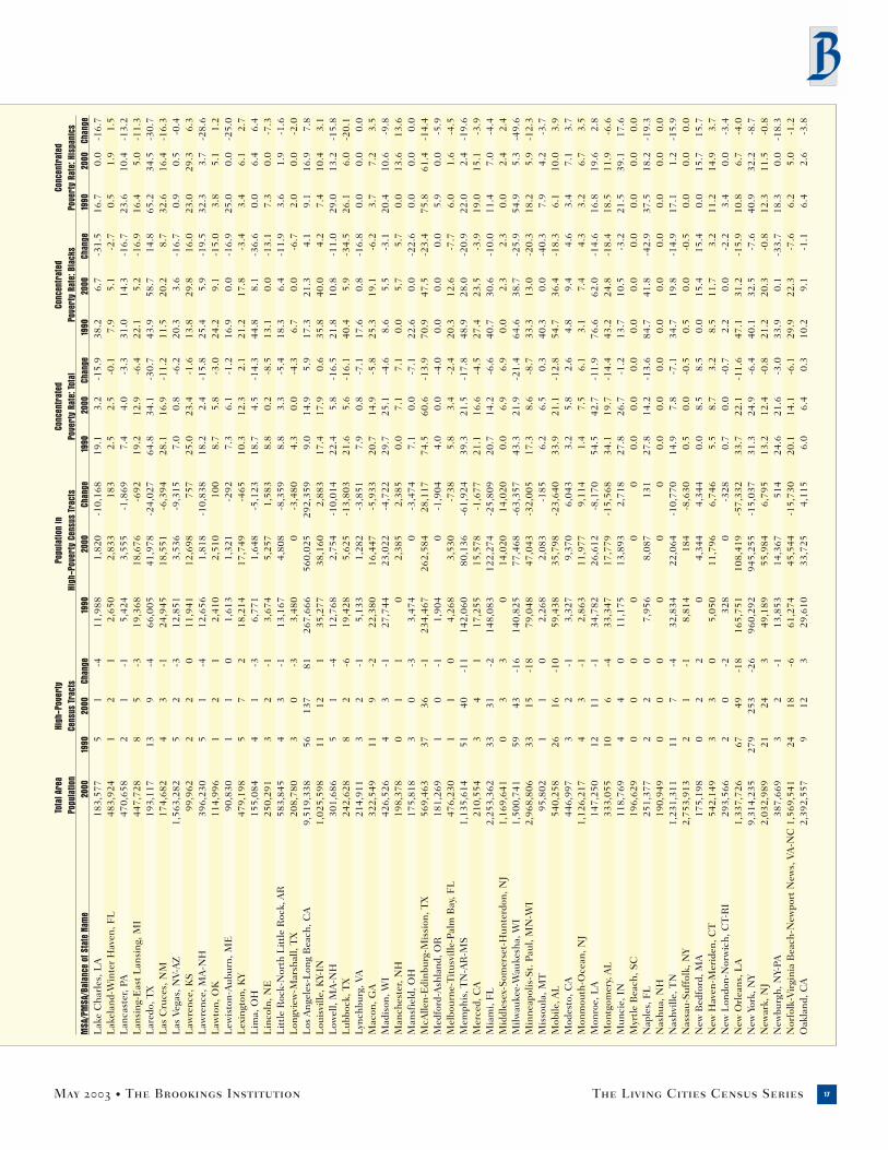
May 2003 • The Brookings Institution The Living Cities Census Series 17

Tota

l Are

aHi

gh-P

over

ty

Popu

latio

n in

Co

ncen

trat

ed

Conc

entr

ated

Co

ncen

trat

ed

Popu

latio

nCe

nsus

Trac

tsHi

gh-P

over

ty C

ensu

s Tr

acts

Pove

rty

Rate

: Tot

alPo

vert

y Ra

te: B

lack

sPo

vert

y Ra

te: H

ispa

nics

MSA

/PM

SA/B

alan

ce o

f Sta

te N

ame

2000

1990

2000

Chan

ge19

9020

00Ch

ange

1990

2000

Chan

ge19

9020

00Ch

ange

1990

2000

Chan

geL

ake

Cha

rles

, LA

183,

577

51

-411

,988

1,82

0-1

0,16

819

.13.

2-1

5.9

38.2

6.7

-31.

516

.70.

0-1

6.7

Lak

elan

d-W

inte

r H

aven

, FL

483,

924

12

12,

650

2,83

318

32.

52.

5-0

.17.

95.

1-2

.70.

51.

91.

5L

anca

ster

, PA

470,

658

21

-15,

424

3,55

5-1

,869

7.4

4.0

-3.3

31.0

14.3

-16.

723

.610

.4-1

3.2

Lan

sing

-Eas

t L

ansi

ng, M

I44

7,72

88

5-3

19,3

6818

,676

-692

19.2

12.9

-6.4

22.1

5.2

-16.

916

.45.

0-1

1.3

Lar

edo,

TX

193,

117

139

-466

,005

41,9

78-2

4,02

764

.834

.1-3

0.7

43.9

58.7

14.8

65.2

34.5

-30.

7L

as C

ruce

s, N

M17

4,68

24

3-1

24,9

4518

,551

-6,3

9428

.116

.9-1

1.2

11.5

20.2

8.7

32.6

16.4

-16.

3L

as V

egas

, NV-

AZ

1,56

3,28

25

2-3

12,8

513,

536

-9,3

157.

00.

8-6

.220

.33.

6-1

6.7

0.9

0.5

-0.4

Law

renc

e, K

S99

,962

22

011

,941

12,6

9875

725

.023

.4-1

.613

.829

.816

.023

.029

.36.

3L

awre

nce,

MA

-NH

396,

230

51

-412

,656

1,81

8-1

0,83

818

.22.

4-1

5.8

25.4

5.9

-19.

532

.33.

7-2

8.6

Law

ton,

OK

114,

996

12

12,

410

2,51

010

08.

75.

8-3

.024

.29.

1-1

5.0

3.8

5.1

1.2

Lew

isto

n-A

ubur

n, M

E90

,830

11

01,

613

1,32

1-2

927.

36.

1-1

.216

.90.

0-1

6.9

25.0

0.0

-25.

0L

exin

gton

, KY

479,

198

57

218

,214

17,7

49-4

6510

.312

.32.

121

.217

.8-3

.43.

46.

12.

7L

ima,

OH

155,

084

41

-36,

771

1,64

8-5

,123

18.7

4.5

-14.

344

.88.

1-3

6.6

0.0

6.4

6.4

Lin

coln

, NE

250,

291

32

-13,

674

5,25

71,

583

8.8

0.2

-8.5

13.1

0.0

-13.

17.

30.

0-7

.3L

ittl

e R

ock-

Nor

th L

ittl

e R

ock,

AR

583,

845

43

-113

,167

4,80

8-8

,359

8.8

3.3

-5.4

18.3

6.4

-11.

93.

61.

9-1

.6L

ongv

iew

-Mar

shal

l, T

X20

8,78

03

0-3

3,48

00

-3,4

804.

30.

0-4

.36.

70.

0-6

.72.

00.

0-2

.0L

os A

ngel

es-L

ong

Bea

ch, C

A9,

519,

338

5613

781

267,

666

560,

025

292,

359

9.0

14.9

5.9

17.3

21.3

4.1

9.1

16.9

7.8

Lou

isvi

lle, K

Y-IN

1,02

5,59

811

121

35,2

7738

,160

2,88

317

.417

.90.

635

.840

.04.

27.

410

.43.

1L

owel

l, M

A-N

H30

1,68

65

1-4

12,7

682,

754

-10,

014

22.4

5.8

-16.

521

.810

.8-1

1.0

29.0

13.2

-15.

8L

ubbo

ck, T

X24

2,62

88

2-6

19,4

285,

625

-13,

803

21.6

5.6

-16.

140

.45.

9-3

4.5

26.1

6.0

-20.

1Ly

nchb

urg,

VA

214,

911

32

-15,

133

1,28

2-3

,851

7.9

0.8

-7.1

17.6

0.8

-16.

80.

00.

00.

0M

acon

, GA

322,

549

119

-222

,380

16,4

47-5

,933

20.7

14.9

-5.8

25.3

19.1

-6.2

3.7

7.2

3.5

Mad

ison

, WI

426,

526

43

-127

,744

23,0

22-4

,722

29.7

25.1

-4.6

8.6

5.5

-3.1

20.4

10.6

-9.8

Man

ches

ter,

NH

198,

378

01

10

2,38

52,

385

0.0

7.1

7.1

0.0

5.7

5.7

0.0

13.6

13.6

Man

sfie

ld, O

H17

5,81

83

0-3

3,47

40

-3,4

747.

10.

0-7

.122

.60.

0-2

2.6

0.0

0.0

0.0

McA

llen-

Edi

nbur

g-M

issi

on, T

X56

9,46

337

36-1

234,

467

262,

584

28,1

1774

.560

.6-1

3.9

70.9

47.5

-23.

475

.861

.4-1

4.4

Med

ford

-Ash

land

, OR

181,

269

10

-11,

904

0-1

,904

4.0

0.0

-4.0

0.0

0.0

0.0

5.9

0.0

-5.9

Mel

bour

ne-T

itus

ville

-Pal

m B

ay, F

L47

6,23

01

10

4,26

83,

530

-738

5.8

3.4

-2.4

20.3

12.6

-7.7

6.0

1.6

-4.5

Mem

phis

, TN

-AR

-MS

1,13

5,61

451

40-1

114

2,06

080

,136

-61,

924

39.3

21.5

-17.

848

.928

.0-2

0.9

22.0

2.4

-19.

6M

erce

d, C

A21

0,55

43

41

17,2

5515

,578

-1,6

7721

.116

.6-4

.527

.423

.5-3

.919

.015

.1-3

.9M

iam

i, F

L2,

253,

362

3331

-214

8,08

312

2,27

4-2

5,80

920

.714

.2-6

.640

.730

.6-1

0.0

11.4

7.0

-4.4

Mid

dles

ex-S

omer

set-

Hun

terd

on, N

J1,

169,

641

03

30

14,0

2014

,020

0.0

6.9

6.9

0.0

2.3

2.3

0.0

2.4

2.4

Milw

auke

e-W

auke

sha,

WI

1,50

0,74

159

43-1

614

0,82

577

,468

-63,

357

43.3

21.9

-21.

464

.638

.7-2

5.9

54.9

5.3

-49.

6M

inne

apol

is-S

t. P

aul,

MN

-WI

2,96

8,80

633

15-1

879

,048

47,0

43-3

2,00

517

.38.

6-8

.733

.313

.0-2

0.3

18.2

5.9

-12.

3M

isso

ula,

MT

95,8

021

10

2,26

82,

083

-185

6.2

6.5

0.3

40.3

0.0

-40.

37.

94.

2-3

.7M

obile

, AL

540,

258

2616

-10

59,4

3835

,798

-23,

640

33.9

21.1

-12.

854

.736

.4-1

8.3

6.1

10.0

3.9

Mod

esto

, CA

446,

997

32

-13,

327

9,37

06,

043

3.2

5.8

2.6

4.8

9.4

4.6

3.4

7.1

3.7

Mon

mou

th-O

cean

, NJ

1,12

6,21

74

3-1

2,86

311

,977

9,11

41.

47.

56.

13.

17.

44.

33.

26.

73.

5M

onro

e, L

A14

7,25

012

11-1

34,7

8226

,612

-8,1

7054

.542

.7-1

1.9

76.6

62.0

-14.

616

.819

.62.

8M

ontg

omer

y, A

L33

3,05

510

6-4

33,3

4717

,779

-15,

568

34.1

19.7

-14.

443

.224

.8-1

8.4

18.5

11.9

-6.6

Mun

cie,

IN

118,

769

44

011

,175

13,8

932,

718

27.8

26.7

-1.2

13.7

10.5

-3.2

21.5

39.1

17.6

Myr

tle

Bea

ch, S

C19

6,62

90

00

00

00.

00.

00.

00.

00.

00.

00.

00.

00.

0N

aple

s, F

L25

1,37

72

20

7,95

68,

087

131

27.8

14.2

-13.

684

.741

.8-4

2.9

37.5

18.2

-19.

3N

ashu

a, N

H19

0,94

90

00

00

00.

00.

00.

00.

00.

00.

00.

00.

00.

0N

ashv

ille,

TN

1,23

1,31

111

7-4

32,8

3422

,064

-10,

770

14.9

7.8

-7.1

34.7

19.8

-14.

917

.11.

2-1

5.9

Nas

sau-

Suf

folk

, NY

2,75

3,91

32

1-1

8,81

418

4-8

,630

0.5

0.0

-0.5

0.5

0.0

-0.5

0.0

0.0

0.0

New

Bed

ford

, MA

175,

198

02

20

4,34

44,

344

0.0

8.5

8.5

0.0

15.4

15.4

0.0

15.7

15.7

New

Hav

en-M

erid

en, C

T54

2,14

93

30

5,05

011

,796

6,74

65.

58.

73.

28.

511

.73.

211

.214

.93.

7N

ew L

ondo

n-N

orw

ich,

CT-

RI

293,

566

20

-232

80

-328

0.7

0.0

-0.7

2.2

0.0

-2.2

3.4

0.0

-3.4

New

Orl

eans

, LA

1,33

7,72

667

49-1

816

5,75

110

8,41

9-5

7,33

233

.722

.1-1

1.6

47.1

31.2

-15.

910

.86.

7-4

.0N

ew Y

ork,

NY

9,31

4,23

527

925

3-2

696

0,29

294

5,25

5-1

5,03

731

.324

.9-6

.440

.132

.5-7

.640

.932

.2-8

.7N

ewar

k, N

J2,

032,

989

2124

349

,189

55,9

846,

795

13.2

12.4

-0.8

21.2

20.3

-0.8

12.3

11.5

-0.8

New

burg

h, N

Y-PA

387,

669

32

-113

,853

14,3

6751

424

.621

.6-3

.033

.90.

1-3

3.7

18.3

0.0

-18.

3N

orfo

lk-V

irgi

nia

Bea

ch-N

ewpo

rt N

ews,

VA

-NC

1,56

9,54

124

18-6

61,2

7445

,544

-15,

730

20.1

14.1

-6.1

29.9

22.3

-7.6

6.2

5.0

-1.2

Oak

land

, CA

2,39

2,55

79

123

29,6

1033

,725

4,11

56.

06.

40.

310

.29.

1-1

.16.

42.

6-3

.8

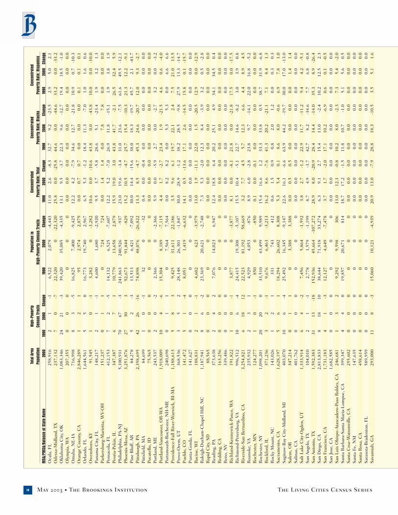
May 2003 • The Brookings Institution The Living Cities Census Series18

Tota

l Are

aHi

gh-P

over

ty

Popu

latio

n in

Co

ncen

trat

ed

Conc

entr

ated

Co

ncen

trat

ed

Popu

latio

nCe

nsus

Trac

tsHi

gh-P

over

ty C

ensu

s Tr

acts

Pove

rty

Rate

: Tot

alPo

vert

y Ra

te: B

lack

sPo

vert

y Ra

te: H

ispa

nics

MSA

/PM

SA/B

alan

ce o

f Sta

te N

ame

2000

1990

2000

Chan

ge19

9020

00Ch

ange

1990

2000

Chan

ge19

9020

00Ch

ange

1990

2000

Chan

geO

cala

, FL

258,

916

21

-16,

522

2,07

9-4

,443

11.0

2.6

-8.3

32.7

9.2

-23.

52.

95.

02.

1O

dess

a-M

idla

nd, T

X23

7,13

27

0-7

22,3

200

-22,

320

25.8

0.0

-25.

844

.60.

0-4

4.6

33.2

0.0

-33.

2O

klah

oma

Cit

y, O

K1,

083,

346

2421

-339

,420

35,0

85-4

,335

13.1

9.5

-3.7

22.3

9.6

-12.

719

.418

.5-1

.0O

lym

pia,

WA

207,

355

00

00

00

0.0

0.0

0.0

0.0

0.0

0.0

0.0

0.0

0.0

Om

aha,

NE

-IA

716,

998

83

-516

,825

7,40

0-9

,425

12.2

4.2

-7.9

34.6

12.7

-21.

810

.90.

7-1

0.3

Ora

nge

Cou

nty,

CA

2,84

6,28

91

21

952,

974

2,87

90.

00.

70.

70.

00.

00.

00.

10.

10.

1O

rlan

do, F

L1,

644,

561

55

016

,773

19,7

402,

967

6.5

5.3

-1.2

18.4

11.3

-7.0

1.0

1.6

0.6

Ow

ensb

oro,

KY

91,5

451

0-1

3,28

20

-3,2

8210

.60.

0-1

0.6

43.8

0.0

-43.

810

.00.

0-1

0.0

Pana

ma

Cit

y, F

L14

8,21

72

1-1

4,60

01,

680

-2,9

209.

53.

7-5

.828

.65.

1-2

3.4

1.9

3.2

1.3

Park

ersb

urg-

Mar

iett

a, W

V-O

H15

1,23

70

11

072

472

40.

01.

41.

40.

07.

87.

80.

00.

00.

0Pe

nsac

ola,

FL

412,

153

72

-514

,132

6,52

5-7

,607

12.2

5.2

-7.0

26.9

11.8

-15.

11.

93.

81.

9Pe

oria

-Pek

in, I

L34

7,38

76

71

10,7

7913

,658

2,87

915

.919

.03.

043

.841

.7-2

.126

.532

.45.

9P

hila

delp

hia,

PA

-NJ

5,10

0,93

170

67-3

241,

863

240,

926

-937

23.0

19.6

-3.4

31.0

23.6

-7.5

61.6

49.5

-12.

1P

hoen

ix-M

esa,

AZ

3,25

1,87

627

303

92,6

7391

,844

-829

15.2

10.5

-4.7

25.7

15.4

-10.

321

.312

.2-9

.1P

ine

Blu

ff, A

R84

,278

52

-313

,513

6,42

1-7

,092

30.0

14.4

-15.

638

.018

.3-1

9.7

45.7

2.1

-43.

7P

itts

burg

h, P

A2,

358,

695

4226

-16

74,8

9848

,076

-26,

822

13.3

8.5

-4.7

45.3

24.6

-20.

712

.09.

3-2

.7P

itts

fiel

d, M

A84

,699

10

-132

0-3

20.

40.

0-0

.40.

00.

00.

00.

00.

00.

0Po

cate

llo, I

D75

,565

00

00

00

0.0

0.0

0.0

0.0

0.0

0.0

0.0

0.0

0.0

Port

land

, ME

243,

537

20

-22,

366

0-2

,366

5.9

0.0

-5.9

2.7

0.0

-2.7

3.2

0.0

-3.2

Port

land

-Van

couv

er, O

R-W

A1,

918,

009

104

-615

,304

8,18

9-7

,115

4.4

1.7

-2.7

23.4

1.9

-21.

54.

60.

6-4

.0Po

rtsm

outh

-Roc

hest

er, N

H-M

E24

0,69

80

11

07,

564

7,56

40.

08.

28.

20.

05.

35.

30.

06.

66.

6P

rovi

denc

e-Fa

ll R

iver

-War

wic

k, R

I-M

A1,

188,

613

58

39,

425

31,6

1122

,186

3.5

9.6

6.1

19.7

22.1

2.4

7.5

21.0

13.5

Pro

vo-O

rem

, UT

368,

536

35

228

,148

26,3

01-1

,847

30.0

28.9

-1.2

38.2

28.5

-9.8

27.9

13.3

-14.

7P

uebl

o, C

O14

1,47

25

1-4

8,05

11,

419

-6,6

3214

.10.

5-1

3.6

17.1

2.6

-14.

515

.80.

1-1

5.7

Pun

ta G

orda

, FL

141,

627

00

00

00

0.0

0.0

0.0

0.0

0.0

0.0

0.0

0.0

0.0

Rac

ine,

WI

188,

831

21

-14,

602

623

-3,9

7913

.01.

9-1

1.1

22.0

1.5

-20.

512

.90.

0-1

2.9

Ral

eigh

-Dur

ham

-Cha

pel H

ill, N

C1,

187,

941

86

-223

,369

20,6

21-2

,748

7.3

5.3

-2.0

12.3

8.4

-3.9

3.2

0.5

-2.8

Rap

id C

ity,

SD

88,5

650

00

00

00.

00.

00.

00.

00.

00.

00.

00.

00.

0R

eadi

ng, P

A37

3,63

82

42

7,07

614

,023

6,94

712

.418

.86.

420

.225

.14.

934

.134

.50.

4R

eddi

ng, C

A16

3,25

60

00

00

00.

00.

00.

00.

00.

00.

00.

00.

00.

0R

eno,

NV

339,

486

00

00

00

0.0

0.0

0.0

0.0

0.0

0.0

0.0

0.0

0.0

Ric

hlan

d-K

enne

wic

k-Pa

sco,

WA

191,

822

10

-13,

877

0-3

,877

8.1

0.0

-8.1

21.8

0.0

-21.

817

.50.

0-1

7.5

Ric

hmon

d-Pe

ters

burg

, VA

996,

512

106

-424

,415

19,3

08-5

,107

15.5

10.4

-5.1

22.7

14.6

-8.2

3.0

3.9

0.8

Riv

ersi

de-S

an B

erna

rdin

o, C

A3,

254,

821

618

1222

,523

81,1

9258

,669

3.2

7.7

4.5

5.7

12.3

6.6

4.4

8.9

4.5

Roa

noke

, VA

235,

932

23

14,

929

4,05

3-8

768.

96.

0-2

.823

.89.

7-1

4.1

22.0

16.8

-5.2

Roc

hest

er, M

N12

4,27

71

0-1

850

0-8

500.

10.

0-0

.10.

00.

00.

00.

00.

00.

0R

oche

ster

, NY

1,09

8,20

120

200

33,5

1043

,499

9,98

915

.416

.61.

233

.333

.80.

538

.731

.9-6

.8R

ockf

ord,

IL

371,

236

32

-19,

676

6,46

3-3

,213

16.2

8.6

-7.6

41.3

20.2

-21.

17.

18.

41.

3R

ocky

Mou

nt, N

C14

3,02

61

21

331

743

412

0.6

1.5

0.9

0.8

2.0

1.2

0.0

0.3

0.3

Sac

ram

ento

, CA

1,62

8,19

75

61

18,2

9426

,602

8,30

85.

35.

40.

18.

68.

0-0

.66.

97.

81.

0S

agin

aw-B

ay C

ity-

Mid

land

, MI

403,

070

106

-425

,492

16,3

45-9

,147

22.6

16.1

-6.6

63.9

44.2

-19.

730

.017

.0-1

3.0

Sal

em, O

R34

7,21

40

11

03,

388

3,38

80.

00.

50.

50.

00.

00.

00.

01.

41.

4S

alin

as, C

A40

1,76

20

00

00

00.

00.

00.

00.

00.

00.

00.

00.

00.

0S

alt

Lak

e C

ity-

Ogd

en, U

T1,

333,

914

64

-27,

456

5,86

4-1

,592

3.8

2.7

-1.2

22.9

11.7

-11.

29.

44.

2-5

.1S

an A

ngel

o, T

X10

4,01

02

1-1

2,77

81,

579

-1,1

998.

74.

9-3

.742

.78.

2-3

4.6

7.7

6.8

-0.8

San

Ant

onio

, TX

1,59

2,38

331

13-1

815

2,93

645

,664

-107

,272

28.9

8.0

-20.

928

.414

.4-1

4.0

35.3

8.9

-26.

4S

an D

iego

, CA

2,81

3,83

38

1810

38,6

4471

,918

33,2

746.

39.

12.

715

.413

.0-2

.410

.212

.52.

3S

an F

ranc

isco

, CA

1,73

1,18

34

1-3

12,1

274,

649

-7,4

783.

71.

7-2

.017

.110

.2-6

.90.

60.

1-0

.5S

an J

ose,

CA

1,68

2,58

50

00

00

00.

00.

00.

00.

00.

00.

00.

00.

00.

0S

an L

uis

Obi

spo-

Ata

scad

ero-

Paso

Rob

les,

CA

246,

681

13

29,

292

9,59

830

613

.012

.1-0

.810

.28.

0-2

.37.

35.

4-2

.0S

anta

Bar

bara

-San

ta M

aria

-Lom

poc,

CA

399,

347

44

019

,857

20,6

7181

418

.717

.2-1

.511

.810

.7-1

.05.

15.

60.

5S

anta

Cru

z-W

atso

nvill

e, C

A25

5,60

20

00

00

00.

00.

00.

00.

00.

00.

00.

00.

00.

0S

anta

Fe,

NM

147,

635

00

00

00

0.0

0.0

0.0

0.0

0.0

0.0

0.0

0.0

0.0

San

ta R

osa,

CA

458,

614

00

00

00

0.0

0.0

0.0

0.0

0.0

0.0

0.0

0.0

0.0

Sar

asot

a-B

rade

nton

, FL

589,

959

00

00

00

0.0

0.0

0.0

0.0

0.0

0.0

0.0

0.0

0.0

Sav

anna

h, G

A29

3,00

011

8-3

15,0

6010

,121

-4,9

3920

.913

.0-7

.928

.818

.3-1

0.5

3.5

5.1

1.6

May 2003 • The Brookings Institution The Living Cities Census Series 19

Tota

l Are

aHi

gh-P

over

ty

Popu

latio

n in

Co

ncen

trat

ed

Conc

entr

ated

Co

ncen

trat

ed

Popu

latio

nCe

nsus

Trac

tsHi

gh-P

over

ty C

ensu

s Tr

acts

Pove

rty

Rate

: Tot

alPo

vert

y Ra

te: B

lack

sPo

vert

y Ra

te: H

ispa

nics

MSA

/PM

SA/B

alan

ce o

f Sta

te N

ame

2000

1990

2000

Chan

ge19

9020

00Ch

ange

1990

2000

Chan

ge19

9020

00Ch

ange

1990

2000

Chan

geS

cran

ton—

Wilk

es-B

arre

—H

azle

ton,

PA

624,

776

22

03,

483

8,56

85,

085

2.2

3.7

1.5

13.1

6.6

-6.5

0.0

5.9

5.9

Sea

ttle

-Bel

levu

e-E

vere

tt, W

A2,

414,

616

94

-524

,775

14,6

46-1

0,12

95.

02.

4-2

.66.

83.

4-3

.38.

11.

3-6

.8S

haro

n, P

A12

0,29

33

2-1

4,36

32,

407

-1,9

5613

.58.

7-4

.761

.831

.6-3

0.2

21.3

47.1

25.8

She

boyg

an, W

I11

2,64

60

00

00

00.

00.

00.

00.

00.

00.

00.

00.

00.

0S

herm

an-D

enis

on, T

X11

0,59

51

0-1

325

0-3

251.

20.

0-1

.22.

80.

0-2

.84.

00.

0-4

.0S

hrev

epor

t-B

ossi

er C

ity,

LA

392,

302

1818

059

,130

40,7

41-1

8,38

935

.425

.2-1

0.2

47.0

32.0

-15.

015

.217

.11.

9S

ioux

Cit

y, I

A-N

E12

4,13

02

1-1

4,51

751

-4,4

6613

.60.

2-1

3.3

27.6

0.0

-27.

625

.00.

6-2

4.4

Sio

ux F

alls

, SD

172,

412

10

-11,

252

0-1

,252

5.2

0.0

-5.2

4.7

0.0

-4.7

0.0

0.0

0.0

Sou

th B

end,

IN

265,

559

10

-11,

525

0-1

,525

3.0

0.0

-3.0

7.1

0.0

-7.1

3.1

0.0

-3.1

Spo

kane

, WA

417,

939

61

-56,

766

2,20

3-4

,563

5.9

2.0

-3.8

5.9

4.3

-1.5

4.9

1.7

-3.1

Spr

ingf

ield

, IL

201,

437

21

-14,

000

1,81

8-2

,182

10.8

5.9

-5.0

28.4

13.9

-14.

60.

00.

00.

0S

prin

gfie

ld, M

A59

1,93

211

110

43,8

1434

,957

-8,8

5728

.721

.7-7

.039

.921

.6-1

8.3

59.1

43.2

-15.

9S

prin

gfie

ld, M

O32

5,72

14

2-2

13,1

636,

046

-7,1

1711

.23.

6-7

.631

.54.

6-2

6.9

10.9

7.1

-3.8

St.

Clo

ud, M

N16

7,39

23

1-2

12,1

721,

102

-11,

070

22.9

1.1

-21.

86.

53.

2-3

.219

.81.

0-1

8.8

St.

Jos

eph,

MO

102,

490

20

-24,

132

0-4

,132

12.7

0.0

-12.

739

.50.

0-3

9.5

3.5

0.0

-3.5

St.

Lou

is, M

O-I

L2,

603,

607

3926

-13

109,

516

70,6

50-3

8,86

620

.513

.0-7

.539

.123

.8-1

5.3

12.8

5.2

-7.6

Sta

mfo

rd-N

orw

alk,

CT

353,

556

00

00

00

0.0

0.0

0.0

0.0

0.0

0.0

0.0

0.0

0.0

Sta

te C

olle

ge, P

A13

5,75

85

61

23,6

7928

,955

5,27

652

.149

.5-2

.654

.536

.6-1

7.9

28.6

55.1

26.5

Ste

uben

ville

-Wei

rton

, OH

-WV

132,

008

42

-25,

756

3,33

0-2

,426

12.5

8.2

-4.4

57.6

33.9

-23.

77.

813

.96.

1S

tock

ton-

Lod

i, C

A56

3,59

85

72

25,8

5834

,504

8,64

615

.215

.50.

322

.324

.42.

118

.115

.7-2

.4S

umte

r, S

C10

4,64

63

0-3

10,5

450

-10,

545

22.1

0.0

-22.

127

.30.

0-2

7.3

0.0

0.0

0.0

Syr

acus

e, N

Y73

2,11

714

12-2

38,1

5034

,670

-3,4

8020

.416

.9-3

.556

.542

.0-1

4.5

48.1

46.5

-1.5

Taco

ma,

WA

700,

820

53

-212

,688

8,18

0-4

,508

10.0

4.7

-5.4

16.5

7.3

-9.2

6.8

1.9

-4.8

Talla

hass

ee, F

L28

4,53

910

9-1

36,0

3643

,439

7,40

334

.239

.85.

633

.334

.20.

938

.241

.83.

7Ta

mpa

-St.

Pet

ersb

urg-

Cle

arw

ater

, FL

2,39

5,99

716

11-5

40,9

5629

,465

-11,

491

9.1

5.5

-3.5

29.1

17.8

-11.

47.

34.

7-2

.6Te

rre

Hau

te, I

N14

9,19

22

20

3,00

65,

501

2,49

56.

55.

9-0

.59.

719

.910

.210

.03.

9-6

.1Te

xark

ana,

TX

-Tex

arka

na, A

R12

9,74

92

31

4,58

78,

327

3,74

012

.216

.24.

023

.828

.64.

80.

011

.611

.6To

ledo

, OH

618,

203

209

-11

53,3

9223

,381

-30,

011

25.1

10.6

-14.

537

.218

.8-1

8.4

28.2

9.0

-19.

1To

peka

, KS

169,

871

00

00

00

0.0

0.0

0.0

0.0

0.0

0.0

0.0

0.0

0.0

Tren

ton,

NJ

350,

761

12

15,

110

4,82

9-2

817.

97.

6-0

.38.

410

.42.

025

.112

.1-1

3.0

Tucs

on, A

Z84

3,74

613

8-5

52,8

7928

,962

-23,

917

21.1

8.5

-12.

622

.03.

5-1

8.6

22.6

5.9

-16.

7Tu

lsa,

OK

803,

235

116

-529

,066

14,3

28-1

4,73

813

.36.

7-6

.535

.218

.8-1

6.3

12.1

4.2

-7.9

Tusc

aloo

sa, A

L16

4,87

56

3-3

26,9

8810

,712

-16,

276

34.6

16.1

-18.

537

.06.

1-3

0.9

49.5

16.9

-32.

6Ty

ler,

TX

174,

706

40

-410

,105

0-1

0,10

518

.10.

0-1

8.1

29.3

0.0

-29.

330

.00.

0-3

0.0

Uti

ca-R

ome,

NY

299,

896

46

23,

094

9,16

56,

071

4.6

10.7

6.2

20.4

37.1

16.7

6.2

14.4

8.3

Valle

jo-F

airf

ield

-Nap

a, C

A51

8,82

11

10

961,

096

1,00

00.

20.

20.

00.

00.

30.

30.

80.

1-0

.7Ve

ntur

a, C

A75

3,19

70

00

00

00.

00.

00.

00.

00.

00.

00.

00.

00.

0V

icto

ria,

TX

84,0

882

0-2

4,37

30

-4,3

7315

.60.

0-1

5.6

29.8

0.0

-29.

817

.80.

0-1

7.8

Vin

elan

d-M

illvi

lle-B

ridg

eton

, NJ

146,

438

00

00

00

0.0

0.0

0.0

0.0

0.0

0.0

0.0

0.0

0.0

Vis

alia

-Tul

are-

Port

ervi

lle, C

A36

8,02

14

62

18,6

0629

,782

11,1

7611

.614

.42.

87.

512

.34.

811

.715

.74.

0W

aco,

TX

213,

517

97

-233

,038

24,6

95-8

,343

40.8

30.8

-10.

057

.023

.9-3

3.2

28.4

23.5

-4.9

Was

hing

ton,

DC

-MD

-VA

-WV

4,92

3,15

310

2414

20,6

0977

,563

56,9

543.

37.

64.

36.

315

.08.

71.

00.

4-0

.6W

ater

bury

, CT

228,

984

11

025

34,

788

4,53

50.

79.

18.

40.

79.

58.

81.

012

.911

.9W

ater

loo-

Ced

ar F

alls

, IA

128,

012

21

-13,

461

8,17

04,

709

9.3

11.1

1.8

25.4

0.1

-25.

318

.32.

5-1

5.8

Wau

sau,

WI

125,

834

00

00

00

0.0

0.0

0.0

0.0

0.0

0.0

0.0

0.0

0.0

Wes

t Pa

lm B

each

-Boc

a R

aton

, FL

1,13

1,18

46

71

16,0

1819

,762

3,74

49.

07.

8-1

.221

.819

.2-2

.53.

33.

1-0

.2W

heel

ing,

WV-

OH

153,

172

03

30

3,06

63,

066

0.0

6.3

6.3

0.0

33.5

33.5

0.0

14.0

14.0

Wic

hita

Fal

ls, T

X14

0,51

86

0-6

8,39

80

-8,3

9820

.50.

0-2

0.5

59.1

0.0

-59.

127

.50.

0-2

7.5

Wic

hita

, KS

545,

220

62

-415

,104

5,59

8-9

,506

13.3

4.9

-8.4

36.3

10.6

-25.

810

.53.

0-7

.5W

illia

msp

ort,

PA

120,

044

11

02,

326

2,14

0-1

868.

76.

1-2

.717

.08.

6-8

.50.

00.

00.

0W

ilmin

gton

, NC

233,

450

52

-39,

120

4,31

7-4

,803

17.5

6.2

-11.

336

.816

.5-2

0.3

7.5

6.3

-1.2

Wilm

ingt

on-N

ewar

k, D

E-M

D58

6,21

63

52

4,47

016

,819

12,3

495.

313

.48.

113

.218

.04.

81.

312

.611

.3W

orce

ster

, MA

-CT

511,

389

45

18,

413

8,58

517

210

.27.

9-2

.321

.89.

2-1

2.6

28.4

19.6

-8.8

Yaki

ma,

WA

222,

581

42

-221

,179

12,4

39-8

,740

23.5

11.5

-12.

032

.517

.7-1

4.8

24.5

13.6

-10.

9Yo

lo, C

A16

8,66

01

10

6,33

06,

619

289

8.6

6.1

-2.5

2.8

4.8

2.0

3.6

2.2

-1.3

York

, PA

381,

751

00

00

00

0.0

0.0

0.0

0.0

0.0

0.0

0.0

0.0

0.0

May 2003 • The Brookings Institution The Living Cities Census Series20

Tota

l Are

aHi

gh-P

over

ty

Popu

latio

n in

Co

ncen

trat

ed

Conc

entr

ated

Co

ncen

trat

ed

Popu

latio

nCe

nsus

Trac

tsHi

gh-P

over

ty C

ensu

s Tr

acts

Pove

rty

Rate

: Tot

alPo

vert

y Ra

te: B

lack

sPo

vert

y Ra

te: H

ispa

nics

MSA

/PM

SA/B

alan

ce o

f Sta

te N

ame

2000

1990

2000

Chan

ge19

9020

00Ch

ange

1990

2000

Chan

ge19

9020

00Ch

ange

1990

2000

Chan

geYo

ungs

tow

n-W

arre

n, O

H59

4,74

619

6-1

335

,651

7,58

2-2

8,06

920

.24.

3-1

5.8

51.7

11.2

-40.

549

.23.

6-4

5.6

Yuba

Cit

y, C

A13

9,14

90

00

00

00.

00.

00.

00.

00.

00.

00.

00.

00.

0Yu

ma,

AZ

160,

026

31

-29,

574

4,71

3-4

,861

19.6

7.3

-12.

315

.514

.4-1

.124

.08.

9-1

5.0

Non

-Met

ropo

litan

Are

as in

Ala

bam

a1,

338,

141

3314

-19

102,

111

43,7

46-5

8,36

517

.16.

9-1

0.2

31.6

13.2

-18.

420

.32.

7-1

7.7

Non

-Met

ropo

litan

Are

as in

Ala

ska

366,

649

10

-11,

522

0-1

,522

1.9

0.0

-1.9

0.4

0.0

-0.4

0.0

0.0

0.0

Non

-Met

ropo

litan

Are

as in

Ari

zona

603,

632

2219

-391

,119

81,9

34-9

,185

45.1

32.1

-12.

910

.07.

8-2

.218

.69.

2-9

.5N

on-M

etro

polit

an A

reas

in A

rkan

sas

1,35

2,38

122

6-1

694

,024

25,4

90-6

8,53

415

.64.

2-1

1.3

37.4

11.4

-26.

014

.30.

6-1

3.7

Non

-Met

ropo

litan

Are

as in

Cal

ifor

nia

1,12

1,25

43

30

9,20

715

,553

6,34

62.

73.

60.

912

.210

.3-1

.93.

45.

72.

3N

on-M

etro

polit

an A

reas

in C

olor

ado

693,

605

40

-45,

043

0-5

,043

2.9

0.0

-2.9

4.1

0.0

-4.1

6.2

0.0

-6.2

Non

-Met

ropo

litan

Are

as in

Con

nect

icut

148,

665

00

00

00

0.0

0.0

0.0

0.0

0.0

0.0

0.0

0.0

0.0

Non

-Met

ropo

litan

Are

as in

Del

awar

e15

6,63

80

00

00

00.

00.

00.

00.

00.

00.

00.

00.

00.

0N

on-M

etro

polit

an A

reas

in F

lori

da1,

144,

881

21

-14,

831

3,90

8-9

231.

50.

9-0

.64.

73.

4-1

.20.

40.

2-0

.2N

on-M

etro

polit

an A

reas

in G

eorg

ia2,

519,

789

1313

052

,027

48,3

03-3

,724

5.4

5.2

-0.3

8.2

8.4

0.2

2.9

2.6

-0.3

Non

-Met

ropo

litan

Are

as in

Haw

aii

335,

381

21

-137

014

7-2

230.

60.

1-0

.40.

00.

00.

00.

40.

0-0

.4N

on-M

etro

polit

an A

reas

in I

daho

786,

043

22

011

,443

10,9

77-4

665.

65.

70.

16.

11.

8-4

.31.

21.

2-0

.1N

on-M

etro

polit

an A

reas

in I

llino

is1,

877,

585

97

-241

,191

23,3

61-1

7,83

05.

35.

0-0

.418

.611

.7-6

.87.

04.

9-2

.1N

on-M

etro

polit

an A

reas

in I

ndia

na1,

690,

582

10

-11,

028

0-1

,028

0.3

0.0

-0.3

5.3

0.0

-5.3

0.4

0.0

-0.4

Non

-Met

ropo

litan

Are

as in

Iow

a1,

600,

191

31

-212

,678

3,30

7-9

,371

2.5

1.0

-1.4

7.3

0.9

-6.3

4.6

0.3

-4.4

Non

-Met

ropo

litan

Are

as in

Kan

sas

1,16

7,35

52

31

9,02

712

,203

3,17

61.

93.

21.

33.

22.

0-1

.21.

11.

10.

0N

on-M

etro

polit

an A

reas

in K

entu

cky

2,06

8,66

752

15-3

713

6,28

336

,732

-99,

551

13.6

4.1

-9.5

9.5

0.5

-9.1

7.0

1.5

-5.4

Non

-Met

ropo

litan

Are

as in

Lou

isia

na1,

098,

766

4320

-23

175,

906

76,4

85-9

9,42

127

.313

.2-1

4.1

40.0

20.9

-19.

113

.87.

4-6

.4N

on-M

etro

polit

an A

reas

in M

aine

808,

317

10

-115

0-1

50.

00.

00.

00.

00.

00.

00.

00.

00.

0N

on-M

etro

polit

an A

reas

in M

aryl

and

385,

446

10

-11,

595

0-1

,595

1.7

0.0

-1.7

4.0

0.0

-4.0

5.5

0.0

-5.5

Non

-Met

ropo

litan

Are

as in

Mas

sach

uset

ts24

7,67

20

00

00

00.

00.

00.

00.

00.

00.

00.

00.

00.

0N

on-M

etro

polit

an A

reas

in M

ichi

gan

1,76

8,97

810

4-6

34,5

6220

,761

-13,

801

4.7

3.1

-1.6

11.7

10.0

-1.8

2.8

1.7

-1.1

Non

-Met

ropo

litan

Are

as in

Min

neso

ta1,

456,

119

22

011

,363

11,0

72-2

912.

32.

50.

34.

36.

32.

00.

60.

4-0

.2N

on-M

etro

polit

an A

reas

in M

issi

ssip

pi1,

820,

996

7730

-47

315,

974

120,

899

-195

,075

31.2

13.4

-17.

841

.919

.2-2

2.7

28.3

7.8

-20.

4N

on-M

etro

polit

an A

reas

in M

isso

uri

1,80

0,41

08

4-4

21,5

4614

,898

-6,6

483.

11.

7-1

.316

.68.

2-8

.41.

81.

3-0

.5N

on-M

etro

polit

an A

reas

in M

onta

na59

6,68

47

81

19,5

0012

,161

-7,3

3910

.06.

0-4

.02.

90.

0-2

.98.

74.

0-4

.6N

on-M

etro

polit

an A

reas

in N

ebra

ska

811,

425

01

10

4747

0.0

0.0

0.0

0.0

0.0

0.0

0.0

0.0

0.0

Non

-Met

ropo

litan

Are

as in

Nev

ada

250,

521

00

00

00

0.0

0.0

0.0

0.0

0.0

0.0

0.0

0.0

0.0

Non

-Met

ropo

litan

Are

as in

New

Ham

pshi

re49

6,08

70

00

00

00.

00.

00.

00.

00.

00.

00.

00.

00.

0N

on-M

etro

polit

an A

reas

in N

ew M

exic

o78

3,99

129

15-1

490

,945

52,4

03-3

8,54

227

.914

.2-1

3.7

21.7

6.7

-15.

09.

63.

1-6

.5N

on-M

etro

polit

an A

reas

in N

ew Y

ork

1,50

3,39

99

4-5

20,9

0010

,692

-10,

208

2.8

2.7

-0.1

1.8

2.0

0.1

4.4

2.1

-2.3

Non

-Met

ropo

litan

Are

as in

Nor

th C

arol

ina

2,61

2,25

710

6-4

35,0

1218

,136

-16,

876

4.0

2.1

-2.0

7.3

4.2

-3.1

1.9

1.6

-0.3

Non

-Met

ropo

litan

Are

as in

Nor

th D

akot

a35

8,23

46

3-3

18,1

001,

059

-17,

041

14.3

1.1

-13.

10.

01.

61.

68.

20.

6-7

.6N

on-M

etro

polit

an A

reas

in O

hio

2,13

9,36

43

41

19,1

8615

,620

-3,5

662.

42.

40.

01.

91.

90.

13.

41.

0-2

.4N

on-M

etro

polit

an A

reas

in O

klah

oma

1,35

2,29

215

3-1

234

,710

9,12

4-2

5,58

65.

51.

2-4

.321

.83.

7-1

8.1

10.0

0.2

-9.8

Non

-Met

ropo

litan

Are

as in

Ore

gon

919,

033

00

00

00

0.0

0.0

0.0

0.0

0.0

0.0

0.0

0.0

0.0

Non

-Met

ropo

litan

Are

as in

Pen

nsyl

vani

a1,

889,

525

24

212

,497

18,5

766,

079

1.8

3.2

1.4

17.8

13.8

-4.0

0.4

2.1

1.7

Non

-Met

ropo

litan

Are

as in

Rho

de I

slan

d61

,968

00

00

00

0.0

0.0

0.0

0.0

0.0

0.0

0.0

0.0

0.0

Non

-Met

ropo

litan

Are

as in

Sou

th C

arol

ina

1,20

5,05

04

1-3

10,4

452,

570

-7,8

752.

20.

6-1

.62.

50.

9-1

.60.

70.

0-0

.7N

on-M

etro

polit

an A

reas

in S

outh

Dak

ota

493,

867

1119

838

,227

30,2

57-7

,970

22.6

21.4

-1.2

11.5

11.5

-0.1

24.1

11.8

-12.

3N

on-M

etro

polit

an A

reas

in T

enne

ssee

1,82

7,13

95

2-3

5,93

15,

260

-671

0.9

0.8

-0.1

0.0

0.9

0.9

1.9

2.6

0.6

Non

-Met

ropo

litan

Are

as in

Tex

as3,

159,

940

5126

-25

210,

746

109,

885

-100

,861

16.0

9.0

-7.0

7.0

6.5

-0.5

32.6

16.5

-16.

1N

on-M

etro

polit

an A

reas

in U

tah

524,

673

14

33,

495

17,7

0914

,214

4.1

11.9

7.7

0.0

12.5

12.5

0.8

2.1

1.3

Non

-Met

ropo

litan

Are

as in

Ver

mon

t43

9,43

61

0-1

70

-70.

00.

00.

00.

00.

00.

00.

00.

00.

0N

on-M

etro

polit

an A

reas

in V

irgi

nia

1,55

0,44

74

3-1

22,2

5822

,778

520

2.9

6.2

3.3

0.2

1.0

0.8

11.0

4.3

-6.7

Non

-Met

ropo

litan

Are

as in

Was

hing

ton

994,

967

54

-117

,111

18,0

5194

04.

75.

20.

523

.415

.3-8

.14.

51.

6-2

.9N

on-M

etro

polit

an A

reas

in W

est

Vir

gini

a1,

042,

776

106

-433

,300

19,6

36-1

3,66

45.

54.

0-1

.410

.33.

6-6

.77.

25.

0-2

.2N

on-M

etro

polit

an A

reas

in W

isco

nsin

1,72

3,36

74

0-4

12,6

760

-12,

676

2.9

0.0

-2.9

1.0

0.0

-1.0

1.4

0.0

-1.4

Non

-Met

ropo

litan

Are

as in

Wyo

min

g34

5,64

22

1-1

7,41

23,

345

-4,0

678.

11.

5-6

.60.

016

.616

.62.

00.

3-1

.6

U.S

. Tot

al28

1,42

1,90

63,

417

2,51

0-9

0710

,393

,954

7,94

6,29

1-2

,447

,663

15.1

10.3

-4.8

30.4

18.6

-11.

821

.213

.8-7

.4

May 2003 • The Brookings Institution The Living Cities Census Series 21

References

Danziger, Sheldon H. and PeterGottschalk. 1987. “Earnings Inequal-ity, the Spatial Concentration ofPoverty, and the Underclass.” Ameri-can Economic Review 77: 211–15.

Fisher, Gordon M. 1992. “The Devel-opment and History of the PovertyThresholds,” Social Security Bulletin55: 3–14.

Jargowsky, Paul A. 1997. Poverty andPlace: Ghettos, Barrios, and the Ameri-can City. New York: Russell SageFoundation.

Jargowsky, Paul A. and Mary Jo Bane.1990. “Ghetto Poverty: Basic Ques-tions.” In Inner-City Poverty in theUnited States, edited by L. E. Lynnand M. G. H. McGeary. Washington:National Academy Press.

Kasarda, John D. 1993. “Inner-CityPoverty and Economic Access.” In J.Sommer and D. A. Hicks, eds., Redis-covering Urban America: Perspectiveson the 1980s. U.S. Department ofHousing and Urban Development.

Orfield, Myron. 1996. Metropolitics: A Regional Agenda for Community and Stability. Washington: BrookingsInstitution Press.

——— . 2002. American Metropoli-tics: The New Suburban Reality. Wash-ington: Brookings Institution Press.

Orshansky, Mollie. 1965. “Countingthe Poor: Another Look at the PovertyProfile,” Social Security Bulletin 28:3–29.

Ruggles, Patricia. 1990. Drawing theLine: Alternative Poverty Measures andTheir Implications for Public Policy.Washington: Urban Institute Press.

Wilson, William Julius. 1987. TheTruly Disadvantaged: The Inner-City,the Underclass and Public Policy.Chicago: University of Chicago Press.

Endnotes

1. Paul Jargowsky directs the Bruton Centerfor Development Studies at the Universityof Texas at Dallas, and is associate profes-sor of political economy there. He is also aSenior Research Affiliate at the NationalPoverty Center at the University of Michi-gan. He is the author of Poverty and Place:Ghettos, Barrios, and the American City(New York: Russell Sage Foundation,1997).

2. For a thorough discussion of the trends inconcentrated poverty between 1970 and1990, see Jargowsky (1997), especiallychapter 2.

3. Patricia Ruggles, Drawing the Line: Alter-native Poverty Measures and Their Implica-tions for Public Policy (Washington: UrbanInstitute Press, 1990).

4. This is known as the Modifiable Areal UnitProblem, and has been studied extensivelyby geographers. See S. Openshaw and P.J.Taylor, “The Modifiable Areal Unit Prob-lem.” In N. Wrigley and R.J. Bennett, eds.,Quantitative Geography: A British View(London: Routledge, 1981).

5. Sheldon H. Danziger and Peter Gottschalk,“Earnings Inequality, the Spatial Concen-tration of Poverty, and the Underclass,”American Economic Review 77 (1987):211–15; Paul A. Jargowsky and Mary JoBane, “Ghetto Poverty: Basic Questions.”In L. E. Lynn and M. G. H. McGeary, eds.,Inner-City Poverty in the United States(Washington: National Academy Press,1991); John D. Kasarda, “Inner-CityPoverty and Economic Access.” In J. Som-mer and D. A. Hicks, eds., RediscoveringUrban America: Perspectives on the 1980s(U.S. Department of Housing and UrbanDevelopment, 1993).

6. In New England, metropolitan areas arebuilt up from subdivisions of countiesrather than whole counties. The CensusBureau also defines New England CountyMetropolitan Areas (NECMAs), which arecomposed of whole counties.

7. New England County Metropolitan Areas(NECMAs) are not considered for thesame reasons. Non-metropolitan areaswere first completely divided into censustracts in 1990, so Census 2000 providesthe first opportunity to conduct a trulynationwide study of the trends in concen-trated poverty. For presentation purposes,non-metropolitan neighborhoods aregrouped by state, but it should be notedthat these areas are residuals and may ormay not be contiguous.

8. In New England, census tracts can evencross metropolitan area boundaries.

9. The data in Figure 1 are for metropolitanareas only, as they existed at the time ofeach census. Nationwide data on neighbor-hood poverty are not available prior to1990, because census tracts in non-metro-politan areas were defined for the first timewith the release of the 1990 census.

10. Exceptions included metro areas such asAkron, Cleveland, Pittsburgh, andYoungstown, which despite double-digitdecreases in the number of high-povertyneighborhoods had declines of less than30,000 people living in such neighbor-hoods.

11. A technical note regarding the maps: Formapping purposes, a consistent set of cen-sus tract boundaries is employed. That way,it is possible to show how different areaschanged over time. However, for calculat-ing statistics, it is important to have a con-sistent neighborhood size over time. This isbest achieved by using contemporaneoustracts. In view of that, there is not an exactcorrespondence between the data used forthe maps and the data used for the tablesand figures presented in the text. For 1990and earlier years, these maps use datainterpolated to the 2000 census tract gridby the Urban Institute and Geolytics, Inc.

12. Robert E. Lang and Patrick A. Simmons,“Boomburbs: The Emergence of Large,Fast-Growing Suburban Cities.” In BruceKatz and Robert E. Lang, eds., RedefiningUrban and Suburban America: Evidencefrom Census 2000 (Washington: BrookingsInstitution Press, 2003).

13. During the 1990s, Los Angeles County lostsignificant white population, at the sametime that its Hispanic population grew bynearly 900,000.

14. William Julius Wilson, The Truly Disadvan-taged: The Inner-City, the Underclass andPublic Policy (University of Chicago Press,1987); Ronald B. Mincy and Susan J.Weiner, The Under Class in the 1980s:Changing Concepts, Constant Reality(Washington: The Urban Institute Press);Danziger and Gottschalk 1987.

15. Unfortunately, due to limitations in thecollection of detailed ethnicity for Hispanicsubgroups in Census 2000, it is not possi-ble to examine the concentration of povertyamong people of Cuban, Puerto Rican,Mexican, etc., ancestry.

16. The 50th state is New Jersey, which doesnot have any non-metropolitan areas,according to the official census definitions.

17. For recent evidence exploring differencesin job seeking in predominantly Hispanicversus predominantly black high-povertycommunities, see James R. Elliott andMario Sims, “Ghettos and Barrios: TheImpact of Neighborhood Poverty and Raceon Job Matching Among Blacks and Lati-nos,” Social Problems 48(3)(2001):341–361.

18. See Myron Orfield, Metropolitics: ARegional Agenda for Community and Sta-bility (Washington: Brookings InstitutionPress, 1996), and Myron Orfield, AmericanMetropolitics: The New Suburban Reality(Washington: Brookings Institution Press,2002).

May 2003 • The Brookings Institution The Living Cities Census Series22

May 2003 • The Brookings Institution The Living Cities Census Series 23

For More Information:

Paul JargowskySchool of Social Sciences GR 31University of Texas at Dallas2601 N. Floyd RdRichardson, TX 75080paul.jargowsky@utdallas.edu

Acknowledgments:

The author would like to thank J.D. Kim, Sonia Monga, and Karl Ho forresearch assistance and technical support. He would also like to acknowl-edge participants in the Social Science Workshop at the University of Texasat Dallas, including Brian Berry, Don Hicks, and Dan O’Brien and otherswho asked questions and made helpful suggestions at an early stage of thisresearch. Also helpful were reviewers from the Brookings Institution.

The Brookings Institution Center on Urban and Metropolitan Policy wouldlike to thank Living Cities for their support of its work on Census 2000.Brookings would also like to thank the Fannie Mae Foundation for theirfounding support of the center and their continued commitment to our work.

The Brookings Institution

1775 Massachusetts Avenue, NW • Washington D.C. 20036-2188Tel: 202-797-6000 • Fax: 202-797-6004

www.brookings.edu

Direct: 202-797-6139 • Fax/direct: 202-797-2965

www.brookings.edu/urban

Center on Urban and Metropolitan Policy

About the Living Cities Census Series

The 2000 census provides a unique opportunity to define the shape of urban and metro-politan policy for the coming decade. With support from Living Cities: The NationalCommunity Development Initiative, the Brookings Institution Center on Urban andMetropolitan Policy has launched the Living Cities Census Series, a major three-yeareffort to illustrate how urban and suburban America has changed in the last two decades.As a part of this effort, Brookings is conducting comparative analyses of the major social,economic, and demographic trends for U.S. metropolitan areas, as well as a special effortto provide census information and analysis in a manner that is tailored to the citiesinvolved in the Living Cities initiative.

Living Cities: The National Community Development Initiative is a partnership of lead-ing foundations, financial institutions, nonprofit organizations, and the federal govern-ment that is committed to improving the vitality of cities and urban communities. LivingCities funds the work of community development corporations in 23 cities and uses thelessons of that work to engage in national research and policy development. Visit LivingCities on the web at www.livingcities.org

330 West 108th Street • New York, New York 10025Tel: 212-663-2078 • Fax: 212-662-1369

www.livingcities.org