calero caes model power system - university of waterloo

IEEE TRANSACTIONS ON POWER SYSTEMS, ACCEPTED JANUARY 2019 1

Compressed Air Energy Storage System Modelingfor Power System Studies

Ivan Calero, Student Member, IEEE, Claudio A. Canizares, Fellow, IEEE, and Kankar Bhattacharya, Fellow, IEEE

Abstract—In this paper, a detailed mathematical model ofthe diabatic Compressed Air Energy Storage (CAES) systemand a simplified version are proposed, considering independentgenerators/motors as interfaces with the grid. The models canbe used for power system steady-state and dynamic analyses.The models include those of the compressor, synchronous motor,cavern, turbine, synchronous generator, and associated controls.The configuration and parameters of the proposed models arebased on the existing bulk CAES facilities of Huntorf, Germany.The models and performance of the CAES system are firstevaluated with step responses, and then examined when providingfrequency regulation in a test power system with high penetrationof wind generation, comparing them with existing models ofCAES systems. The simulation results confirm that the dynamicresponses of the detailed and simplified CAES models are similar,and demonstrate that the simultaneous charging and dischargingcan significantly contribute to reduce the frequency deviation ofthe system from the variability of the wind farm power.

Index Terms—CAES, dynamic modeling, energy storage, fre-quency regulation, frequency stability.

NOMENCLATURE

Indices

b Inlet to the high pressure burnerc Compressord Inlet to the expandere Electricalg GeneratorHP High pressurehx Heat exchangeri Isentropicin Inputj Index of compression stagesk Index of expansion stages k = {LP,HP}LP Low pressurem Mechanicalmax Maximummin Minimummot Motoro Nominal valueout Outputr Recuperatorref Reference or initial values Storage (Cavern)

This work has been funded by the Ontario Centres of Excellence (OCE),the Natural Sciences and Engineering Research Council of Canada (NSERC)Grant, and the NSERC Energy Storage Technology (NEST) Network.

The authors are with the Department of Electrical and Computer Engi-neering, University of Waterloo, Waterloo, ON, N2L 3G1, Canada (e-mail:[email protected]; [email protected]; [email protected]).

t Turbinex Exhaustw Wind

Parameters

ε Effectivenessη Efficiency [p.u.]γ Heat capacity ratio cp/cvπ Pressure ratioτ Time constant [s]τ3 Radiation shield time constant [s]τ4 Thermocouple time constant [s]τAV Air valve positioner time constant [s]τCD Compressor volumetric time constant [s]τIGV IGV system time constant [s]τCP Compressor power transducer time constant [s]τDr Compressor transient droop time constant [s]τTP Turbine power transducer time constant [s]τR Recuperator time constant [s]τS Fuel valve positioner time constant [s]τSF Fuel system time constant [s]τTD Turbine discharge delay [s]Φ Compressor’s stage power constant [p.u./K]a1 Compressor’s map coefficienta2 Compressor’s map coefficientc1 No-load fuel compensation constant [p.u.]c2 No-load fuel consumption constant [p.u.]cp Specific heat capacity at constant pressure

[kJ/kg.K]cv Specific heat capacity at constant volume

[kJ/kg.K]D Damping power coefficient [p.u.]l IGV system limit [p.u.]F Fuel control limit [p.u.]g Air valve limit [p.u.]H Inertia constant [s]K4 Radiation shield gainK5 Radiation shield gainKAGC AGC gainKcd Compressor’s governor derivative gainKci Compressor’s governor integral gainKcp Compressor’s governor proportional gainKdroop Compressor transient droop [p.u.]Kti Turbine’s governor integral gainKtp Turbine’s governor proportional gainKTi Temperature controller integral gainKTp Temperature controller proportional gain


N Frequency of filter differentiator [rad/s]R Regulation characteristic [p.u.]R Gas constant [J/kg.K]Thxin Inter/aftercooler cold-side input temperature

[K]Ts Cavern temperature [K]u Turbine output power limit [p.u.]Vs Cavern volume [m3]vw Wind speed [m/s]

Variables

Γ Compressor’s stage temperature gainm Mass of air flow rate [kg/s]mf Mass of fuel flow rate [kg/s]m Mass [kg]P Active Power [MW]p pressure [bar]Q Reactive Power [MVAr]q Heat transfer [J]q Heat transfer rate [W]H Enthalpy [J]h Specific enthalpy [J/kg]T Temperature [K]T ′ Measured temperature [K]v Dynamic state variable [p.u.]W Work [J]ωr Rotor speed [rad/s]∆ Variation˙ Rate of change¯ Per unit

I. INTRODUCTION

IN the effective integration of renewable generation, energystorage systems (ESS) play a key role by providing flexibil-

ity to manage the intrinsic intermittency of energy sources suchas wind and solar. In this context, only pumped-storage hydroand Compressed Air Energy Storage (CAES) are economicallyand technically feasible alternatives for grid scale applications[1], with CAES being less restrictive in terms of its location,especially in North America with its abundant geologicalformations suitable to host underground caverns for air storage[2], as in the case of the province of Ontario in Canada [3],in which the research presented here is focused.

Although CAES is a relatively old energy storage technol-ogy, very few projects have been built worldwide. Indeed,only two bulk CAES facilities are currently operating: the290 MW Huntorf CAES plant in Germany, and the 110 MWMcIntosh facility in Alabama, USA [2], [4]–[6]. This hasresulted in limited data, research, and thus lack of appropriatemodels, especially of CAES connected to the grid. Modelsare particularly relevant to system operators, grid planners,utilities, and new investors to understand the grid effects ofCAES systems, and their potential to provide services otherthan arbitrage. To this effect, this paper addresses the issueof lack of adequate models by developing a comprehensivemathematical model of the system that can be used to perform

steady-state and dynamic power system studies of CAESconnected to the grid.

Most of the current research on CAES system modelinghas concentrated on: describing the processes from a ther-modynamic perspective to evaluate internal variables such astemperatures and pressures, and performance parameters suchas efficiency, for steady-state conditions [7]; simplified dy-namic modeling [8], where heat exchanger delays and rotatingmasses are the main sources of dynamics; and studying long-term cavern dynamics (temperature, pressure, mass) [9]. In allthese studies, the plant controllers, electrical machinery, andother components such as valves, actuators, or measurementsystems have not been considered.

Some works have proposed models of bulk CAES systemsconnected to electrical grids, involving the exchange of activeand reactive power. Even though CAES has the charging anddischarging stages physically decoupled, most of the papersare based on a single generator/motor interfacing with thegrid, which limits the full potential of CAES. For example, theuse of an induction machine as generator/motor in CAES hasbeen proposed in some papers, including [10] and [11], wherethe CAES system model comprises a gas turbine (GT) and areciprocating compressor; however, the dynamics exclusivelyrepresent the gas-system controller of the GT. In [12], whilea detailed model of the induction machine is presented, thecompressor is modeled by algebraic equations only, and theturbine model is not considered. In [13], a CAES systemis modeled for dynamic reactive power compensation whileoperating in idling mode, showing better performance, in somecases, than a Static Var Compensator (SVC). In [14], a CAESsystem is used to provide reactive power support in bothidling and charging mode; however, in the last two papers,only the CAES generator component is modeled, ignoring thethermodynamics of the compressor, and no insights on thecompressor-motor system or controls are provided. In [15],the authors propose two CAES system configurations basedon separate motor and generator for frequency regulation; thefirst uses compressed air to enhance the combustion of a GT,while the second uses the remanent heat of a GT to heat upthe CAES system airflow before it is expanded, thus modelingan adiabatic CAES. However, important dynamics are notconsidered in the model, such as, intercoolers, aftercooler,recuperator, and temperature control system for the expander;it is also assumed that the remanent heat of the GT is sufficientto make the CAES system expander operate properly.

Models based on power-electronic converter interfaces areproposed in [16] and [17], wherein, the CAES system in-put/output power is rectified by converters connected to a dc-link, with a grid connection through a voltage source converter(VSC). However, such a configuration is not practical for bulkapplications, as the converters must be appropriately sized tohandle the large discharging/charging power. The modeling ofsmall CAES systems based on a VSC interface are also studiedin [18] and [19].

Even though some of the previously discussed papers intro-duce models to address a particular CAES system application,none of them propose a unified model that includes all itscomponents, i.e., cavern, turbine, compressor, generator, mo-


tor, and controls. Furthermore, these works do not model theCAES system using separate synchronous machines properlyinterfaced with the mechanical subsystems.

Therefore, the present paper addresses these shortcomingsby proposing a comprehensive mathematical model of diabaticCAES systems considering two independent synchronous ma-chines (generator and motor), which would allow to explorethe full potential of CAES systems for electrical grids. Adetailed mathematical model of a diabatic CAES systemand a simplified version are proposed based on the existingHuntorf CAES system in Germany [6], and a commerciallyavailable CAES system [20]. The models presented here arefirst evaluated with step responses and then demonstrated ona power system with high penetration of wind generation,to illustrate the frequency regulation capabilities of CAESsystems, comparing them with the models proposed in [15]and [16].

The rest of the paper is organized as follows: Section IIdescribes the main components of a CAES system. In SectionIII, the proposed detailed and simplified models are described.In Section IV, the results of simulations of the proposed andexisting models for step changes and frequency regulationstudies in a power system with high penetration of windgeneration are presented and discussed. The main conclusions,contributions, and scope for future work are highlighted inSection V.

II. OVERVIEW OF DIABATIC CAES SYSTEMS

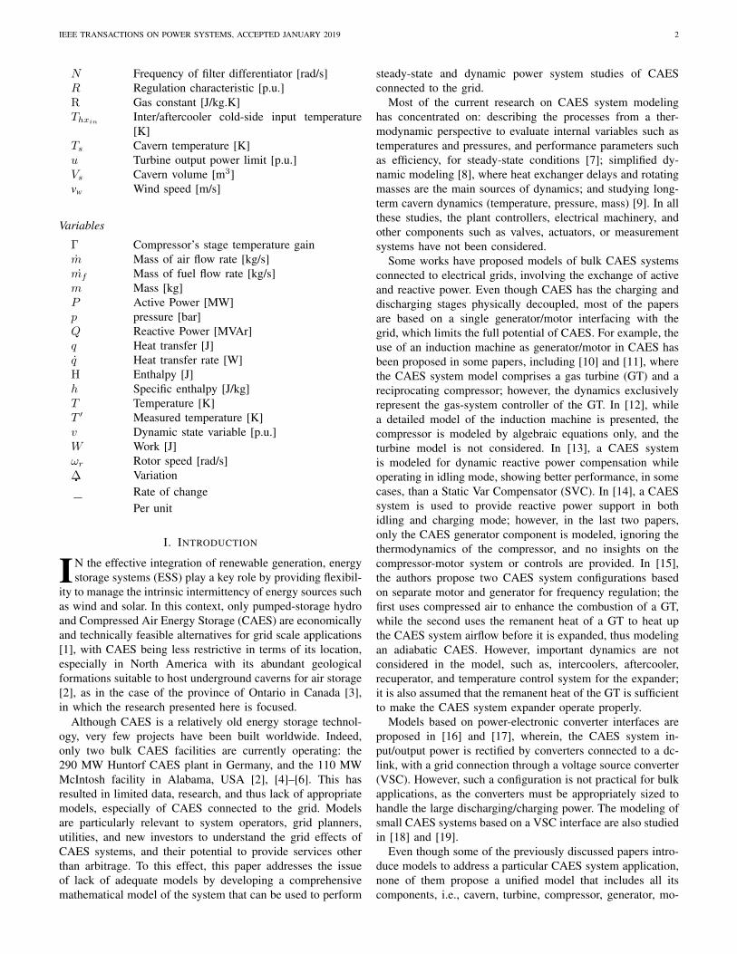
In charging mode, a CAES compressor driven by an elec-trical motor pressurizes the air at ambient conditions, whichis carried through pipes, cooled down in intercoolers and anaftercooler, and stored in the cavern [2]. As the air is injected,the internal pressure of the reservoir and its potential energyincreases. In diabatic CAES systems, in discharging mode, thestored air is preheated in the recuperator, and is then combinedwith gas in the burner before being expanded; on the otherhand, in adiabatic CAES systems, no gas is used, and theair is heated from a heat storage subsystem. The synchronousgenerator’s rotor is moved by the expander to produce electric-ity. In idling mode [21], the CAES system is neither chargingnor discharging. Fig. 1 depicts the following main componentsand interrelations of the underground diabatic CAES facility,based on [5] and [6].• Motor/Generator: A single synchronous or induction

generator/motor can be used in a CAES system. In thispaper, however, the CAES system is modeled using twosynchronous machines, operated and controlled indepen-dently, as in [20].

• Compressor: The compression train comprises a low-pressure axial compressor and a high-pressure multi-stagecentrifugal compressor, to achieve the desired range ofoperating pressures in the cavern. A regulating valve isinstalled after the compression to throttle the compressionpressure down to actual cavern pressure. Intercoolers andan aftercooler are designed to reduce the inlet temperatureat the different compression stages and the air to cavern,to approximate isothermal compression and thus reduce

the power required from the motor [22], reducing lossesand thermal stress on the cavern. In Huntorf, threeintercoolers and one aftercooler are used, and the samehas been modeled here.

• Turbine: In diabatic CAES systems, the turbine has twomain components: the combustion chamber (or burner)and the expander. The air from the cavern is preheated inthe recuperator using the remanent heat of the air leavingthe low-pressure exhaust in the expander, to increaseefficiency [23]. It is then combined with fuel and burnedin the high-pressure combustion chamber to achieve thedesired inlet temperature to the high-pressure expander.After, the air is reheated in a low-pressure burner andexpanded in the low-pressure expander; the reheatingincreases the efficiency of the expansion cycle, as theexpansion work is proportional to the inlet temperaturein a turbine. The turbine can operate in two modes:constant input pressure and variable input pressure [7].In the former, the air is throttled so that the burnerinlet pressure remains constant regardless of the cavernpressure, while in the latter, the burner inlet pressure isthe cavern pressure.

• Cavern: Salt caverns are among the most convenientgeological formations used as reservoirs for undergroundCAES, because of their relatively low overall cost [4], andleak-proof characteristics [24]. The capacity of energystorage depends on the size of the cavern, which is inde-pendent of the size of the turbo machinery. Consequently,the energy-to-power ratio of a CAES system is moreflexible than other storage technologies.

• Control System: The air mass flow in the expansion stageis controlled to realize the desired output power, whilethe inlet temperature in the expanders (low and highpressure) are kept constant by controlling the fuel in theburners (two control loops). The compression air flowrate is regulated by moving the compressor’s variableinlet guide vanes (IGVs), to control power. Consumptionof the motor within a load range of 65 to 110% ofthe rated power [20], which may vary depending on themanufacturer.

III. CAES SYSTEM MODELING

In this section, a comprehensive model of a CAES systemsuitable for power system studies considering two independentsynchronous machines (motor and generator) is proposed,based on [6] and [20]. First, a detailed CAES model whichincludes all the components depicted in Fig. 1 is presented;then, a simplified model is proposed, which would facilitateits implementation in common power system packages fordynamic simulations, without significantly compromising itsaccuracy. Most of the variables defined in the Nomenclaturesection are expressed in per-unit; therefore, if the actualquantities are required, the per-unit values are multiplied bytheir corresponding bases. The proposed models are based onthe following general assumptions [25]:• The proportion of gas to air in the expander is very small,

i.e., mt + mf ≈ mt.


Electrical grid

Cavern Storage

air

air

M G

Charging stage:

1. Synchronous motor

2. LP Compressor

3. HP Compressors

4. Intercoolers

5. Aftercooler

6. Valve

11

Discharging stage:

7. Valve

8. Recuperator

9. High pressure burner

10. High pressure expander

11. Low pressure burner

12. Low pressure expander

13. Synchronous generator

33

44

55

66 77

22

88

99

1010

1111

1212

1313

Electrical grid

Cavern Storage

air

air

M G

Charging stage:


2. LP Compressor

3. HP Compressors

4. Intercoolers

5. Aftercooler

6. Valve

1

Discharging stage:

7. Valve

8. Recuperator

9. High pressure burner

10. High pressure expander

11. Low pressure burner

12. Low pressure expander


3

4

5

6 7

2

8

9

10

11

12

13

, , ,s s s sp V m T

1incT

2incT

inhxT

3incT4incT

1outcT2outcT

4outcT

3outcT

insTsT

e emot motP jQ+

mcP

e eg gP jQ+

mtP

LPxT

bT

HPdTHPxT

LPdT

fmfmgas gas

cm tm

Fig. 1. Configuration of a diabatic, two-machine CAES system based on [6]. All variables are defined in the Nomenclature.

• The air behaves as an ideal gas, i.e., ∆h = cp∆T forexpansion and compression.

• The turbine, compressor, recuperator, intercoolers andaftercooler, and cavern are represented by steady-flowprocesses, i.e., the fluid flows steadily through the controlvolume.

• Changes in kinetic and potential energy in the processesare negligible, i.e., q −W = ∆H.

The detailed model is described in the following two subsec-tions III-A and III-B, and the simplified model in SubsectionIII-C. The cavern model is common for both models and ispresented in Subsection III-D.

A. Discharging ModeThe components involved in the discharging mode are

the recuperator, combustion chambers, expanders, and syn-chronous generator which are described next.

1) Recuperator: The recuperator is modeled as a counter-flow heat exchanger. Its hot side is fed by the exhaust gasesat temperature of the low-pressure turbine TxLP , while the aircoming from the cavern enters the cold side at temperatureTs, reaching Tb at its outlet. Given that the outlet temperatureof the recuperator is unknown, the heat exchanging processcan be described by its effectiveness εr, defined as the ratioof the actual regenerated heat transfer rate over the maximumpossible heat transfer rate as follows [26]:

εr =q

qmax=

hb − hshxLP − hs

(1)

In this case, the maximum possible heat rate exchange ratiooccurs between the inlet of the hot side and inlet of the coldside of the recuperator. It is assumed that the turbine airflowpasses through both sides of the heat exchanger at the sametime, i.e., input flow at hot and cold sides are the same.

From (1), acknowledging that Tb does not change instantlyas heat transfer is a dynamic process, which could be approx-imated by a first order system [27], the input temperature ofthe air to the high-pressure burner T b can be calculated asfollows:

T b =TsTbo

+ vr (2)

vr =1

τR

[εr

(T xLP TxLPo − Ts

Tbo

)− vr

](3)

where vr represents the heat dynamics added by the recuper-ator; Tbo can be found by solving (2) and (3) for steady-stateconditions, and T b = 1 and T xLP = 1.

2) Combustion Chambers or Burners: The combustion inthe burners is produced by a mixture of fuel (gas) andair. In the high-pressure and low-pressure burners, the inlettemperature to their respective expanders TdHP and TdLPrises as the amount of fuel injected into the burners increases(mass flow rate of fuel mf ), and cools down as mt increases.In this paper, it is assumed that the fuel flow in the twoburners are controlled by the same controller; hence, these varyproportionally, i.e., mfHP = mfLP = mf . From the energybalance of the combustion chamber, and assuming isobaric


heat addition, the inlet temperature of the high-pressure andlow-pressure expanders, in p.u. of their nominal values, canbe obtained as follows [28]:

T dHP = T b

(TboTdHPo

)+TdHPo − Tbo

TdHPo

(mf

mt

)(4)

T dLP = T xHP

(TxHPoTdLPo

)+TdLPo − TxHPo

TdLPo

(mf

mt

)(5)

where the inlet temperature of the air at the high-pressureburner is Tb, while the inlet temperature at the low-pressureburner is equal to the exhaust temperature of the high-pressureturbine TxHP .

3) Expander: For an isentropic air expansion at each stage,the corresponding isentropic exhaust temperatures Txik be-comes a function of the turbine’s stage pressure ratio πtk andinlet temperature as follows [7]:

TxikTdk

= π− γ−1

γ

tk(6)

where γ = cp/cv is the heat capacity ratio, and k ={LP,HP}. However, the actual turbine deviates from the isen-tropic idealization, which can be accounted by the isentropicefficiency ηtik as follows [25]:

ηtik∼=

hdk − hxkhdk − hxik

(7)

From (6) and (7), and assuming that the actual pressure ratioof a turbine is approximately equal to its nominal value timesthe air flow rate in p.u. [28]–[30], the exhaust temperature ofthe high-pressure and low-pressure expanders in p.u. can becalculated as follows:

T xk =TdkoT dk

Txko

1−

1− 1(πtkomt

) γ−1γ

ηtik (8)

For a steady-flow, the rate of change of the internal energyof a turbine is zero; hence, the total mechanical power deliv-ered to the generator shaft can be computed as the summationof the difference in rate of change of enthalpy between theinlet and outlet of each expansion stage, as follows:

Ptm =∑k

Ptmk =∑k

(Hdk − Hxk

)(9)

If the enthalpy is expressed as the specific enthalpy times themass, then the turbine’s mechanical power becomes a functionof the rate of change of the mass and the temperature differ-ence between the turbine’s inlet and outlet. Hence, assumingfriction losses represented by the mechanical efficiency ηtmk ,the output mechanical power of each expansion stage, in p.u.ofthe total nominal turbine power, can be approximated by:

P tmk =

(ηtkmcpmto

103Ptmo

)mt

(TdkoT dk − TxkoT xk

)(10)

where Tdok and Ptmo are turbine’s parameters; Txko can befound by solving (8) for T dk = 1, T xk = 1, and mt = 1; andmto can be found by solving (9) and (10) for Ptm = Ptmo .

4) Synchronous Generator: The synchronous generatormodel is well-defined in the literature. One of the mostcommonly used models for dynamic studies is the classicalsubtransient model, which is described in detail in [31].

5) Control System: The control system proposed for theexpansion stage is shown in Fig. 2, and is based on the modelspresented in [28], [30], and [32] for traditional GTs. Thiscontrol considers a speed controller (governor) and a low-pressure exhaust temperature controller. The governor uses

Fuel

flo

w s

yst

em

Turbine equations

x

1c

2c

Recuperator

Synchronous

generator

Air flow system

Power transducer

Temperature measurement system

Governor

sT

LPxT

reftP

+

1

R

LPxT

bT

'

LPxT

+

+ +

+

+

1

i

p

t

t

KK

s

maxu

minu

1

1 TDs

1

1 AVs

maxg

ming

tm

1

1 TPs

mtP

+

egP

1

2 t tH s Dtr

fm

1

1 SFs

1

1 Ss

refxT

i

p

T

T

KK

s

4

1

1 s

5

4

31

KK

s

max

F min

F

Fig. 2. Control system for CAES expansion stage.

the speed deviation signal ∆ωrt in a negative feedback loopto modify the power reference P tref (set manually or byan external AGC signal) creating a steady-state error in thespeed, according to the proportional gain 1/R (regulationcharacteristic). The modified power reference is comparedwith a measured mechanical output power using a powertransducer, and the error is passed through a PI controller(governor) which can be tuned to provide good tracking errorwhile achieving a desired dynamic response. The output ofthe governor is fed into the air flow system, which is modeledby two first-order transfer functions, with time constants τTD

and τAV representing the turbine’s discharge delay, and thevalve air opening system including its limits, correspondingly.

The fuel control branch compares the measured low-pressure exhaust temperature signal T

′xLP to a reference

temperature T xref , and the error is processed by another PIcompensator that controls the fuel system. The temperaturemeasurement system comprises a thermocouple and a radiationshield. The output signal of the PI controller is multiplied bythe p.u. rotor speed before being sent to the fuel system, asthe operation of the latter depends on the speed, since it isattached to the rotor shaft as indicated in [30]. This signal is


then multiplied by the gain c1 and added to the constant c2,which represents the fuel consumption at no load in p.u.; c1compensates for the offset introduced by c2, and c1 + c2 = 1.

There are two delays associated with the fuel system, onefor the valve positioning system that controls the amount offuel injected, and the other for the downstream piping andgas distribution manifold, both modeled as first order transferfunctions connected in series when the fuel is a gas [32]. Theoutput of the fuel flow system is mf , and the flow rates mt andmf , and T b are inputs to the burners and expanders modeledusing (2), (3), (4), (5), (8)-(10). Voltage control is provided bythe excitation system of the synchronous generator.

B. Charging Mode

The components involved in this operational mode are thecompressor, intercoolers, aftercooler, and synchronous motor.The model presented next allows frequency regulation by thecompressor. The high-pressure compressor is modeled as amulti-stage compression system with an intercooler betweeneach stage, while the low-pressure compression is modeled asa single stage compression [22]; an intercooler is also usedbetween the low- and high-pressure compressors. The index jis used to identify the different compression stages as follows:j = 1 for low-pressure stage; j = 2 for high-pressure firststage; j = 3 for high-pressure second stage; and j = 4 forhigh-pressure third stage.

1) Compressor plus heat exchanger: Using similar expres-sions as those presented for the turbine, a compression stagecan be modeled as a temperature gain Γj(mc) plus a heatexchanger, as depicted in Fig. 3, where:

xx

++ +

in jcT out j

cT

( )j cm

cm

+

+

+

inhxT

1

j

j

hx

hxs

+

j

1in jcT

+

cm

m jcP

mcP

Fig. 3. Model of one compression stage with a heat exchanger at the output.

Γj(mc) = 1 +

[πcj (mc)

] γ−1γ − 1

ηcij(11)

Φj =cpmco

103ηcmjPcmo

(12)

The pressure ratio of each compression stage πcj is afunction of the air flow, as determined by a compressor map;here, the compressor map is modeled using the equation of anellipse, as suggested in [33]. Hence, the pressure ratio of eachcompressor stage can be calculated as follows:

πcj (mc) = a1j

√1− mc

a2j(13)

πcj (mco) = πcjo (14)

πcj (0.5mco) = 1.12πcjo (15)

Equations (14)-(15) represent two operating points in thecompressor map, and are used to find its parameters a1j anda2j . In Fig. 3, P cmj is the mechanical power consumed bythe compressor at the stage j in p.u. of the total nominalcompressor power, and P cm is the total mechanical powerconsumed by the compressor in p.u.; Tcinj and Tcoutj arethe inlet and outlet temperatures of a compressor stage re-spectively. The heat exchangers of stages j = 1, 2, 3 representintercoolers, and are modeled with effectiveness εhxj and timeconstant τhxj . The inlet temperature at the cold side of all heatexchangers Thxin is the same, and remains constant assumingthat the heat capacity rate of the cooling fluid (water) is muchhigher than the compressor air flow’s heat capacity rate. Theaftercooler corresponds to the heat exchanger of stage j = 4.

2) Synchronous Motor: The synchronous motor is mod-eled using the same subtransient model as the synchronousgenerator [31], with the motor driving the mechanical load(compressor).

3) Control System: As illustrated in Fig. 4, the mechanicalpower required by the compressor depends on the air flowrate, which is controlled by moving the variable inlet guidevanes. A feedback of the rotor’s speed deviation modifies thereference power P cref , as in the generator case; however,the sign of this feedback is positive in the governor loop,because the compressor has to decrease its power consumptionwhen the frequency drops, and do the opposite when thefrequency increases. The error between the measured powerand the modified reference power is passed through a PIDgovernor which sends the signal to the IGVs, whose operationis assumed to be linear with respect to mc.

The air flow dynamics due to mass flow accumulation ateach compression stage are very fast, hence, their combinedeffect is modeled by a single transfer function with timeconstant τCD [32]. The output of this series arrangement oftransfer functions is multiplied by the rotor speed to obtainmc, since the actual air flow depends on the rotational speed ofthe compressor. Unlike the turbine, the discharge temperatureof the compressor is not controlled, and lmin and lmax

are limits in the air flow to prevent the compressor fromoperating in surge or choke conditions (usually 60% to 100%of the nominal air flow). Finally, mc is used as input to thecompressor stages, as shown in Fig. 3. The voltage control isprovided using the same model as for the generator.


Dynamic

compressor model

1

Power transducer

+

+

Synchronous

motor

+

+

+

Governor

+

i d

p

c c

c

K sKK

s N s

refcP

1

1 IGVs

maxl

minl

cr

cm

inhxT

1incT insT

mcP

1

1 CDs

emotP

1

2 c cH s D

1

1 CPs

cr

1

R

Fig. 4. Control system for CAES compression stage.

C. Simplified Model of CAES System

1) Expansion: As is typically done in gas turbines tosimplify their mechanical model, the HP and LP expansionstages can be approximated by a single stage [33]. Thus,assuming that the low-pressure and high-pressure expansionstages have the same pressure ratio, and adding the reheatingeffect of the low-pressure burner, the CAES turbine exhausttemperature can be calculated as follows:

T x =TdoT d + ∆To

(mf

mt

)Txo

1−

1− 1(πtomt

) γ−12γ

ηti

(16)

where πto = πtLPoπtHPo is the total expansion pressureratio. The term ∆To

(mf

mt

)represents the inlet low-pressure

temperature rise due to the low-pressure burner. The totalmechanical output power can then be calculated as follows:

P tm =ηtiηtmcpmt

(2Td + ∆To

(mf

mt

))103Ptmo

1− 1(πtomt

) γ−12γ

(17)

where ηti and ηtm are the equivalent mechanical and isentropicefficiency of the expansion correspondingly. The recuperator,high-pressure burner (now referred to as burner), and controlsystem remain the same as in the detailed model, substitutingTx for TxLP , and Td for TdHP .

2) Compression: The high-pressure multi-stage compressorcan be reduced to a single-stage compressor, assuming idealoperation of the intercoolers, which would keep the inlettemperature of each stage equal to the inlet condition ofthe first high-pressure stage (isothermal compression) [34].Under these assumptions, the CAES compressor could bemodeled using two stages of the compression-heat-exchangerillustrated in Fig. 3, with j = 1 representing the low-pressurecompressor, and j = 2 the high-pressure compressor. Hence,

the temperature gain Γ2(mc) and compressor’s stage powerconstant Φ2 become:

Γ2(mc) = 1 +

[πc2(mc)

] γ−13γ − 1

ηci2(18)

Φ2 =3cpmco

103ηcm2Pcmo

(19)

to account for the reduction of the three compressor stages.In this case, πc2 is the total pressure ratio of the high-pressure compressor, ηcm2

is the total mechanical efficiency,and ηci2 is the equivalent isentropic efficiency of the singlestage high-pressure compressor. The heat-exchanger for stagej = 2 represents the aftercooler in this model, whereasthe low-pressure compressor (j = 1), electrical motor, andcontrol system remain the same as in the detailed model. Theequivalent simplified CAES facility is shown in Fig. 5.

Electrical grid

Cavern Storage

air

air

M G

Charging stage:


2. LP Compressor

3. HP Compressor

4. Intercooler

5. Aftercooler

6. Valve

11

Discharging stage:

7. Valve

8. Recuperator

9. Burner

10. Expander


33

44

55

66 77

22

88

99

1010

1111

gas

cm tm

1incT

1outcT

inhxT

2incT

mcP

2outcT

insTinsT

, , ,s s s sp V m T

bT

e emot motP jQ+e eg gP jQ+

mtP

dT

fmfm

Fig. 5. Simplified CAES model.

D. Cavern Model

From the conservation of mass in an open system consid-ering the cavern as a control volume, the mass in p.u. can becalculated as follows:

ms =1

mso

(mcmco − mtmto

)(20)

mso =105psoVs

RTs(21)

From the conservation of energy and the state equation definedby the Ideal Gas Law, the pressure for an adiabatic andisochoric cavern can be calculated as follows [9]:

ps =Rγ

105 Vs pso

(mcmcoT sinTsino − mtmtoTs

)(22)


Since the proposed dynamic model is developed to studythe CAES system for about 200 s, it is assumed here that theinternal temperature of the cavern Ts remains constant duringthe period of analysis. In these equations, the pressure andmass are expressed in p.u. of the cavern’s nominal values.The initial conditions for the integration of ms and ps aremsref and psref , respectively.

IV. RESULTS AND DISCUSSION

In this section, step changes in the reference values are firstsimulated, with results being compared to the models proposedin [15] and [16]. Since the proposed CAES system model ishighly nonlinear and comprises several dynamic sub-systemsand controls, such as temperature control, heat exchangers,measurement systems, etc., step-changes are used to studythe controls and system dynamic responses without externaldisturbances, and to highlight the differences with respectto existing models. Then, operation of the proposed CAESsystem models is compared with a traditional GT model andthe simplified model in [15] to provide frequency regulationfor a grid with high penetration of wind generation. Parametersof the CAES Huntorf plant available from [6], [22], [35], [36]and [37] were used in the presented simulations; the corre-sponding dynamic data was taken from [27], [30], [32], [35],and [38], and the turbomachinery inertias were obtained from[39]. The isentropic efficiencies of the expansion stages andhigh-pressure compression stage were calculated for nominalturbine and compressor conditions. The gains of the PI andPID controllers were obtained by trial and error to producethe best possible dynamic response of the CAES system. Allparameters used in the simulations are shown in Table I.

A. Dynamic Performance Studies

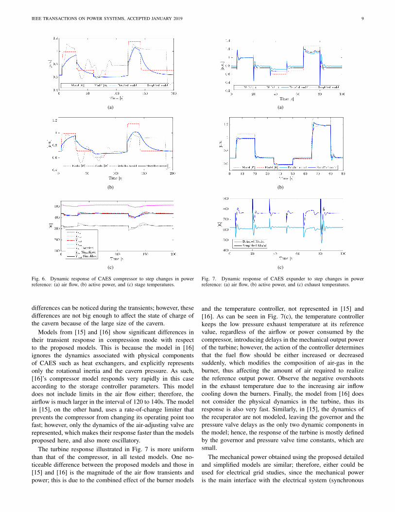
A 280 MW turbine and 60 MW compressor supply-ing/consuming 0.7 p.u. power, respectively, were simulated inMatlab/Simulink. Step changes of +0.3, -0.3, -0.1, +0.1, +0.5,and -0.5 p.u. were respectively applied at t = 5s, 20s, 35s, 50s,65s, and 80s in the turbine power reference; and at t = 5s, 30s,60s, 80s, 120s, and 140s in the compressor power referenceof both the proposed models, detailed and simplified. In bothcases, the speed deviation feedback with the permanent droopcharacteristic R is disconnected. The response of these modelsis also compared with two existing CAES models describedin [15] and [16], with the primary-frequency control feedbackdisabled in [15], and not considering the converters interfacingthe grid in [16], but representing the storage controller with themechanical power generated/consumed by the CAES systemas its input signal; the PI controller parameters of the latterwere also tuned to obtain the best dynamic performance. Thedynamic response of the compression and expansion stagesare shown in Fig. 6 and Fig. 7, respectively.

In Fig. 6, observe that, even though the simplified modelconsiders only the dynamics of one intercooler, it has avery similar response to the detailed model. This is due tothree factors. First, the airflow is almost equal at each stageof compression, as discussed in Section III-B3. Second, theoutput temperature of the intercooler at stage j+ 1 is directly

TABLE ICAES AND SYSTEM PARAMETERS

Discharging modeParameter Value Parameter Value Parameter ValueTdHPo [K] 823.15 TdLPo [K] 1098.2 TxHPo [K] 612.15TxLPo [K] 668.15 πtHPo 3.818 πtLPo 10.856ηtHPm [p.u.] 0.99 ηtLPm [p.u.] 0.99 ηtHPi [p.u.] 0.8065ηtLPi [p.u.] 0.7926 Tbo [K] 599.15 εr[p.u.] 0.80cp[kJ/kg.K] 1.055 Ptmo [MW ] 280 γ 1.4mto [kg/s] 417 mfo [kg/s] 12 τR[s] 25K4 0.8 K5 0.2 τ3[s] 15τ4[s] 2.5 KTp 7 KTi 5τS [s] 0.05 τSF [s] 0.4 Fmax[p.u.] 1.25Fmin[p.u.] 0 c2[p.u.] 0.05 τAV [s] 0.1τTD[s] 0.3 gmax[p.u.] 1.25 gmin[p.u.] 0.1R[p.u.] 0.04 Ktp 3 Kti 2τTP [s] 0.02 umax[p.u.] 1.2 umin[p.u.] 0Ht[s] 3.9821 Dt[p.u] 2 KAGC2 [p.u.] 60

Discharging mode simplified modelParameter Value Parameter Value Parameter Value∆To[K] 315.73 Txo [K] 762.41 ηti [p.u.] 0.7995ηtm [p.u.] 0.9801 πto 41.451

Charging modeParameter Value Parameter Value Parameter ValueTcin1 [K] 283.15 Tcout1o [K] 497.6 εhx1

0.8785Tcin2o [K] 323.15 Tcout2o [K] 420.5 εhx2



0.8ηci1 [p.u.] 0.8200 ηcm1 [p.u.] 0.99 πc1o 5.4290ηci2 [p.u.] 0.9115 ηcm2 [p.u.] 0.99 πc2o 2.3460ηci3 [p.u.] 0.9023 ηcm3 [p.u.] 0.99 πc3o 2.3460ηci4 [p.u.] 0.9097 ηcm4 [p.u.] 0.99 πc4o 2.3460τhx1

[s] 12 τhx2[s] 12 τhx3

[s] 12τhx4

[s] 12 Hc[s] 12.957 Dc[p.u.] 0Pcmo [MW ] 58.7 γ 1.4 cp[kJ/kg.K] 1.055Thxin [K] 298.7 R[p.u.] 0.04 Kcd 0.214Kcp 0.4147 Kci 0.1485 N [rad/s] 1.0792τCD[s] 0.2 τIGV [s] 0.2 lmax[p.u.] 1.15lmin[p.u.] 0.6 τDr[s] 1.5 τCP [s] 0.02Kdroop[p.u.] 2000 mco [kg/s] 108

Charging mode simplified modelParameter Value Parameter Value Parameter Valueπc2o 12.9117 ηci2 [p.u.] 0.9142 ηcm2 [p.u.] 0.9703

CavernParameter Value Parameter Value Parameter Valuepso [bar] 42 Vs[m3] 300000 Ts[K] 323.15R[J/kg.K] 287.058

SystemParameter Value Parameter Value Parameter ValuePGTo[MW ] 213.4 PST1o[MW ] 200 PST2o[MW ] 200Pwo[MW ] 200 HGT [s] 18.5 HST1[s] 3.17HST2[s] 3.17 Hw[s] 3 KAGC1 [p.u.] 20

affected by the instantaneous change of the output temperatureof the previous stage j, which is then modified slowly as theheat is removed. Finally, each compression stage contributesto the total consumed power independently, as shown in Fig. 3.Notice that for every step change there is a fast transient in theproposed models produced by the rapid change in the air flow,and the initial response of the intercoolers. At time t = 130s,the air flow reaches its maximum limit; however, a droppingairflow is observed because the actual air flowing through thecompressor is a function of the rotor speed, as shown in Fig. 4.Observe that no control action was taken on the compressor’sdischarge temperature; hence, the temperatures at the differentstages present similar transients as mc, as shown in Fig. 6(c).The input temperatures to the cavern Tsin in the detailed andsimplified models are similar in steady-stage, although some


(a)

(b)

(c)

Fig. 6. Dynamic response of CAES compressor to step changes in powerreference: (a) air flow, (b) active power, and (c) stage temperatures.

differences can be noticed during the transients; however, thesedifferences are not big enough to affect the state of charge ofthe cavern because of the large size of the cavern.

Models from [15] and [16] show significant differences intheir transient response in compression mode with respectto the proposed models. This is because the model in [16]ignores the dynamics associated with physical componentsof CAES such as heat exchangers, and explicitly representsonly the rotational inertia and the cavern pressure. As such,[16]’s compressor model responds very rapidly in this caseaccording to the storage controller parameters. This modeldoes not include limits in the air flow either; therefore, theairflow is much larger in the interval of 120 to 140s. The modelin [15], on the other hand, uses a rate-of-change limiter thatprevents the compressor from changing its operating point toofast; however, only the dynamics of the air-adjusting valve arerepresented, which makes their response faster than the modelsproposed here, and also more oscillatory.

The turbine response illustrated in Fig. 7 is more uniformthan that of the compressor, in all tested models. One no-ticeable difference between the proposed models and those in[15] and [16] is the magnitude of the air flow transients andpower; this is due to the combined effect of the burner models

(a)

(b)

(c)

Fig. 7. Dynamic response of CAES expander to step changes in powerreference: (a) air flow, (b) active power, and (c) exhaust temperatures.

and the temperature controller, not represented in [15] and[16]. As can be seen in Fig. 7(c), the temperature controllerkeeps the low pressure exhaust temperature at its referencevalue, regardless of the airflow or power consumed by thecompressor, introducing delays in the mechanical output powerof the turbine; however, the action of the controller determinesthat the fuel flow should be either increased or decreasedsuddenly, which modifies the composition of air-gas in theburner, thus affecting the amount of air required to realizethe reference output power. Observe the negative overshootsin the exhaust temperature due to the increasing air inflowcooling down the burners. Finally, the model from [16] doesnot consider the physical dynamics in the turbine, thus itsresponse is also very fast. Similarly, in [15], the dynamics ofthe recuperator are not modeled, leaving the governor and thepressure valve delays as the only two dynamic components inthe model; hence, the response of the turbine is mostly definedby the governor and pressure valve time constants, which aresmall.

The mechanical power obtained using the proposed detailedand simplified models are similar; therefore, either could beused for electrical grid studies, since the mechanical poweris the main interface with the electrical system (synchronous


generator). Only the magnitude of the transients presentssome differences between these models; however, the steady-state magnitudes of the airflow and temperature present somedifferences due to the assumption of equal pressure ratios inthe high and low-pressure expanders.

Note that a clear advantage of the simplified model is areduction in the amount and detail of the parameters required.Thus, in the detailed model, the input and output temper-atures, efficiency, effectiveness and time constants of heatexchangers, pressure ratios, etc., must be specified for eachcompression/expansion stage. The required information maybe unavailable or may require extensive machine testing andmeasurements. Estimating these parameters is complicated dueto the interrelations between variables within the differentstages; furthermore, initializing the model is cumbersome. Onthe other hand, the proposed simplified CAES model involvesfewer parameters because of the lumped representation usedin this model, such as the nominal pressure ratio of the HPcompressor or the inlet temperature of the turbine. Moreover,the complexity of the parameter estimation is reduced asseveral internal variable relations are avoided.

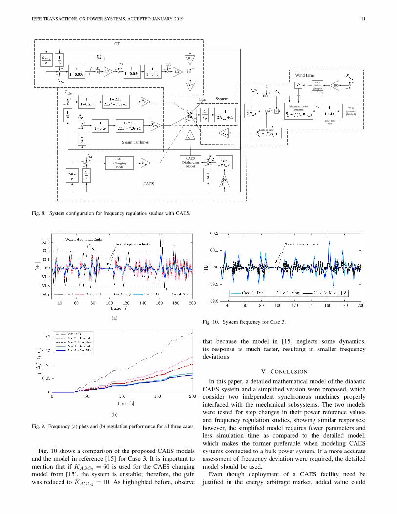
B. Frequency Regulation

The power system model shown in Fig. 8 is used to study theimpact of CAES in frequency regulation; the electrical systemis approximated by transfer functions, since the system dy-namic responses are much faster than the mechanical systemswhich are represented in some detail in the model and moresignificantly impact the system’s frequency response. The testsystem comprises relevant and realistic models of differentgeneration technologies, and configuring the system to have33% of the load being supplied by wind generation, whichis the main source of frequency disturbance. Steam and gasgenerators were sized to be able to supply the demand evenwhen the wind power goes to zero, with corresponding realisticdynamic data. The base case (Case 1) comprises a fixed loadof 650 MW, a 200 MW wind farm, two 200 MW steamturbine units contributing to primary frequency regulation,and a 213.4 MW gas turbine (GT) that provides primaryand secondary frequency regulation. Secondary control isadded by integrating the speed deviation, which emulates atraditional Automatic Generation Control (AGC). In Case 2,one steam turbine units is replaced by a 280 MW-discharging/60 MW-charging CAES system, which operates in dischargingmode only. Finally, in Case 3, the CAES system operates insimultaneous charging and discharging modes.

The initial conditions for the three cases are summarizedin Table II. The system is in steady-state at 60 Hz nominalfrequency before t = 30 s. The gains KAGC1

= 20, andKAGC2

= 60 for the GT and CAES turbine, respectively, weretuned to achieve the best frequency performance; furthermore,in order to improve the response of the compressor, a transientdroop control was added, as shown in Fig. 8. The wind farm iscomprised of a simple aggregation of 100 2-MW Doubly-FedInduction Generators (DFIG), based on the models reportedin [40] and [41]. The wind profile was artificially createdusing a Weibull distribution (shape parameter k=2, and scale

TABLE IIINITIAL CONDITIONS FOR SIMULATED CASES

Case 1 Case 2 Case 3Steam generation [MW] 350 175 175Wind generation [MW] 200 200 200GT generation [MW] 100 100 100CAES generation [MW] - 175 221.96CAES compressor load [MW] - - 46.96

parameter Λ = 12.1505), which was smoothed out with a low-pass filter [42]. The steam turbine model and parameters weretaken from [31]. The model proposed in [32] was used for theGT, excluding the acceleration control and assuming the useof gas as fuel.

A comparison of the system frequency for Cases 1, 2, and3 for the proposed detailed and simplified CAES models arepresented in Fig. 9 (a). The normal and abnormal operationlimits are as per the Ontario’s Independent Electricity SystemOperator (IESO) [43]. The results show very similar frequencyresponses for the simplified and detailed CAES models inCases 2 and 3; the main difference is the magnitude of thefrequency excursions, which, as discussed in Section IV-A,are better captured by the detailed model. The largest error inthe frequency deviation between the simplified and detailedmodels is 0.03 Hz (0.05%). The simplified model had theadditional advantage of requiring less than half as much timeto simulate as did the corresponding more detailed model(17.8s vs. 38.8s for Case 3). Observe that the combinedoperation of compressor and turbine in Case 3 produces abetter frequency regulation than Cases 1 and 2. Thus, themaximum positive frequency excursion is reduced from 60.39Hz in Case 1, to 60.17 Hz in Case 2, and 60.16 Hz inCase 3; and the largest negative frequency excursion decreasesfrom 59.68 Hz, to 59.89 Hz, and 59.89 Hz, respectively.Furthermore, for the considered simulation period, in Case3 the combined charging and discharging is more effectivein flattening out the frequency than in the other two cases;this can be attributed to the operation of the compressor usingthe proposed transient droop control, and the inertia added bythe rotating masses of the compressor and synchronous motor.Similarly, the number of frequency excursions beyond limitsis reduced from 5 to 0 when comparing Case 1 to Cases 2 or3.

In Fig. 9 (b), the cumulative absolute value of frequencydeviation is used as a quantitative measurement of the perfor-mance of each alternative considered. Note that the detailedmodel yields a larger cumulative frequency deviation than thereduced model in both Cases 2 and 3; thus, the differencebetween the two models for Case 2 is around 20%, while itis 10% for Case 3. Nevertheless, from this metric, it can beconcluded that Case 2 is better than Case 1, and Case 3 isbetter than the other two. At the end of the simulation time,comparing the results of the detailed models, the value forCase 2 is 58.89% of that in Case 1, and 31.98% for Case 3with respect to Case 1. A quasi-linear trend is observed inthe three plots; thus, the relative proportion of this metric isexpected to remain constant in time.


Wind

generator

(Weibull)

Look-up table

1

+ +

300+

+/

Mechanical power

extracted

Rate

limiter

(3deg/s)

0

Low-pass

filter

+x

1

0.7

0.23

+ +

0.5

1.3

0.23+

+

+ + +

+

+ Load

CAES

Charging

Model

CAES

Discharging

Model

+

++

++

+

+

+

+

GT

Steam Turbines

CAES

System

Wind farm

Fig. 8. System configuration for frequency regulation studies with CAES.

(a)

(b)

Fig. 9. Frequency (a) plots and (b) regulation performance for all three cases.

Fig. 10 shows a comparison of the proposed CAES modelsand the model in reference [15] for Case 3. It is important tomention that if KAGC2 = 60 is used for the CAES chargingmodel from [15], the system is unstable; therefore, the gainwas reduced to KAGC2

= 10. As highlighted before, observe

Fig. 10. System frequency for Case 3.

that because the model in [15] neglects some dynamics,its response is much faster, resulting in smaller frequencydeviations.

V. CONCLUSION

In this paper, a detailed mathematical model of the diabaticCAES system and a simplified version were proposed, whichconsider two independent synchronous machines properlyinterfaced with the mechanical subsystems. The two modelswere tested for step changes in their power reference valuesand frequency regulation studies, showing similar responses;however, the simplified model requires fewer parameters andless simulation time as compared to the detailed model,which makes the former preferable when modeling CAESsystems connected to a bulk power system. If a more accurateassessment of frequency deviation were required, the detailedmodel should be used.

Even though deployment of a CAES facility need bejustified in the energy arbitrage market, added value could


be obtained in other markets, such as the ancillary servicemarket. In particular, it was demonstrated in this paper that aCAES connected to a power system could provide frequencyregulation, operating in simultaneous charging and dischargingmodes, contributing to significantly reduce the cumulativefrequency deviation of the system. This is only possible in aconfiguration with independent generator and motor machines,as proposed here. Future work includes implementing andtesting the proposed models in a benchmark power systemfor realistic transient and frequency stability studies.

REFERENCES

[1] B. Cleary, A. Duffy, A. O’Connor, M. Conlon, and V. Fthenakis,“Assessing the economic benefits of compressed air energy storage formitigating wind curtailment,” IEEE Trans. Sustain. Energy, vol. 6, no. 3,pp. 1021–1028, 2015.

[2] “EPRI-DOE handbook of energy storage for transmission & distributionapplications,” Tech. report, EPRI and U.S. Department of Energy, PaloAlto, CA, and Washington, DC, pp. 3–35, 2003.

[3] J. Konrad, R. Carriveau, M. Davison, F. Simpson, and D. S.-K. Ting,“Geological compressed air energy storage as an enabling technologyfor renewable energy in Ontario, Canada,” Int. J. Environmental Stud.,vol. 69, no. 2, pp. 350–359, 2012.

[4] J. Simmons, A. Barnhart, S. Reynolds, and S. Young-Jun, “Studyof compressed air energy storage with grid and photovoltaicenergy generation,” Tech. report, The Arizona Research Institutefor Solar Energy (AzRISE)-APS, 2010. [Online]. Available: http://u.arizona.edu/$\sim$sreynold/caes.pdf

[5] S. Succar and R. H. Williams, “Compressed air energystorage: theory, resources, and applications for wind power,”Tech. report, Princeton Environmental Institute, 2008. [On-line]. Available: https://acee.princeton.edu/wp\-content/uploads/2016/10/SuccarWilliams\ PEI\ CAES\ 2008April8.pdf

[6] “Huntorf air storage gas turbine power plant,” Tech. report No. DGK 90 202 E, Brown Boveri (BBC), Germany. [Online]. Available:www.solarplan.org/Research/BBC\ Huntorf\ engl.pdf

[7] P. Zhao, L. Gao, J. Wang, and Y. Dai, “Energy efficiency analysis andoff-design analysis of two different discharge modes for compressed airenergy storage system using axial turbines,” Renewable Energy, vol. 85,pp. 1164–1177, 2016.

[8] Y. Mazloum, H. Sayah, and M. Nemer, “Static and dynamic modelingcomparison of an adiabatic compressed air energy storage system,” J.Energy Resources Technol., vol. 138, no. 6, p. 062001, 2016.

[9] W. He, X. Luo, D. Evans, J. Busby, S. Garvey, D. Parkes, andJ. Wang, “Exergy storage of compressed air in cavern and cavern volumeestimation of the large-scale compressed air energy storage system,”Applied Energy, vol. 208, pp. 745–757, 2017.

[10] T. Xia, L. He, N. An, M. Li, and X. Li, “Electromechanical transientmodeling research of energy storage system based on power systemsecurity and stability analysis,” in IEEE Int. Conf. on Power Syst.Technol. (POWERCON), Chengdu, China, 2014, pp. 221–226.

[11] L. He, T. Xia, F. Tian, and N. An, “Modeling and simulation ofcompressed air energy storage (CAES) system for electromechanicaltransient analysis of power system,” Advanced Materials Research, vol.860, pp. 2486–2494, 2014.

[12] M. V. Dahraie, H. Najafi, R. N. Azizkandi, and M. Nezamdoust, “Studyon compressed air energy storage coupled with a wind farm,” in IEEE2nd Iranian Conf. on Renewable Energy and Distributed Generation(ICREDG), Tehran, Iran, 2012, pp. 147–152.

[13] H. T. Le and S. Santoso, “Increasing wind farm transient stabilityby dynamic reactive compensation: Synchronous-machine-based ESSversus SVC,” in IEEE Power and Energy Society General Meeting,Minneapolis, MN, 2010, pp. 1–8.

[14] ——, “Operating compressed-air energy storage as dynamic reactivecompensator for stabilising wind farms under grid fault conditions,” IETRenewable Power Generation, vol. 7, no. 6, pp. 717–726, 2013.

[15] I. Kandiloros and C. Vournas, “Use of air chamber in gas-turbine unitsfor frequency control and energy storage in a system with high windpenetration,” in IEEE PES Innovative Smart Grid Technol. Conf. Europe(ISGT-Europe), Istanbul, Turkey, 2014, pp. 1–6.

[16] A. Ortega and F. Milano, “Generalized model of VSC-based energystorage systems for transient stability analysis,” IEEE Trans. Power Syst.,vol. 31, no. 5, pp. 3369–3380, 2016.

[17] N. Hasan, M. Y. Hassan, M. S. Majid, and H. A. Rahman, “Mathematicalmodel of compressed air energy storage in smoothing 2MW windturbine,” in IEEE Int. Power Eng. and Optimization Conf. (PEDCO),Melaka, Malaysia, 2012, pp. 339–343.

[18] Z. Xiaoshu and Z. Hong, “Switched reluctance motor/generator sim-ulation research based on compressed air energy storage system,” inInt. Conf. on Advanced Mechatronic Syst. (ICAMechS), Beijing, China,2015, pp. 479–484.

[19] M. Martınez, M. Molina, and P. Mercado, “Dynamic performance ofcompressed air energy storage (CAES) plant for applications in powersystems,” in IEEE PES Transmission and Distribution Conf. and Expo.:Latin America (T&D-LA), Sao Paulo, Brazil, 2010, pp. 496–503.

[20] “SMARTCAES Compressed Air Energy Storage Solutions,” Brochure,DRESSER-RAND, 2015. [Online]. Available: www.dresser-rand.com

[21] H. Daneshi, A. Srivastava, and A. Daneshi, “Generation scheduling withintegration of wind power and compressed air energy storage,” in IEEEPES Transmission and Distribution Conf. and Expo., New Orleans, LA,2010, pp. 1–6.

[22] B. J. Davidson, I. Glendenning, R. D. Harman, A. B. Hart, B. J.Maddock, R. D. Moffitt, V. G. Newman, T. F. Smith, P. J. Worthington,and J. K. Wright, “Large-scale electrical energy storage,” IEE Proc. A -Physical Science, Measurement and Instrumentation, Management andEducation - Reviews, vol. 127, no. 6, pp. 345–385, 1980.

[23] R. B. Schainker and M. Nakhamkin, “Compressed-air energy storage(CAES): Overview, performance and cost data for 25MW to 220MWplants,” IEEE Trans. Power App. Syst., no. 4, pp. 790–795, 1985.

[24] K. Allen, “CAES: The underground portion,” IEEE Trans. Power App.Syst., vol. PAS-104, no. 4, pp. 809–812, July 1985.

[25] Y. Cengel and M. Boles, Thermodynamics: An Engineering Approach.8th ed., NY: McGraw-hill, 2002.

[26] T. L. Bergman and F. P. Incropera, Fundamentals of heat and masstransfer. 6th ed., NY: John Wiley & Sons, 2007.

[27] H. A. d. S. Mattos, C. Bringhenti, D. F. Cavalca, O. F. R. Silva, G. B. d.Campos, and J. T. Tomita, “Combined cycle performance evaluation anddynamic response simulation,” Aerosp. Electron. Syst. Mag., vol. 8, no. 4,pp. 491–497, 2016.

[28] IEEE Working Group on Prime Mover and Energy Supply Models forSystem Dynamic Performance Studies, “Dynamic models for combinedcycle plants in power system studies,” IEEE Trans. Power Syst., vol. 9,no. 3, pp. 1698–1708, Aug 1994.

[29] J. Mantzaris and C. Vournas, “Modelling and stability of a single-shaftcombined cycle power plant,” Int. J. Thermodynamics, vol. 10, no. 2,pp. 71–78, 2007.

[30] N. Kakimoto and K. Baba, “Performance of gas turbine-based plantsduring frequency drops,” IEEE Trans. Power Syst., vol. 18, no. 3, pp.1110–1115, 2003.

[31] P. Kundur, Power system stability and control. NY: McGraw-hill, 1994.[32] W. I. Rowen, “Simplified mathematical representations of heavy-duty

gas turbines,” J. Eng. for Power, vol. 105, no. 4, pp. 865–869, 1983.[33] W. Fuls, “Enhancement to the traditional ellipse law for more accurate

modeling of a turbine with a finite number of stages,” Journal ofEngineering for Gas Turbines and Power, vol. 139, no. 11, p. 112603,2017.

[34] P. Vadasz and D. Weiner, “The optimal intercooling of compressors by afinite number of intercoolers,” Journal of Energy Resources Technology,vol. 114, no. 3, pp. 255–260, 1992.

[35] E. Macchi and G. Lozza, “A study of thermodynamic performance ofcaes plants, including unsteady effects,” in ASME 1987 InternationalGas Turbine Conference and Exhibition, CA, 1987, pp. V004T10A008–V004T10A008.

[36] T. Schobeiri and H. Haselbacher, “Transient analysis of gas turbinepower plants, using the Huntorf compressed air storage plant as anexample,” in ASME 1985 International Gas Turbine Conference andExhibit, Baden, Switzerland, 1985, pp. V003T10A015–V003T10A015.

[37] W. Liu, L. Liu, L. Zhou, J. Huang, Y. Zhang, G. Xu, and Y. Yang,“Analysis and optimization of a compressed air energy storage combinedcycle system,” Entropy, vol. 16, no. 6, pp. 3103–3120, 2014.

[38] N.-b. Zhao, X.-y. Wen, and S.-y. Li, “Dynamic time-delay characteristicsand structural optimization design of marine gas turbine intercooler,”Mathematical Problems in Engineering, vol. 2014, 2014.

[39] P. M. Anderson and A. A. Fouad, Power system control and stability.NJ: John Wiley & Sons, 2008.

[40] J. Slootweg, S. De Haan, H. Polinder, and W. Kling, “General modelfor representing variable speed wind turbines in power system dynamicssimulations,” IEEE Trans. Power Syst., vol. 18, no. 1, pp. 144–151, 2003.


[41] J. Dang, J. Seuss, L. Suneja, and R. G. Harley, “SoC feedback controlfor wind and ESS hybrid power system frequency regulation,” IEEE J.Emerging Sel. Topics Power Electron., vol. 2, no. 1, pp. 79–86, 2014.

[42] F. Milano, Power system modelling and scripting. London: SpringerScience & Business Media, 2010.

[43] “Market manual 7: System operations part 7.1: IESO controlled gridoperating procedures,” Ontario’s Independent Electricity SystemOperator, 2017. [Online]. Available: www.ieso.ca/rules/-/media/ccdae55168cc4ae8a4b73894ba305ebe.ashx

Ivan Calero (S’17) ) received the diploma in elec-trical engineering from Escuela Politecnica Nacional(EPN), Quito, Ecuador, in 2008. He is currently pur-suing the Ph.D. degree in Electrical and ComputerEngineering with the University of Waterloo, ON,Canada. His research interests include modeling,analysis and control of power systems.

Claudio A. Canizares (S’85,M’91,SM’00,F’07) isa Full Professor and the Hydro One Endowed Chairat the Electrical and Computer Engineering (E&CE)Department of the University of Waterloo, wherehe has held various academic and administrativepositions since 1993. He received the ElectricalEngineer degree from the Escuela Politecnica Na-cional (EPN) in Quito-Ecuador in 1984, where heheld different teaching and administrative positionsbetween 1983 and 1993, and his MSc (1988) andPhD (1991) degrees in Electrical Engineering are

from the University of Wisconsin-Madison. His research activities focuson the study of stability, modeling, simulation, control, optimization, andcomputational issues in large and small girds and energy systems in the contextof competitive energy markets and smart grids. In these areas, he has led orbeen an integral part of many grants and contracts from government agenciesand companies, and has collaborated with industry and university researchersin Canada and abroad, supervising/co-supervising many research fellows andgraduate students. He has authored/co-authored a large number of journaland conference papers, as well as various technical reports, book chapters,disclosures and patents, and has been invited to make multiple keynotespeeches, seminars, and presentations at many institutions and conferencesworld-wide. He is an IEEE Fellow, as well as a Fellow of the Royal Societyof Canada, where he is currently the Director of the Applied Science andEngineering Division of the Academy of Science, and a Fellow of theCanadian Academy of Engineering. He is also the recipient of the 2017 IEEEPower & Energy Society (PES) Outstanding Power Engineering EducatorAward, the 2016 IEEE Canada Electric Power Medal, and of various IEEEPES Technical Council and Committee awards and recognitions, holdingleadership positions in several IEEE-PES Technical Committees, WorkingGroups and Task Forces.

Kankar Bhattacharya (M’95,SM’01,F’17) re-ceived the Ph.D. degree in electrical engineeringfrom the Indian Institute of Technology, New Delhi,India, in 1993. He was with the Faculty of IndiraGandhi Institute of Development Research, Mumbai,India, from 1993 to 1998, and with the Departmentof Electric Power Engineering, Chalmers Universityof Technology, Gothenburg, Sweden, from 1998 to2002. In 2003, he joined the Electrical and ComputerEngineering Department, University of Waterloo,Waterloo, ON, Canada, where he is currently a full

Professor. His current research interests include power system economics andoperational aspects. He is a Registered Professional Engineer in the provinceof Ontario.

calero caes model power system - university of waterloo

Documents