Calculus of Variationsbased on FW-17

Motivation: We will be able to obtain the whole set of Lagrange’s equations from a single variational principle.

Find the function y(x) that makes

an extremum (for us minimum).

functional, a function of x, y(x) and y’(x)

Problem:

80

Examples:

What function y(x) minimizes the distance between 1 and 2?

the functional for this problem is:

What shape of the wire minimizes the time of travel from point 1 to 2?(no friction, uniform gravitational field)

the solution is called a brachistochrone

the functional for this problem is:

81

(which is the solution for ϵ 0)

Solution: Let y(x) be the solution, and construct

arbitrary functions, satisfying:

infinitesimal

Let’s calculate the integral for Y(x):

Taylor series expansion about ϵ = 0

Problem: Find the function y(x) that makes an extremum.

I(ϵ) has an extremum for ϵ = 0!

82

Solution (continued):

Problem: Find the function y(x) that makes an extremum.

arbitrary functions

Euler-Lagrange equation for the variational problem!

83

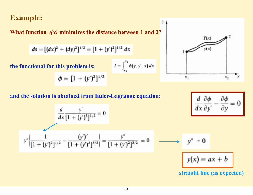
Example:

What function y(x) minimizes the distance between 1 and 2?

the functional for this problem is:

and the solution is obtained from Euler-Lagrange equation:

straight line (as expected)

84

Connection of what we jus did with variations:

arbitrary functions, satisfying:

infinitesimal

then:

variation of the functional:

Taylor series expansion:

Taylor series expansion about ϵ = 0

85

I(ϵ) has an extremum for ϵ = 0!

arbitrary functions

Euler-Lagrange equation for the variational problem!

partial integrationpartial integration

arbitrary variations

Connection of what we jus did with variations:

86

Hamilton’s principlebased on FW-18

Variational statement of mechanics: (for conservative forces)

actionthe particle takes the path

that minimizes the integrated difference of the kinetic and

potential energiesEquivalent to Newton’s laws!87

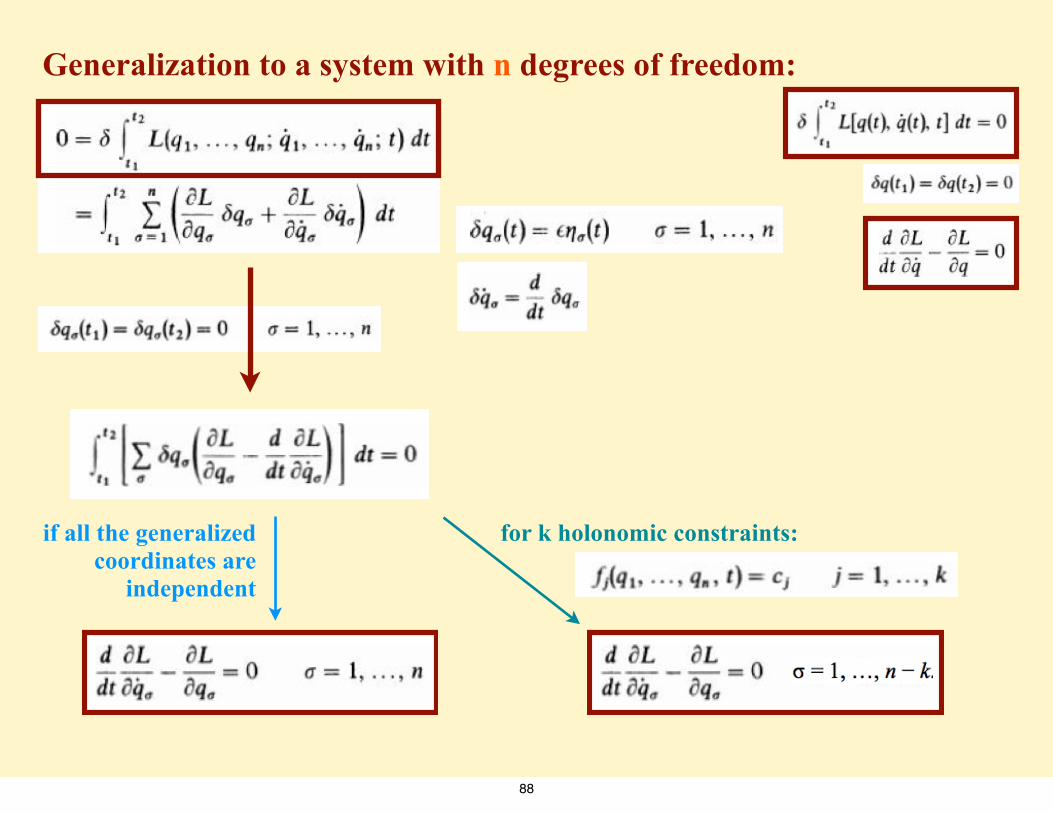
Generalization to a system with n degrees of freedom:

if all the generalized coordinates are

independent

for k holonomic constraints:

88

Forces of constraintbased on FW-19

Often it is useful to incorporate (some) constraints into Hamilton’s principle:

n-k independent coordinates, k constraints

n+k equations for n+k unknowns

adding 0

Lagrange multipliers (can be chosen so that coefficients of k dependent variations of coordinates vanish.

89

Lagrange multipliers determine reaction forces:

Lagrange’s equations:

forces of constraint (reaction forces) (given by Lagrange multipliers)

applied forces

we can choose to include any one or all constraints, solve n+k equations for n+k unknowns, including Lagrange multipliers, and determine reaction forces of interest.

(reaction forces correspond to variations of generalized coordinates that violate the constraints)

90

Using Lagrange’s equationsbased on FW-16

Pendulum:

pendulum equation, small small-amplitude approximation - oscillations with

θ is the generalized coordinate

.θ REVIEW

91

Pendulum: (with r and θ as generalized coordinates)

constraint:

(reaction forces correspond to variations of generalized coordinates

that violate the constraints)

the force of constraint is the tension:

3 eqns. for 3 unknown

pendulum equation

tension force given by the the centrifugal force and the r-component of the gravitational force

92