calculus of variations & optimal control - sasane
TRANSCRIPT

7/27/2019 Calculus of Variations & Optimal Control - Sasane
http://slidepdf.com/reader/full/calculus-of-variations-optimal-control-sasane 1/63
Calculus of Variations and Optimal Control
7/27/2019 Calculus of Variations & Optimal Control - Sasane
http://slidepdf.com/reader/full/calculus-of-variations-optimal-control-sasane 2/63
ii
Preface
This pamphlet on calculus of variations and optimal control theory contains the most important results in the subject, treated largely in order of urgency. Familiarity with linear algebra andreal analysis are assumed. It is desirable, although not mandatory, that the reader has also had acourse on differential equations. I would greatly appreciate receiving information about any errornoticed by the readers. I am thankful to Dr. Sara Maad from the University of Virginia, U.S.A.for several useful discussions.
Amol Sasan6 September, 2004
7/27/2019 Calculus of Variations & Optimal Control - Sasane
http://slidepdf.com/reader/full/calculus-of-variations-optimal-control-sasane 3/63
Course description of MA305: Control Theory
Lecturer: Dr. Amol Sasane
Overview
This a high level methods course centred on the establishment of a calculus appropriate tooptimisation problems in which the variable quantity is a function or curve. Such a curve migdescribe the evolutionover continuous time of the state of a dynamical system. This is typical of models of consumor production in economics and financial mathematics (and for models in many other disciplisuch as engineering and physics).The emphasis of the course is on calculations, but there is also some theory.
Aims
The aim of this course is to introduce students to the types of problems encountered in optimcontrol, to provide techniques to analyse and solve these problems, and to provide examples where these techniques are used in practice.
Learning Outcomes
After having followed this course, students should
* have knowledge and understanding of important definitions, concepts and results,and how to apply these in different situations;* have knowledge of basic techniques and methodologies in the topics covered below;* have a basic understanding of the theoretical aspects of the concepts and methodologies
covered;* be able to understand new situations and definitions;* be able to think critically and with sufficient mathematical rigour;* be able to express arguments clearly and precisely.
The course will cover the following content:
1. Examples of Optimal Control Problems.
2. Normed Linear Spaces and Calculus of Variations.
3. Euler-Lagrange Equation.
4. Optimal Control Problems with Unconstrained Controls.
5. The Hamiltonian and Pontryagin Minimum Principle.

7/27/2019 Calculus of Variations & Optimal Control - Sasane
http://slidepdf.com/reader/full/calculus-of-variations-optimal-control-sasane 4/63
7/27/2019 Calculus of Variations & Optimal Control - Sasane
http://slidepdf.com/reader/full/calculus-of-variations-optimal-control-sasane 5/63
vi Contents
4.4 Constraint on the state at final time. Controllability . . . . . . . . . . . . . . . . . 43
5 Optimality principle and Bellman’s equation 47
5.1 The optimality principle . . . . . . . . . . . . . . . . . . . . . . . . . . . . . . . . . 47
5.2 Bellman’s equation . . . . . . . . . . . . . . . . . . . . . . . . . . . . . . . . . . . . 49
Bibliography 55
Index 57

7/27/2019 Calculus of Variations & Optimal Control - Sasane
http://slidepdf.com/reader/full/calculus-of-variations-optimal-control-sasane 6/63

7/27/2019 Calculus of Variations & Optimal Control - Sasane
http://slidepdf.com/reader/full/calculus-of-variations-optimal-control-sasane 7/63
2 Chapter 1. Introduction
x(t) ∈ Rn, u(t) ∈ Rm. So written out, equation (1.1) is the set of equations
dx1
dt(t) = f 1(x1(t), . . . , xn(t), u1(t), . . . , um(t)), x1(ti) = xi,1
...dxn
dt(t) = f n(x1(t), . . . , xn(t), u1(t), . . . , um(t)), xn(ti) = xi,n,
where f 1, . . . , f n denote the components of f . In (1.1), u is the free variable, called the input , whichis usually assumed to be piecewise continuous1. Let the class of Rm-valued piecewise continuousfunctions be denoted by U . Under some regularity conditions on the function f : Rn ×Rm → Rn,there exists a unique solution to the differential equation (1.1) for every initial condition xi ∈ Rnand every piecewise continuous input u:
Theorem 1.2.1 Suppose that f is continuous in both variables. If there exist K > 0, r > 0 and tf > ti such that
f (x2, u(t))
−f (x1, u(t))
≤K
x2
−x1
(1.2)
for all x1, x2 ∈ B(xi, r) = {x ∈ Rn | x − xi ≤ r} and for all t ∈ [ti, tf ], then (1.2) has a
unique solution x(·) in the interval [ti, tm], for some tm > ti. Furthermore, this solution depends continuously on xi for fixed t and u.
Remarks.
1. Continuous dependence on the initial condition is very important, since some inaccuracyis always present in practical situations. We need to know that if the initial conditions areslightly changed, the solution of the differential equation will change only slightly. Otherwise,
slight inaccuracies could yield very different solutions.
2. x is called the state and (1.1) is called the state equation .
3. Condition (1.2) is called the Lipschitz condition .
The above theorem guarantees that a solution exists and that it is unique, but it does not giveany insight into the size of the time interval on which the solutions exist. The following theoremsheds some light on this.
Theorem 1.2.2 Let r > 0 and define Br =
{u
∈U
| u(t)
≤r for all t
}. Suppose that f is
continuously differentiable in both variables. For every xi ∈ Rn, there exists a unique tm(xi) ∈(ti, +∞] such that for every u ∈ Br, (1.1) has a unique solution x(·) in [ti, tm(xi)).
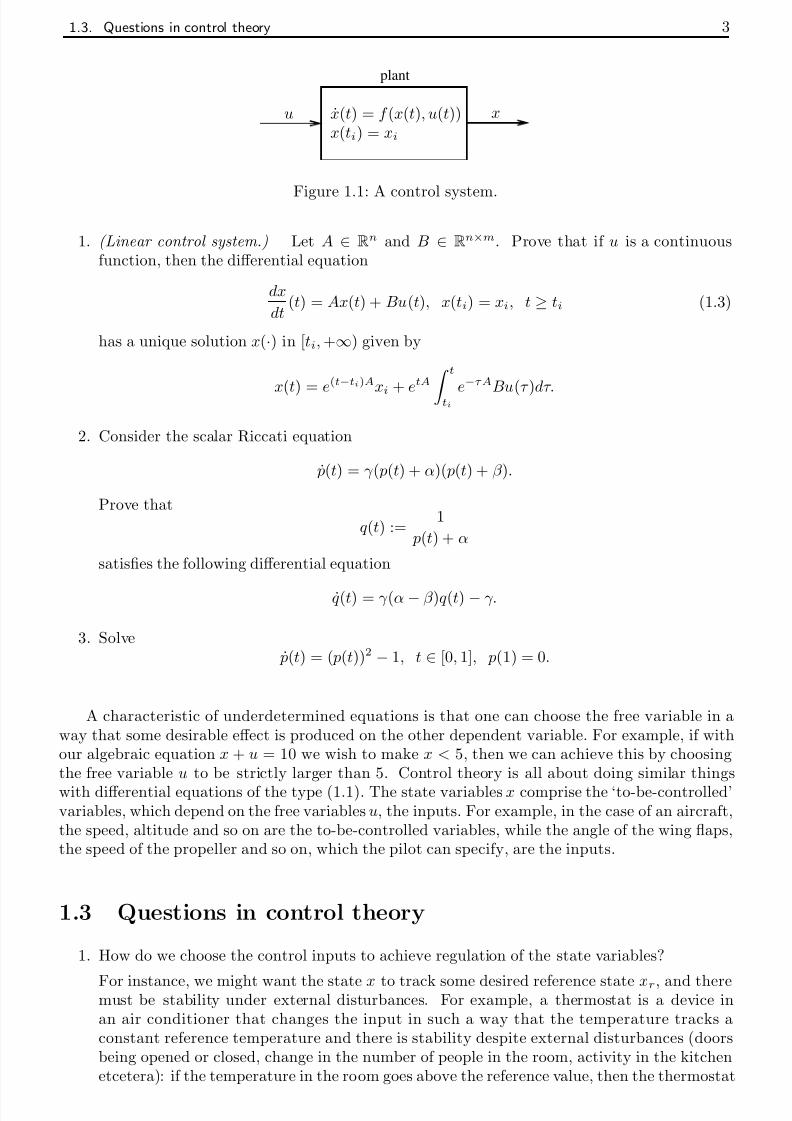
For our purposes, a control system is an equation of the type (1.1), with input u and statex. Once the input u and the intial state x(ti) = xi are specified, the state x is determined. Soone can think of a control system as a box, which given the input u and intial state x(ti) = xi,manufactures the state according to the law (1.1); see Figure 1.1.
If the function f is linear, that is, if f (x, u) = Ax + Bu for some A ∈ Rn×n and B ∈ R
n×m,then the control system is said to be linear .
Exercises.
7/27/2019 Calculus of Variations & Optimal Control - Sasane
http://slidepdf.com/reader/full/calculus-of-variations-optimal-control-sasane 8/63
1.3. Questions in control theory 3
plant
x(t) = f (x(t), u(t))x(ti) = xi
u x
Figure 1.1: A control system.
1. (Linear control system.) Let A ∈ Rn and B ∈ Rn×m. Prove that if u is a continuousfunction, then the differential equation
dx
dt(t) = Ax(t) + Bu(t), x(ti) = xi, t ≥ ti (1.3)
has a unique solution x(·) in [ti, +∞) given by
x(t) = e
(t−ti)A
xi + e
tA tti e
−τA
Bu(τ )dτ.
2. Consider the scalar Riccati equation
˙ p(t) = γ ( p(t) + α)( p(t) + β ).
Prove that
q (t) :=1
p(t) + α
satisfies the following differential equation
q (t) = γ (α − β )q (t) − γ.
3. Solve˙ p(t) = ( p(t))2 − 1, t ∈ [0, 1], p(1) = 0.
A characteristic of underdetermined equations is that one can choose the free variable in away that some desirable effect is produced on the other dependent variable. For example, if withour algebraic equation x + u = 10 we wish to make x < 5, then we can achieve this by choosingthe free variable u to be strictly larger than 5. Control theory is all about doing similar thingswith differential equations of the type (1.1). The state variables x comprise the ‘to-be-controlled’variables, which depend on the free variables u, the inputs. For example, in the case of an aircraft,the speed, altitude and so on are the to-be-controlled variables, while the angle of the wing flaps,the speed of the propeller and so on, which the pilot can specify, are the inputs.
1.3 Questions in control theory
1. How do we choose the control inputs to achieve regulation of the state variables?
For instance, we might want the state x to track some desired reference state xr, and theremust be stability under external disturbances. For example, a thermostat is a device in
i di i h h h i i h h h k
7/27/2019 Calculus of Variations & Optimal Control - Sasane
http://slidepdf.com/reader/full/calculus-of-variations-optimal-control-sasane 9/63
4 Chapter 1. Introduction
(which is a bimetallic strip) bends and closes the circuit so that electricity flows and the airconditioner produces a cooling action; on the other hand if the temperature in the roomdrops below the reference value, the bimetallic strip bends the other way hence breaking thecircuit and the air conditioner produces no further cooling. These problems of regulationare mostly the domain of control theory for engineering systems. In economic systems, oneis furthermore interested in extreme performances of control systems. This naturally brings
us to the other important question in control theory, which is the realm of optimal control theory .
2. How do we control optimally?
Tools from calculus of variations are employed here. These questions of optimality arisenaturally. For example, in the case of an aircraft, we are not just interested in flying fromone place to another, but we would also like to do so in a way so that the total travel timeis minimized or the fuel consumption is minimized. With our algebraic equation x + u = 10,in which we want x < 5, suppose that furthermore we wish to do so in manner such thatu is the least possible integer. Then the only possible choice of the (input) u is 6. Optimalcontrol addresses similar questions with differential equations of the type (1.1), together with
a ‘performance index functional’, which is a function that measures optimality.
This course is about the basic principles behind optimal control theory.
1.4 Appendix: systems of differential equations and etA
In this appendix, we introduce the exponential of a matrix, which is useful for obtaining explicitsolutions to the linear control system (1.3) in the exercise 1 on page 3. We begin with a few
preliminaries concerning vector-valued functions.
With a slight abuse of notation, a vector-valued function x(t) is a vector whose entries arefunctions of t. Similarly, a matrix-valued function A(t) is a matrix whose entries are functions:⎡
⎢⎣x1(t)
...xn(t)
⎤⎥⎦ , A(t) =
⎡⎢⎣
a11(t) . . . a1n(t)...
...am1(t) . . . amn(t)
⎤⎥⎦ .
The calculus operations of taking limits, differentiating, and so on are extended to vector-valuedand matrix-valued functions by performing the operations on each entry separately. Thus by
definition,
limt→t0
x(t) =
⎡⎢⎣
limt→t0 x1(t)...
limt→t0 xn(t)
⎤⎥⎦ .
So this limit exists iff limt→t0 xi(t) exists for all i ∈ {1, . . . , n}. Similiarly, the derivative of a vector-valued or matrix-valued function is the function obtained by differentiating each entryseparately:
dx
dt(t) =
⎡⎢⎣
x1(t)...
xn(t)
⎤⎥⎦ ,
dA
dt(t) =
⎡⎢⎣
a11(t) . . . a1n(t)...
...
am1(t) . . . amn(t)
⎤⎥⎦ ,
where x(t) is the derivative of x (t) and so on So dx is defined iff each of the functions x (t) is

7/27/2019 Calculus of Variations & Optimal Control - Sasane
http://slidepdf.com/reader/full/calculus-of-variations-optimal-control-sasane 10/63
1.4. Appendix: systems of differential equations and etA 5
Here x(t + h) − x(t) is computed by vector addition and the h in the denominator stands forscalr multiplication by h−1. The limit is obtained by evaluating the limit of each entry separately,as above. So the entries of (1.4) are the derivatives xi(t). The same is true for matrix-valuedfunctions.
A system of homogeneous, first-order, linear constant-coefficient differential equations is amatrix equation of the form
dx
dt(t) = Ax(t), (1.5)
where A is a n × n real matrix and x(t) is an n dimensional vector-valued function. Writing outsuch a system, we obtain a system of n differential equations, of the form
dx1
dt(t) = a11x1(t) + · · · + a1nxn(t)
. . .dxn
dt(t) = an1x1(t) + · · · + annxn(t).
The xi(t) are unknown functions, and the aij are scalars. For example, if we substitute the matrix3 −21 4
for A, (1.5) becomes a system of two equations in two unknowns:
dx1
dt(t) = 3x1(t) − 2x2(t)
dx2
dt(t) = x1(t) + 4x2(t).
Now consider the case when the matrix A is simply a scalar. We learn in calculus that thesolutions to the first-order scalar linear differential equation
dx
dt(t) = ax(t)
are x(t) = ceta, c being an arbitrary constant. Indeed, ceta obviously solves this equation. Toshow that every solution has this form, let x(t) be an arbitrary differentiable function which is asolution. We differentiate e−tax(t) using the product rule:
ddt
(e−tax(t)) = −ae−tax(t) + e−taax(t) = 0.
Thus e−tax(t) is a constant, say c, and x(t) = ceta. Now suppose that analogous to
ea = 1 + a +a2
2!+
a3
3!+ . . . , a ∈ R,
we define
eA = I + A +1
2!A2 +
1
3!A3 + . . . , A ∈ Rn×n. (1.6)
Later in this section, we study this matrix exponential, and use the matrix-valued function
tA I tAt2
A2 t3A2

7/27/2019 Calculus of Variations & Optimal Control - Sasane
http://slidepdf.com/reader/full/calculus-of-variations-optimal-control-sasane 11/63
6 Chapter 1. Introduction
Theorem 1.4.1 The series (1.6) converges for any given square matrix A.
We have collected the proofs together at the end of this section in order to not break up thediscussion.
Since matrix multiplication is relatively complicated, it isn’t easy to write down the matrix
entries of eA directly. In particular, the entries of eA are usually not obtained by exponentiatingthe entries of A. However, one case in which the exponential is easily computed, is when A isa diagonal matrix, say with diagonal entries λi. Inspection of the series shows that eA is alsodiagonal in this case and that its diagonal entries are eλi .
The exponential of a matrix A can also be determined when A is diagonalizable , that is,whenever we know a matrix P such that P −1AP is a diagonal matrix D. Then A = P DP −1, andusing (P DP −1)k = P DkP −1, we obtain
eA = I + A +1
2!A2 +
1
3!A3 + . . .
= I + P DP −1 +1
2!
2
P D2P −1 +1
3!P D3P −1 + . . .
= P IP − + P DP −1 +1
2!
2
P D2P −1 +1
3!P D3P −1 + . . .
= P
I + D +
1
2!D2 +
1
3!D3 + . . .
P −1
= P eDP −1
= P ⎡⎢⎣eλ1
0. . .
eλn⎤⎥⎦P −1,
where λ1, . . . , λn denote the eigenvalues of A.
Exercise. (∗) The set of diagonalizable n × n real matrices is dense in the set of all n × n realmatrices, that is, given any A ∈ Rn×n, there exists a B ∈ Rn×n arbitrarily close to A (meaningthat |bij − aij | can be made arbitrarily small for all i, j ∈ {1, . . . , n}) such that B has n distincteigenvalues.
In order to use the matrix exponential to solve systems of differential equations, we need toextend some of the properties of the ordinary exponential to it. The most fundamental propertyis ea+b = eaeb. This property can be expressed as a formal identity between the two infinite serieswhich are obtained by expanding
ea+b = 1 + (a+b)1!
+ (a+b)2
2!+ . . . and
eaeb =
1 + a1!
+ a2
2!+ . . .
1 + b
1!+ b2
2!+ . . .
.
(1.7)
We cannot substitute matrices into this identity because the commutative law is needed to obtainequality of the two series. For instance, the quadratic terms of (1.7), computed without the
commutative law, are 12 (a2 + ab + ba + b2) and 1
2a2 + ab + 12b2. They are not equal unless ab = ba.
So there is no reason to expect eA+B to equal eAeB in general. However, if two matrices A and
7/27/2019 Calculus of Variations & Optimal Control - Sasane
http://slidepdf.com/reader/full/calculus-of-variations-optimal-control-sasane 12/63
1.4. Appendix: systems of differential equations and etA 7
The proof is at the end of this section. Note that the above implies that eA is always invertibleand in fact its inverse is e−A: Indeed I = eA−A = eAe−A.
Exercises.
1. Give an example of 2 × 2 matrices A and B such that e
A+B
= e
A
e
B
.2. Compute eA, where A is given by
A =
2 30 2
.
Hint: A = 2I +
0 30 0
.
We now come to the main result relating the matrix exponential to differential equations.Given an n × n matrix, we consider the exponential etA, t being a variable scalar, as a matrix-valued function:
etA = I + tA +t2
2!A2 +
t3
3!A3 + . . . .
Theorem 1.4.3 etA is a differentiable matrix-valued function of t, and its derivative is etA.
The proof is at the end of the section.
Theorem 1.4.4 (Product rule.) Let A(t) and B(t) be differentiable matrix-valued functions of t,of suitable sizes so that their product is defined. Then the matrix product A(t)B(t) is differentiable,and its derivative is
d
dt(A(t)B(t)) =
dA(t)
dtB(t) + A(t)
dB(t)
dt.
The proof is left as an exercise.
Theorem 1.4.5 The first-order linear differential equation
dx
dt(t) = Ax(t), t ≥ ti, x(ti) = xi
has the unique solution x(t) = e(t−ti)Axi.
Proof

7/27/2019 Calculus of Variations & Optimal Control - Sasane
http://slidepdf.com/reader/full/calculus-of-variations-optimal-control-sasane 13/63
Chapter 2
The optimal control problem
2.1 Introduction
Optimal control theory is about controlling the given system in some ‘best’ way. The optimalcontrol strategy will depend on what is defined as the best way. This is usually specified in termsof a performance index functional.
As a simple example, consider the problem of a rocket launching a satellite into an orbit aboutthe earth. An associated optimal control problem is to choose the controls (the thrust attitudeangle and the rate of emission of the exhaust gases) so that the rocket takes the satellite into its
prescribed orbit with minimum expenditure of fuel or in minimum time.
We first look at a number of specific examples that motivate the general form for optimalcontrol problems, and having seen these, we give the statement of the optimal control problemthat we study in these notes in §2.4.
2.2 Examples of optimal control problems
Example. (Economic growth.) We first consider a mathematical model of a simplified economy
in which the rate of output Y is assumed to depend on the rates of input of capital K (for examplein the form of machinery) and labour force L, that is,
Y = P (K, L)
where P is called the production function. This function is assumed to have the following ‘scaling’property
P (αK, αL) = αP (K, L).
With α = 1L
, and defining the output rate per worker as y = Y L
and the capital rate per worker
as k = K L
, we have
y =Y
L= 1
LP (K, L) = P
K
L,
L
L
= P (k, 1) = Π(k), say.

7/27/2019 Calculus of Variations & Optimal Control - Sasane
http://slidepdf.com/reader/full/calculus-of-variations-optimal-control-sasane 14/63
10 Chapter 2. The optimal control problem
Π
k
Figure 2.1: Production function Π.
where C and I are the rates of consumption and investment, respectively.
The investment is used to increase the capital stock and replace machinery, that is
I (t) =dK
dt (t) + μK (t),
where μ is called the rate of depreciation. Defining c = C L
as the consumption rate per worker, weobtain
y(t) = Π(k(t)) = c(t) +1
L(t)
dK
dt(t) + μk(t).
Sinced
dt
K
L
=
1
L
dK
dt− k
L
dL
dt,
it follows that
Π(k) = c + dkdt
+˙
LL
k + μk.
Assuming that labour grows exponentially, that is L(t) = L0eλt, we have
dk
dt(t) = Π(k(t)) − (λ + μ)k(t) − c(t),
which is the governing equation of this economic growth model. The consumption rate per worker,namely c, is the control input for this problem.
The central planner’s problem is to choose c on a time interval [0, T ] in some best way. Butwhat are the desired economic objectives that define this best way? One method of quantifying
the best way is to introduce a ‘utility’ function U ; which is a measure of the value attachedto the consumption. The function U normally satisfies U (c) ≤ 0, which means that a fixedincrement in consumption will be valued increasingly highly with decreasing consumption level.This is illustrated in Figure 2.2. We also need to optimize consumption for [0 , T ], but with somediscounting for future time. So the central planner wishes to maximize the ‘welfare’ integral
W (c) =
T 0
e−δtU (c(t))dt,
where δ is known as the discount rate, which is a measure of preference for earlier rather thanlater consumption. If δ = 0, then there is no time discounting and consumption is valued equally
at all times; as δ increases, so does the discounting of consumption and utility at future times.
The athe atical oble has o bee ed ced to fi di g the o ti al co s tio ath

7/27/2019 Calculus of Variations & Optimal Control - Sasane
http://slidepdf.com/reader/full/calculus-of-variations-optimal-control-sasane 15/63
2.2. Examples of optimal control problems 11
U
c
Figure 2.2: Utility function U .
and with k(0) = k0.
Example. (Exploited populations.) Many resources are to some extent renewable (for example,fish populations, grazing land, forests) and a vital problem is their optimal management. With
no harvesting, the resource population x is assumed to obey a growth law of the form
dx
dt(t) = ρ(x(t)). (2.1)
A typical example for ρ is the Verhulst model
ρ(x) = ρ0x
1 − x
xs
,
where xs is the saturation level of population, and ρ0 is a positive constant. With harvesting,(2.1) is modified to
dx
dt(t) = ρ(x(t)) − h(t)
where h is the harvesting rate. Now h will depend on the fishing effort e (for example, size of nets,number of trawlers, number of fishing days) as well as the population level, so that we assume
h(t) = e(t)x(t).
Optimal management will seek to maximize the economic rent defined by
r(t) = ph(t) − ce(t),
assuming the cost to be proportional to the effort, and where p is the unit price.
The problem is to maximize the discounted economic rent, called the present value V , oversome period [0, T ], that is,
V (e) = T
0
e−δt( pe(t)x(t) − ce(t))dt,
subject to
7/27/2019 Calculus of Variations & Optimal Control - Sasane
http://slidepdf.com/reader/full/calculus-of-variations-optimal-control-sasane 16/63
12 Chapter 2. The optimal control problem
2.3 Functionals
The examples from the previous section involve finding extremum values of integrals subject to adifferential equation constraint. These integrals are particular examples of a ‘functional’.
A functional is a correspondence which assigns a definite real number to each function be-
longing to some class. Thus, one might say that a functional is a kind of function, where theindependent variable is itself a function.
Examples. The following are examples of functionals:
1. Consider the set of all rectifiable plane curves1. A definite number associated with each suchcurve, is for instance, its length. Thus the length of a curve is a functional defined on theset of rectifiable curves.
2. Let x be an arbitrary continuously differentiable function defined on [ti, tf ]. Then the formula
I (x) =
tf ti
dx
dt(t)
2
dt
defines a functional on the set of all such functions x.
3. As a more general example, let F (x, x, t) be a continuous function of three variables. Thenthe expression
I (x) = tf
ti
F x(t),dx
dt(t), t dt,
where x ranges over the set of all continuously differentiable functions defined on the interval[ti, tf ], defines a functional.
By choosing different functions F , we obtain different functionals. For example, if
F (x, x, t) =
1 + (x)2,
then I (x) is the length of the curve {x(t), t ∈ [ti, tf ]}, as in the first example, while if
F (x, x, t) = (x)2,
then I (x) reduces to the case considered in the second example.
4. Let f (x, u) and F (x, u, t) be continuously differentiable functions of their arguments. Givena continuous function u on [ti, tf ], let x denote the unique solution of
dx
dt(t) = f (x(t), u(t)), x(ti) = xi, t ∈ [ti, tf ].
Then I given by
I xi(u) = tf
ti
F (x(t), u(t), t)dt
defines a functional on the set of all continuous functions u on [ti tf ]

7/27/2019 Calculus of Variations & Optimal Control - Sasane
http://slidepdf.com/reader/full/calculus-of-variations-optimal-control-sasane 17/63
2.4. The general form of the basic optimal control problem 13
Exercise. (A path-independent functional.) Consider the set of all continuously differentiablefunctions x defined on [ti, tf ] such that x(ti) = xi and x(tf ) = xf , and let
I (x) =
tf ti
x(t) + t
dx
dt(t)
dt.
Show that I is independent of path. What is its value?
Remark. Such a functional is analogous to the notion of a constant function f : R → R, forwhich the problem of finding extremal points is trivial: indeed since the value is constant, everypoint serves as a point which maximizes/minimizes the functional.
2.4 The general form of the basic optimal control problem
The examples discussed in §2.2 can be put in the following form. As mentioned in the introduction,
we assume that the state of the system satisfies the coupled first order differential equationsdx1
dt(t) = f 1(x1(t), . . . , xn(t), u1(t), . . . , um(t)), x1(t0) = xi,1
...dxn
dt(t) = f n(x1(t), . . . , xn(t), u1(t), . . . , um(t)), xn(t0) = xi,n,
on [ti, tf ], and where the m variables u1, . . . , um form the control input vector u. We can conve-niently write the system of equations above in the form
dxdt
(t) = f (x(t), u(t)), x(ti) = xi, t ∈ [ti, tf ].
We assume that u ∈ (C [ti, tf ])m, that is, each component of u is a continuous function on [ti, tf ].
It is also assumed that f 1, . . . , f n possess partial derivatives with respect to xk, 1 ≤ k ≤ n andul, 1 ≤ l ≤ m and these are continuous. (So f is continuously differentiable in both variables.)The initial value of x is specified (xi at time ti), which means that specifying u(t) for t ∈ [ti, tf ]determines x (see Theorem 1.2.1).
The basic optimal control problem is to choose the control u ∈ (C [ti, tf ])m such that:
1. The state x is transferred from xi to a state at terminal time tf where some (or all or none)of the state variable components are specified; for example, without loss of generality2 x(tf )kis specified for k ∈ {1, . . . , r}.
2. The functional
I xi(u) =
tf ti
F (x(t), u(t), t)dt
is minimized3.
A function u∗ that minimizes the functional I is called an optimal control , the corresponding statex∗ is called the optimal state , and the pair (x∗, u∗) is called an optimal trajectory . Using the
i b id if h i l l bl l li d i §2 2
7/27/2019 Calculus of Variations & Optimal Control - Sasane
http://slidepdf.com/reader/full/calculus-of-variations-optimal-control-sasane 18/63
14 Chapter 2. The optimal control problem
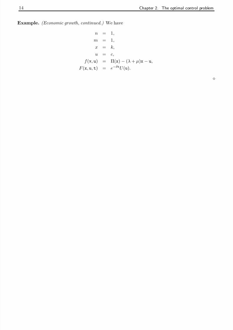
Example. (Economic growth, continued.) We have
n = 1,
m = 1,
x = k,
u = c,
f (x, u) = Π(x) − (λ + μ)x − u,
F (x, u, t) = e−δtU (u).

7/27/2019 Calculus of Variations & Optimal Control - Sasane
http://slidepdf.com/reader/full/calculus-of-variations-optimal-control-sasane 19/63
Chapter 3
Calculus of variations
3.1 Introduction
Before we attempt solving the optimal control problem described in Section 2.4 of Chapter 2,that is, an extremum problem for a functional of the type described in item 4 on page 12, weconsider the following simpler problem in this chapter: we would like to find extremal curves x fora functional of the type described in item 3 on page 12. This is simpler since there is no differentialequation constraint.
In order to solve this problem, we first make the problem more abstract by considering the
problem of finding extremal points x∗ ∈ X for a functional I : X → R, where X is a normed linearspace. (The notion of a normed linear space is introduced in Section 3.4.) We develop a calculusfor solving such problems. This situation is entirely analogous to the problem of finding extremalpoints for a differentiable function f : R → R:
Consider for example the quadratic function f (x) = ax2 + bx + c. Suppose that one wantsto know the points x∗ at which f assumes a maximum or a minimum. We know that if f hasa maximum or a minimum at the point x∗, then the derivative of the function must be zero atthat point: f (x∗) = 0. See Figure 3.1. So one can then one can proceed as follows. First findthe expression for the derivative: f (x) = 2ax + b. Next solve for the unknown x∗ in the equationf (x∗) = 0, that is,
2ax∗ + b = 0 (3.1)
and so we find that a candidate for the point x∗ which minimizes or maximizes f is x∗ = − b2a
,which is obtained by solving the algebraic equation (3.1) above.
x xx∗x∗
f f
Figure 3.1: Necessary condition for x∗ to be an extremal point for f is that f (x∗) = 0.

7/27/2019 Calculus of Variations & Optimal Control - Sasane
http://slidepdf.com/reader/full/calculus-of-variations-optimal-control-sasane 20/63
16 Chapter 3. Calculus of variations
at extremal points. We define the derivative of a functional I : X → R in Section 3.4, and alsoprove Theorem 3.4.2, which says that this derivative must vanish at an extremal point x∗ ∈ X .
In the remainder of the chapter, we apply Theorem 3.4.2 to the concrete case where X com-prises continuously differentiable functions, and I is a functional of the form
I (x) = tf ti F (x(t), x
(t), t)dt. (3.2)
We find the derivative of such a functional, and equating it to zero, we obtain a necessary condi-tion that an extremal curve should satisfy: instead of an algebraic equation (3.1), we now obtaina differential equation, called the Euler-Lagrange equation, given by (3.9). Continuously differen-tiable solutions x∗ of this differential equation are then candidates which maximize or minimizethe functional I . Historically speaking, such optimization problems arising from physics gave birthto the subject of ‘calculus of variations’. We begin this chapter with the discussion of one suchmilestone problem, called the ‘brachistochrone problem’ (brachistos=shortest, chronos=time).
3.2 The brachistochrone problem
The calculus of variations originated from a problem posed by the Swiss mathematician JohannBernoulli (1667-1748). He required the form of the curve joining two fixed points A and B in avertical plane such that a body sliding down the curve (under gravity and no friction) travels fromA to B in minimum time. This problem does not have a trivial solution; the straight line from A
to B is not the solution (this is also intuitively clear, since if the slope is high at the beginning,the body picks up a high velocity and so its plausible that the travel time could be reduced) andit can be verified experimentally by sliding beads down wires in appropriate shapes.
To pose the problem in mathematical terms, we introduce coordinates as shown in Figure 3.2,so that A is the point (0, 0), and B corresponds to (x0, y0). Assuming that the particle is released
A (0, 0)
B (x0, y0)
gravity
y0
x0
x
y
Figure 3.2: The brachistochrone problem.
from rest at A, conservation of energy gives
1
2mv2 − mgy = 0, (3.3)
where we have taken the zero potential energy level at y = 0, and where v denotes the speed of
the particle. Thus the speed is given by
ds

7/27/2019 Calculus of Variations & Optimal Control - Sasane
http://slidepdf.com/reader/full/calculus-of-variations-optimal-control-sasane 21/63
3.3. Calculus of variations versus extremum problems of functions of n real variables 17
δy
δx
δs
Figure 3.3: Element of arc length.
T =
curve
ds√ 2gy
=1√ 2g
y00
⎡⎢⎣1 +
dxdy
2y
⎤⎥⎦
12
dy.
Our problem is to find the path {x(y), y ∈ [0, y0]}, satisfying x(0) = 0 and x(y0) = x0, whichminimizes T .
3.3 Calculus of variations versus extremum problems of functions of n real variables
To understand the basic meaning of the problems and methods of the calculus of variations, it isimportant to see how they are related to the problems of the study of functions of n real variables.Thus, consider a functional of the form
I (x) =
tf ti
F
x(t),
dx
dt(t), t
dt, x(ti) = xi, x(tf ) = xf .
Here each curve x is assigned a certain number. To find a related function of the sort consideredin classical analysis, we may proceed as follows. Using the points
ti = t0, t1, . . . , tn, tn+1 = tf ,
we divide the interval [ti, tf ] into n + 1 equal parts. Then we replace the curve {x(t), t ∈ [ti, tf ]}by the polygonal line joining the points
(t0, xi), (t1, x(t1)), . . . , (tn, x(tn)), (tn+1, xf ),
and we approximate the functional I at x by the sum
I n(x1, . . . , xn) =nk=1
F
xk,
xk − xk−1
hk, tk
hk, (3.5)
where xk = x(tk) and hk = tk− tk−1. Each polygonal line is uniquely determined by the ordinatesx1, . . . , xn of its vertices (recall that x0 = xi and xn+1 = xf are fixed), and the sum (3.5) istherefore a function of the n variables x1, . . . , xn. Thus as an approximation, we can regard thevariational problem as the problem of finding the extrema of the function I n(x1, . . . , xn).
In solving variational problems, Euler made extensive use of this ‘method of finite differences’.
By replacing smooth curves by polygonal lines, he reduced the problem of finding extrema of afunctional to the problem of finding extrema of a function of n variables, and then he obtained
l i b i h li i I hi f i l b d d
7/27/2019 Calculus of Variations & Optimal Control - Sasane
http://slidepdf.com/reader/full/calculus-of-variations-optimal-control-sasane 22/63
18 Chapter 3. Calculus of variations
3.4 Calculus in function spaces and beyond
In the study of functions of a finite number of n variables, it is convenient to use geometriclanguage, by regarding a set of n numbers (x1, . . . , xn) as a point in an n-dimensional space. Inthe same way, geometric language is useful when studying functionals. Thus, we regard eachfunction x(
·) belonging to some class as a point in some space, and spaces whose elements are
functions will be called function spaces.
In the study of functions of a finite number n of independent variables, it is sufficient to considera single space, that is, n-dimensional Euclidean space Rn. However, in the case of function spaces,there is no such ‘universal’ space. In fact, the nature of the problem under consideration determinesthe choice of the function space. For instance, if we consider a functional of the form
I (x) =
tf ti
F
x(t),
dx
dt(t), t
dt,
then it is natural to regard the functional as defined on the set of all functions with a continuousfirst derivative.
The concept of continuity plays an important role for functionals, just as it does for the ordi-nary functions considered in classical analysis. In order to formulate this concept for functionals,we must somehow introduce a notion of ‘closeness’ for elements in a function space. This is mostconveniently done by introducing the concept of the norm of a function, analogous to the conceptof the distance between a point in Euclidean space and the origin. Although in what follows weshall always be concerned with function spaces, it will be most convenient to introduce the conceptof a norm in a more general and abstract form, by introducing the concept of a normed linear space .
By a linear space (or vector space ) over R, we mean a set X together with the operations of addition + : X × X → X and scalar multiplication · : R× X → X that satisfy the following:
1. x1 + (x2 + x3) = (x1 + x2) + x3 for all x1, x2, x3 ∈ X .
2. There exists an element, denoted by 0 (called the zero element ) such that x + 0 = 0 + x = x
for all x ∈ X .
3. For every x ∈ X , there exists an element, denoted by −x such that x + (−x) = (−x) + x = 0.
4. x1 + x2 = x2 + x1 for all x1, x2 ∈ X .
5. 1 · x = x for all x ∈ X .
6. α · (β · x) = (αβ ) · x for all α, β ∈ R and for all x ∈ X .
7. (α + β ) · x = α · x + β · x for all α, β ∈ R and for all x ∈ X .
8. α · (x1 + x2) = α · x1 + α · x2 for all α ∈ R and for all x1, x2 ∈ X .
A linear functional L : X → R is a map that satisfies
7/27/2019 Calculus of Variations & Optimal Control - Sasane
http://slidepdf.com/reader/full/calculus-of-variations-optimal-control-sasane 23/63
3.4. Calculus in function spaces and beyond 19
The set ker(L) = {x ∈ X | L(x) = 0} is called the kernel of the linear functional L.
Exercise. (∗) If L1, L2 are linear functionals defined on X such that ker(L1) ⊂ ker(L2), thenprove that there exists a constant λ ∈ R such that L2(x) = λL1(x) for all x ∈ X .
Hint: The case when L1 = 0 is trivial. For the other case, first prove that if ker(L1)
= X , then
there exists a x0 ∈ X such that X = ker(L1) + [x0], where [x0] denotes the linear span of x0.What is L2x for x ∈ X ?
A linear space over R is said to be normed , if there exists a function · : X → [0, ∞) (callednorm ), such that:
1. x = 0 iff x = 0.
2. α · x = |α| x for all α ∈ R and for all x ∈ X .
3. x1 + x2 ≤ x1 + x2 for all x1, x2 ∈ X . (Triangle inequality.)
In a normed linear space, we can talk about distances between elements, by defining the distancebetween x1 and x2 to be the quantity x1 − x2. In this manner, a normed linear space becomesa metric space. Recall that a metric space is a set X together with a function d : X × X → R,called distance , that satisfies
1. d(x, y) ≥ 0 for all x, y in X , and d(x, y) = 0 iff x = y.
2. d(x, y) = d(y, x) for all x, y in X .
3. d(x, z) ≤ d(x, y) + d(y, z) for all x , y , z in X .
Exercise. Let (X, · ) be a normed linear space. Prove that (X, d) is a metric space, whered : X × X → [0, ∞) is defined by d(x1, x2) = x1 − x2, x1, x2 ∈ X .
The elements of a normed linear space can be objects of any kind, for example, numbers,matrices, functions, etcetera. The following normed spaces are important for our subsequent
purposes:
1. C [ti, tf ].
The space C [ti, tf ] consists of all continuous functions x(·) defined on the closed interval[ti, tf ]. By addition of elements of C [ti, tf ], we mean pointwise addition of functions: forx1, x2 ∈ C [ti, tf ], (x1 + x2)(t) = x1(t) + x2(t) for all t ∈ [ti, tf ]. Scalar multiplication isdefined as follows: (α · x)(t) = αx(t) for all t ∈ [ti, tf ]. The norm is defined as the maximumof the absolute value:
x = maxt∈[ti,tf ]
|x(t)|.
Thus in the space C [ti, tf ], the distance between the function x∗ and the function x does not

7/27/2019 Calculus of Variations & Optimal Control - Sasane
http://slidepdf.com/reader/full/calculus-of-variations-optimal-control-sasane 24/63
20 Chapter 3. Calculus of variations
ti tf
x∗x
t
Figure 3.4: A ball of radius and center x∗ in C [ti, tf ].
The space C 1[ti, tf ] consists of all functions x(·) defined on [ti, tf ] which are continuous andhave a continuous first derivative. The operations of addition and multiplication by scalarsare the same as in C [ti, tf ], but the norm is defined by
x = maxt∈[ti,tf ]
|x(t)| + maxt∈[ti,tf ]
dx
dt(t)
.
Thus two functions in C 1[ti, tf ] are regarded as close together if both the functions themselvesas well as their first derivatives are close together. Indeed this is because x1−x2 < impliesthat
|x1(t) − x2(t)| < and
dx1
dt(t) − dx2
dt(t)
< for all t ∈ [ti, tf ], (3.6)
and conversely, (3.6) implies that x1 − x2 < 2.
Similarly for d ∈ N, we can introduce the spaces (C [ti, tf ])d, (C 1[ti, tf ])
d, the spaces of functionsfrom [ti, tf ] into Rd, whose each component belongs to C [ti, tf ], C 1[ti, tf ], respectively.
After a norm has been introduced in a linear space X (which may be a function space), it isnatural to talk about continuity of functionals defined on X . The functional I : X → R is said tobe continuous at the point x∗ if for every > 0, there exists a δ > 0 such that
|I (x) − I (x∗)| < for all x such that x − x∗ < δ.
The functional I : X → R is said to be continuous if it is continuous at all x ∈ X .
Exercises.
1. (∗) Show that the arclength functional I : C 1[0, 1] → R given by
I (x) =
10
1 + (x(t))2dt
is not continuous if we equip C 1[0, 1] with any of the following norms:
(a) x = maxt∈[0,1] |x(t)|, x ∈ C 1[0, 1].
(b)
x
= maxt∈[0,1] |x(t)
|+ dx
dt
(t).
Hint: One might proceed as follows: consider the curves x(t) = 2 sint
for > 0,
and prove that x → 0 while I(x ) → ∞ as → 0
7/27/2019 Calculus of Variations & Optimal Control - Sasane
http://slidepdf.com/reader/full/calculus-of-variations-optimal-control-sasane 25/63
3.4. Calculus in function spaces and beyond 21
At first it might seem that the space C [ti, tf ] (which is strictly larger than C 1[ti, tf ]) wouldbe adequate for the study of variational problems. However, this is not true. In fact one of thebasic functionals
I (x) =
tf ti
F
x(t),
dx
dt(t), t
dt
is continuous if we interpret closeness of functions as closeness in the space C 1[ti, tf ]. For example,
arc length is continuous if we use the norm in C 1[ti, tf ], but not 1 continuous if we use the normin C [ti, tf ]. Since we want to be able to use ordinary analytic operations such as passage to thelimit, then, given a functional, it is reasonable to choose a function space such that the functionalis continuous.
So far we have talked about linear spaces and functionals defined on them. However, inmany variational problems, we have to deal with functionals defined on sets of functions whichdo not form linear spaces. In fact, the set of functions satisfying the constraints of a givenvariational problem, called the admissible functions is in general not a linear space. For example,the admissible curves for the brachistochrone problem are the smooth plane curves passing throughtwo fixed points, and the sum of two such curves does not in general pass through the two points.Nevertheless, the concept of a normed linear space and the related concepts of the distance betweenfunctions, continuity of functionals, etcetera, play an important role in the calculus of variations.A similar situation is encountered in elementary analysis, where, in dealing with functions of n
variables, it is convenient to use the concept of the n-dimensional Euclidean space Rn, even thoughthe domain of definition of a function may not be a linear subspace of Rn.
Next we introduce the concept of the (Frechet) derivative of a functional, analogous to theconcept of the derivative of a function of n variables. This concept will then be used to findextrema of functionals.
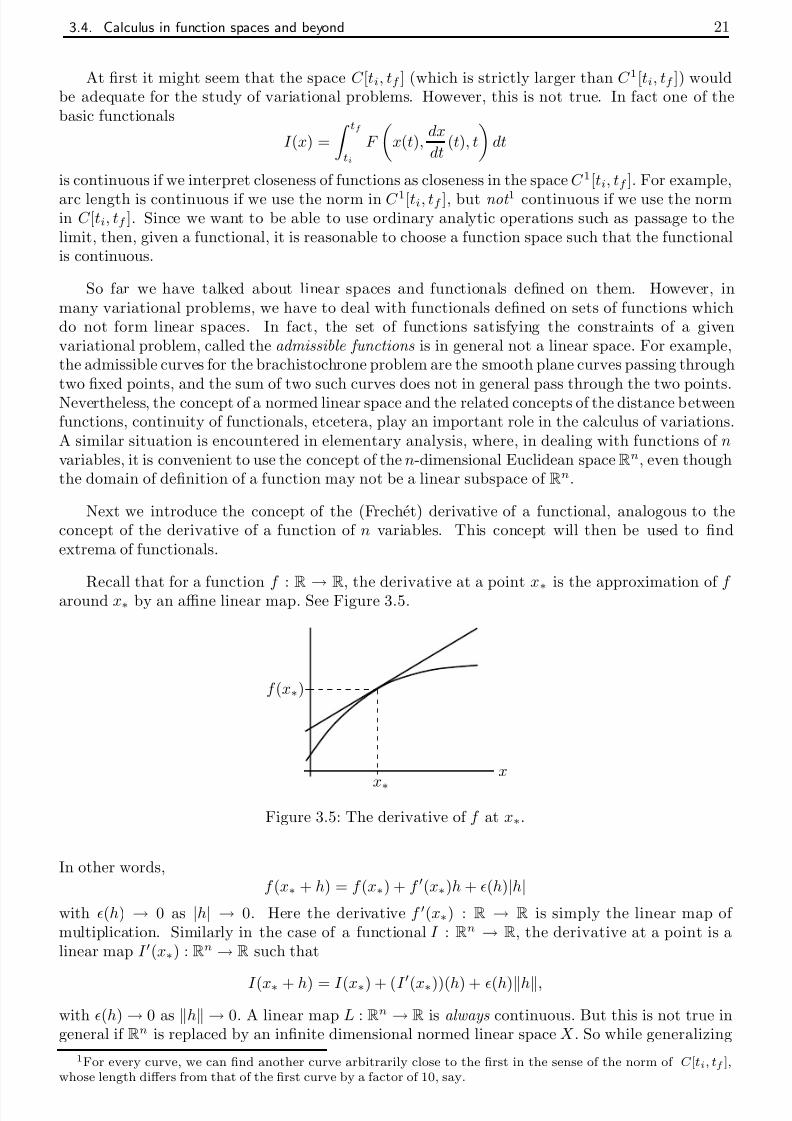
Recall that for a function f :R
→R
, the derivative at a point x∗ is the approximation of f around x∗ by an affine linear map. See Figure 3.5.
f (x∗)
x∗x
Figure 3.5: The derivative of f at x∗.
In other words,f (x∗ + h) = f (x∗) + f (x∗)h + (h)|h|
with (h) → 0 as |h| → 0. Here the derivative f (x∗) : R → R is simply the linear map of multiplication. Similarly in the case of a functional I : Rn → R, the derivative at a point is alinear map I (x∗) : Rn → R such that
I (x∗ + h) = I (x∗) + (I (x∗))(h) + (h)h,
ith (h) 0 as h 0 A linear map L Rn
R is always continuous But this is not true in

7/27/2019 Calculus of Variations & Optimal Control - Sasane
http://slidepdf.com/reader/full/calculus-of-variations-optimal-control-sasane 26/63
22 Chapter 3. Calculus of variations
the notion of the derivative of a functional I : X → R, we specify continuity of the linear mapas well. This motivates the following definition. Let X be a normed linear space. Then a mapL : X → R is said to be a continuous linear functional if it is linear and continuous.
Exercises.
1. Let L : X → R be a linear functional on a normed linear space X . Prove that the followingare equivalent:
(a) L is continuous.
(b) L is continuous at 0.
(c) There exists a M > 0 such that |L(x)| ≤ M x for all x ∈ X .
Hint. The implication (1a)⇒(1b) follows from the definition and (1c)⇒(1a) is easy to proveusing a δ <
M . For (1b)⇒(1c), use M >
δand consider separately the cases x = 0 and
x = 0. In the latter case, note that with x1 :=
M
xx, there holds that x1 < δ .Remark. Thus in the case of linear functionals, remarkably, continuity is equivalent tocontinuity at only one point, and this is furthermore equivalent to proving an estimate of the type given in item 1c.
2. Let tm ∈ [ti, tf ]. Prove that the map L : C [ti, tf ] → R given by L(x) = x(tm) is a continuouslinear functional.
3. Let α, β ∈ C [ti, tf ]. Prove that the map L : C 1[ti, tf ] → R given by
L(x) = tf ti
α(t)x(t) + β (t)
dx
dt (t)
dt
is a continuous linear functional.
We are now ready to define the derivative of a functional. Let X be a normed linear spaceand I : X → R be a functional. Then I is said to be (Frechet) differentiable at x∗ (∈ X ) if thereexists a continuous linear functional, denoted by I (x∗), and a map : X → R such that
I (x∗ + h) = I (x∗) + (I (x∗))(h) + (h)h, for all h ∈ X,
and (h) → 0 as h → 0. Then I (x∗) is called the (Frechet) derivative of I at x∗. If I isdifferentiable at every point x ∈ X , then it is simply said to be differentiable .
Theorem 3.4.1 The derivative of a differentiable functional I : X → R at a point x∗ ( ∈ X ) is unique.
Proof First we note that if L : X → R is a linear functional and if
L(h)
h → 0 as h → 0, (3.7)
1

7/27/2019 Calculus of Variations & Optimal Control - Sasane
http://slidepdf.com/reader/full/calculus-of-variations-optimal-control-sasane 27/63
3.4. Calculus in function spaces and beyond 23
which contradicts (3.7).
Now suppose that the derivative of I at x∗ is not uniquely defined, so that
I (x∗ + h) = I (x∗) + L1(h) + 1(h)h,
I (x∗ + h) = I (x∗) + L2(h) + 2(h)h,
where L1, L2 are continuous linear functionals, and 1(h), 2(h) → 0 as h → 0. Thus
(L1 − L2)(h)
h = 2(h) − 1(h) → 0 as h → 0,
and from the above, it follows that L1 = L2.
Exercises.
1. Prove that if I : X
→R is differentiable at x∗, then it is continuous at x∗.
2. (a) Prove that if L : X → R is a continuous linear functional, then it is differentiable.What is its derivative at x ∈ X ?
(b) Let tm ∈ [ti, tf ]. Consider the functional I : C [ti, tf ] → R given by
I (x) =
tf tm
x(t)dt.
Prove that I is differentiable, and find its derivative at x ∈ C [ti, tf ].
3. (∗) Prove that the square of a differentiable functional I : X → R is differentiable, and find
an expression for its derivative at x ∈ X .4. (a) Given x1, x2 in a normed linear space X , define
ϕ(t) = tx1 + (1 − t)x2.
Prove that if I : X → R is differentiable, then I ◦ ϕ : [0, 1] → R is differentiable and
d
dt(I ◦ ϕ)(t) = [I (ϕ(t))](x1 − x2).
(b) Prove that if I 1, I 2 : X → R are differentiable and their derivatives are equal at every
x ∈ X , then I 1, I 2 differ by a constant.
In elementary analysis, a necessary condition for a differentiable function f : R → R to havea local extremum (local maximum or local minimum) at x∗ ∈ R is that f (x∗) = 0. We willprove a similar necessary condition for a differentiable functional I : X → R. We say that afunctional I : X → R has a local extremum at x∗ (∈ X ) if I (x) − I (x∗) does not change sign insome neighbourhood of x∗.
Theorem 3.4.2 Let I : X → R be a functional that is differentiable at x∗ ∈ X . If I has a local extremum at x∗, then I (x∗) = 0.
Proof To be explicit, suppose that I has a minimum at x∗: there exists r > 0 such that

7/27/2019 Calculus of Variations & Optimal Control - Sasane
http://slidepdf.com/reader/full/calculus-of-variations-optimal-control-sasane 28/63
24 Chapter 3. Calculus of variations
We note that hn → 0 as n → ∞, and so with N chosen large enough, we have hn < r for alln > N . It follows that for n > N ,
0 ≤ I (x∗ + hn) − I (x∗)
hn = −|[I (x∗)](h0)|h0 + (hn).
Passing the limit as n → ∞, we obtain −|[I (x∗)](h0)| ≥ 0, a contradiction.
Remark. Note that this is a necessary condition for the existence of an extremum. Thus a thevanishing of a derivative at some point x∗ doesn’t imply extremality of x∗!
3.5 The simplest variational problem. Euler-Lagrange equa-
tion
The simplest variational problem can be formulated as follows:
Let F (x, x, t) be a function with continuous first and second partial derivatives with respect to(x, x, t). Then find x ∈ C 1[ti, tf ] such that x(ti) = xi and x(tf ) = xf , and which is an extremumfor the functional
I (x) =
tf ti
F
x(t),
dx
dt(t), t
dt. (3.8)
In other words, the simplest variational problem consists of finding an extremum of a functionalof the form (3.13), where the class of admissible curves comprises all smooth curves joining two
fixed points; see Figure 3.6. We will apply the necessary condition for an extremum (established
ti tf
t
xi
xf
Figure 3.6: Possible paths joining the two fixed points (ti, xi) and (tf , xf ).
in Theorem 3.4.2) to the solve the simplest variational problem described above. This will enableus to solve the brachistochrone problem from §3.2.
Theorem 3.5.1 Let I be a functional of the form
I (x) =
tf
ti
F
x(t),
dx
dt(t), t
dt,
where F (x, x, t) is a function with continuous first and second partial derivatives with respect to(x x t) and x ∈ C1[ti tf ] such that x(ti) = xi and x(tf ) = xf If I has an extremum at x then

7/27/2019 Calculus of Variations & Optimal Control - Sasane
http://slidepdf.com/reader/full/calculus-of-variations-optimal-control-sasane 29/63
3.5. The simplest variational problem. Euler-Lagrange equation 25
(This equation is abbreviated by F x − ddt
F x = 0.)
Proof The proof is long and so we divide it into several steps.
Step 1. First of all we note that the set of curves in C 1[ti, tf ] satisfying x(ti) = xi and x(tf ) = xf
do not form a linear space! So Theorem 3.4.2 is not applicable directly. Hence we introduce anew linear space X , and consider a new functional I : X → R which is defined in terms of the oldfunctional I .
Introduce the linear space
X = {h ∈ C 1[ti, tf ] | h(a) = h(b) = 0},
with the C 1[ti, tf ]-norm. Then for all h ∈ X , x∗+h satisfies (x∗+h)(ti) = xi and (x∗+h)(tf ) = xf .
Defining I (h) = I (x∗+h), we note that I : X → R has an extremum at 0. It follows from Theorem3.4.2 that I (0) = 0. Note that by the 0 in the right hand side of the equality, we mean the zero
functional, namely the continuous linear map from X to R, which is defined by h → 0 for allh ∈ X .
Step 2. We now calculate I (0). We have
I (h) − I (0) =
tf ti
F ((x∗ + h)(t), (x∗ + h)(t), t) dt − tf ti
F (x∗(t), x∗(t), t) dt
=
tf ti
[F (x∗(t) + h(t), x∗(t) + h(t), t) dt − F (x∗(t), x∗(t), t)] dt.
Recall that from Taylor’s theorem, if F possesses partial derivatives of order 2 in some neighbour-hood N of (x0, x0, t0), then for all (x, x, t) ∈ N , there exists a Θ ∈ [0, 1] such that
F (x, x, t) = F (x0, x0, t0) +
(x − x0)
∂
∂ x+ (x − x0)
∂
∂ x+ (t − t0)
∂
∂ t
F
(x0,x0,t0)
+
1
2!
(x − x0)
∂
∂ x+ (x − x0)
∂
∂ x+ (t − t0)
∂
∂ t
2
F
(x0,x0,t0)+Θ((x,x,t)−(x0,x0,t0))
.
Hence for h∈
X such that
h
is small enough,
I (h) − I (0) =
tf ti
∂F
∂ x(x∗(t), x∗(t), t) h(t) +
∂F
∂ x(x∗(t), x∗(t), t) h(t)
dt +
1
2!
tf ti
h(t)
∂
∂ x+ h(t)
∂
∂ x
2
F (x∗(t)+Θ(t)h(t),x
∗(t)+Θ(t)h(t),t)
dt.
It can be checked that there exists a M > 0 such that
1
2!
tf
tih(t)
∂
∂ x
+ h(t)∂
∂ x
2
F (x∗(t)+Θ(t)h(t),x
∗(t)+Θ(t)h
(t),t)
dt ≤M
h
2,
( )
7/27/2019 Calculus of Variations & Optimal Control - Sasane
http://slidepdf.com/reader/full/calculus-of-variations-optimal-control-sasane 30/63
26 Chapter 3. Calculus of variations
Step 3. Next we show that if the map in (3.10) is the zero map, then this implies that (3.9)holds. Define
A(t) =
tti
∂F
∂ x(x∗(τ ), x∗(τ ), τ ) dτ.
Integrating by parts, we find that
tf ti
∂F ∂ x
(x∗(t), x∗(t), t) h(t)dt = − tf ti
A(t)h(t)dt,
and so from (3.10), it follows that I (0) = 0 implies that tf ti
−A(t) +
∂F
∂ x(x∗(t), x∗(t), t)
h(t)dt = 0 for all h ∈ X.
Step 4. Finally we will complete the proof by proving the following.
Lemma 3.5.2 If K ∈ C [ti, tf ] and
tf ti
K (t)h(t)dt = 0
for all h ∈ C 1[ti, tf ] with h(ti) = h(tf ) = 0, then there exists a constant k such that K (t) = k for all t ∈ [ti, tf ].
Proof Let k be the constant defined by the condition tf ti
[K (t) − k] dt = 0,
and let
h(t) =
tti
[K (τ ) − k] dτ.
Then h ∈ C 1[ti, tf ] and it satisfies h(ti) = h(tf ) = 0. Furthermore,
tf
ti
[K (t)
−k]
2dt =
tf
ti
[K (t)
−k] h(t)dt =
tf
ti
K (t)h(t)dt
−k(h(tf )
−h(ti)) = 0.
Thus K (t) − k = 0 for all t ∈ [ti, tf ].
Applying Lemma 3.5.2, we obtain
−A(t) +∂F
∂ x(x∗(t), x∗(t), t) = k for all t ∈ [ti, tf ].
Differentiating with respect to t, we obtain (3.10). This completes the proof of Theorem 3.5.1.
Since the Euler-Lagrange equation is in general a second order differential equation, it solu-tion will in general depend on two arbitrary constants, which are determined from the boundary
di i ( ) d ( ) Th bl ll id d i h h f diff
7/27/2019 Calculus of Variations & Optimal Control - Sasane
http://slidepdf.com/reader/full/calculus-of-variations-optimal-control-sasane 31/63
3.5. The simplest variational problem. Euler-Lagrange equation 27
given boundary conditions. Therefore, the question of whether or not a certain variational problemhas a solution does not just reduce to the usual existence theorems for differential equations.
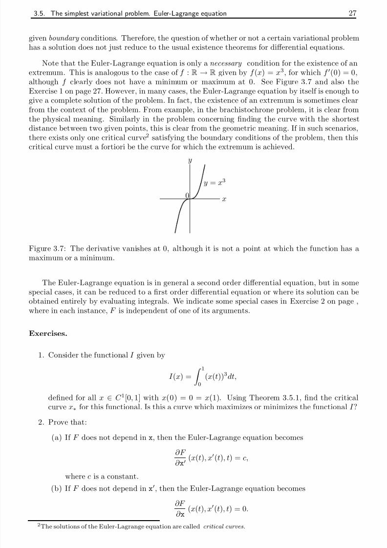
Note that the Euler-Lagrange equation is only a necessary condition for the existence of anextremum. This is analogous to the case of f : R → R given by f (x) = x3, for which f (0) = 0,although f clearly does not have a minimum or maximum at 0. See Figure 3.7 and also theExercise 1 on page 27. However, in many cases, the Euler-Lagrange equation by itself is enough togive a complete solution of the problem. In fact, the existence of an extremum is sometimes clearfrom the context of the problem. From example, in the brachistochrone problem, it is clear fromthe physical meaning. Similarly in the problem concerning finding the curve with the shortestdistance between two given points, this is clear from the geometric meaning. If in such scenarios,there exists only one critical curve2 satisfying the boundary conditions of the problem, then thiscritical curve must a fortiori be the curve for which the extremum is achieved.
x
y = x3
y
0
Figure 3.7: The derivative vanishes at 0, although it is not a point at which the function has amaximum or a minimum.
The Euler-Lagrange equation is in general a second order differential equation, but in somespecial cases, it can be reduced to a first order differential equation or where its solution can beobtained entirely by evaluating integrals. We indicate some special cases in Exercise 2 on page ,where in each instance, F is independent of one of its arguments.
Exercises.
1. Consider the functional I given by
I (x) = 1
0
(x(t))3dt,
defined for all x ∈ C 1[0, 1] with x(0) = 0 = x(1). Using Theorem 3.5.1, find the criticalcurve x∗ for this functional. Is this a curve which maximizes or minimizes the functional I ?
2. Prove that:
(a) If F does not depend in x, then the Euler-Lagrange equation becomes
∂F
∂ x(x(t), x(t), t) = c,
where c is a constant.(b) If F does not depend in x, then the Euler-Lagrange equation becomes

7/27/2019 Calculus of Variations & Optimal Control - Sasane
http://slidepdf.com/reader/full/calculus-of-variations-optimal-control-sasane 32/63
28 Chapter 3. Calculus of variations
(c) If F does not depend in t and if x∗ ∈ C 2[ti, tf ], then the Euler-Lagrange equationbecomes
F (x(t), x(t), t) − x(t)∂F
∂ x(x(t), x(t), t) = c,
where c is a constant.
Hint: What is ddt F (x(t), x(t), t)
−x(t) ∂F
∂ x(x(t), x(t), t)?
Example. (Brachistochrone problem, continued.) Determine the minimum value of the functional
I (y) =1√ 2g
x00
1 + (x(y))2
y
12
dy,
with x ∈ C 1[0, y0] and x(0) = 0, x(y0) = x0. Here3
F (x, x
, t) =1 + x2
t
12
is independent of x, and so the Euler-Lagrange equation becomes
d
dy
x(y)
1 + (x(y))21√
y
= 0.
Integrating with respect to y, we obtain
x(y) 1 + (x
(y))2
1
√ y= c,
where c is a constant. It can be shown that the general solution of this differential equation isgiven by
x(Θ) =1
2c2(Θ − sin Θ) + c,
y(Θ) =1
2c2(1 − cosΘ),
where c is another constant. The constants are chosen so that the curve passes through the points
(0, 0) and (x0, y0). This curve is known as a cycloid , and in fact it is the curve described by apoint P in a circle that rolls without slipping on the x axis, in such a way that P passes through(x0, y0); see Figure 3.8.
(0, 0)
(x0, y0)
x
y

7/27/2019 Calculus of Variations & Optimal Control - Sasane
http://slidepdf.com/reader/full/calculus-of-variations-optimal-control-sasane 33/63
3.5. The simplest variational problem. Euler-Lagrange equation 29
Example. Among all the curves joining two given points (x0, y0) and (x1, y1), find the one whichgenerates the surface of minimum area when rotated about the x axis. The area of the surface of revolution generated by rotating the curve y about the x axis is
S (y) = 2π
x1x0
y(x)
1 + (y(x))2dx.
Since the integrand does not depend explicitly on x, the Euler-Lagrange equation is
F (y(x), y(x), x) − y(x)∂F
∂ y(y(x), y(x), x) = c,
where c is a constant, that is,
y
1 + (y)2 − y(y)2
1 + (y)2= c.
Thus y = c
1 + (y)2, and it can be shown that this differential equation has the general solution
y(x) = c cosh
x + c1c
. (3.11)
This curve is called a catenary . The values of the arbitrary constants c and c1 are determinedby the conditions y(x0) = y0 and y(x1) = y1. It can be shown that the following three cases arepossible, depending on the positions of the points (x0, y0) and (x1, y1):
1. If a single curve of the form (3.11) passes through the points (x0, y0) and (x1, y1), then thiscurve is the solution of the problem; see Figure 3.9.
x0 x1
y0
y1
Figure 3.9: The catenary through (x0, y0) and (x1, y1).
2. If two critical curves can be drawn through the points (x0, y0) and (x1, y1), then one of thecurves actually corresponds to the surface of revolution if minimum area, and the other doesnot.
3. If there does not exist a curve of the form (3.11) passing through the points (x0, y0) and(x1, y1), then there is no surface in the class of smooth surfaces of revolution which achievesthe minimum area. In fact, if the location of the two points is such that the distance betweenthem is sufficiently large compared to their distances from the x axis, then the area of thesurface consisting of two circles of radius y0 and y1 will be less than the area of any surface of
revolution generated by a smooth curve passing through the points; see Figure 3.10. This isintuitively expected: imagine a soap bubble between concentric rings which are being pulled
I i ll b bbl b h i b if h di i h

7/27/2019 Calculus of Variations & Optimal Control - Sasane
http://slidepdf.com/reader/full/calculus-of-variations-optimal-control-sasane 34/63

7/27/2019 Calculus of Variations & Optimal Control - Sasane
http://slidepdf.com/reader/full/calculus-of-variations-optimal-control-sasane 35/63
3.6. Free boundary conditions 31
3.6 Free boundary conditions
Besides the simplest variational problem considered in the previous section, we now consider thevariational problem with free boundary conditions (see Figure 3.11):
LetF
(x, x, t
) be a function with continuous first and second partial derivatives with respect to(x, x, t). Then find x ∈ C 1[ti, tf ] which is an extremum for the functional
I (x) =
tf ti
F
x(t),
dx
dt(t), t
dt. (3.13)
ti tf t
Figure 3.11: Free boundary conditions.
Theorem 3.6.1 Let I be a functional of the form
I (x) =
tf ti
F
x(t),
dx
dt(t), t
dt,
where F (x, x, t) is a function with continuous first and second partial derivatives with respect to(x, x, t) and x ∈ C 1[ti, tf ]. If I has an extremum at x∗, then x∗ satisfies the Euler-Lagrange equation:
∂F
∂ x
x∗(t),
dx∗
dt(t), t
− d
dt
∂F
∂ x
x∗(t),
dx∗
dt(t), t
= 0, t ∈ [ti, tf ], (3.14)
together with the transversality conditions
∂F ∂ x
x∗(t), dx∗
dt(t), t
t=ti
= 0 and ∂F ∂ x
x∗(t), dx∗
dt(t), t
t=tf
= 0. (3.15)
Proof
Step 1. We take X = C 1[ti, tf ] and compute I (x∗). Proceeding as in the proof of Theorem 3.5.1,it is easy to see that
(I (x∗))(h) =
tf ti
∂F
∂ x(x∗(t), x∗(t), t) h(t) +
∂F
∂ x(x∗(t), x∗(t), t) h(t)
dt,
h ∈ C 1[ti, tf ]. Theorem 3.4.2 implies that this linear functional must be the zero map, that is,(I (x∗))(h) = 0 for all h ∈ C 1[ti, tf ]. In particular, it is also zero for all h in C 1[ti, tf ] such that

7/27/2019 Calculus of Variations & Optimal Control - Sasane
http://slidepdf.com/reader/full/calculus-of-variations-optimal-control-sasane 36/63
32 Chapter 3. Calculus of variations
for all h in C 1[ti, tf ] such that h(ti) = h(tf ) = 0, then this implies that he Euler-Lagrange equation(3.14) holds.
Step 2. Integration by parts in (3.16) now gives
(I (x∗))(h) = tf
ti
∂F
∂ x
(x∗(t), x∗(t), t)
−
d
dt
∂F
∂ x
(x∗(t), x∗(t), t)h(t)dt + (3.17)
∂F
∂ x(x∗(t), x∗(t), t) h(t)
t=tf
t=ti
= 0 +∂F
∂ x(x∗(t), x∗(t), t)
t=tf
h(tf ) − ∂F
∂ x(x∗(t), x∗(t), t)
t=ti
h(ti).
The integral in (3.17) vanishes since we have shown in Step 1 above that (3.14) holds. Thus thecondition I (x∗) = 0 now takes the form
∂F
∂ x(x∗(t), x∗(t), t)
t=tf
h(tf ) − ∂F
∂ x(x∗(t), x∗(t), t)
t=ti
h(ti) = 0,
from which (3.15) follows, since h is arbitrary. This completes the proof.
Exercises.
1. Find all curves y = y(x) which have minimum length between the lines x = 0 and the linex = 1.
2. Find critical curves for the following functional, when the values of x are free at the endpoints:
I (x) = 10
12
(x(t))2 + x(t)x(t) + x(t) + x(t)
dt.
Similarly, we can also consider the mixed case (see Figure 3.12), when one end of the curve isfixed, say x(ti) = xi, and the other end is free. Then it can be shown that the curve x satisfiesthe Euler-Lagrange equation, the transversality condition
∂F
∂ x(x∗(t), x∗(t), t)
t=ti
h(ti) = 0
at the free end point, and x(ti) = xi serves as the other boundary condition.
We can summarize the results by the following: critical curves for (3.13) satisfy the Euler-Lagrange equation (3.14) and moreover there holds
∂F
∂ x(x∗(t), x∗(t), t) = 0 at the free end point.
Exercises.
1. Find the curve y = y(x) which has minimum length between (0, 0) and the line x = 1.
2. Find critical curves for the following functionals:
( ) I( ) π
2
( (t))2 ( (t))2
dt (0) 0 dπ
i f

7/27/2019 Calculus of Variations & Optimal Control - Sasane
http://slidepdf.com/reader/full/calculus-of-variations-optimal-control-sasane 37/63
3.7. Generalization 33
ti titf tf
xi
xf
tt
Figure 3.12: Mixed cases.
3.7 Generalization
The results in this chapter can be generalized to the case when the integrand F is a function of more than one independent variable: if we wish to find extremum values of the functional
I (x1, . . . , xn) =
tf ti
F
x1(t), . . . , xn(t),
dx1
dt(t), . . . ,
dxn
dt(t), t
dt,
where F (x1, . . . ,xn, x1, . . . ,xn, t) is a function with continuous partial derivatives of order ≤ 2,and x1, . . . , xn are independent functions of the variable t, then following a similar analysis asbefore, we obtain n Euler-Lagrange equations to be satisfied by the optimal curve, that is,
∂F ∂ xk
(x1∗(t), . . . , xn∗(t), x1∗(t), . . . , xn∗(t), t)− ddt
∂F ∂ xk
(x1∗(t), . . . , xn∗(t), x1∗(t), . . . , xn∗(t), t)
= 0,
for t ∈ [ti, tf ], k ∈ {1, . . . , n}. Also at any end point where xk is free,
∂F
∂ xk
x1∗(t), . . . , xn∗(t),
dx1∗
dt(t), . . . ,
dxn∗
dt(t), t
= 0.
Exercise. Find critical curves of the functional
I (x1, x2) =
π2
0
(x1(t))2 + (x2(t))2 + 2x1(t)x2(t)
dt
such that x1(0) = 0, x1
π2
= 1, x2(0) = 0, x2
π2
= 1.
Remark. Note that with the above result, we can also solve the problem of finding extremalcurves for a functional of the type
I (x) : tf
ti
F x(t),dx
dt
(t), . . . ,dnx
dtn
(t), t dt,
for over all (sufficiently differentiable) curves x defined on an interval [ti tf ] taking values in R

7/27/2019 Calculus of Variations & Optimal Control - Sasane
http://slidepdf.com/reader/full/calculus-of-variations-optimal-control-sasane 38/63
34 Chapter 3. Calculus of variations
and consider the problem of finding extremal curves for the new functional I defined by
I (x1, . . . , xn) =
tf ti
F (x1(t), x2(t), . . . , xn(t), t)dt.
Using the result mentioned in this section, we can then solve this problem. Note that we eliminatedhigh order derivatives at the price of converting the scalar function into a vector -valued function.Since we can always do this, this is one of the reasons in fact for considering functionals of thetype (3.2) where no high order derivatives occur.
7/27/2019 Calculus of Variations & Optimal Control - Sasane
http://slidepdf.com/reader/full/calculus-of-variations-optimal-control-sasane 39/63
Chapter 4
Optimal control
4.1 The simplest optimal control problem
In this section, we wish to find the functions u that give extremum values of
I xi(u) =
tf ti
F (x(t), u(t), t)dt,
where x is the unique solution of the differential equation
x(t) = f (x(t), u(t)), t∈
[ti, tf ], x(ti) = xi.
We prove the following result.
Theorem 4.1.1 Let F (x, u, t) and f (x, u) be continuously differentiable functions of each of their arguments. Suppose that u∗ ∈ C [ti, tf ] is an optimal control for the functional I xi : C [ti, tf ] → R
defined as follows: If u ∈ C [ti, tf ], then
I xi(u) =
tf ti
F (x(t), u(t), t)dt,
where x(·) denotes the unique solution to the differential equation
x(t) = f (x(t), u(t)), t ∈ [ti, tf ], x(ti) = xi. (4.1)
If x∗ denotes the state corresponding to the input u∗, then there exists a p∗ ∈ C 1[ti, tf ] such that
∂F
∂ x(x∗(t), u∗(t), t) + p∗(t)
∂f
∂ x(x∗(t), u∗(t)) = − ˙ p∗(t), t ∈ [ti, tf ], p∗(tf ) = 0, (4.2)
∂F
∂ u(x∗(t), u∗(t), t) + p∗(t)
∂f
∂ u(x∗(t), u∗(t)) = 0, t ∈ [ti, tf ]. (4.3)
Proof The proof can be divided into three main steps.

7/27/2019 Calculus of Variations & Optimal Control - Sasane
http://slidepdf.com/reader/full/calculus-of-variations-optimal-control-sasane 40/63
36 Chapter 4. Optimal control
that the derivative must vanish at extremal points (now simply for a function from R to R!), weobtain a certain condition, given by equation (4.6).
Let ξ 2 ∈ C [ti, tf ] be such that ξ 2(ti) = ξ 2(tf ) = 0. Define u(t) = u∗(t) + ξ 2(t), ∈ R. Thenfrom Theorem 1.2.2, for all such that || < δ , with δ small enough, there exists a unique x(·)satisfying
x(t) = f (x(t), u(t)), t∈
[ti, tf ], x(ti) = xi. (4.4)
Define ξ 1 ∈ C 1[ti, tf ] by
ξ 1(t) =
x(t)−x∗(t)
if = 0,
0 if = 0.
Then ξ 1(ti) = 0, and x(t) = x∗(t) + ξ 1(t) for all ∈ (−δ, δ ). Let
I ξ2() =
tf ti
F (x(t), u(t), t)dt =
tf ti
F (x∗(t) + ξ 1(t), u∗(t) + ξ 2(t), t)dt.
It thus follows that I ξ2 : (
−δ, δ )
→R is differentiable (differentiation under the integral sign can
be justified!), and from the hypothesis that u∗ is optimal for I xi , it follows that the function I ξ2has an extremum for = 0. As a consequence of the necessity of the condition that the derivative
must vanish at extremal points, there must hold thatdI ξ2d
(0) = 0. But we have
dI ξ2d
() =
tf ti
∂F
∂ x(x(t), u(t), t)ξ 1(t) +
∂F
∂ u(x(t), u(t), t)ξ 2(t)
dt,
and so we obtain
tf
ti
∂F
∂ x(x∗(t), u∗(t), t)ξ 1(t) +
∂F
∂ u(x∗(t), u∗(t), t)ξ 2(t) dt = 0. (4.5)
Differentiating (4.4) with respect to , we get
∂f
∂ x(x(t), u(t))ξ 1(t) +
∂f
∂ u(x(t), u(t))ξ 2(t) − ξ 1(t) = 0.
In particular, with = 0,
∂f
∂ x(x∗(t), u∗(t))ξ 1(t) +
∂f
∂ u(x∗(t), u∗(t))ξ 2(t) − ξ 1(t) = 0. (4.6)
Step 2. We now introduce an function p in order to rewrite (4.6) in a different manner, whichwill eventually help us to conclude (4.2) and (4.3).
Let p ∈ C 1[ti, tf ] be an unspecified function. Multiplying (4.6) by p, we have that for allt ∈ [ti, tf ], there holds
p(t)
∂f
∂ x(x∗(t), u∗(t))ξ 1(t) +
∂f
∂ u(x∗(t), u∗(t))ξ 2(t) − ξ 1(t)
= 0. (4.7)
Thus adding the left hand side of (4.7) to the integrand in (4.5) does not change the integral.
Consequently, tf ∂F ∂f

7/27/2019 Calculus of Variations & Optimal Control - Sasane
http://slidepdf.com/reader/full/calculus-of-variations-optimal-control-sasane 41/63
4.1. The simplest optimal control problem 37
Hence tf ti
∂F
∂ x(x∗(t), u∗(t), t) + p(t)
∂f
∂ x(x∗(t), u∗(t)) + ˙ p(t)
ξ 1(t)+
∂F
∂ u(x∗(t), u∗(t), t) + p(t)
∂f
∂ u(x∗(t), u∗(t))
ξ 2(t)
dt + p(t)ξ 1(t)
t=tf
t=ti= 0. (4.8)
Step 3. In this final step, we choose the ‘right p’: one which makes the first summand in theintegrand appearing in (4.8) vanish (in other other words a solution of the differential equationin (4.5)) and impose a boundary condition for this special (denoted by p∗) in such a manner thatthe boundary term in (4.8) also disappears. With this choice of p, (4.8) allows one to concludethat (4.3) holds too!
Now choose p = p∗, where p∗ is such that
∂F
∂ x(x∗(t), u∗(t), t) + p∗(t)
∂f
∂ x(x∗(t), u∗(t)) + ˙ p∗(t) = 0, t
∈[ti, tf ], p∗(tf ) = 0. (4.9)
(It is easy to verify that
p∗(t) =
tf t
∂F
∂ x(x∗(s), u∗(s), s)e
R s
t
∂f ∂x
(x∗(τ ),u∗(τ ))dτ ds
satisfies (4.9).) Thus (4.8) becomes tf ti
∂F
∂ u(x∗(t), u∗(t), t) + p(t)
∂f
∂ u(x∗(t), u∗(t))
ξ 2(t)dt = 0.
Since the choice of ξ 2∈
C [ti, tf ] satisfying ξ 2(ti) = ξ 2(tf ) = 0 was arbitrary, it follows that (4.3)
holds: Indeed, if not, then the left hand side of (4.3) is nonzero (say positive) at some point in[ti, tf ], and by continuity, it is also positive in some interval [t1, t2] contained in [ti, tf ]. Set
ξ 2(t) =
(t − t1)(t2 − t) if t ∈ [t1, t2],
0 if t ∈ [t1, t2].
Then ξ 2 ∈ C [ti, tf ] and ξ 2(ti) = ξ 2(tf ) = 0. However, tf ti
∂F
∂ u(x∗(t), u∗(t), t) + p(t)
∂f
∂ u(x∗(t), u∗(t))
ξ 2(t)dt
= t2t1
∂F
∂ u (x∗(t), u∗(t), t) + p(t)∂f
∂ u (x∗(t), u∗(t))
(t − t1)(t2 − t)dt
> 0,
a contradiction. This completes the proof of the theorem.
Remarks.
1. Let X = {x ∈ C 1[ti, tf ] | x(ti) = 0} and U = C [ti, tf ]. Consider the functional I : X× U → R
defined by
I (x, u) =
tf
ti
F (x(t), u(t), t) + p∗(t)
dxdt
(t) − f (x(t), u(t))
dt.
7/27/2019 Calculus of Variations & Optimal Control - Sasane
http://slidepdf.com/reader/full/calculus-of-variations-optimal-control-sasane 42/63
38 Chapter 4. Optimal control
x∗ ∈ Rn to be an extremum of F : Rn → R subject to G : Rn → Rk is that F (x∗) = 0,where F = F + p∗ G for some p∗ ∈ Rk. The role of the Lagrange multiplier p∗ ∈ Rk, whichis vector in the finite -dimensional vector space Rk, is now played by the function p∗, whichis a vector in an infinite -dimensional vector space.
2. It should be emphasized that Theorem 4.1.1 provides a necessary condition for optimality.Thus not every u∗ that satisfies (4.2) and (4.3) for some p∗, with x∗ being the unique solutionto (4.1), needs to be optimal. (Such a u∗ satisfying is called a critical control .) However, if we already know that an optimal solution exists and that there is a unique critical control,then this critical control is obviously optimal.
4.2 The Hamiltonian and Pontryagin minimum principle
With the notation from Theorem 4.1.1, define
H (p, x, u, t) = F (x, u, t) + pf (x, u). (4.10)H is called the Hamiltonian and Theorem 4.1.1 can be equivalently be expressed in the followingform.
Theorem 4.2.1 Let F (x, u, t) and f (x, u) be continuously differentiable functions of each of their arguments. If u∗ ∈ C [ti, tf ] is an optimal control for the functional
I xi(u) =
tf ti
F (x(t), u(t), t)dt,
subject to the differential equation
x(t) = f (x(t), u(t)), t ∈ [ti, tf ], x(ti) = xi,
and if x∗ denotes the corresponding state, then there exists a p∗ ∈ C 1[ti, tf ] such that
∂H
∂ x( p∗(t), x∗(t), u∗(t), t) = − ˙ p∗(t), t ∈ [ti, tf ], p∗(tf ) = 0, and (4.11)
∂H
∂ u( p∗(t), x∗(t), u∗(t), t) = 0, t ∈ [ti, tf ]. (4.12)
Note that the differential equation x∗ = f (x∗, u∗) with x∗(ti) = xi can be expressed in termsof the Hamiltonian as follows:
∂H
∂ p( p∗(t), x∗(t), u∗(t), t) = x∗(t), t ∈ [ti, tf ], x∗(ti) = xi. (4.13)
The equations (4.11) and (4.13) resemble the equations arising in Hamiltonian mechanics, andthese equations together are said to comprise a Hamiltonian differential system . The function p∗ is called the co-state , and (4.11) is called the adjoint differential equation . This analogy withHamiltonian mechanics was responsible for the original motivation of the Pontryagin minimumprinciple, which we state below without proof.
Theorem 4.2.2 (Pontryagin minimum principle.) Let F (x, u, t) and f (x, u) be continuously dif-[ ]

7/27/2019 Calculus of Variations & Optimal Control - Sasane
http://slidepdf.com/reader/full/calculus-of-variations-optimal-control-sasane 43/63
4.2. The Hamiltonian and Pontryagin minimum principle 39
subject to the differential equation
x(t) = f (x(t), u(t)), t ∈ [ti, tf ], x(ti) = xi,
and if x∗ denotes the corresponding state, then there exists a p∗ ∈ C 1[ti, tf ] such that
∂H
∂ x ( p∗(t), x∗(t), u∗(t), t) = − ˙ p∗(t), t ∈ [ti, tf ], p∗(tf ) = 0,
and for all t ∈ [ti, tf ],
H ( p∗(t), x∗(t), u(t), t) ≥ H ( p∗(t), x∗(t), u∗(t), t) (4.14)
holds.
The fact that the optimal input u∗ minimizes the Hamiltonian (inequality (4.14)) is known asPontryagin minimum principle . Equation (4.12) is then a corollary of this result.
Exercises.
1. Find a critical control of the functional
I x0(u) =
10
(x(t))2 + (u(t))2
dt
subject to x(t) = u(t), t ∈ [0, 1], x(0) = x0.
2. Find a critical control uT ∗ and the corresponding state xT ∗ of the functional
I x0(u) =
T 0
1
2
3(x(t))2 + (u(t))2
dt
subject to x(t) = x(t) + u(t), t ∈ [0, T ], x(0) = x0. Show that there exists a constant k suchthat1
limT →∞
uT ∗(t) = k limT →∞
xT ∗(t)
for all t. What is the value of k?
Example. (Economic growth, continued.) The problem is to choose the consumption path c ∈C [0, T ] which maximizes the welfare integral
W k0(c) =
T 0
e−δtU (c(t))dt
whilst satisfying the growth equation
k(t) = Π(k(t)) − (λ + μ)k(t) − c(t), t ∈ [0, T ], k(0) = k0,
k being the capital, Π the production function, λ, μ positive constants, δ the discount factor. TheHamiltonian is given by

7/27/2019 Calculus of Variations & Optimal Control - Sasane
http://slidepdf.com/reader/full/calculus-of-variations-optimal-control-sasane 44/63
40 Chapter 4. Optimal control
From Theorem 4.2.1, it follows that any optimal control input u∗ and the corresponding state k∗satisfies
∂H
∂ c( p∗(t), k∗(t), c∗(t), t) = 0, t ∈ [0, T ],
that is,
e−δtdU
dc
(c∗(t))
− p∗(t) = 0, t
∈[0, T ]. (4.15)
The adjoint equation is
∂H
∂ x( p∗(t), k∗(t), c∗(t), t) = − ˙ p∗(t), t ∈ [0, T ], p∗(T ) = 0,
that is,
p∗(t)
dΠ
dk(k∗(t)) − (λ + μ)
= − ˙ p∗(t), t ∈ [0, T ], p∗(T ) = 0. (4.16)
From (4.15) and (4.16), we obtain
c∗(t) =
dU
dc (c∗(t))d2U dc2
(c∗(t))
dΠdk
(k∗(t)) − (λ + μ + δ )
, t ∈ [0, T ], dU dc
(c∗(T )) = 0.
So the equations governing the optimal path are the following coupled, first order, nonlineardifferential equations:
k∗(t) = Π(k(t)) − (λ + μ)k(t) − c(t), t ∈ [0, T ], k(0) = k0,
c∗(t) =dU dc
(c∗(t))d2U dc2
(c∗(t))
dΠ
dk(k∗(t)) − (λ + μ + δ )
, t ∈ [0, T ],
dU
dc(c∗(T )) = 0.
In general, it is not possible to solve these equations analytically, and instead one finds an approx-
imate solution numerically on a computer.
4.3 Generalization to vector inputs and states
In the general case when x(t) ∈ Rn and u(t) ∈ R
m, Theorem 4.2.1 holds with p∗ now being afunction taking its values in Rn:
Theorem 4.3.1 Let F (x, u, t) and f (x, u) be continuously differentiable functions of each of their arguments. If u∗ ∈ (C [ti, tf ])m is an optimal control for the functional
I xi(u) =
tf ti
F (x(t), u(t), t)dt,
subject to the differential equation
x(t) = f (x(t), u(t)), t ∈ [ti, tf ], x(ti) = xi,
and if x∗ denotes the corresponding state, then there exists a p∗ ∈ (C 1[ti, tf ])n such that
∂H ∂ x
( p∗(t), x∗(t), u∗(t), t)
= − ˙ p∗(t), t ∈ [ti, tf ], p∗(tf ) = 0, and

7/27/2019 Calculus of Variations & Optimal Control - Sasane
http://slidepdf.com/reader/full/calculus-of-variations-optimal-control-sasane 45/63
4.3. Generalization to vector inputs and states 41
Example. (Linear systems and the Riccati equation.) Let A ∈ Rn×n, B ∈ Rn×m, Q ∈ Rn×n
such that Q = Q ≥ 0 and R ∈ Rm×m such that R = R > 0. We wish to find2 optimal controlsfor the functional
I xi(u) =
tf ti
1
2
x(t)Qx(t) + u(t)Ru(t)
dt
subject to the differential equation
x(t) = Ax(t) + Bu(t), t ∈ [ti, tf ], x(ti) = xi.
The Hamiltonian is given by
H (p, x, u, t) =1
2
xQx + uRu
+ p [Ax + Bu] .
From Theorem 4.3.1, it follows that any optimal input u∗ and the corresponding state x∗ satisfies
∂H
∂ u ( p∗(t), x∗(t), u∗(t), t) = 0,
that is, u∗(t)R + p∗(t)B = 0. Thus u∗(t) = −R−1B p∗(t). The adjoint equation is
∂H
∂ x( p∗(t), x∗(t), u∗(t), t)
= − ˙ p∗(t), t ∈ [ti, tf ], p∗(tf ) = 0,
that is,
(x∗(t)Q + p∗(t)A) = − ˙ p∗(t), t ∈ [ti, tf ], p∗(tf ) = 0.
So we have
˙ p∗(t) = −A p∗(t) − Qx∗(t), t ∈ [ti, tf ], p∗(tf ) = 0.
Consequently,
d
dt
x∗(t) p∗(t)
=
A −BR−1B
−Q −A
x∗(t) p∗(t)
, t ∈ [ti, tf ], x∗(ti) = xi, p∗(tf ) = 0. (4.17)
This is a linear, time-invariant differential equation in (x∗, p∗). If we would only have to deal withinitial boundary conditions exclusively or final boundary conditions exclusively, then we couldeasily solve (4.17). However, here we have combined initial and final conditions, and so it is notclear how we could solve (4.17). It is unclear if (4.17) has a solution at all! We now prove thefollowing.
Theorem 4.3.2 Let P ∗ be a solution of the following Riccati equation
P ∗(t) = −P ∗(t)A − AP ∗(t) + P ∗(t)BR−1BP ∗(t) − Q, t ∈ [ti, tf ], P ∗(tf ) = 0.
Let x∗ be the solution of
x∗(t) = A − BR−1BP ∗(t)x∗(t), t ∈ [ti, tf ], x∗(ti) = xi,
and let
p (t) = P (t)x (t)
7/27/2019 Calculus of Variations & Optimal Control - Sasane
http://slidepdf.com/reader/full/calculus-of-variations-optimal-control-sasane 46/63
42 Chapter 4. Optimal control
Proof We have
d
dt
x∗(t) p∗(t)
=
(A − BR−1BP ∗(t))x∗(t)
P ∗(t)x∗(t) + P ∗(t)x∗(t)
=
⎡⎣
Ax∗(t) − BR−1B p∗(t)
−P ∗(t)Ax∗(t) − AP ∗(t)x∗(t) + P ∗(t)BR−1BP ∗(t)x∗(t) − Qx∗(t)+
P ∗(t)Ax∗(t) − P ∗(t)BR
−1
B
P ∗(t)x∗(t)⎤⎦
=
Ax∗(t) − BR−1B p∗(t)
−Qx∗(t) − A p∗(t)
=
A −BR−1B
−Q −A
x∗(t) p∗(t)
.
Furthermore, x∗ and p∗ satisfy x(ti) = xi and p∗(tf ) = P (tf )x∗(tf ) = 0x∗(tf ) = 0. So the pair(x∗, p∗) satisfies (4.17).
The uniqueness can be shown as follows. If (x1, p1) and (x2, p2) satisfy (4.17), then x = x1−x2,˜ p = p1
− p2 satisfy
d
dt
x(t)˜ p(t)
=
A −BR−1B
−Q −A
x(t)˜ p(t)
, t ∈ [ti, tf ], x(ti) = 0, ˜ p(tf ) = 0. (4.18)
This implies that
0 = ˜ p(tf )x(tf ) − ˜ p(ti)
x(ti)
=
tf ti
d
dt
˜ p(t)x(t)
dt
= tf
ti ˙ p(t)x(t) + ˜ p(t) ˙x(t) dt
=
tf ti
(−Qx(t) − A˜ p(t))x(t) + ˜ p(t)(Ax(t) − BR−1B˜ p(t))
dt
=
tf ti
x(t)Qx(t) + ˜ p(t)BR−1B˜ p(t)
dt.
Consequently Qx(t) = 0 and R−1B˜ p(t) = 0 for all t ∈ [ti, tf ]. From (4.18), we obtain
˙x(t) = Ax(t), t ∈ [ti, tf ], x(ti) = 0, and
˙ p(t) =
−A˜ p(t), t
∈[ti, tf ], ˜ p(tf ) = 0.
Thus x(t) = 0 and ˜ p(t) = 0 for all t ∈ [ti, tf ].
So we see that the optimal trajectories (x∗, u∗) are governed by
x∗(t) =
A − BR1−BP ∗(t)
x∗(t), t ∈ [ti, tf ], x∗(ti) = xi,
u∗(t) = −R−1BP ∗(t)x∗(t), t ∈ [ti, tf ],
where P ∗ is the solution of the Riccati equation
P ∗(t) = −P ∗(t)A − AP ∗(t) + P ∗(t)BR−1BP ∗(t) − Q, t ∈ [ti, tf ], P ∗(tf ) = 0.
Note that the optimal control has the form of a (time-varying) state-feedback law; see Figure 4.1.

7/27/2019 Calculus of Variations & Optimal Control - Sasane
http://slidepdf.com/reader/full/calculus-of-variations-optimal-control-sasane 47/63
4.4. Constraint on the state at final time. Controllability 43
plant
controller
x = Ax + Bu
u(t) = −R−1BP ∗(t)x(t)
u∗ x∗
Figure 4.1: The closed loop system.
4.4 Constraint on the state at final time. Controllability
In many optimization problems, in addition to minimizing the cost, one may also have to satisfya condition for the final state x(tf ); for instance, one may wish to drive the state to zero. Thisbrings us naturally to the notion of controllability. For the sake of simplicity, we restrict ourselvesto linear systems:
x(t) = Ax(t) + Bu(t), t ≥ ti. (4.19)
The system (4.19) is said to be controllable if for every pair of vectors xi, xf in Rn, there exists atf > ti and a control u ∈ (C [ti, tf ])
m such that the solution x of (4.19) with x(ti) = xi satisfiesx(tf ) = xf . Controllability means that any state can be driven to any other state using anappropriate control.
Example. (A controllable system.) Consider the system
x(t) = u(t),
so that
A = 0, B = 1.
Then given xi, xf ∈ R, with any tf > tf , define u ∈ C [ti, tf ] to be the constant function
u(t) =xf − xi
tf −
ti, t ∈ [ti, tf ].
By the fundamental theorem of calculus,
x(tf ) = x(ti) +
tf ti
x(τ )dτ = xi +
tf ti
u(τ )dτ = xi +xf − xi
tf − ti(tf − ti) = xf .
Note that
rank
B AB . . . An−1B (n=1)
= rank
B
= rank
1
= 1 = n,
the dimension of the state space (R).
E l (A t ll bl t ) C id th t
7/27/2019 Calculus of Variations & Optimal Control - Sasane
http://slidepdf.com/reader/full/calculus-of-variations-optimal-control-sasane 48/63
44 Chapter 4. Optimal control
so that
A =
1 00 1
, B =
10
.
The equation (4.21) implies that x2(t) = et−tix2(ti), and so if x2(ti) > 0, then x2(t) > 0 for allt ≥ ti. So a final state with the x2-component negative is never reachable by any control. Notethat
rank
B AB . . . An−1B (n=2)
= rank
B AB
= rank
1 10 0
= 1 = 2 = n,
the dimension of the state space (R2). The following theorem gives an important characterization of controllability.
Theorem 4.4.1 The system (4.19) is controllable iff rank
B AB . . . An−1B
= n, the dimension of the state space.
Exercises.
1. For what values of α is the system (4.19) controllable, if
A =
2 10 1
, B =
1α
?
2. (∗) Let A ∈ Rn×n and B ∈ R
n×1. Prove that the system (4.19) is controllable iff everymatrix commuting with A is a polynomial in A.
The following theorem tells us how we can calculate the optimal control when x(tf ) is specified,in the case of controllable linear systems.
Theorem 4.4.2 Suppose that the system
x(t) = Ax(t) + Bu(t), t ≥ ti
is controllable. Let F (x, u, t) be a continuously differentiable function of each of their arguments.
If u∗ ∈ (C [ti, tf ])m is an optimal control for the functional
I xi(u) =
tf ti
F (x(t), u(t), t)dt,
subject to the differential equation
x(t) = Ax(t) + Bu(t), t ∈ [ti, tf ], x(ti) = xi, x(tf )k = xf,k, k ∈ {1, . . . , r},
and if x∗ denotes the corresponding state, then there exists a p∗ ∈ (C 1[ti, tf ])n such that
∂H ∂ x
( p∗(t), x∗(t), u∗(t), t)
= − ˙ p∗(t), t ∈ [ti, tf ], p∗(tf )k = 0, k ∈ {r + 1, . . . , n}, and

7/27/2019 Calculus of Variations & Optimal Control - Sasane
http://slidepdf.com/reader/full/calculus-of-variations-optimal-control-sasane 49/63
4.4. Constraint on the state at final time. Controllability 45
We will not prove this theorem. Note that for a differential equation to have a unique solution,there should not be too few or too many initial and final conditions to be satisfied by that solution.Intuitively, one expects as many conditions as there are differential equations. In Theorem 4.4.2,we have, in total, 2n differential equations (for x∗ and p∗). We also have the right number of conditions: n + r for x∗, and n − r for p∗.
Exercises.
1. Find a critical control for the functional
I (u) =
10
(u(t))2dt
subject to x(t) = −2x(t) + u(t), t ∈ [0, 1], x(0) = 1 and x(1) = 0. Is this control unique?
2. Find a critical control for the functional
I (u) = T 0
(u(t))2dt
subject to x(t) = −ax(t) + u(t), t ∈ [0, T ], x(0) = x0 and x(T ) = 0. Find an expression forthe corresponding state. Prove that the critical control can be expressed as a state-feedbacklaw: u(t) = k(t , T , a)x(t). Find an expression for k(t , T , a).
3. Find a critical control for the functional
I (u) =
T 0
(xT − x(t))2 + (u(t))2
dt
subject to x(t) = −ax(t) + u(t), t ∈ [0, T ], x(0) = x0 and x(T ) = xT .
4. Find a critical control for the functional
I (u) =
10
1
2(u(t))2dt
subject to
x1(t) = x2(t),
x2(t) =
−x2(t) + u(t)
t ∈ [0, 1] and
x1(0) = 1, x2(0) = 1,
x1(1) = 0, x2(1) = 0.
5. (Higher order differential equation constraint.) Find a critical control for the functional
I (u) =
T 0
1
2(u(t))2dt
subject to the second order differential equation
7/27/2019 Calculus of Variations & Optimal Control - Sasane
http://slidepdf.com/reader/full/calculus-of-variations-optimal-control-sasane 50/63
Chapter 5
Optimality principle and
Bellman’s equation
Bellman and his co-workers pioneered a different approach for solving optimal control problems.So far we have considered continuous inputs and we have established necessary conditions for theexistence of an optimal control. We now consider a larger class of control inputs, namely piecewise continuous functions, and in Theorem 5.2.1 we give sufficient conditions for the existence of anoptimal control.
5.1 The optimality principle
The underlying idea of the optimality principle is extremely simple. Roughly speaking, the opti-mality principle simply says that any part of an optimal trajectory is optimal.
We denote the class of piecewise continuous Rm valued functions on [ti, tf ] by U [ti, tf ].
Theorem 5.1.1 (Optimality principle.) Let F (x, u, t) and f (x, u) be continuously differentiable functions of each of their arguments. Let u∗ ∈ U [ti, tf ] be an optimal control for the functional
I xi(u) = tf ti
F (x(t), u(t), t)dt,
subject tox(t) = f (x(t), u(t)), t ∈ [ti, tf ], x(ti) = xi. (5.1)
Let x∗ be the corresponding optimal state. If tm ∈ [ti, tf ), then the restriction of u∗ to [tm, tf ] is an optimal control for the functional
I x∗(tm)(u) =
tf tm
F (x(t), u(t), t)dt,
subject to
x(t) = f (x(t), u(t)), t ∈ [tm, tf ], x(tm) = x∗(tm). (5.2)
Furthermore,

7/27/2019 Calculus of Variations & Optimal Control - Sasane
http://slidepdf.com/reader/full/calculus-of-variations-optimal-control-sasane 51/63
48 Chapter 5. Optimality principle and Bellman’s equation
Proof We have
I x∗(tm)(u∗) =
tf ti
F (x∗(t), u∗(t), t)dt
=
tmti
F (x∗(t), u∗(t), t)dt +
tf tm
F (x∗(t), u∗(t), t)dt. (5.4)
From Theorem 1.2.1, it follows that the solution x1 to
x(t) = f
x(t), u∗|[tm,tf ](t)
, t ∈ [tm, tf ], x(tm) = x∗(tm),
is simply the restriction of x∗ to [tm, tf ]. Thus the second term in (5.4) is the cost I x∗(tm)
u∗|[tm,tf ](t)
subject to (5.2).
Suppose that there exists a u ∈ U [ti, tf ] such that
tf
tm
F (x(t), u(t), t)dt = I x∗(tm)(u) < I x∗(tm) u∗|[tm,tf ](t) = tf
tm
F (x∗(t), u∗(t), t)dt.
where x is the solution to (5.2) corresponding to u. Define u ∈ U [ti, tf ] by
u(t) =
u∗(t) for t ∈ [ti, tm),
u(t) for t ∈ [tm, tf ],
and let x be the corresponding solution to (5.1). From Theorem 1.2.1, it follows that
x|[ti,tm] = x∗|[ti,tm].
Hence we have
I xi(u) = tf ti
F (x(t), u(t), t)dt
=
tmti
F (x(t), u(t), t)dt +
tf tm
F (x(t), u(t), t)dt
=
tmti
F (x∗(t), u∗(t), t)dt +
tf tm
F (x(t), u(t), t)dt
=
tmti
F (x∗(t), u∗(t), t)dt + I x∗(tm)(u)
< tmti F (x∗(t), u∗(t), t)dt +
˜I x∗(tm)
u∗|[tm,tf ](t)
=
tmti
F (x∗(t), u∗(t), t)dt +
tf tm
F (x∗(t), u∗(t), t)dt
= I xi(u∗),
which contradicts the optimality of u∗. This proves that an optimal control for I x∗(tm) subjectto (5.2) exists and it is given by the restriction of u∗ to [tm, tf ]. From (5.4), it follows that (5.3)holds.
Note that we have shown that
minU[ ]
I x∗(tm)(u) = I x∗(tm)
u∗|[tm,tf ](t)
.

7/27/2019 Calculus of Variations & Optimal Control - Sasane
http://slidepdf.com/reader/full/calculus-of-variations-optimal-control-sasane 52/63
5.2. Bellman’s equation 49
ti tm tf
xi
x∗(tm)
u∗|[ti,tm]
u
u∗|[tm,tf ]
Figure 5.1: Optimality principle.
5.2 Bellman’s equation
In this section we will prove Theorem 5.2.1 below, which gives a sufficient condition for the ex-
istence of an optimal control in terms of the existence of an appropriate solution to Bellman’sequation (5.6). However, we first provide a heuristic argument that leads one to Bellman’s equa-tion: we do not start by asking when the optimal control problem has a solution, but ratherwe begin by assuming that the optimal control problem is solvable and study the so-called valuefunction, which will lead us to Bellman’s equation.
Let tm ∈ [ti, tf ). Define the value function V : Rn × [ti, tf ] → R by
V (xm, tm) = minu∈U[tm,tf ]
tf tm
F (x(t), u(t), t)dt, (5.5)
where x(·) is the unique solution to
x(t) = f (x(t), u(t)), t ∈ [tm, tf ], x(tm) = xm.
With this notation, in Theorem 5.1.1, we have shown that
V (x∗(tm), tm) = minu∈U[tm,tf ]
tf tm
F (x(t), u(t), t)dt =
tf tm
F (x∗(t), u∗(t), t)dt.
Consequently
V (x∗(tm + ), tm + ) − V (x∗(tm), tm) = −
tm+
tm
F (x∗(t), u∗(t), t)dt.
It is tempting to divide by on both sides and let tend to 0. Formally, the left hand side wouldbecome
∂V
∂ t(x∗(tm), tm) +
∂V
∂ x(x∗(tm), tm)f (x∗(tm), u∗(tm)),
while the right hand side would become
−F (x∗(tm), u∗(tm), tm).
Thus we would obtain the equation
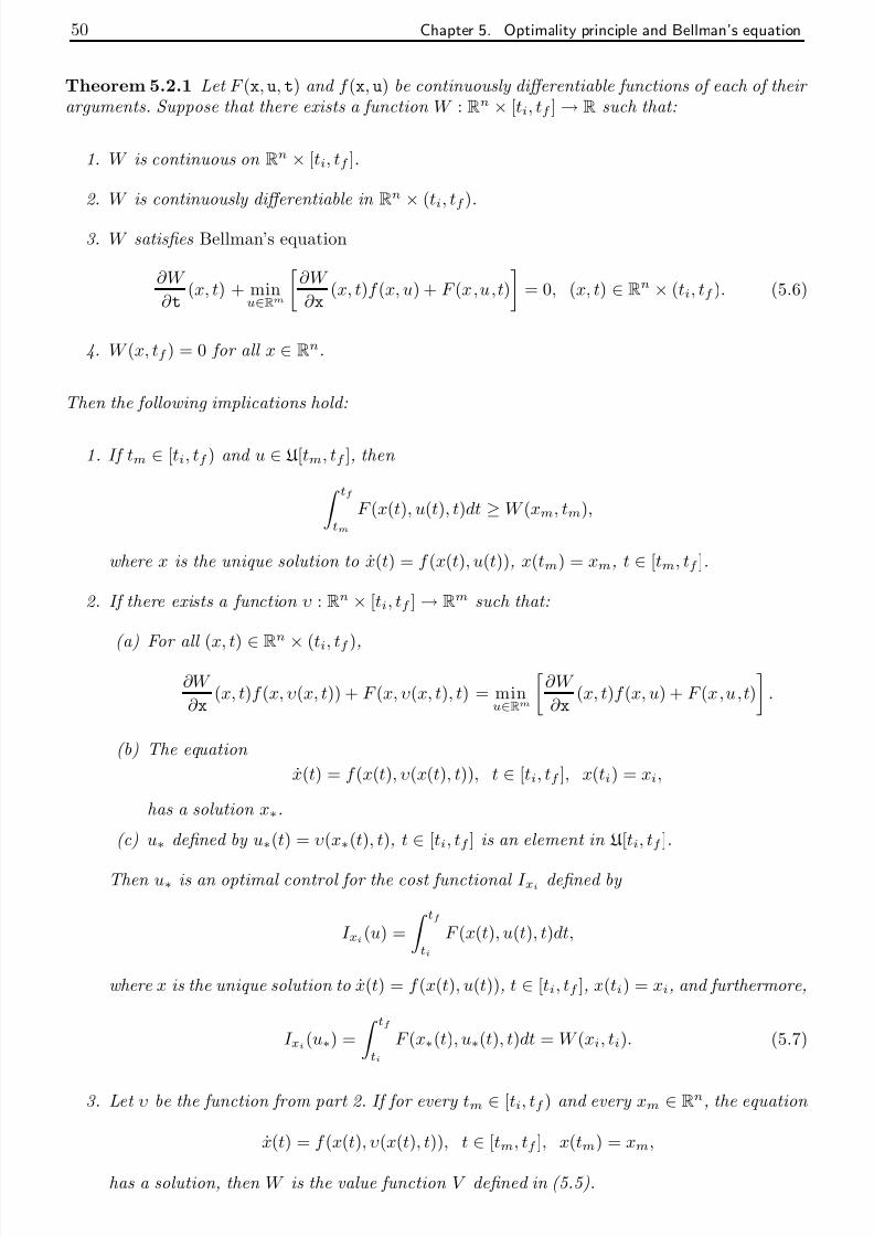
7/27/2019 Calculus of Variations & Optimal Control - Sasane
http://slidepdf.com/reader/full/calculus-of-variations-optimal-control-sasane 53/63
50 Chapter 5. Optimality principle and Bellman’s equation
Theorem 5.2.1 Let F (x, u, t) and f (x, u) be continuously differentiable functions of each of their arguments. Suppose that there exists a function W : Rn × [ti, tf ] → R such that:
1. W is continuous on Rn × [ti, tf ].
2. W is continuously differentiable in Rn
×(ti, tf ).
3. W satisfies Bellman’s equation
∂W
∂ t(x, t) + min
u∈Rm
∂W
∂ x(x, t)f (x, u) + F (x,u,t)
= 0, (x, t) ∈ Rn × (ti, tf ). (5.6)
4. W (x, tf ) = 0 for all x ∈ Rn.
Then the following implications hold:
1. If tm ∈ [ti, tf ) and u ∈ U [tm, tf ], then
tf tm
F (x(t), u(t), t)dt ≥ W (xm, tm),
where x is the unique solution to x(t) = f (x(t), u(t)), x(tm) = xm, t ∈ [tm, tf ].
2. If there exists a function υ : Rn × [ti, tf ] → Rm such that:
(a) For all (x, t) ∈Rn
× (ti, tf ),
∂W
∂ x(x, t)f (x, υ(x, t)) + F (x, υ(x, t), t) = min
u∈Rm
∂W
∂ x(x, t)f (x, u) + F (x,u,t)
.
(b) The equation
x(t) = f (x(t), υ(x(t), t)), t ∈ [ti, tf ], x(ti) = xi,
has a solution x∗.
(c) u∗ defined by u∗(t) = υ(x∗(t), t), t ∈ [ti, tf ] is an element in U [ti, tf ].
Then u∗ is an optimal control for the cost functional I xi defined by
I xi(u) =
tf ti
F (x(t), u(t), t)dt,
where x is the unique solution to x(t) = f (x(t), u(t)), t ∈ [ti, tf ], x(ti) = xi, and furthermore,
I xi(u∗) =
tf ti
F (x∗(t), u∗(t), t)dt = W (xi, ti). (5.7)
3. Let υ be the function from part 2. If for every tm ∈ [ti, tf ) and every xm ∈ Rn, the equation
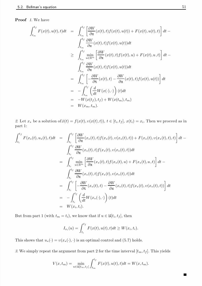
7/27/2019 Calculus of Variations & Optimal Control - Sasane
http://slidepdf.com/reader/full/calculus-of-variations-optimal-control-sasane 54/63
5.2. Bellman’s equation 51
Proof 1. We have tf tm
F (x(t), u(t), t)dt =
tf tm
∂W
∂ x(x(t), t)f (x(t), u(t)) + F (x(t), u(t), t)
dt −
tf
tm
∂W
∂ x(x(t), t)f (x(t), u(t))dt
≥
tf
tm
minu∈Rm
∂W
∂ x(x(t), t)f (x(t), u) + F (x(t), u , t)
dt −
tf tm
∂W
∂ x(x(t), t)f (x(t), u(t))dt
=
tf tm
−∂W
∂ t(x(t), t) − ∂W
∂ x(x(t), t)f (x(t), u(t))
dt
= − tf tm
d
dtW (x(·), ·)
(t)dt
= −W (x(tf ), tf ) + W (x(tm), tm)= W (xm, tm).
2 . Let x∗ be a solution of x(t) = f (x(t), υ(x(t), t)), t ∈ [ti, tf ], x(ti) = xi. Then we proceed as inpart 1:
tf ti
F (x∗(t), u∗(t), t)dt =
tf ti
∂W
∂ x(x∗(t), t)f (x∗(t), υ(x∗(t), t)) + F (x∗(t), υ(x∗(t), t), t)
dt −
tf ti
∂W
∂ x (x∗(t), t)f (x∗(t), υ(x∗(t), t))dt
=
tf ti
minu∈Rm
∂W
∂ x(x∗(t), t)f (x∗(t), u) + F (x∗(t), u , t)
dt −
tf ti
∂W
∂ x(x∗(t), t)f (x∗(t), υ(x∗(t), t))dt
=
tf ti
−∂W
∂ t(x∗(t), t) − ∂W
∂ x(x∗(t), t)f (x∗(t), υ(x∗(t), t))
dt
=−
tf
ti d
dtW (x∗(
·),
·) (t)dt
= W (xi, ti).
But from part 1 (with tm = ti), we know that if u ∈ U [ti, tf ], then
I xi(u) =
tf ti
F (x(t), u(t), t)dt ≥ W (xi, ti).
This shows that u∗(·) = υ(x∗(·), ·) is an optimal control and (5.7) holds.
3 . We simply repeat the argument from part 2 for the time interval [ tm, tf ]. This yields
t

7/27/2019 Calculus of Variations & Optimal Control - Sasane
http://slidepdf.com/reader/full/calculus-of-variations-optimal-control-sasane 55/63
52 Chapter 5. Optimality principle and Bellman’s equation
In the following example, we show how Theorem 5.2.1 can be used to calculate an optimalcontrol.
Example. Consider the following linear system with state space R:
x(t) = u(t), t
∈[0, 1], x(0) = x0,
with cost criterion
I x0(u) =
10
(x(t))2 + (u(t))2
dt.
For this system, Bellman’s equation is given by
∂W
∂ t(x, t) + min
u∈R
∂W
∂ x(x, t)u + x2 + u2
= 0, (x, t) ∈ R× (0, 1), W (x, 1) = 0.
It is easy to see that the minimum in the above is assumed for
u = υ(x, t) = −12 ∂W ∂ x
(x, t).
Thus we obtain
∂W
∂ t(x, t) + x2 − 1
4
∂W
∂ x(x, t)
2
= 0, (x, t) ∈ R× (0, 1), W (x, 1) = 0.
This is a nonlinear partial differential equation. It is easy to see that if (x∗, u∗) is an optimaltrajectory with initial state x0, then for every λ ∈ R, (λx∗, λu∗) is an optimal trajectory withrespect to the initial state λx0. Therefore the value function is quadratic in x: W (λx, t) =λ2W (x, t). In particular,
W (x, t) = x2W (1, t) = x2 p∗(t),
where p∗(t) := W (1, t). Consequently,
x2 ˙ p∗(t) + x2 − 1
4(2x)2( p∗(t))2 = 0, (x, t) ∈ R× (0, 1), p∗(1) = 0.
Dividing by x2, we obtain the Riccati equation
˙ p∗(t) = ( p∗(t))2 − 1, t ∈ (0, 1), p∗(1) = 0.
This has the solution
p∗(t) = e−t+1
− et−1
e−t+1 + et−1.
(See the exercise on page 3.) Thus
W (x, t) = x2 e−t+1 − et−1
e−t+1 + et−1.
Also the linear time varying differential equation
x(t) = υ(x(t), t) = −x(t) p∗(t), t ∈ [0, 1], x(0) = x0
has the solution x∗(t) = x0e−R t0 p∗(τ )dτ . (5.8)

7/27/2019 Calculus of Variations & Optimal Control - Sasane
http://slidepdf.com/reader/full/calculus-of-variations-optimal-control-sasane 56/63
5.2. Bellman’s equation 53
where x∗ is the optimal state given by (5.8). Note that the optimal control is given in the form of a (time-varying) state feedback. The value function is given by V (x, t) = x2 p∗(t).
Exercise.
Its good to keep in mind that not every optimal control problem is solvable. Prove that for
the following problem, there is no minimizing input u ∈ U [ti, tf ]:
x(t) = u(t), t ∈ [0, 1], x(0) = 1,
with the cost function I x0(u) = 10
(x(t))2dt.
7/27/2019 Calculus of Variations & Optimal Control - Sasane
http://slidepdf.com/reader/full/calculus-of-variations-optimal-control-sasane 57/63
Bibliography
[1] R.W. Brockett. Finite Dimensional Linear Systems . John Wiley, 1970.
[2] D.N. Burghes and A. Graham. Introduction to Control Theory, Including Optimal Control .John Wiley, 1980.
[3] I.M. Gelfand and S.V. Fomin. Calculus of Variations . Dover, 1963.
[4] H.J. Sussmann and J.C. Willems. 300 years of optimal control: from the brachystochroneproblem to the maximum principle. IEEE Control Systems , 17:32–44, 1997.
[5] J.L. Troutman. Variational Calculus and Optimal Control: Optimization with Elementary Convexity . 2nd Edition, Springer, 1996.
[6] R. Weinstock. Calculus of Variations with applications to physics and engineering . Dover,1974.
[7] H.J. Zwart. Optimal Control Theory . Rijksuniversiteit Groningen, 1997.

7/27/2019 Calculus of Variations & Optimal Control - Sasane
http://slidepdf.com/reader/full/calculus-of-variations-optimal-control-sasane 58/63
Index
C [ti, tf ], 19C 1[ti, tf ], 19
continuous linear functional, 22
adjoint differential equation, 38admissible functions, 21affine linear map, 21
arc length, 21arc length, 16
Bellman’s equation, 50brachistochrone problem, 16
calculus of variations, 15catenary, 29Cauchy’s problem, 26closed loop system, 43co-state, 38
commuting matrices, 6conservation of energy, 16constrained optimization problem, 37continuous functional, 20control, 1control system, 2control theory, 1controllability, 43critical control, 38critical curve, 27
cycloid, 28
dense set, 6diagonalizable matrix, 6discount rate, 10distance, 19
economic growth, 9economic growth, 14, 39Euler, 17Euler-Lagrange equation, 24, 31
exploited population, 11
F h´ d i i 22
fundamental theorem of calculus, 43
Hamiltonian, 38Hamiltonian mechanics, 38Hamiltonian differential system, 38
input, 2
Johann Bernoulli, 16
kernel, 19
Lagrange multiplier, 38Lagrange multiplier theorem, 37length of a curve, 12linear control system, 2linear functional, 18linear quadratic control problem, 41linear space, 18
linear span, 19linear system, 41Lipschitz condition, 2local extremum, 23LQ problem, 41
method of finite differences, 17metric space, 19mixed boundary conditions, 32
norm, 19normed linear space, 19
optimal control, 13optimal control theory, 4optimal state, 13optimal trajectory, 13optimality principle, 47
path independence, 13piecewise continuous, 2
Pontryagin minimum principle, 39present value, 11
7/27/2019 Calculus of Variations & Optimal Control - Sasane
http://slidepdf.com/reader/full/calculus-of-variations-optimal-control-sasane 59/63
58 Index
relative stationarity condition, 37Riccati equation, 3, 41, 52
state, 2state equation, 2state feedback, 53
state-feedback, 42, 45static state-feedback, 39system, 1
Taylor’s theorem, 25transversality conditions, 31triangle inequality, 19
underdetermined differential equation, 1utility function, 10
value function, 49vector space, 18vector-valued function, 4Verhulst model, 11
welfare integral, 10
zero element, 18
7/27/2019 Calculus of Variations & Optimal Control - Sasane
http://slidepdf.com/reader/full/calculus-of-variations-optimal-control-sasane 60/63
Mock examination
MA305
Control Theory(Half Unit)
Suitable for all candidates
Instructions to candidates
Time allowed: 2 hours
This examination paper contains 6 questions. You may attempt as many questions as you wish,
but only your best 4 questions will count towards the final mark. All questions carry equal
numbers of marks.
Please write your answers in dark ink (preferably black or blue) only.
Calculators are not allowed in this exam.
You are supplied with: Answer Booklet
c LSE 2004 / MA305 Mock Examination Question Paper Page 1 of 4

7/27/2019 Calculus of Variations & Optimal Control - Sasane
http://slidepdf.com/reader/full/calculus-of-variations-optimal-control-sasane 61/63
1 (a) Let X be a linear space over R. Give the definition of a norm on X .
(b) If I : X →R is a functional on a normed linear space X , when is I said to be contin-
uous at x∗ ∈ X ?
(c) Is the linear functional I : C [0,1] →R defined by
I ( x) =Z
1
0
x(t )dt for x ∈C [0,1],
continuous at 0? Here the linear space C [0,1] is equipped with the usual norm
x = supt ∈[0,1]
| x(t )|.
2 (a) Regarding the left hand side of the obvious inequality
Z t f t i
( x1(t ) + rx2(t ))2dt 0
as a quadratic function of r , prove the Cauchy-Schwarz inequality: Z t f t i
( x1(t ))2dt
Z t f t i
( x2(t ))2dt
Z t f t i
x1(t ) x2(t )dt
2
for all x1, x2 ∈C [t i, t f ].
HINT: The minimum value of the quadratic function Q(r ) = Ar 2 + Br +C with
A> 0 is given by 4 AC − B2
4 A.
(b) Consider the linear functional I defined by
I ( x) =Z 10e−2t
d
dt x(t )
2
dt
for x ∈C 1[0,1] with x(0) = 0 and x(1) = 1. Using the result from part (a), show that
I ( x) 2
e2 1.
HINT: Use the Cauchy-Schwarz inequality with x1(t ) = e2t and x2 = e−2t d dt x(t ).
(c) Using the Euler-Lagrange equation, find a critical curve x∗ for I , and find I ( x∗).
Using part (b) show that x∗ indeed minimizes the functional I .
3 Consider the functional I given by
I ( x) =Z
2
0
1
2
d
dt x(t )
2
+ x(t )d
dt x(t ) +
d
dt x(t ) + x(t )
dt
defined for all x ∈C 1 [0,2].
(a) Write the Euler-Lagrange equation for this problem.
c LSE 2004 / MA305 Mock Examination Question Paper Page 2 of 4

7/27/2019 Calculus of Variations & Optimal Control - Sasane
http://slidepdf.com/reader/full/calculus-of-variations-optimal-control-sasane 62/63
(b) Write the transversality conditions at the endpoints t = 0 and t = 2.
(c) Determine the solution of the Euler-Lagrange equation found in part (a) that satisfies
the transversality conditions from part (b).
4 Consider the functional I : C [0,1] →R defined by
I (u) = Z 1
0
[3( x(t ))2 + (u(t ))2]dt (1)
where x denotes the unique solution to
d
dt x(t ) = x(t ) +u(t ), t ∈ [0,1], x(0) = 1. (2)
(a) Using the Hamiltonian method, write down the equations that govern an optimal
control for (1) subject to (2).
(b) Find an equation that describes the evolution of the state x∗ and the co-state p∗ and
specify the boundary conditions x∗(0) and p∗(1).
(c) Solve the equations from part (b) and determine a critical control.
5 (a) Consider the controllable linear system
d
dt x(t ) = Ax(t ) + Bu(t ), t t i, (3)
where A∈Rn×n and B∈Rn×m. Suppose thatQ=Q∈Rn be a positive semidefinite
matrix and let R = R ∈ Rm be a positive definite matrix. Let I : (C [t i, t f ])m → R
defined by
I (u) =Z t f t i
1
2 x(t )
Qx(t ) +u(t )
Ru(t )dt , (4)
where x is the solution to (3) on the time interval [t i, t f ] with x(t i) = xi ∈ Rn and
x(t f ) = x f ∈Rn. Using the Hamiltonian theorem on optimal control, write down the
differential equations for the optimal state x∗ and the co-state p∗ for I given by (4)
subject to (3).
(b) Give a necessary and sufficient condition for controllability of the system (3) in
terms of A and B.
(c) Show that if the system described by (3) is controllable, then for every λ that is an
eigenvalue of A with eigenvector v, there holds that Bv 6= 0.
6 Consider the cost functional I :C [0,1] →R defined by
I (u) =Z
1
0
[3( x(t ))2 + (u(t ))2]dt (5)
where x denotes the unique solution to
d
dt x(t ) = x(t ) +u(t ), t ∈ [0,1], x(0) = 1. (6)
c LSE 2004 / MA305 Mock Examination Question Paper Page 3 of 4

7/27/2019 Calculus of Variations & Optimal Control - Sasane
http://slidepdf.com/reader/full/calculus-of-variations-optimal-control-sasane 63/63
(a) Write Bellman’s equation associated with the above functional.
(b) Assuming that the solution W to Bellman’s equation in part (a) is quadratic in x:
W ( x, t ) = x2W (1, t ), find a solution W to Bellman’s equation.
(c) Find the optimal state x∗ and the optimal control u∗ for I given by (5) subject to (6).