Calculus of variations in image processing

Jean-François Aujol

CMLA, ENS Cachan, CNRS, UniverSud,

61 Avenue du Président Wilson, F-94230 Cachan, FRANCE

Email : Jean-Francois.Aujol@cmla.ens-cachan.fr

http://www.cmla.ens-cachan.fr/membres/aujol.html

18 september 2008

Note: This document is a working and uncomplete version, subject to errors and changes. Readers

are invited to point out mistakes by email to the author.

This document is intended as course notes for second year master students. The author encourage

the reader to check the references given in this manuscript. In particular, it is recommended to look at

[9] which is closely related to the subject of this course.

Contents

1. Inverse problems in image processing 41.1 Introduction . . . . . . . . . . . . . . . . . . . . . . . . . . . . . . . . . . . . . . 41.2 Examples . . . . . . . . . . . . . . . . . . . . . . . . . . . . . . . . . . . . . . . 41.3 Ill-posed problems . . . . . . . . . . . . . . . . . . . . . . . . . . . . . . . . . . . 61.4 An illustrative example . . . . . . . . . . . . . . . . . . . . . . . . . . . . . . . . 81.5 Modelization and estimator . . . . . . . . . . . . . . . . . . . . . . . . . . . . . 10

1.5.1 Maximum Likelihood estimator . . . . . . . . . . . . . . . . . . . . . . . 101.5.2 MAP estimator . . . . . . . . . . . . . . . . . . . . . . . . . . . . . . . . 11

1.6 Energy method and regularization . . . . . . . . . . . . . . . . . . . . . . . . . . 11

2. Mathematical tools and modelization 142.1 Minimizing in a Banach space . . . . . . . . . . . . . . . . . . . . . . . . . . . . 142.2 Banach spaces . . . . . . . . . . . . . . . . . . . . . . . . . . . . . . . . . . . . . 14

2.2.1 Preliminaries . . . . . . . . . . . . . . . . . . . . . . . . . . . . . . . . . 142.2.2 Topologies in Banach spaces . . . . . . . . . . . . . . . . . . . . . . . . . 172.2.3 Convexity and lower semicontinuity . . . . . . . . . . . . . . . . . . . . . 192.2.4 Convex analysis . . . . . . . . . . . . . . . . . . . . . . . . . . . . . . . . 23

2.3 Subgradient of a convex function . . . . . . . . . . . . . . . . . . . . . . . . . . 232.4 Legendre-Fenchel transform: . . . . . . . . . . . . . . . . . . . . . . . . . . . . . 242.5 The space of funtions with bounded variation . . . . . . . . . . . . . . . . . . . 26

2.5.1 Introduction . . . . . . . . . . . . . . . . . . . . . . . . . . . . . . . . . . 262.5.2 Definition . . . . . . . . . . . . . . . . . . . . . . . . . . . . . . . . . . . 272.5.3 Properties . . . . . . . . . . . . . . . . . . . . . . . . . . . . . . . . . . . 282.5.4 Decomposability of BV (Ω): . . . . . . . . . . . . . . . . . . . . . . . . . 282.5.5 SBV . . . . . . . . . . . . . . . . . . . . . . . . . . . . . . . . . . . . . . 302.5.6 Sets of finite perimeter . . . . . . . . . . . . . . . . . . . . . . . . . . . . 322.5.7 Coarea formula and applications . . . . . . . . . . . . . . . . . . . . . . . 33

3. Energy methods 353.1 Introduction . . . . . . . . . . . . . . . . . . . . . . . . . . . . . . . . . . . . . . 353.2 Tychonov regularization . . . . . . . . . . . . . . . . . . . . . . . . . . . . . . . 35

3.2.1 Introduction . . . . . . . . . . . . . . . . . . . . . . . . . . . . . . . . . . 353.2.2 Sketch of the proof (to fix some ideas) . . . . . . . . . . . . . . . . . . . 363.2.3 General case . . . . . . . . . . . . . . . . . . . . . . . . . . . . . . . . . . 363.2.4 Minimization algorithms . . . . . . . . . . . . . . . . . . . . . . . . . . . 39

3.3 Rudin-Osher-Fatemi model . . . . . . . . . . . . . . . . . . . . . . . . . . . . . . 403.3.1 Introduction . . . . . . . . . . . . . . . . . . . . . . . . . . . . . . . . . . 403.3.2 Interpretation as a projection . . . . . . . . . . . . . . . . . . . . . . . . 453.3.3 Euler-Lagrange equation for (3.67): . . . . . . . . . . . . . . . . . . . . . 473.3.4 Other regularization choices . . . . . . . . . . . . . . . . . . . . . . . . . 483.3.5 Half quadratic minimmization . . . . . . . . . . . . . . . . . . . . . . . . 50

3.4 Wavelets . . . . . . . . . . . . . . . . . . . . . . . . . . . . . . . . . . . . . . . . 533.4.1 Besov spaces . . . . . . . . . . . . . . . . . . . . . . . . . . . . . . . . . . 53

2

3.4.2 Wavelet shrinkage . . . . . . . . . . . . . . . . . . . . . . . . . . . . . . . 543.4.3 Variational interpretation . . . . . . . . . . . . . . . . . . . . . . . . . . 55

4. Advanced topics: Image decomposition 564.1 Introduction . . . . . . . . . . . . . . . . . . . . . . . . . . . . . . . . . . . . . . 564.2 A space for modeling oscillating patterns in bounded domains . . . . . . . . . . 57

4.2.1 Definition and properties . . . . . . . . . . . . . . . . . . . . . . . . . . . 574.2.2 Study of Meyer problem . . . . . . . . . . . . . . . . . . . . . . . . . . . 60

4.3 Decomposition models and algorithms . . . . . . . . . . . . . . . . . . . . . . . 614.3.1 Which space to use? . . . . . . . . . . . . . . . . . . . . . . . . . . . . . 614.3.2 Parameter tuning . . . . . . . . . . . . . . . . . . . . . . . . . . . . . . . 624.3.3 TV −G algorithms . . . . . . . . . . . . . . . . . . . . . . . . . . . . . . 644.3.4 TV − L1 . . . . . . . . . . . . . . . . . . . . . . . . . . . . . . . . . . . . 654.3.5 TV −H−1 . . . . . . . . . . . . . . . . . . . . . . . . . . . . . . . . . . . 664.3.6 TV -Hilbert . . . . . . . . . . . . . . . . . . . . . . . . . . . . . . . . . . 674.3.7 Using negative Besov space . . . . . . . . . . . . . . . . . . . . . . . . . 684.3.8 Using Meyer’s E space . . . . . . . . . . . . . . . . . . . . . . . . . . . . 694.3.9 Applications of image decomposition . . . . . . . . . . . . . . . . . . . . 71

A. Discretization 71

3

1. Inverse problems in image processing

For this section, we refer the interested reader to [71]. We encourage the reader not familiarwith matrix to look at [29].

1.1 Introduction

In many problems in image processing, the goal is to recover an ideal image u from an obser-vation f .

u is a perfect original image describing a real scene.f is an observed image, which is a degraded version of u.The degradation can be due to:

• Signal transmission: there can be some noise (random perturbation).

• Defects of the imaging system: there can be some blur (deterministic perturbation).

The simplest modelization is the following:

f = Au+ v (1.1)

where v is the noise, and A is the blur, a linear operator (for example a convolution).The following assumptions are classical:

• A is known (but often not invertible)

• Only some statistics (mean, variance, . . . ) are know of n.

1.2 Examples

Image restoration (Figure 1)f = u+ v (1.2)

with n a white gaussian noise with standard deviation σ.

Radar image restoration (Figure 2)

f = uv (1.3)

with v a gamma noise with mean one.Poisson distribution for tomography.

Image decomposition (Figure 3)f = u+ v (1.4)

u is the geometrical component of the original image f (u can be seen a s a sketch of f),and v is the textured component of the original image f (v contains all the details of f).

4

Original image Noisy image f (σ = 30) Restoration (u)

Figure 1: Denoising

Noise free image Speckled image (f) restored image u

Figure 2: Denoising of a synthetic image with gamma noise. f has been corrupted by somemultiplicative noise with gamma law of mean one.

Original image (f) = BV component (u) + Oscillatory component(v)

Figure 3: Image decomposition

5

Original image Degraded image Restored image

Figure 4: Example of TV deconvolution

Degraded image Inpainted image

Figure 5:

Image deconvolution (Figure 4)f = Au+ v (1.5)

Image inpainting [56] (Figure 5)

Zoom [54] (Figure 6)

1.3 Ill-posed problems

Let X and Y be two Hilbert spaces. Let A : X → Y a continous linear application (in short,an operator).

Consider the following problem:

Given f ∈ Y, find u ∈ X such that f = Au (1.6)

The problem is said to be well-posed if

(i) ∀f ∈ Y there exists a unique u ∈ X such that f = Au.

(ii) The solution u depends continuously on f .

6

Figure 6: Top left: ideal image; top right: zoom with total variation minimization; bottom left:zoom by pixel duplication; bottom right: zoom with cubic splines

7

In other words, the problem is well-posed if A is invertible and its inverse A−1 : Y → X iscontinuous.

Conditions (i) and (ii) are referred to as the Hadamard conditions.A problem that is not well-posed is said to be ill-posed.Notice that a mathematically well-posed problem may be ill-posed in practice: the solution

may exist, be unique, and depend continuously on the data, but still be very sensitive to smallperturbations of it. An eror δf produces the error δu = A−1δf , which may have dramaticconsequences on the interpretation of the solution. In particular, if ‖A−1‖ is very large, errorsmay be strongly amplified by the action of A−1. There can also be some computational timeissues.

1.4 An illustrative example

See [29] for the defintion of ‖.‖2 of a vector, a matrix, a positive symmetric matrix, an orthogonalmatrix, . . .

We consider the following problem:

f = Au+ v (1.7)

‖v‖ is the the amount of noise.We assume that A is a real symetric positive matrix, and has some small eigenvalues. ‖A−1‖

is thus very large. We want to compute a solution by filtering.Since A is symetric, there exists an orthogonal matrix P (i.e. P−1 = P T ) such that:

A = PDP T (1.8)

with D = diag(λi) a diagonal matrix, and λi > 0 for all i.We have:

A−1f = u+ A−1v = u+ PD−1P Tv (1.9)

with D−1 = diag(λ−1i ). It is easy to see that instabilities arise from small eigenvalues λi.

Regularization by filtering: One way to overcome this problem consists in modifying theλ−1

i : we multiply them by wα(λ2i ). wα is chosen such that:

wα(λ2)λ−1 → 0 when λ→ 0. (1.10)

This filters out singular components from A−1f and leads to an approximation to u by uα

defined by:uα = PD−1

α P Tf (1.11)

where D−1α = diag(wα(λ2

i )λ−1i ).

To obtain some accuracy, one must retain singular components corresponding to large sin-gular values. This is done by choosing wα(λ2) ≈ 1 for large values of λ.

For wα, we may chose (truncated SVD):

wα(λ2) =

1 if λ2 > α.0 if λ2 ≤ α.

(1.12)

We may also choose a smoother function (Tychonov filter function):

wα(λ2) =λ2

λ2 + α(1.13)

An obvious question arises: can the regularization parameter α be selected to guaranteeconvergence as the error level ‖v‖ goes to zero?

8

Error analysis: We denote by Rα the regularization operator:

Rα = PD−1α P T (1.14)

We have uα = Rαf . The regularization error is given by:

eα = uα − u = RαAu− u+Rαv = etruncα + enoise

α (1.15)

where:etrunc

α = RαAu− u = P (D−1α D − Id)P Tu (1.16)

and:enoise

α = Rαv = PD−1α P Tv (1.17)

etruncα is the error due to the regularization (it quantifies the loss of information due to the

regularizing filter). enoiseα is called the noise amplification error.

We first deal with etruncα . Since wα(λ2) → 1 as α → 0, we have D−1

α → D−1 as α → 0 andthus:

etruncα → 0 as α → 0. (1.18)

To deal with the noise amplification error, we use the following inequality for λ > 0:

wα(λ2)λ−1 ≤ 1√α

(1.19)

Remind that ‖P‖ = 1 since P orthogonal. We thus deduce that:

enoiseα ≤ 1√

α‖v‖ (1.20)

where we recall that ‖v‖ = ‖v‖ is the amount of noise. To conclude, it suffice to choose α = ‖v‖p

with p < 2, and let ‖v‖ → 0: we get enoiseα → 0.

Now, if we choose α = ‖v‖p with 0 < p < 2, we have:

eα → 0 as ‖v‖ → 0. (1.21)

For such a regularization parameter choice, we say that the method is convergent.

Rate of convergence: We assume a range condition:

u = A−1z (1.22)

Since A = PDP T , we have:

etruncα = P (D−1

α D − Id)P Tu = P (D−1α −D−1)P T z (1.23)

Hence:‖etrunc

α ‖22 ≤ ‖D−1

α −D−1‖2‖z‖2 (1.24)

Since D−1α −D−1 = diag((wα(λ2

i ) − 1)λ−1i ), we deduce that:

‖etruncα ‖2

2 ≤ α‖z‖2 (1.25)

We thus get:

‖eα‖ ≤ √α‖z‖ +

1√α‖v‖ (1.26)

The right-hand side is minimized by taking α = ‖v‖/‖z‖. This yields:

‖eα‖ ≤ 2√

‖z‖‖v‖ (1.27)

Hence the convergence order of the method is 0(√

‖v‖).

9

1.5 Modelization and estimator

We consider the following additive model:

f = Au+ v (1.28)

Idea: We want to comput the most likely u with respect to the observation f . Naturalprobabilistic quantities: P (F |U), and P (u|F ).

1.5.1 Maximum Likelihood estimator

Let us assume that the noise v follows a Gaussian law with zero mean:

P (V = v) =1√

2πσ2exp

(

−(v)2

2σ2

)

(1.29)

We have P (F = f |U = u) = P (F = Au+ v|U = u) = P (V = f − Au).We thus get:

P (F = f |U = u)(f |u) =1√

2πσ2exp

(

−(f − Au)2

2σ2

)

(1.30)

We want to maximize P (F |U). Let us remind the reader that the image is discretized, andthat we denote by S the set of the pixels of the image. We also assume that the samples ofthe noise on each pixel s ∈ S are mutually independent and identically distributed (i.i.d). Wetherefore have:

P (F |U) =∏

s∈SP (F (s)|U(s)) (1.31)

where F (s) (resp. U(s)) is the instance of the variable F (resp. U) at pixel s.Maximizing P (F |U) amounts to minimizing the log-likelihood − log(P (F |U), which can be

written:− log (P (F |U)) = −

∑

s∈S

log (P (F (s)|U(s))) (1.32)

We eventually get:

− log (P (F |U)) =∑

s∈S

(

− log

(1√

2πσ2

)

+(F (s) − AU(s))2

2σ2

)

(1.33)

We thus see that minimizing − log (P (F |U)) amounts to minimizing:

∑

s∈S(F (s) − AU(s))2 (1.34)

Getting back to continuous notations, the data term we consider is therefore:∫

(f − Au)2 (1.35)

10

1.5.2 MAP estimator

As before, we have:

P (F = f |U = u)(f |u) =1√

2πσ2exp

(

−(f − Au)2

2σ2

)

(1.36)

We also assume that u follows a Gibbs prior:

P (U = u) =1

Zexp (−γφ(u)) (1.37)

where Z is a normalizing constant.We aim at maximizing P (U |F ). This will lead us to the classical Maximum a Posteriori

estimator. From Bayes rule, we have:

P (U |F ) =P (F |U)P (U)

P (F )(1.38)

Maximizing P (U |F ) amounts to minimizing the log-lihkelihood − log(P (U |F ):

− log(P (U |F ) = − log(P (F |U)) − log(P (U)) + log(P (F )) (1.39)

As in the previous section, the image is discretized. We denote by S the set of the pixel ofthe image. Moreover, we assume that the sample of the noise on each pixel s ∈ S are mutuallyindependent and identically distributed (i.i.d) with density gV . Since log(P (F )) is a constant,we just need to minimize:

− log (P (F |U)) − log(u) = −∑

s∈S(log (P (F (s)|U(s))) − log(P (U(s)))) (1.40)

Since Z is a constant, we eventually see that minimizing − log (P (F |U)) amounts to minimizing:

∑

s∈S

(

− log

(1√

2πσ2

)

+(F (s) − AU(s))2

2σ2+ γφ(U(s))

)

(1.41)

Getting back to continuous notations, this lead to the following functional:∫ (

(f − Au)2

2σ2

)

dx+ γ

∫

φ(u) dx (1.42)

1.6 Energy method and regularization

From the ML method, one sees that many image processing problems boil down to the followingminimization problem:

infu

∫

Ω

|f − Au|2 dx (1.43)

If a minimizer u exists, then it satisfies the following equation:

A∗f − A∗Au = 0 (1.44)

11

where A∗ is the adjoint operator to A.This is in general an ill-posed problem, since A∗A is not always one-to-one, and even in the

case when it is one-to-one its eigenvalues may be small, causing numerical instability.A classical approach in inverse problems consists in introducing a regularization term, that

is to consider a related problem which admits a unique solution:

infu

∫

Ω

|f − Au|2 + λL(u) (1.45)

where L is a non-negative function.The choice of the regularization is influenced by the following points:

• Well-posedness of the solution uλ.

• Convergence: when λ→ 0, one wants uλ → u.

• Convergence rate.

• Qualitative stability estimate.

• Numerical algorithm.

• Modelization: the choice of L must be in accordance with the expected properties of u=⇒ link with MAP approach.

Relationship between Tychonov regularization and Tychonov filtering: Let us con-sider the following minimization problem:

infu‖f − Au‖2

2 + α‖u‖22 (1.46)

We denote by uα its solution. We want to show that uα is the same solution as the one we gotwith the Tychonov filter in subsection 1.4. We propose two different methods.

1. Let us set:F (u) = ‖f − Au‖2

2 + α‖u‖22 (1.47)

We first compute ∇F . We make use of: F (u + h) − F (u) = 〈h,∇F 〉 + o(‖h‖). We haveindeed:

F (u+ h) − F (u) = 2〈h, αu+ ATAu− ATf〉 + o(‖h‖) (1.48)

We also have AT = A since A symmetric. Hence:

∇F (u) = (αId+ A2)u− Af = (P T (αId+D2)Pu− Af (1.49)

where we remind that A = P TDP , and D = diag(λi) (consider also the case α = 0, whathappens?). We have: αId+D2 = diag(α+ λ2

i ).

But it is easy to see that uα is a solution of ∇F (u) = 0, and then to conclude.

12

2. We have:‖f − Au‖2 + α‖u‖2 = ‖f‖2 + ‖Au‖2 + α‖u‖2 − 2〈f,Au〉 (1.50)

But Au = PDP Tu = PDw withw = P Tu (1.51)

And thus ‖Au‖ = ‖Dw‖ since P orthogonal. Moreover, we have u = PP Tu = Pw andtherefore ‖u‖ = ‖w‖. We also have:

〈f,Au〉 = 〈f, PDP Tu〉 = 〈P Tf,DP Tu〉 = 〈g,Dw〉 (1.52)

withg = P Tf (1.53)

Hence we see that minimizing (1.50) with respect to u amounts to minimizing (withrespect to w):

‖Dv‖2 + α‖w‖2 − 2〈g,Dw〉 =∑

i

Fi(wi) (1.54)

where:Fi(wi) = (λ2

i + α)w2i − 2λigiwi (1.55)

We have F ′(vi) = 0 when (λ2i + α)vi − λigi = 0, i.e. vi = λigi/(λ

2i + α). Hence (1.54) is

minimized bywα = D−1

α g (1.56)

We eventually get that:uα = Pwα = PD−1

α P Tf (1.57)

which is the solution we had computed with the Tychonov filter in subsection 1.4.

13

2. Mathematical tools and modelization

Throughout our study, we will use the following classical distributional spaces. Ω ⊂ RN willdenote an open bounded set of RN with regular boundary.

For this section, we refer the reader to [23], and also to [2, 37, 40, 52, 46, 68] for functionalanlaysis, to [64, 48, 36] for convex analysis, and to [5, 38, 45] for an introduction to BVfunctions.

2.1 Minimizing in a Banach space

2.2 Banach spaces

A Banach space is a normed space in which Cauchy sequences have a limit.Let (E, |.|) be a real Banach space. We denote by E

′

the topological dual space of E (i.e.the space of linear form continuous on E):

E′

=

l : E → R linear such that |l|E′ = supx>0

|l(x)||x| < +∞

(2.1)

If f ∈ E ′ and x ∈ E, we note 〈f, x〉E′,E = f(x).If x ∈ E, then Jx : f 7→ 〈f, x〉E′,E is a continuous linear form on E ′, i.e. an elemenet of E

′′

.Hence 〈Jx, f〉E′′

,E′ = 〈f, x〉E′,E for all f ∈ E ′ and x ∈ E. J : E → E′′

is a linear isometrie.We say that E is reflexive if J(E) = E

′′

(in general, J may be non surjective).

2.2.1 Preliminaries

We will use the following classical spaces.

Test functions: D(Ω) = C∞c (Ω) is the set of functions in C∞(Ω) with compact support in

Ω. We denote by D′(Ω) the dual space of D(Ω), i.e. the space of distributions on Ω.D(Ω) is the set of restriction to Ω of functions in D(RN) = C∞

c (RN).Notice that a sequence (vn) in D(Ω) converges to v in D(Ω) if the two following conditions

are satisfied:

1. There exists a compact subset K in Ω such that support of vn is embeded in K for all nand support of v is embeded in K.

2. For all multi-index p ∈ NN , Dpvn → Dpv uniformly on K.

Notice that a sequence (vn) in D′(Ω) converges to v in D′(Ω) if as n→ +∞, we have for allφ ∈ D(Ω): ∫

Ω

vnφ→∫

Ω

vφ (2.2)

Radon measure A Radon measure µ is a linear form on Cc(Ω) such that for each compactK ⊂ Ω, the restriction of µ to CK(Ω) is continuous; that is, for each compact K ⊂ Ω, thereexists C(K) ≥ 0 such that :

∀v ∈ Cc(Ω) , with support of v embeded in K , |µ(v)| ≤ C(K)‖v‖∞

14

Lp spaces: Let 1 ≤ p < +∞.

Lp(Ω) =

f : Ω → R such that(∫

Ω

|f |p dx)1/p

< +∞

(2.3)

L∞(Ω) = f : Ω → R , f measurable, such that there exists a constant C and |f(x)| ≤ C p.p. on Ω(2.4)

Properties:

1. If 1 ≤ p ≤ +∞, then Lp(Ω) is a Banach space.

2. If 1 ≤ p < +∞, then Lp(Ω) is a separable space (i.e. it has a countable dense subset).But L∞(Ω) is not separable.

3. If 1 ≤ p < +∞, then the dual space of Lp(Ω) is Lq(Ω) with 1p

+ 1q

= 1. But L1(Ω) isstrictly included in the dual space of L∞(Ω).

Remark: Let E = Cc(Ω) embeded with the norm ‖u‖ = supx∈Ω |u(x)|. Let us denoteE ′ = M(Ω) the space of Radon measure on Ω. Then L1(Ω) can be identified with asubspace of M(Ω). Indeed, consider the application T : L1(Ω) → M(Ω). If f ∈ L1(Ω),then if u ∈ Cc(Ω), u 7→

∫fu is a linear continuous form on Cc(Ω), so that: 〈Tf, u〉E′,E =

∫fu. It is easy to see that T is a linear application from L1(Ω) onto M(Ω), and:

‖Tf‖M(Ω) = supu∈Cc(Ω),‖u‖≤1

∫

fu = ‖f‖L1(Ω)

4. If 1 < p < +∞, then Lp(Ω) is reflexive.

We have the following density result:

Proposition 2.1. Ω being an open subset of RN , then C∞

c (Ω) is dense in Lp(Ω) for 1 ≤ p <∞.

The proof relies on the use of mollifiers.

Theorem 2.1. Lebesgue’s theoremLet (fn) a sequence in L1(Ω) such that:

(i) fn(x) → f(x) p.p. on Ω.

(ii) There exists a function g in L1(Ω) such that for all n, |fn(x)| ≤ g(x) p.p; on Ω.

Then f ∈ L1(Ω) and ‖fn − f‖L1 → 0.

Theorem 2.2. Fatou’s lemmaLet fn a sequence in L1(Ω) such that:

(i) For all n, fn(x) ≥ 0 p.p. on Ω.

(ii) sup∫

Ωfn < +∞.

15

For all x in Ω, we set f(x) = limn→+∞ inf fn(x). Then f ∈ L1(Ω), and:∫

f ≤ limn→+∞

inf

∫

fn (2.5)

(lim inf un is the smallest cluster point of un).

Theorem 2.3. Gauss-Green formula∫

Ω

(∆u)v =

∫

Γ

∂u

∂Nv dσ −

∫

Ω

∇u∇v (2.6)

for all u ∈ C2(Ω) and for all v ∈ C1(Ω).

This can be seen as a generalization of the integration by part.In image processing, we often deal with Neumann boundary conditions, that is ∂u

∂N= 0 on

Γ.Another formulation is the following:

∫

Ω

vdivu =

∫

Γ

u.N v −∫

Ω

u.∇v (2.7)

for all u ∈ C1(Ω,RN) and for all v ∈ C1(Ω,R), with N unitary normal outward vector of Γ.We recall that divu =

∑Ni=1

∂ui

∂xi, and ∆u = div∇u =

∑Ni=1

∂2ui

∂x2i

.In the case of Neumann or Dirichlet boundary conditions, (2.7) reduces to:

∫

Ω

u∇v = −∫

Ω

vdivu (2.8)

In this case, we can define div = −∇∗. Indeed, we have:∫

Ω

u∇v = 〈u,∇v〉 = 〈∇∗u, v〉 = −∫

Ω

vdivu (2.9)

Sobolev spaces: Let p ∈ [1,+∞).

W 1,p(Ω) = u ∈ Lp(Ω) / there exist g1, . . . , gN in Lp(Ω) such that∫

Ω

u∂φ

∂xi

= −∫

Ω

giφ ∀φ ∈ C∞c (Ω) , ∀i = 1, . . . , N

We can denote by ∂u∂xi

= gi and ∇u =(

∂u∂x1, . . . , ∂u

∂xN

)

.

Equivalently, we say that u belongs to W 1,p(Ω) if u is in Lp(Ω) and if u has a derivative inthe distibutional sens also in Lp(Ω).

This is a Banach space endowed with the norm:

‖u‖W 1,p(Ω) =

(

‖u‖Lp(Ω) +N∑

i=1

∥∥∥∥

∂u

∂xi

∥∥∥∥

Lp(Ω)

) 1p

(2.10)

We denote by H1(Ω) = W 1,2(Ω). This is a Hilbert space embed with the inner product:

〈u, v〉H1 = 〈u, v〉L2 + 〈∇u,∇v〉L2×L2

and the associated norm is ‖u‖2H1 = ‖u‖2

L2 + ‖∇u‖2L2×L2 .

W 1,p0 (Ω) denotes the space of functions in W 1,p(Ω) with compact support in Ω (it is the

closure of C1c (Ω) in W 1,p(Ω)).

Let q = pp−1

(so that 1p

+ 1q

= 1). We denote by W−1,q(Ω) the dual space of W 1,p0 (Ω).

16

Properties: If 1 < p < +∞, then W 1,p(Ω) is reflexive.If 1 ≤ p < +∞, then W 1,p(Ω) is separable.

Proposition 2.2. Ω being an open subset of RN , then C∞

c (Ω) is dense in W 1,p(Ω) for1 ≤ p <∞.

Theorem 2.4. Poincaré inequalityLet Ω a bounded open set. Let 1 ≤ p < ∞. Then there exists C > 0 (depending on Ω and

p) such that, for all u in W 1,p0 (Ω):

‖u‖Lp ≤ C‖∇u‖Lp (2.11)

Theorem 2.5. Poincaré-Wirtinger inequality Let Ω be open, bounded, connected, with a C1

boundary. Then for all u in W 1,p(Ω), we have:∥∥∥∥u− 1

Ω

∫

Ω

u dx

∥∥∥∥

Lp(Ω)

≤ C‖∇u‖Lp (2.12)

We have the following Sobolev injections:

Theorem 2.6. Ω bounded open set with C1 boundary. We have:

• If p < N , then W 1,p(Ω) ⊂ Lq(Ω) for all q ∈ [1, p∗) where 1p∗

= 1p− 1

N.

• If p = N , then W 1,p(Ω) ⊂ Lq(Ω) for all q ∈ [1,+∞).

• If p > N , then W 1,p(Ω) ⊂ C(Ω).

with compact injections (in particular, a compact injection from X to Y turns a bounded se-quence in X into a compact sequence in Y ).

In particular, one always have: W 1,p(Ω) ⊂ Lp(Ω) with compact injection for all p.

We recall that a linear operator L : E → F is said to be compact if L(BE) is relativelycompact in F (i.e. its closure is compact), BE being the unitary ball in E.

Particular case of dimension 1: Here we consider the case when Ω = I = (a, b), a and bfinite or not. We have the following result (roughly speaking, functions in W 1,p(I) are primitivesof functions in Lp(I).

Proposition 2.3. Let u ∈ W 1,p(I). Then there exists u ∈ C(I) such that: u = u a.e. in I,and:

u(x) − u(y) =

∫ x

y

u′(t) dt (2.13)

for all x and y in I.

2.2.2 Topologies in Banach spaces

Let (E, |.|) be a real Banach space. We denote by E′

the topological dual space of E (i.e. thespace of linear form continuous on E):

E′

=

l : E → R linear such that |l|E′ = supx>0

|l(x)||x| < +∞

(2.14)

E can be endowed with two topologies:

17

(i) The strong topology:

xn → x if |xn − x|E → 0 (as n→ +∞) (2.15)

(ii) The weak topology:

xn x if l(xn) → l(x) (as n→ +∞) ∀l ∈ E′

(2.16)

Remark: Weak convergence does not imply strong convergence.Consider for instance: Ω = (0, 1), fn(x) = sin(2πnx), and L2(Ω). We have fn 0 in

L2(0, 1) (integration by part with φ ∈ C1(0, 1), but ‖fn‖2L2(0,1) = 1

2(by using sin2 x = 1−cos 2x

2).

More precisely, to show that fn 0 in L2(0, 1), we first take φ ∈ C1(0, 1). We have

∫ 1

0

fn(x)φ(x) dx =

[cos(2πnx)

2πn

]1

0

+1

2π

∫ 1

0

cos(2πnx)φ′(x) dx (2.17)

Hence 〈fn, φ〉 → 0 as n → +∞. By density of C1(0, 1) in L2(0, 1), we get that 〈fn, φ〉 → 0

for all φ ∈ L2(Ω). We thus deduce that fn 0 in L2(0, 1) (since L2′

= L2 thanks to Riesztheorem).

Now we observe that

‖fn‖2L2(0,1) =

∫ 1

0

sin(2πnx) dx =

∫ 1

0

1 − cos(4πnx)

2dx =

1

2(2.18)

and thus fn cannot go to 0 in L2(0, 1) strong.The dual E

′

can be endowed with three topologies:

(i) The strong topology:

ln → l if |ln − l|E′ → 0 (as n→ +∞) (2.19)

(ii) The weak topology:

ln l if z(ln) → z(l) (as n→ +∞) ∀z ∈(

E′

)′

, the bidual of E. (2.20)

(iii) The weak-* topology:

ln ∗ l if ln(x) → l(x) (as n→ +∞) ∀x ∈ E (2.21)

Examples: If E = Lp(Ω), if 1 < p < +∞, E is reflexive, i.e.(E

′)′

= E and separable. Thedual of E is Lp′(Ω) with 1

p+ 1

p′= 1.

If E = L1(Ω), E is nonreflexive and E′

= L∞(Ω). The bidual(E

′)′

is a very complicatedspace.

18

Main property (weak sequential compactness):

Proposition 2.4.

• Let E be a reflexive Banach space, K > 0, and xn ∈ E a sequence such that |xn|E ≤ K.Then there exists x ∈ E and a subsequence xnj

of xn such that xnj x as n→ +∞.

• Let E be a separable Banach space, K > 0, and ln ∈ E′

a sequence such that |ln|E′ ≤ K.Then there exists l ∈ E

′

and a subsequence lnjof ln such that lnj

∗ l as n→ +∞.

The first point can be used for instance with E = Lp(Ω), with 1 < p < +∞. The secondpoint can be used for instance with E ′ = L∞(Ω) (and thus E = L1(Ω))

2.2.3 Convexity and lower semicontinuity

Let E be a banach space, and F : E → R. Let (E, |.|) a real Banach space, and F : E → R.

Definition 2.1.

(i) F is convex ifF (λx+ (1 − λ)y) ≤ λF (x) + (1 − λ)F (y) (2.22)

for all x, y in E and λ ∈ [0, 1].

(ii) F is lower semi-continuous (l.s.c.) if

lim infxn→x

F (xn) ≥ F (x) (2.23)

Equivalently, F is l.s.c if for all λ in R, the set x ∈ E;F (x) ≤ λ is closed.

Proposition 2.5.

1. If F1 and F2 are lsc, then F1 + F2 is also lsc.

2. If Fi are lsc, then supi Fi is also lsc.

3. If F1 and F2 are convex, then F1 + F2 is also convex.

4. If Fi are convex, then supi Fi is also convex.

Proposition 2.6. F C1 is convex on E iff

F (x+ y) ≥ F (x) + 〈∇F (x), y〉〉 (2.24)

In particular, if F is convex and ∇F (x) = 0, then x is a minimizer of F . Notice also thatthe above result remains true when assuming that F is Gateau differentiable.

Proposition 2.7. F C2 is convex on E iff ∇2F is non negative on E.

Proposition 2.8. Let F : E → R be convex. Then F is weakly l.s.c. if and only if F isstrongly l.s.c.

19

In particular, if F : E → R convex strongly l.s.c., if xn x, then

F (x) ≤ lim inf F (xn) (2.25)

Notice also that if xn x, then

|x|E ≤ lim inf |xn|E (2.26)

Proposition 2.9. Let E and F be two Banach spaces. If L is a continuous linear operatorfrom E to F , then L is strongly continuous if and only if L is weakly continuous.

Minimization: the Direct method of calculus of variations

Consider the following minimization problem

infx∈E

F (x) (2.27)

(a) One constructs a minimizing sequence xn ∈ E , i.e. a sequence satisfying

limn→+∞

F (xn) = infx∈E

F (x) (2.28)

(b) If F is coercive (i.e. lim|x|→+∞ F (x) = +∞), one can obtain a uniform bound: |xn| ≤ K.

(c) If E is reflexive (i.e. E′′

= E), then we deduce the existence of a subsequence xnjand of

x0 ∈ E such that xnj x0.

(d) If F is lower semi-continuous, we deduce that:

infx∈E

F (x) = lim inf F (xn) ≥ F (x0) (2.29)

which obviously implies that:F (x0) = min

x∈EF (x) (2.30)

Remark that convexity is used to obtain l.s.c; while coercivity is related to compactness.

Remark: The above method can be extended at once to the case:

infx∈C

F (x) (2.31)

where C is a nonempty closed convex set of E (we remind the reader that a convex set is weaklyclosed iff it is strongly closed).

Remark: case when F is an integral functional Let f : Ω×R×R2 → R (with Ω ⊂ R

2)For u ∈ W 1,p(Ω), we consider the functional:

F (u) =

∫

Ω

f(x, u(x), Du(x)) dx (2.32)

If f is l.s.c., convex (with respect to u and ξ), and coercive, then so is F . Moreover, if fsatisfies a growth condition 0 ≤ f(x, u, ξ) ≤ a(x, |u|, |ξ|) with a increasing with respect to |u|and |ξ|., then we have: F is weakly l.s.c. on W 1,(Ω) iff f is convex in ξ.

20

Examples Let Ω = (0, 1) = I.We remind the reader that we have the following result:Let u ∈W 1,p(I). Then there exists u ∈ C(I) such that: u = u a.e. in I, and:

u(x) − u(y) =

∫ x

y

u′(t) dt (2.33)

for all x and y in I.

(a) Weiertrass. Let us consider the problem when f(x, u, ξ) = xξ2:

m = inf

∫ 1

0

x(u′(x))2 dx with u(0) = 1 and u(1) = 0

(2.34)

It is possible to show that m = 0 but that this problem does not have any solution. Thefunction f is convex, but the W 1,2 coercivity with respect to u is not satisfied because theintegrand f(x, ξ) = xξ2 vanishes at x = 0.

To show that m = 0, one can consider the minimizing sequence:

un(x) =

1 if x ∈

(0, 1

n

)

− log xlog n

if x ∈(

1n, 1) (2.35)

We have un ∈ W 1,∞(0, 1) ⊂ W 1,2(Ω), and

F (un) =

∫ 1

0

x(u′

n(x))2 dx =1

log n→ 0 (2.36)

So m = 0. Now, if a minimizer u exists, then u′ = 0 a.e. in (0, 1), which is clearly notcompatible with the boundary conditions.

(b) Minimal surface. Let f(x, u, ξ) =√

x2 + ξ2. We thus have: F (u) ≥ 12‖u‖W 1,1 (straight-

forward consequence of the fact that√a2 + b2 ≥ 1

2(||a+ |b|) since a2 + b2 − (a+ b)2/4 =

(a2 + b2 + 2(a − b)2)/4 ≥ 0. The associated functional F is convex and coercive on thenon reflexive Banach space W 1,1. Let us set:

m = inf

∫ 1

0

√

u2 + (u′)2 dx with u(0) = 0 and u(1) = 1

(2.37)

It is possible to show that m = 1 but that there is no solution.

Let us prove m = 1. First, we observe that:

F (u) =

∫ 1

0

√

u2 + (u′)2 dx ≥∫ 1

0

|u′| dx ≥∫ 1

0

u′ dx = 1 (2.38)

So we see that m ≥ 1. Now, let us consider the sequence:

un(x) =

0 if x ∈

(0, 1 − 1

n

)

1 + n(x− 1) if x ∈(1 − 1

n, 1) (2.39)

It is easy to check that F (un) → 1 as n→ +∞. This implies m = 1.

21

Now, if a minimizer u exists, then we should have:

1 = F (u) =

∫ 1

0

√

u2 + (u′)2 dx ≥∫ 1

0

|u′| dx ≥∫ 1

0

u′ dx = 1 (2.40)

which implies u = 0, which does not satisfy the boundary conditions.

(c) Bolza Let f(x, u, ξ) = u2 + (ξ2 − 1)2. The Bolza problem is:

m = inf

∫ 1

0

(u2 + (1 − (u′)2)2

)dx with u(0) = u(1) = 0

(2.41)

and u in W 1,4(Ω). The functional is clearly nonconvex, and it is possible to show thatm = 0 and that there is no solution.

Indeed, we have infu F (u) ≥ 0, where F (u) =∫ 1

0f(x, u(x), u′(x)) dx. Now, if n ≥ 1, if

0 ≤ k ≤ n1, we can choose:

un(x) =

x− k

nif x ∈

(2k2n, 2k+1

2n

)

−x+ k+1n

if x ∈(

2k+12n

, 2k+22n

) (2.42)

We have un in W 1,∞(0, 1) ⊂ W 1,4(0, 1), 0 ≤ un(x) ≤ 12n

for x ∈ (0, 1), |u′n(x)| = 1 a.e. in(0, 1), un(0) = un(1) = 0.

Therefore F (un) ≤ 14n2 , and we thus deduce that m = 0.

However, there exists no u in W 1,4(0, 1) such that F (u) = 0 (and thus such that |u′| = 1a.e. and u = 0 a.e. and u(0) = u(1) = 0).

Characterization of a minimizer: (Euler-Lagrange equation)

Definition 2.2. Gâteaux derivative

F′

(u; ν) = limλ→0+

F (u+ λν) − F (u)

λ(2.43)

is called the directional derivative of F at u in the direction ν if this limit exists. Moreover, ifthere exists u ∈ E

′

such that F′

(u; ν) = u(ν) = 〈u, ν〉 for all ν ∈ E, we say that F is Gâteauxdifferentiable at u and we write F

′

(u) = u.

Notice that F is said Frechet differentiable on a Banach space if there exists some linearcontinuous operator Ax such that

limh→0

‖F (x+ h) − F (x) − Ax(h)‖‖h‖ = 0 (2.44)

On an open subset, if F is Gateau differentiable, then F is Frechet differentiable if thederivative is linear and continuous, and the Gateau derivative is a continuous map.

Application: If F is Gâteaux differentiable and if problem infx∈E F (x) has a solution u,then necessarily we have the optimiality condition:

F′

(u) = 0 (2.45)

(the controverse is true if F is convex). This last equation is called Euler-Lagrange equation.Indeed, if F (u) = minx F (x), then F (u + λv) − F (u) ≥ 0, i.e. 〈v, F ′(u)〉 ≥ 0. But if

we consider −v, we also get: F (u + λ(−v)) − F (u) ≥ 0, and thus 〈−v, F ′(u)〉 ≥ 0. Hence〈v, F ′(u)〉 = 0 for all v. We thus deduce that F ′(u) = 0.

22

2.2.4 Convex analysis

2.3 Subgradient of a convex function

Definition :Let F : E → R a convex proper function. The subgradient of F at position x is defined as:

∂F (u) =

v ∈ E′

such that ∀w ∈ E we have F (w) ≥ F (u) + 〈v, w − u〉

(2.46)

Equivalently, F is said to be subdifferentiable in u if F has a continuous affine minorante,exact in u. The slope of such a minorante is called a subgradient of F in u., and the set of allsubgradients in u is called the subdifferential of F in u.

It can be seen as a generalization of the concept of derivative for convex function.

Proposition 2.10. x is a solution of the problem

infEF (2.47)

if and only if 0 ∈ ∂F (x).

This is another version of the Euler-Lagrange equation.Roughly speaking, F convex is Gateau differentiable in u (plus some technical assumptions)

iff ∂F (u) = F ′(u).

Monotone operator :

Proposition 2.11. F a convex proper function on E. Then ∂F is a monotone operator, i.e.

〈∂F (u1) − ∂F (u2), u1 − u2〉 ≥ 0 (2.48)

Proof :Let vi in ∂F (ui). We have:

F (u2) ≥ F (u1) + 〈v1, u2 − u1〉

and:F (u1) ≥ F (u2) + 〈v2, u1 − u2〉

hence:0 ≥ 〈v2 − v1, u1 − u2〉

Proposition 2.12. F Gateaux differentiable on E. Then F is convex iff F ′ is monotone.

23

Subdifferential calculus :

Proposition 2.13.

• If λ > 0 then: ∂(λF )(u) = λ∂F (u).

• F1 and F2 two convex proper functions. Then:

∂F1(u) + ∂F2(u) ⊂ ∂(F1 + F2)(u) (2.49)

The reverse inclusion does not always hold. A sufficient condition is the following:

Proposition 2.14. Let F1 and F2 two convex proper functions. If there exists u in Dom F1⋂Dom F2 where F1 is continuous, then:

∂F1(u) + ∂F2(u) = ∂(F1 + F2)(u) (2.50)

In particular, if F1 is differentiable, then:

∂(F1 + F2)(u) = ∇F1(u) + ∂F2(u) (2.51)

2.4 Legendre-Fenchel transform:

Definition :Let F : E → R. We define F ∗ : E

′ → R by:

F ∗(v) = supu∈E

(〈v, u〉 − F (u)) (2.52)

It is easy to see that F is a convex lsc function (sup of convex lsc functions).

Properties

• F ∗(0) = − infu F (u)

• If F ≤ G, then F ∗ ≥ G∗.

• (infi∈I Fi)∗ = supi∈I F

∗i

• (supi∈I Fi)∗ ≤ infi∈I F

∗i

Proposition 2.15. v ∈ ∂F (u) iff:

F (u) + F ∗(v) = 〈u, v〉 (2.53)

Proof: v ∈ ∂F (u) means that for all w:

F (w) ≥ F (u) + 〈v, w − u〉 (2.54)

i.e. for all w:〈v, u〉 − F (u) ≥ 〈v, w〉 − F (w) (2.55)

24

and thus: 〈v, u〉 − F (u) ≥ F ∗(v). But by definition, F ∗(v) ≥ 〈v, u〉 − F (u) Hence:

F ∗(v) = 〈v, u〉 − F (u) (2.56)

Theorem 2.7. If F is convex l.s.c., and F 6= +∞, then F ∗∗ = F .

In particular, one always has F ∗∗∗ = F ∗. Remark that in general one always has F ∗∗ ≤ F .

Theorem 2.8. If F is convex l.s.c., and F 6= +∞, then

v ∈ ∂F (u) iff u ∈ ∂F ∗(v) (2.57)

Indeed, if v ∈ ∂F (u), then:F (u) + F ∗(v) = 〈u, v〉 (2.58)

And since F ∗∗ = F , we have:F ∗∗(u) + F ∗(v) = 〈u, v〉 (2.59)

which means that u ∈ ∂F ∗(v).

Theorem 2.9. (Fenchel-Rockafellar)Let F and G two convex functions. Assume that ∃x0 ∈ E such that F (x0) < +∞, G(x0) <

+∞, and F continuous in x0. Then:

infx∈E

F (x) +G(x) = supf∈E

′

−F ∗(−f) −G∗(f) = maxf∈E′

−F ∗(−f) −G∗(f) (2.60)

Proposition 2.16. Let K ⊂ E a closed and non empty convex set. We call indicator functionof K:

χK(u) =

0 if u ∈ K+∞ otherwise

(2.61)

χK is convex, l.s.c., and χK 6= +∞.The conjugate function χ∗

K is called support function of K.

χ∗K(v) = sup

u∈K〈v, u〉 (2.62)

Remark that then the conjugate function of a support function is an indicator function.

Proposition 2.17. Assume E = L2. Let F (x) = 12‖x‖2

2. Then F ∗ = F .

More generally, if E = Lp with 1 < p < +∞, if

F (u) =1

p‖u‖p

p (2.63)

then we have:F ∗(v) =

1

q‖u‖q

q (2.64)

with 1p

+ 1q

= 1.

25

Important example :Let E = L2(Ω), with Ω ⊂ R

2. We consider the non empty closed convex set:

K =u ∈ L2(Ω) / u = div ξ , ξ ∈ C∞

c (Ω,R2) , ‖ξ‖∞ ≤ 1

(2.65)

After what we said above, the indicator function of K, χK , is convex, l.s.c., and proper.Now, consider its Legendre-Fenchel transform:

χ∗K(v) = sup

u∈K〈v, u〉 =

∫

Ω

|Dv| = J(v) (2.66)

We recognize the definition of the total variation. Moreover, since χ∗∗K = χK , we get that

J∗(v) = χK(v).

2.5 The space of funtions with bounded variation

For a full introduction to BV (Ω), we refer the reader to [5].

2.5.1 Introduction

We first give a few definitions.

Definition 2.3. Let X be a non empty set, and let I be a collection of subsets of X.

• I is an algebra if ∅ ∈ I, and E1

⋃E2 ∈ I, X\E1 ∈ I, whenever E1, E2 ∈ I.

• An algebra I is a σ-algebra if for any sequences (Eh) ⊂ I, their union⋃

hEh belongs toI. σ-algebra are closed under countable intersections.

• If (X, τ) is a topological space, we note B(X) the σ-algebra generated by the open subsetsof X.

Definition 2.4.

• Let µ : I → [0,+∞] with I σ-algebra. µ is said to be a positive measure if µ(∅) = 0 andµ σ additive on I, i.e. for any sequences (Eh) of pairwise disjoint elements of I:

µ

(+∞⋃

h=0

Eh

)

=+∞∑

h=0

µ(Eh) (2.67)

• µ is said bounded if µ(X) < +∞.

• µ is said to be a signed or real measure if µ : I → R.

• µ is said to be a vector-valued measure if µ : I → Rm.

Definition 2.5. If X = RN , µ is called Radon measure if µ(K) < +∞ for all compact K of

X.

Definition 2.6. If µ is a measure, we define its total variation |µ| for every E ∈ I as follows:

|µ|(E) = sup

+∞∑

h=0

|µ(Eh)| ; Eh ∈ I pairwise disjoint, E =+∞⋃

h=0

Eh

(2.68)

26

The |µ| is a bounded measure.

Definition 2.7. Let µ be a positive measure. A ⊂ X is said µ negligible if there exists E ∈ Isuch that A ⊂ E and µ(E) = 0.

Definition 2.8. Let µ be a positive measure, and let ν be a measure. ν is said absolutelycontinuous with respect to µ and we write ν << µ if µ(E) = 0 =⇒ ν(E) = 0.

µ and ν are said mutually singular and we write µ ⊥ ν if there exists a set E such thatµ(RN\E) = ν(E) = 0.

Theorem 2.10. Lebesgue theorem:Let µ be a positive bounded measure on (RN , B(RN)) (typically the Lebesgue measure), and

ν a measure on (RN , B(RN)). Then there exists a unique pair of measures νac and νs such that:

ν = νac + νs , νac << µ , νs ⊥ µ (2.69)

2.5.2 Definition

Definition 2.9. BV (Ω) is the subspace of functions u ∈ L1(Ω) such that the following quantityis finite:

∫

Ω

|Du| = J(u) = sup

∫

Ω

u(x)div (φ(x))dx/φ ∈ C∞c (Ω,RN), ‖φ‖L∞(Ω,RN ) ≤ 1

(2.70)

BV (Ω) endowed with the norm

‖u‖BV = ‖u‖L1 + J(u) (2.71)

is a Banach space.

If u ∈ BV (Ω), the distributional derivative Du is a bounded Radon measure (consequenceof the Riesz representation theorem) and (2.70) corresponds to the total variation |Du|(Ω), i.e.J(u) =

∫

Ω|Du|.

Examples:

• If u ∈ C1(Ω), then∫

Ω|Du| =

∫

Ω|∇u|. It is a straightforward consequence of the Gauss-

Green formula:∫

Ωudiv (φ) =

∫

Ω∇u.φ.

• Let u be defined in (−1,+1) by u(x) = −1 if −1 ≤ x < 0 and u(x) = +1 if 0 < x ≤ 1.We have

∫

Ωudivφ =

∫ 1

−1uφ′ =

∫ 0

−1φ′ +

∫ 1

0φ′ = 2φ(0). Then Du = 2δ0 and

∫

Ω|Du| = 2.

In fact, Du = 0 dx+ = 2δ0. Notice that u dos not belong to W 1,1 since the Dirac mass δ0is not in L1.

• If A ⊂ Ω, if u = 1A the characteristic function of the set A, then∫

Ω|Du| = PerΩ(A)

which coincides with the clasical perimeter of A if the boundary of A is smooth (i.e. thelenght if N = 2 or the surface if N = 3).

Notice that∫

Ω1Adivφ =

∫

∂Aφ.N with N outer unit normal along ∂A.

See [45] page 4 for more details.

A function belonging to BV may have jumps along curves (in dimension 2; more generally,along surfaces of codimension N − 1).

27

2.5.3 Properties

• Lower semi-continuity: Let uj inBV (Ω) and uj →L1(Ω) u. Then∫

Ω|Du| ≤ limj→+∞ inf

∫

Ω|Duj|.

• The strong topology of BV (Ω) does not have good compactness properties. Classically, inBV (Ω), one works with the weak -* topology on BV (Ω), defined as:

uj BV −w∗ u⇔ uj →L1(Ω) u and Duj M Du (2.72)

where Duj M Du is a convergence in the sens of measure, i.e. 〈Duj, φ〉 → 〈Du, φ〉 for all φin (C∞

c (Ω))2.Equipped with this topology, BV (Ω) has some interesting compactness properties.

• Compactness:If (un) is a bounded sequence in BV (Ω), then up to a subsequence, there exists u ∈ BV (Ω)

such that: un → u in L1(Ω) strong, and Dun M Du.Let us set N∗ = N

N−1(N∗ = +∞ if N = 1). For Ω ⊂ RN , if 1 ≤ p ≤ N∗, we have:

BV (Ω) ⊂ Lp(Ω) (2.73)

Moreover, for 1 ≤ p < N∗, this embedding is compact.Notice that N∗ = 2 in the case when N = 2.

• If N = 2, since BV (Ω) ⊂ L2(Ω), we can extend the functional J (which we still denote by J)over L2(Ω):

J(u) =

∫

Ω|Du| if u ∈ BV (Ω)

+∞ if u ∈ L2(Ω)\BV (Ω)(2.74)

We can then define the subdifferential ∂J of J [64]: v ∈ ∂J(u) iff for all w ∈ L2(Ω), we haveJ(u+ w) ≥ J(u) + 〈v, w〉L2(Ω) where 〈., .〉L2(Ω) denotes the usual inner product in L2(Ω).• Approximation by smooth functions: If u belongs to BV (Ω), then there exits a sequence un

in C∞(Ω)⋂BV (Ω) such that un → u in L1(Ω) and J(un) → J(u) as n→ +∞.

The notion of strict convergence is useful to prove several identities in BV by smoothingarguments.

Definition 2.10. [Strict convergence] Let u in BV(Ω), and a sequence (un) in BV(Ω). Then wesay that (un) strictly converges in BV(Ω) to u if (un) converges to u in L1(Ω) and the variations|Dun|(Ω) converge to |Du|(Ω) as n→ +∞.

Notice that strict convergence implies weak-∗ convergence but the converse is false in general.• Poincaré-Wirtinger inequality

Proposition 2.18. Let Ω be open, bounded, conneceted, with a C1 boundary. Then for all uin BV (Ω), we have: ∥

∥∥∥u− 1

|Ω|

∫

Ω

u dx

∥∥∥∥

Lp(Ω)

≤ C

∫

Ω

|Du| (2.75)

for 1 ≤ p ≤ N/(N − 1) (i.e. 1 ≤ p ≤ 2 when N = 2).

2.5.4 Decomposability of BV (Ω):

Hausdorff measure :

28

Definition 2.11. Let k ∈ [0,+∞], and A ⊂ RN . The k dimensional Hausdorff measure of A

is given byHk(A) = lim

δ→0Hk

δ (A) (2.76)

where for 0 < δ ≤ ∞:

Hkδ (A) =

wk

2kinf

∑

i∈I

|diam(Ai)|k, diam(Ai) ≤ δ, A ⊂⋃

i∈I

Ai

(2.77)

for finite or countable covers (Ai)i∈I , diam(Ai) stands for the diameter of Ai, wk is a normal-ization factor equal to πk/2Γ(1 + k/2), where Γ(t) =

∫ +∞0

st−1e−s ds is the gamma function (wk

coincides with the Lebesgue measure of the unit ball of Rk if k ≥ 1 is an integer).

We define the Hausdorff measure of A by:

infk ≥ 0 ; Hk(A) = 0

(2.78)

Hk is a measure on RN .

HN coincides with the Lebesgue measure dx, and for 1 ≤ k ≤ N , k integer, Hk is the classicalk dimensional area of A if  is a C1 k dimensional manifold embedded in R

N . Moreover, ifk > k′ ≥ 0, then Hk(A) > 0 =⇒ Hk′

(A) = +∞.

Consequence of Lebesgue theorem: If u in BV (Ω), then (Radon-Nikodim theorem):

Du = ∇u dx+Dsu (2.79)

where ∇u ∈ L1(Ω) and Dsu ⊥ dx. ∇u is called the regular part of Du.In fact, it is possible to make this decomposition more precise. Let u ∈ BV (Ω), we define

the approximate upper limit u+ and approximate lower limit u−:

u+(x) = inf

t ∈ [−∞,+∞]; limr→0

dx (u > t⋂B(x, r))

rN= 0

(2.80)

u−(x) = sup

t ∈ [−∞,+∞]; limr→0

dx (u < t⋂B(x, r))

rN= 0

(2.81)

If u ∈ L1(Ω), then:

limr→0

1

|B(x, r)|

∫

B(x,r)

|u(x) − u(y)| dy = 0 a.e. x (2.82)

A point x satisfying (2.82) is called a Lebesgue point of u, for such a point we have u(x) =u+(x) = u−(x) and:

u(x) = limr→0

1

|B(x, r)|

∫

B(x,r)

u(y) dy (2.83)

We denote by Su the jump set of u, that is, the complement, up to a set of HN−1 measurezero, of the set of Lebesgue points:

Su =x ∈ Ω;u−(x) < u+(x)

(2.84)

Then Su is countably rectifiable, and for HN−1-a.e. x ∈ Ω, we can define a normal nu(x) aslimr↓0

Du(Br(x))|Du|(Br(x))

29

The complete decomposition of Du (u ∈ BV (Ω)) is thus:

Du = ∇u dx+ (u+ − u−)nuHN−1|Su

+ Cu (2.85)

Here, Ju = (u+−u−)nuHN−1|Su

is the jump part, and Cu the Cantor part. We have Cu ⊥ dx, andCu is diffuse, i.e. Cu(x) = 0. More generally, Cu(B) = 0 for all B such that HN−1(B) < +∞,i.e. the Hausdorff dimension of the support of Cu is strictly greater than N − 1.

We finally have:∫

Ω

|Du| =

∫

Ω

|∇u| dx+

∫

Su

|u+ − u−| dHN−1 +

∫

Ω\Su

|Cu| (2.86)

Notice that the subset of BV (Ω) function for which the Cantor part is zero is called SBV (Ω)and has also some interesting compactness properties.

Example (Devil’s staircase) :For an example of BV function with Du reduced to its Cantor part, see fig 10.3 p 408 in

[7] (with the Cantor-Vitali function). Ω = (0, 1), C =⋂

n∈N Cn, where Cn is the union of 2n

intervals of size 3−n. We define:

fn(x) = (2/3)−n1Cn

, un(x) =

∫ x

0

fn(t) dt

For all n, un is in C([0, 1]). Moreover, with the Cauchy criterion, one can show that un uniformlyconverges to some u (which is thus continuous).

Thanks to the lsc of the total variation, we have:∫

(0,1)

|Du| ≤ lim infn→+∞

∫

(0,1)

|Dun| dx = 1

Thus u is in BV (0, 1), and since u continuous, Ju is empty. Moreover, since u is locally constanton (0, 1)\C, and L1(C) = 0, one has ∇u = 0 and Du = Cu. Finally, the support of Cu is theCantor set C whose Hausdorff dimension is log(2)/ log(3).

Remark: sin(1/x) on Ω = (0, 1) is a continuous function, but does not bleong to BV (Ω).

Chain rule: if u in BV (Ω), g : R 7→ R Lipshitz, then g u belongs to BV (Ω), and the regularpart of Dv is given by ∇v = g

′

(u)∇u.

2.5.5 SBV

Definition 2.12. [SBV] A function u ∈ BV(Ω) is a special function of bounded variation if itsdistributional derivative can be decomposed as

Du = ∇uLN + (u+ − u−)νuHN−1 Su

where Su denotes the approximate discontinuity set, u± the approximate upper and lower limitsof u on Su, νu the generalized normal to Su defined as limr↓0

Du(Br(x))|Du|(Br(x))

, ∇u the approximategradient of u and HN−1 the N − 1-dimensional Hausdorff measure.

The space of special functions of bounded variation in Ω is denoted as SBV(Ω).

30

Again, this definition can be extended to vector-valued functions and we say that u ∈SBV(Ω,Rm) if u ∈ BV(Ω,Rm) and

Du = ∇uLN + (u+ − u−) ⊗ νuHN−1 Su.

A very useful compactness theorem due to L. Ambrosio holds in SBV:

Theorem 2.11. [Compactness in SBV] Let (un)n∈N be a sequence of functions in SBV(Ω) suchthat

supn∈N

[

‖un‖∞ +

∫

Ω

ϕ(|∇un|)dx+ HN−1(Sun)

]

<∞

where ϕ : [0,∞[→ [0,∞] is a lower semicontinuous, increasing and convex function such that

limt→∞ϕ(t)

t= ∞.

Then there exists a subsequence (uh(n))n∈N, and a limit function u ∈ L∞(Ω)∩SBV(Ω) such that

• uh(n) weakly-∗ converges to u in BV(Ω),

• ∇uh(n) weakly converges to ∇u in L1(Ω,RN),

•∫

Ω

ϕ(|∇u|)dx ≤ lim infn→∞

∫

Ω

ϕ(|∇uh(n)|)dx,

• HN−1(Su) ≤ lim infn HN−1(Suh(n)).

We shall use later in a proof the notion of trace of BV functions. Let us recall the definitionand a couple of important properties.

Theorem 2.12. [Boundary trace theorem] Let u in BV(Ω). Then, for HN−1 almost every xin ∂Ω, there exists = T u(x) ∈ R such that:

limρ→0

1

ρN

∫

ΩT

Bρ(x)

|u(y) − T u(x)| dy = 0

Moreover, ‖T u‖L1(∂Ω) ≤ C‖u‖BV(Ω) for some constant C depending only on Ω. The extensionu of u to 0 out of Ω belongs to BV(RN), and viewing Du as a measure on the whole of R

N andconcentrated on Ω, Du is given by :

Du = Du+ (T u)νΩHN−1 ∂Ω

with νΩ the generalised inner normal to ∂Ω.

The trace operator is not continuous with respect to the weak-∗ convergence, but it iscontinuous with respect to the strict convergence.

Theorem 2.13. [Continuity of the trace operator] The trace operator u 7→ Tu is con-tinuous between BV(Ω), endowed with the topology induced by the strict convergence, andL1(∂Ω,HN−1 ∂Ω).

31

2.5.6 Sets of finite perimeter

Definition 2.13. Let E be a measurable subset of R2. Then for any open set Ω ⊂ R

2, we callperimeter of E in Ω, denoted by P (E,Ω), the total variation of 1E in Ω, i.e.:

P (E,Ω) = sup

∫

E

div (φ(x))dx/φ ∈ C1c (Ω; R2), ‖φ‖L∞(Ω) ≤ 1

(2.87)

We say that E has finite perimeter if P (E,Ω) <∞.

Remark: If E has a C1-boundary, this definition of the perimeter corresponds to the classicalone. We then have:

P (E,Ω) = H1(∂E⋂

Ω) (2.88)

where H1 stands for the 1-dimensional Hausdorff measure [5]. The result remains true when Ehas a Lipschitz boundary.

In the general case, if E is any open set in Ω, and if H1(∂E⋂

Ω) < +∞, then:

P (E,Ω) ≤ H1(∂E⋂

Ω) (2.89)

Definition 2.14. We denote by FE the reduced boundary of E.

FE =

x ∈ support(

|D1E |⋂

Ω)

/ νE = limρ→0

D1E(Bρ(x))∣∣D1E(Bρ(x))

∣∣

exists and verifies |νE| = 1

(2.90)

Definition 2.15. For all t ∈ [0, 1], we denote by Et the set

x ∈ R2 / lim

ρ→0

|E⋂Bρ(x)||Bρ(x)|

= t

(2.91)

of points where E is of density t, where Bρ(x) = y / ‖x−y‖ ≤ ρ. We set ∂∗E = R2\ (E0

⋃E1)

the essential boundary of E.

Theorem 2.14. [Federer [5]]. Let E a set with finite perimeter in Ω. Then:

FE⋂

Ω ⊂ E1/2 ⊂ ∂∗E (2.92)

andH1(

Ω\(

E0⋃

FE⋃

E1))

= 0 (2.93)

Remark: If E is Lipschitz, then ∂E ⊂ ∂∗E. In particular, since we always have FE ⊂ ∂E(see [38]):

P (E,Ω) = H1(∂E⋂

Ω) = H1(∂∗E⋂

Ω) = H1(FE⋂

Ω) (2.94)

Theorem 2.15. [De Giorgi [5]]. Let E a Lebesgue measurable set of R2. Then FE is 1-

rectifiable.

We recall that E is 1-rectifiable if and only if there exist Lipschitz functions fi : R2 → R

such that E ⊂ ⋃+∞i=0 fi(R).

32

2.5.7 Coarea formula and applications

Theorem 2.16. Coarea formula If u in BV (Ω), then:

J(u) =

∫ +∞

−∞P (x ∈ Ω : u(x) > t,Ω) dt (2.95)

In particular, for a binary image whose gray level values are only 0 or 1, the total variationis equal to the perimeter of the object inside the image.

A straightforward consequence :

Proposition 2.19. Let u ∈ BV (Ω) and M ∈ R. Then v = inf(u,M) is in BV (Ω), and∫

Ω|Dv| ≤

∫

Ω|Du|

Proof:∫

Ω

|Dv| =

∫ +∞

−∞P (x ∈ Ω : v(x) > t,Ω) dt

=

∫ M

−∞P (x ∈ Ω : v(x) > t,Ω) dt

=

∫ M

−∞P (x ∈ Ω : u(x) > t,Ω) dt

≤∫ +∞

−∞P (x ∈ Ω : u(x) > t,Ω) dt

=

∫

Ω

|Du|

Example of the use of the coarea formula :Consider the ROF model:

infu∈BV (Ω)

(∫

Ω

|Du| +∫

Ω

(u− f)2 dx

)

(2.96)

under the assumption that u ≥ 0 (which is a reasonable assumption in image processing).Then, from the coarea forumal, we have:

∫

Ω

|Du| =

∫ +∞

−∞P (u ≥ t,Ω) dt =

∫ +∞

0

P (u ≥ t,Ω) dt (2.97)

Let us now consider the second term. We have:

(u− f)2 =

∫ u

0

2(t− f) dt =

∫ +∞

0

1u≥t 2(t− f) dt (2.98)

Then, using Fubini theorem:∫

Ω

(u− f)2 dx =

∫

Ω

∫ +∞

0

1u≥t 2(t− f) dt dx =

∫ +∞

0

∫

u≥t2(t− f) dx dt (2.99)

33

Getting back to the original problem, we get, if we note Et = u ≥ t:∫

Ω

|Du| +∫

Ω

(u− f)2 dx =

∫ +∞

0

(

P (Et,Ω) +

∫

Et

2(t− f) dx

)

dt (2.100)

We thus see that solving (2.96) is equivalent to solving for all t ≥ 0:

infEt⊂Ω

(

P (Et,Ω) +

∫

Et

2(t− f) dx

)

(2.101)

A useful inequality :

Proposition 2.20.

P (E⋂

F,Ω) + P (E⋃

F,Ω) ≤ P (E,Ω) + P (F,Ω) (2.102)

Proof :See [5] proposition 3.38 page 144. It suffices to take un and vn in C∞(Ω) converging to 1E

and 1F in L1(Ω) with 0 ≤ un, vn ≤ 1, and limn

∫

Ω|∇un| dx = P (E,Ω) and limn

∫

Ω|∇vn| dx =

P (F,Ω). Since unvn converges to 1ET

F and un + vn − unvn converges to 1ES

F , we obtain theresult by passing to the imit in the inequality (since unvn + (un + vn − unvn) = un + vn):

∫

Ω

|∇(unvn)| dx+

∫

Ω

|∇(un + vn −n vn)| dx ≤∫

Ω

|∇un| dx+

∫

Ω

|∇vn| dx

We use here the following classical notations: u ∨ v = sup(u, v), and u ∧ v = inf(u, v).

Proposition 2.21. u and v in BV (Ω). Then:

J(u ∨ v) + J(u ∧ v) ≤ J(u) + J(v) (2.103)

Proof : This a direct consequence of the previous proposition and the coarea formula. Indeed,if t ∈ R if we set Et = x ; u(x) ≥ t and Ft = x ; v(x) ≥ t, then from the previous propositionwe have:

P (Et

⋂

Ft,Ω) + P (Et

⋃

Ft,Ω) ≤ P (Et,Ω) + P (Ft,Ω) (2.104)

We then integrate over R and use the coarea formula.

34

3. Energy methods

For further details, we encourage the reader to look at [9].

3.1 Introduction

In many problems in image processing, the goal is to recover an ideal image u from an obser-vation f .

u is a perfect original image describing a real scene.f is an observed image, which is a degraded version of u.The simplest modelization is the following:

f = Au+ v (3.1)

where v is the noise,and A is the blur, a linear operator (often a convolution).As already seen before, the ML method leads to consider the following problem:

infu‖f − Au‖2

2 (3.2)

where ‖.‖2 stands for the L2 norm. This is an ill-posed problem, and it is classical to considera regularized version:

infu‖f − Au‖2

2︸ ︷︷ ︸

data term

+ L(u)︸︷︷︸

regularization

(3.3)

3.2 Tychonov regularization

3.2.1 Introduction

This is probably the simplest regularization choice: L(u) = ‖∇u‖22.

The considered problem is the following:

infu∈W 1,2(Ω)

‖f − Au‖22 + λ‖∇u‖2

2 (3.4)

where A is a continuous and linear operator of L2(Ω) such that A(1) 6= 0.This is not a good regularization choise in image processing: the restored image u is much

too smoothed (in particular, the edges are eroded). But we study it as an illustration of theprevious sections.

We denote by:F (u) = ‖f − Au‖2 + λ‖∇u‖2 (3.5)

Using the previous results, it is easy to show that:

(i) F is coercive on W 1,2(Ω).

(ii) W 1,2(Ω) is reflexive.

(iii) F is convex and l.s.c. on W 1,2(Ω).

35

As a consequence, the direct method of calculus of variation shows that problem (3.4) admitsa solution u in W 1,2(Ω).

Moreover, since A(1) 6= 0 it is easy to show that F is strictly convex, which implies thatthe solution u is unique.

This solution u is characterized by it Euler-Lagrange equation. It is easy to show that theEuler-Lagrange equation associated to (3.4) is:

−A∗f + A∗Au− λ∆u = 0 (3.6)

with Neumann boundary conditions ∂u∂N

= 0 on ∂Ω. We recall that A∗ is the adjoint operatorto A.

3.2.2 Sketch of the proof (to fix some ideas)

Computation of the Euler-Lagrange equation:

1

α(F (u+ αv) − F (u) =

1

α‖f − Au− αAv‖2

2 + λ‖∇u+ α∇v‖22 − ‖f − Au‖2

2 + λ‖∇u‖22

=1

α(〈αAv, 2(Au− f) + αAv〉 + λ〈α∇v, 2∇u+ α∇v〉)

= 〈v, 2A∗(Au− f)〉 + 2λ〈∇v,∇u〉 + 0(α)

= 2〈v, A∗Au− A∗f〉 − 2λ〈v,∆u〉 + 0(α)

HenceF ′(u) = 2 (A∗Au− A∗f − λ∆u) (3.7)

Convexity, continuity, coercivity: We have:

F ′′(u) = 2 (A∗A.− λ∆.) (3.8)

F ′′ is positive. Indeed: 〈A∗Aw,w〉 = ‖Aw‖22 ≥ 0, and 〈−∆w,w〉 = ‖∇w‖2

2 ≥ 0. Hence F isconvex. Moreover, since A1 6= 0, F is definite positive, i.e. 〈F ′′(u)w,w〉 > 0 for all w 6= 0.Hence F is strictly convex.

For the coercivity, for the sake of simplicity, we make the additional assumption that Ais coercive (notice that this assumption can be dropped, the general proof requires the use ofPoincaré inequality), i.e. there exists β > 0 such that ‖Ax‖2

2 ≥ β‖x‖22:

F (u) = ‖f‖2 + ‖Au‖2 − 2α〈f,Au〉 + λ‖∇u‖2

=(‖Au‖2 + λ‖∇u‖2

)− 2α〈A∗f, u〉 + ‖f‖2

≥(β‖u‖2 + λ‖∇u‖2

)− 2α〈A∗f, u〉 + ‖f‖2

Since A is linear continuous, u → ‖f − Au‖22 is l.s.c. Hence F is l.s.c. This conlude the

proof.

3.2.3 General case

The considered problem is the following:

infu∈W 1,2(Ω)

‖f − Au‖22 + λ‖∇u‖2

2 (3.9)

where A is a continuous and linear operator of L2(Ω) such that A(1) 6= 0, and f ∈ L2(Ω).

36

Uniqueness of the solution: Let u1 and u2 two solutions. From the strict convexity of ‖.‖22,

we get that ∇u1 = ∇u2, and thus u1 = u2 + c. From the strict convexity of Au 7→ ‖f − Au‖22,

we have Au1 = Au2. But Au1 = Au2 + cA(1), and thus, since A(1) 6= 0, we deduce that c = 0.

Existence of a solution: Let un be a minimizing sequence. We thus have∫

|∇un|2 ≤M (3.10)

(M generic positive contant), and∫

|f − Aun|2 ≤M (3.11)

By triangular inequaliy, we have: ‖Aun‖2 ≤ ‖f‖2 + ‖f − Aun‖2 ≤ M . So if A is assumedcoercive, we get ‖un‖2 ≤ M . But if there is no coercivity assumption like ‖Au‖ ≥ c‖u‖, wehave to work a little more.

Let us note

wn =1

|Ω|

∫

Ω

un and vn = un − wn (3.12)

Remark that∫|∇vn|2 =

∫|∇un|2. From Poincaré inequality, we get that:

‖vn‖2 ≤ K‖∇un‖2 ≤ C (3.13)

(3.11) can be rewritten in:∫|f−Awn−Avn| ≤ C. But Awn = (Awn+Avn−f)−(Avn−f).

Hence, using the triangular inequality:

‖Awn‖L2(Ω) ≤ C + ‖Avn‖L2(Ω) + ‖f‖L2(Ω) ≤ C (3.14)

using the fact that A is continuous.For all n, wn is a constant function over Ω. Hence Awn = wnA(1). Moreover, we have

assumed that A(1) 6= 0. We thus deduce from (3.14) that |wn|A(1) ≤ C, i.e.

‖wn‖2 ≤ C (3.15)

Now, using (3.13) and (3.15), we get:

‖un‖2 = ‖vn + wn‖2 ≤ ‖vn‖2 + ‖wn‖2 ≤ C (3.16)

Hence we deduce that un is bounded in W 1,2(Ω).Since W 1,2(Ω) reflexive, there exists u in W 1,2(Ω) such that up to a subsequence, un u

in W 1,2(Ω) weak. By compact Sobolev embedding, we have un → u in L2(Ω) strong. SinceA is continuous, we have ‖f − Aun‖2

2 → ‖f − Au‖22. Moreover, since ∇un ∇u, we have

lim inf ‖∇un‖22 ≥ ‖∇u‖2

2. This conclude the proof.

37

Computation of the Euler-Lagrange equation and of the boundary conditions:

F (u) =

∫

Ω

|f − Au|2 dx+ λ

∫

Ω

|∇u|2 dx (3.17)

F (u+ h) − F (u) = 2

∫

Ω

h(A∗Au− A∗f) + 2λ

∫

Ω

∇u.∇h+ o(|h|) (3.18)

We choose h ∈ C∞c (Ω). We thus have (in D′(Ω))

∫

Ω

∇u.∇h = −∫

Ω

h∆u (3.19)

And then, if h ∈ C∞c (Ω):

F (u+ h) − F (u) = 2

∫

Ω

h(A∗Au− A∗f + λ∆u+ o(|h|) (3.20)

Hence we deduce that:∇F (u) = 2(A∗Au− A∗f − λ∆u) (3.21)

in D′(Ω).Now, if u is the solution of problem (3.9), then ∇F (u) = 0. Hence, for this particular u, we

get that in D′(Ω):A∗Au− A∗f + λ∆u = 0 (3.22)

But u belongs to W 1,2(Ω), A is a continuous operator of L2(Ω), and f belongs to L2(Ω).Hence A∗Au−A∗f belongs to L2(Ω) and thus we have ∆u in L2(Ω). We deduce that equality(3.22) holds in L2(Ω).

We now choose h ∈ C∞c (Ω). We have

∫

Ω

∇u.∇h =

∫

∂Ω

h∇u.N −∫

Ω

h∆u (3.23)

and thanks to (3.22) we get:

F (u+ h) − F (u) = 2

∫

Ω

h(A∗Au− A∗f − λ∆u) +

∫

∂Ω

h∇u.N + o(|h|) (3.24)

Now, since ∇F (u) = 0 in L2(Ω) and using (3.22), we get

∇u.N = 0 on ∂Ω (3.25)

Convexity :From the previous computation, we have:

〈∇F (u), h〉 = 2

∫

Ω

h(A∗Au− A∗f + λ∇∗∇u) (3.26)

i.e. :∇F (u) = 2(A∗Au− A∗f + λ∇∗∇u) (3.27)

Hence :∇2F (u) = 2(A∗A.+ λ∇∗∇.) (3.28)

And ∇2F (u) is a positive operator:〈∇2F (u)w,w〉 = 2‖Au‖2

2 + ‖∇u‖22 ≥ 0.

Moreover, since A(1) 6= 0 and since the kernel of ∇ is λ.1, λ ∈ R, we deduce that〈∇2F (u)w,w〉 > 0 if w 6= 0. We therefore conclude that F is strictly convex.

38

Maximum principle (Stampacchia truncation)

Proposition 3.1. Let f be in L∞(Ω) and u be a solution of the Tychonov Problem withA = Id. Then a maximum principle holds for u:

infΩf ≤ u ≤ sup

Ωf (3.29)

We first multiply equation (3.22) by a function v ∈ W 1,2(Ω), and we integrate by parts (wecan do it since we saw that the functions are in L2(Ω)):

λ

∫

Ω

∇u.∇v +

∫

Ω

v(u− f) = 0 (3.30)

Let G be a truncature function of class C1, such that G(t) = 0 on (−∞, 0], and G strictlyincreasing on [0,+∞), and G

′ ≤M where M is a constant.We choose v = G(u−k) where k is a constant such that k ≥ ‖f‖L∞ . We remind the reader

that u belongs to W 1,2(Ω). Notice that thanks to the chain rule in W 1,2(Ω), we know thatv = G(u− k) also belongs to W 1,2(Ω), and that ∇v = G

′

(u− k)∇u. Equation (3.30) writes:∫

Ω

|∇u|2G′

(uǫ − k) dx+

∫

Ω

(u− f)G(u− k) dx = 0 (3.31)

from which we deduce that (using the properties of G):∫

Ω

uG(u− k) dx ≤∫

Ω

f G(u− k) dx (3.32)

And then:∫

Ω

(u− k)G(u− k) dx ≤∫

Ω

(f − k)G(u− k) dx (3.33)

We have f − k ≤ 0 and G(u− k) ≥ 0, hence∫

Ω

∫

Ω(u− k)G(u− k) dx ≤ 0.

But t.G(t) ≥ 0 for all t, and we thus deduce that (u− k)G(u− k) = 0 a.e., hence u ≤ k.We get the opposite inequality by considering −u.

3.2.4 Minimization algorithms

PDE based method: (3.6) is embedded in a fixed point method:

∂u

∂t= λ∆u+ A∗f − A∗Au (3.34)

Figure 7 shows a numerical example in the case when A = Id.

Fourier transform based numerical approach In this case, a faster approach consists inusing the Fourier transform.

We detail below how the model can be solved in discrete using the discrete Fourier transform(DFT).

We recall that the DFT of a discrette image is (f(m,n)) (0 ≤ m ≤ N−1 and 0 ≤ n ≤ N−1)is given by (0 ≤ p ≤ N − 1 and 0 ≤ q ≤ N − 1) :

39

50 100 150 200 250

20

40

60

80

100

120

140

160

Figure 7: Restauration (Tychonov) par EDP

F(f)(p, q) = F (p, q) =N−1∑

m=0

N−1∑

n=0

f(m,n)e−j(2π/N)pme−j(2π/N)qn (3.35)

and the inverse transform is:

f(m,n) =1

N2

N−1∑

p=0

N−1∑

q=0

F (p, q)ej(2π/N)pmej(2π/N)qn (3.36)

Moreover we have ‖F(f)‖2X = N2‖f‖2

X et (‖F(f), ‖F(g))X = N2(f, g)X .It is possible to show that:

‖F(∇f)‖2 =∑

p,q

|F(∇f)(p, q)|2 =∑

p,q

4 |F(f)(p, q)|2(

sin2 πp

N+ sin2 πq

N

)

(3.37)

Using Parseval identity, it can be deduced that the solution u of (3.4) satifies:

F(u)(p, q) =F(f)(p, q)

1 + 8λ(sin2 πp

N+ sin2 πq

N

) (3.38)

Figure 10 shows a numerical example obtained with this approach.

3.3 Rudin-Osher-Fatemi model

3.3.1 Introduction

In [65], the authors advocate the use of L(u) =∫|Du| as regularization. With this choice, the

recovered image can have some discontinuities (edges). The considered model is the following:

40

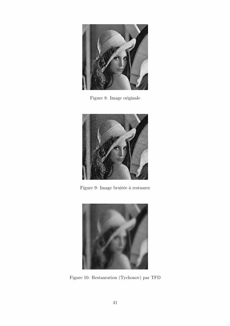
Figure 8: Image originale

Figure 9: Image bruitée à restaurer

Figure 10: Restauration (Tychonov) par TFD

41

infu∈BV (Ω)

(

J(u) +1

2λ‖f − Au‖2

2

)

(3.39)

where J(u) =∫

Ω|Du| stands for the total variation of u, and where A is a continuous and

linear operator of L2(Ω) such that A1 6= 0 (the case when A is compact is simpler).The mathematical study of (3.39) is done in [25].The proof of existence of a solution is similar to the one for the Tychonov regularization

(except that now one works in BV (Ω) instead of W 1,2(Ω). If A is assumed to be injective, thenthis solution is unique.

Sketch of the proof of existence: We denote by:

F (u) = J(u) +1

2λ‖f − Au‖2

2 (3.40)

F is convex.For the sake of simplicity, we assume that A = Id. See [9] for the detailed proof in the

general case.Let us consider un a minimizing sequence for (3.39) with A = Id. Hence there exists M > 0

such that J(un) ≤ M and ‖f − un‖22 ≤ M (M denotes a generic positive constant during the

proof). Moreover, since ‖un‖2 ≤ ‖f‖2 + ‖f − un‖2, we have ‖un‖2 ≤M . Hence un is boundedin BV (Ω). By weak-* compacity, there exists therefore u in BV (Ω) such that un → u in L1(Ω)strong and Dun Du.

By l.s.c. of the total variation, we have J(u) ≤ lim inf J(un), and by l.s.c. of the weak normwe have ‖f−u‖2 ≤ lim inf ‖f−un‖2. Hence, up to a subsequence, we have limn→+∞ inf F (un) ≥F (u).

Maximum principle (truncation argument)

Proposition 3.2. Let f be in L∞(Ω) and u be a solution of the ROF Problem with A = Id.Then a maximum principle holds for u:

infΩf ≤ u ≤ sup

Ωf (3.41)

It is based on a standard truncation argument. We remark that x 7→ (x− a)2 is decreasingif x ∈ (−∞, a) and increasing if x ∈ (a,+∞). Therefore, if M ≥ a, one always has:

(min(x,M) − a)2 ≤ (x− a)2 (3.42)

Hence, if we let M = supΩ f , we find that:∫

Ω

(min(u,M) − f)2 dx ≤∫

Ω

(u− f)2 dx (3.43)

Moreover, it is a direct consequence of the coarea formula that |D(min(u, sup f))|(Ω) ≤|Du|(Ω) which yields that the function min(u, sup f) is a solution of the ROF Problem. We getthe opposite inequality with a similar argument.

Hence we do not decrease the energy by assuming that inf f ≤ u ≤ sup f . We conclude byusing the uniqueness of the solution of the ROF problem.

42

Comparison principle We now state a comparison principle.

Proposition 3.3. Let f1 and f2 be in L∞(Ω). Let us assume that f1 ≤ f2. We denote by u1

(resp. u2) a solution of the ROF problem for f = f1 (resp. f = f2). Then we have u1 ≤ u2.

Proof We first consider the case when f1 < f2.We use here the following classical notations: u ∨ v = sup(u, v), and u ∧ v = inf(u, v).We have since ui is a minimizer with data fi:

J(u1 ∧ u2) +

∫

Ω

(f1 − u1 ∧ u2)2 ≥ J(u1) +

∫

Ω

(f1 − u1)2 (3.44)

and:

J(u1 ∨ u2) +

∫

Ω

(f2 − u1 ∨ u2)2 ≥ J(u2) +

∫

Ω

(f2 − u2)2 (3.45)

Adding these two inequalities, and using the fact that [45]:

J(u1 ∧ u2) + J(u1 ∨ u2) ≤ J(u1) + J(u2) (3.46)

we get:∫

Ω

((f1 − u1 ∧ u2)

2 − (f1 − u1)2 + (f2 − u1 ∨ u2)

2 − (f2 − u2)2)≥ 0 (3.47)

Writing Ω = u1 > u2 ∪ u1 ≤ u2, we easily deduce that:∫

u1>u2

((f1 − u2)

2 − (f1 − u1)2 + (f2 − u1)

2 − (f2 − u2)2)≥ 0 (3.48)

i.e.: ∫

u1>u22 (−f1u2 + f1u1 − f2u1 + f2u2) ≥ 0 (3.49)

i.e.: ∫

u1>u2(f2 − f1)(u2 − u1) ≥ 0 (3.50)

Since f1 < f2, we thus deduce that u1 > u2 has a zero Lebesgue measure, i.e. u1 ≤ u2 a.e.in Ω.

Now, for the general case f1 ≤ f2, we make use of the following lemma:

Lemma 3.1. ui solution of the ROF problem with data fi. Then we have:

‖u1 − u2‖2 ≤ ‖f1 − f2‖2 (3.51)

From the above lemma, the maping fi 7→ ui is continuous in L2(Ω). Hence the result

43

Proof of the lemma :We use the Euler-Lagrange equation:

fi − ui ∈ ∂J(ui) (3.52)

We make the difference of the previous equation with i = 1 and then i = 2, and multiply byu1 − u2. We get:

〈f1 − f2 − (u1 − u2), u1 − u2〉 = 〈∂J(u1) − ∂J(u2), u1 − u2〉 (3.53)

But, J being convex, it is a monotone operator, i.e. 〈∂J(u1) − ∂J(u2), u1 − u2〉 ≥ 0. Hence:

〈f1 − f2, u1 − u2〉 ≥ ‖u1 − u2‖22 (3.54)

Using Cauchy Schwartz inequality, we get:

‖u1 − u2‖22 ≤ ‖f1 − f2‖ ‖u1 − u2‖ (3.55)

and thus ‖f1 − f2, u1 − u2‖ ≤ f1 − f2‖. In particular, this implies the uniqueness of ui when fi

is fixed.

Euler-Lagrange equation: Formally, the associated Euler-Lagrange equation is:

−div( ∇u|∇u|

)

+1

λ(A∗Au− A∗f) = 0 (3.56)

with Neuman boundary conditions.Numerically, one uses a fixed point process:

∂u

∂t= div

( ∇u|∇u|

)

− 1

λ((A∗Au− A∗f) (3.57)

However, in this approach, it is needed to regularize the problem, i.e. to replace∫

Ω|Du| in

(3.39) by∫

Ω

√

|∇u|2 + ǫ2. The Euler-Lagrange equation is then:

∂u

∂t= div

(

∇u√

|∇u|2 + ǫ2

)

− 1

λ((A∗Au− A∗f) (3.58)

Moreover, when working with BV (Ω), (3.56) is not true.

Sketch of the proof:φ(x) =

√ǫ2 + x2 (3.59)

We have:|∇(u+ h)|2 = |∇u|2 + 2∇h.∇u+ o(|h|) (3.60)

Thus

√

|∇(u+ h)|2 = |∇u|(

1 +2∇h.∇u2|∇u|2

)

+ o(|h|) = |∇u| + ∇h.∇u|∇u| + o(|h|) (3.61)

44

Thus

φ (|∇(u+ h)|) = φ

(

|∇u| + ∇h.∇u|∇u| + o(|h|)

)

= φ (|∇u|) +∇h.∇u|∇u| φ′ (|∇u|) + o(|h|) (3.62)

Thus ∫

Ω

φ(u+ h) =

∫

Ω

φ(u) +

∫

Ω

−hdiv(φ′ (|∇u|)|∇u| ∇u

)

+ o(|h|) (3.63)

Since‖A(u+ h) − f‖2 = ‖Au− f‖2 + 2〈h,A∗(Au− f)〉 + o(|h|) (3.64)

We therefore have, since J(u+ h) = J(u) + 〈h,∇J(u)〉 + o(|h|):

∇J(u) = −λdiv(φ′(|∇u|)|∇u| ∇u

)

+ A∗(Au− f) (3.65)

Notice that in the case when φ(x) =√ǫ2 + x2, then φ′(x) = x√

ǫ2+x2 , and therefore

φ′(|∇u|)|∇u| =

1√

ǫ2 + |∇u|2(3.66)

For the sake of simplicity, we assume in the following that A = Id.

3.3.2 Interpretation as a projection

We are therefore interested in solving:

infu∈BV (Ω)

(

J(u) +1

2λ‖f − u‖2

2

)

(3.67)

We consider the case N = 2. J is extended to L2.Using convex analysis result, the optimality condition associated to the minimization prob-

lem (3.67) is:

u− f ∈ λ∂J(u) (3.68)

This condition is used in [24] to derive a minmization algorithm for (3.67).Since J is homogeneous of degree one (i.e. J(λu) = λJ(u) ∀u and λ > 0), it is standard (cf

[36]) that J∗ the Legendre Fenchel transform of J ,

J∗(v) = sup ((u, v)2 − J(u)) (3.69)

is the indicator function of a closed convex set K.It is easy to check that K identifies with the set (using the fact that J∗∗ = J):

K = div (g)/g ∈ (L∞(Ω))2, ‖g‖∞ ≤ 1 (3.70)

and

J∗(v) = χK(v) =

0 if v ∈ K+∞ otherwise

(3.71)

The next result is shown in [24] :

Proposition 3.4. The solution of (3.67) is given by:

u = f − PλK(f) (3.72)

where P is the orthogonal projection on λK.

45

Proof: If u is a minimizer, then

0 ∈ (u− f) /λ+ ∂J(u) (3.73)

i.e. :(f − u) /λ ∈ ∂J(u) (3.74)

Henceu ∈ ∂J∗ ((f − u) /λ) (3.75)

We set w = (f − u), and we get:

0 ∈ w − f + ∂J∗ (w/λ) (3.76)

We then deduce that w is the minimizer of:

infw

(

‖w − f‖2 +1

2λJ∗ (w/λ)

)

(3.77)

i.e. w = PλK(f), hence u = f − PλK(f).

Algorithm : [24] proposes an algorithm to compute PλK(f) which can be written in discrete:

min‖λdiv (p) − f‖2

X : p / |pi,j| ≤ 1 ∀i, j = 1, . . . , N

(3.78)

(3.78) can be solved with a fixed point process:

p0 = 0 (3.79)

and

pn+1i,j =

pni,j + τ(∇(div (pn) − f/λ))i,j

1 + τ |(∇(div (pn) − f/λ))i,j|(3.80)

And [24] gives a sufficient condition for the algorithm to converge:

Theorem 3.1. Assume that parameter τ in (3.80) is such that τ ≤ 1/8. Then λdiv(pn)converges to PλK(f) when n→ +∞.

The solution to problem (3.67) is therefore given by:

u = f − λdiv (p∞) (3.81)

where p∞ = limn→+∞ pn

46

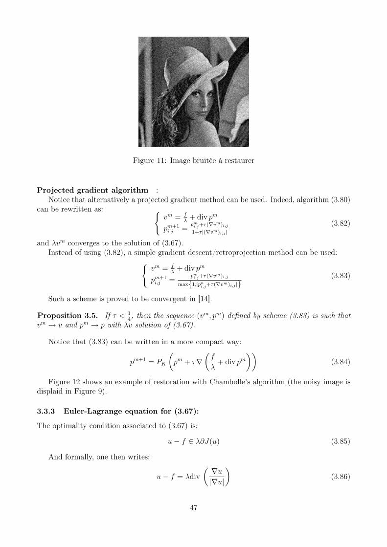
Figure 11: Image bruitée à restaurer

Projected gradient algorithm :Notice that alternatively a projected gradient method can be used. Indeed, algorithm (3.80)

can be rewritten as:

vm = fλ

+ div pm

pm+1i,j =

pmi,j+τ(∇vm)i,j

1+τ |(∇vm)i,j |(3.82)

and λvm converges to the solution of (3.67).Instead of using (3.82), a simple gradient descent/retroprojection method can be used:

vm = f

λ+ div pm

pm+1i,j =

pmi,j+τ(∇vm)i,j

max1,|pni,j+τ(∇vm)i,j |

(3.83)

Such a scheme is proved to be convergent in [14].

Proposition 3.5. If τ < 14, then the sequence (vm, pm) defined by scheme (3.83) is such that

vm → v and pm → p with λv solution of (3.67).

Notice that (3.83) can be written in a more compact way:

pm+1 = PK

(

pm + τ∇(f

λ+ div pm

))

(3.84)

Figure 12 shows an example of restoration with Chambolle’s algorithm (the noisy image isdisplaid in Figure 9).

3.3.3 Euler-Lagrange equation for (3.67):

The optimality condition associated to (3.67) is:

u− f ∈ λ∂J(u) (3.85)

And formally, one then writes:

u− f = λdiv( ∇u|∇u|

)

(3.86)

47

Figure 12: Image restaurée (ROF)

But the subdifferential ∂J(u) cannot always be written this way.The following result (see Proposition 1.10 in [6] for further details) gives more details about

the subdifferential of the total variation.

Proposition 3.6. Let (u, v) in L2(Ω) with u in BV (Ω). The following assertions are equiva-lent:

(i) v ∈ ∂J(u).

(ii) Denoting by X(Ω)2 = z ∈ L∞(Ω,R2) : div (z) ∈ L2(Ω), we have:∫

Ω

vu dx = J(u) (3.87)

and∃z ∈ X(Ω)2 , ‖z‖∞ ≤ 1 , z.N = 0 , on ∂Ωsuch that v = −div (z) in D′(Ω)

(3.88)

(iii) (3.88) holds and: ∫

Ω

(z,Du) =

∫

Ω

|Du| (3.89)

From this proposition, we see that (3.85) means:

u− f = λdiv z (3.90)

with z satisfying (3.88) and (3.89). This is a rigorous way to write u− f = λdiv(

∇u|∇u|

)

.

3.3.4 Other regularization choices

The drawback of the total variation regularization is a staircase effect. There has thereforebeen a lot of work dealing with how to remedy to this problem. In particular, people haveinvestigated other regularization choice of the kind L(u) =

∫

Ωφ(|∇u|). The functional to

minimize becomes thus:

infu

1

2‖f − Au‖2 + λ

∫

Ω

φ(‖∇u‖) dx (3.91)

48

And formally, the associated Euler-Lagrange equation is:

−λdiv(φ

′

(|∇u|)|∇u| ∇u

)

+ A∗Au− A∗f = 0 (3.92)

with Neumann boundary conditions:

φ′

(|∇u|)|∇u|

∂u

∂N= 0 on ∂Ω. (3.93)

We are now going to develop formally the divergence term. For each point x where |∇u(x)| 6=0, we can define the vectorsN(x) = ∇u(x)

|∇u(x)| and T (x), |T (x)| = 1, with T (x) ⊥ N(x), respectivelythe normal and the tangent to the level line of u.

We can then rewrite (3.92) as:

A∗Au− λ

(φ

′

(|∇u|)|∇u| uTT + φ

′′

(|∇u|)uNN

)

= A∗f (3.94)

where we denote by uTT and uNN the second derivatives of u in the T direction and Ndirection, respectively:

uTT = T ∗∇2uT =1

|∇u|2(u2

x1ux2x2 + u2

x2ux1x1 − 2ux1ux2ux1x2

)(3.95)

uNN = N∗∇2uN =1

|∇u|2(u2

x1ux1x1 + u2

x2ux2x2 + 2ux1ux2ux1x2

)(3.96)

This allows to see clearly the action of the function φ in both directions N and T .• At the location, where the variation of the intensity are weak (low gradient), we would liketo encourage smoothing, the same in all directions.

Assuming that φ is regular, this isotropic smoothing can be achieved by imposing:

φ′

(0) = 0 , lims→0+

φ′

(s)

s= lim

s→0+φ

′′

(s) = φ′′

(0) > 0 (3.97)

Therefore, at points where |∇u| is small, (3.94) becomes:

A∗Au− λφ′′

(0)(uTT + uNN︸ ︷︷ ︸

=∆u

) = A∗f (3.98)

So at these points, we want to do some Tychonov regularization.• In a neighbourhood of an edge C, the image presents a strong gradient. If we want to preservethis edge, it is preferable to diffuse along C (in the T direction) and not across it. To do so, itis sufficient in (3.94) to annihilate (for strong gradients) the coefficient of uNN , and to assumethat the coefficient of uTT does not vanish:

lims→+∞

φ′′

(s) = 0 , lims→+∞

φ′

(s)

s= β > 0 (3.99)

Unfortunately, this two conditions ar not compatible. A trade-off mus be found. For instance,

φ′′

(s) and φ′

(s)s

both converge to 0 as s→ +∞, but at different rates:

lims→+∞

φ′′

(s) = lims→+∞

φ′

(s)

s= 0 and lim

s→+∞

φ′′

(s)φ′(s)s

= 0 (3.100)

49

For instance, one may choose the hypersurface minimal function:

φ(s) =√

1 + s2 (3.101)

Of course, all these remarks are qualitative. Other conditions will arise so that the problem ismathematically well-posed.

To show the existence and uniqueness of a solution using the direct method of the calculusof variations, some minimal hypotheses are needed on φ:

(i) φ is strictly convex, nondecreasing function from R+ to R

+, with φ(0) = 0 (without a lossof generality).

(ii) lims→+∞ φ(s) = +∞.

Conditions (ii) must not be too strong, because it must not penalize strong gradients, i.e.the formation of edges (see what happens if φ(s) = s2). Hence we assume that φ grows at mostlinearly: there exist two constants c > 0 and b ≥ 0 such that:

cs− b ≤ φ(s) ≤ cs+ b for all s ≥ 0 (3.102)

With all these assumptions, it then possible to show that problem (3.91) admits a uniquesolution in BV (Ω) (see [9]).

Non convex φ function: It has been shown numerically that the choice of non convex φfunctions can lead to very interisting results [9]. Nevertheless, in the continuous case, the directmethod of calculus of variation fails to prove the existence of a solution for such regularizationchoices. This remains an open question. In particular, the following functions have been shownto give good restoration results:

φ(s) =s2

1 + s2(3.103)

and:

φ(s) = log(1 + s2) (3.104)

3.3.5 Half quadratic minimmization

J(u) = λ

∫

Ω

φ(|∇u|) dx+1

2‖f − Au‖2 (3.105)

with φ edge preserving function [9]. φ C1 and convex. Typically:

φ(x) =√ǫ2 + x2 (3.106)

We have already seen before that:

∇J(u) = −λdiv(φ′(|∇u|)|∇u| ∇u

)

+ A∗(Au− f) (3.107)

Notice that in the case when φ(x) =√ǫ2 + x2, then φ′(x) = x√

ǫ2+x2 , and therefore φ′(|∇u|)|∇u| =

1√ǫ2+|∇u|2

.

50

Fixed step gradient descent The easiest method is a fixed step gradient descent [65].

uk+1 = uk − δt∇J(uk) (3.108)

Nevertheless, it is quite slow: indeed, for the algorithm to converge , δt needs to be verysmall. In particular, if φ(x) =

√ǫ2 + x2, then a typical choice for δt is δt = ǫ/10.

Quasi-Newton method To improve the speed of the above algorithm, it has been tried touse Newton method:

uk+1 = uk − (∇2J(uk))−1∇J(uk) (3.109)

But in practice this is not possible.In the case when φ(x) =

√ǫ2 + x2, we have

∇J(u) = −λdiv

(

1√

ǫ2 + |∇u|2∇u)

+ A∗(Au− f) (3.110)

We are interested in solving ∇J(u) = 0. Since we do not know how to invert ∇J , we want touse a fixed point process. We linearize the equation (quasi-Newton method):

0 = −λdiv

(

1√

ǫ2 + |∇uk|2∇uk+1

)

+ A∗(Auk+1 − f) (3.111)

It is natural to look at a semi-explicit scheme, explicit in the non linear part and implicit inthe linear part (general idea of Weiszfeld method [73]), i.e.:

uk+1 =

(

A∗A.− λdiv

(

1√

ǫ2 + |∇uk|2∇.))−1

A∗f (3.112)

It can be shown that such a scheme converges to the solution [1, 70, 34, 27, 3]. Moreover, itis much faster than a gradient descent (it is possible to show theoretically a linear convergence,but in practice a quadratic convergence is observed).

For a general φ C1 function the scheme is:

0 = −λdiv(φ′(|∇uk|φ(|∇uk|)

∇uk+1

)

+ A∗(Auk+1 − f) (3.113)

uk+1 =

(

A∗A.− λdiv(φ′(|∇uk|φ(|∇uk|)

∇.))−1

A∗f (3.114)

This is in fact a special case of a more general method: the half quadratic minimizationapproach [9].

Half quadratic minimization approach It is based on the following result.

Proposition 3.7. Let φ : R+ → R+ a non decreasing function such that φ(√t) concave. Let

us define:

L = limt→+∞

φ′(t)

2tand M = lim

t→0+

φ′(t)

2t(3.115)

51

Then there exists a convex and decreasing function ψ : (L,M ] → [β1, β2] such that:

φ(s) = infL≤b≤M

(bs2 + ψ(b)) (3.116)

where β1 = lims→0+ φ(s) and β2 = lims→+∞(φ(s) − sφ′(s)/2).Moreover, the value b for which the minimum is reached is given by:

b =φ′(s)

2s(3.117)

The additional variable b is usually called the dual variable.

Proof: Let θ(s) = −φ(√s). θ is a convex function. Thus

θ(s) = θ∗∗(s) = sups∗

(ss∗ − θ∗(s∗)) (3.118)

where θ∗(s∗) is the polar funtion of θ(s) defined by: θ∗(s∗) = sups(ss∗ − θ(s)). Therefore:

φ(√s) = inf

s∗(−ss∗ + θ∗(s∗)) (3.119)

Let b = −s∗ and s =√s. Then φ can be written:

φ(s) = infs∗

(bs2 + θ∗(−b)) (3.120)

which gives the first part of the theorem with

ψ(b) = θ∗(−b) (3.121)

The rest of the proof is standard.

Remark: Let us emphasize that in the above proposition, φ can be non convex.For instance, when φ(s) = s2

1+s2 , then ψ(b) = (√b− 1)2, L = 0, and M = 1.

Application:

J(u) = λ

∫

Ω

φ(|∇u|) dx+1

2‖f − Au‖2 (3.122)

Assume φ satisfies the hypotheses of the previous proposition. Then we have:

J(u) = λ

∫

Ω

infL≤b≤M

(bs2 + ψ(b))|∇u| dx+1

2‖f − Au‖2 (3.123)

Supposing we can invert∫

Ωand the infimum (this can be justified):

infuJ(u) = inf

uinfb

(

λ

∫

Ω

(b|∇u|2 + ψ(b)) dx+1

2‖f − Au‖2

)

= infb

infu

(

λ

∫

Ω

(b|∇u|2 + ψ(b)) dx+1

2‖f − Au‖2

)

52

Let us define

F (u, b) = λ

∫

Ω

(b|∇u|2 + ψ(b)) dx+1

2‖f − Au‖2 (3.124)

This functional is convex in u, and for each u fixed it is convex in b (but the functional isnot convex with respect to the pair (u, b)).

It can be shown that alternating minmizations with respect to u and v, then uk converges tothe minimizer u of the original functional [9, 28, 25]. Moreover, this is a much faster algorithmthan the fixed step gradient algorithm.

The sequence bk can be seen as an indicator of contours. If φ satisfies the edge-preservinghypotheses lims→+∞ φ′(s)/(2s) = 0 and lims→+0+ φ′(s)/(2s) = 1, then the following conditionsare satisfied:

• If bk(x) = 0, then x belongs to a contour.

• If bk(x) = 1, then x belongs to a homogeneous region.

At each iteration, we define:

uk+1 = argminu

F (u, bk) (3.125)

andbk+1 = argmin

bF (uk+1, b) (3.126)

We have

bk+1 =φ′(|∇uk+1|)2|∇uk+1|

(3.127)

and uk+1 is the solution of:

0 = −λdiv (2bk∇u) + A∗(Au− f) (3.128)

which can be solved with a conjugate gradient algorithm.Notice that in the case when φ(x) =

√ǫ2 + x2, this is in fact exactly the same scheme as

above.

3.4 Wavelets

3.4.1 Besov spaces

We denote by ψj,k a wavelet basis. A function f in L2(R2) can be written:

f =∑

j,k

cj,kψj,k (3.129)

where the cj,k are the wavelet coefficients of f , and we have: ‖f‖L2(R2) =∑

j,k c2j,k.

Spaces weel-suited to wavelets are Besov spaces Bsp,q (for 0 < s < ∞, 0 < p ≤ ∞ and

0 < q ≤ ∞) [57, 55, 30, 25]. Bsp,q correponds roughly to functions with s derivatives in Lp(R2),

the third parameter q being a way to adjust the regularity with precision.

53

Remark: if p = q = 2, then Bs2,2 is the Sobolev space W s,2, and when s < 1, 1 ≤ p ≤ ∞, and

q = ∞, then Bsp,∞ is the Lipschitz space Lip(s, Lp(R2)).

We can give an intrinsic definition to Besov spaces Bsp,q and of their norm ‖.‖Bs

p,qfrom the

regularity modulus of f [30, 25]. If we assume that the chosen wavelet ψ has at least s + 1vanishing moments and is of regularity at least Cs+1, then if f ∈ Bs

p,q, the norm ‖f‖Bsp,q

isequivalent to:

∑

k

(∑

j

2skp2k(p−2)|cj,k|p) p

q

1q

(3.130)

(the constants depend on the chosen wavelet).In what follows, we will always use the equivalent norm (3.130) for ‖f‖Bs

p,q.

Here, we are interested in homogeneous version of Besov spaces:

˙Bsp,q = Bs

p,q/u ∈ Bs

p,q / ∇u = 0

(3.131)

Definition 3.1. B11,1 is the usual homogeneous Besov space (cf [57]). Let ψj,k an orthonormal

wavelet basis composed of regular wavelets with compact supports. B11,1 is a subspace of L2(R2)

and a function f belongs to B11,1 if and only of:

∑

j∈Z

∑

k∈Z2

|cj,k|2j/2 < +∞ (3.132)

Definition 3.2. The dual space of B11,1 is the Banach space B∞

−1,∞. It is characterized by thefact that the wavelet function of a generalized function in B∞

−1,∞ are in l∞(Z × Z2).

Remark: We have the following inclusions:

B11,1 ⊂ ˙BV (R2) ⊂ L2(R2) ⊂ B∞

−1,∞ (3.133)

where ˙BV stands for the homogeneous version of BV : ˙BV = BV/ u ∈ BV / ∇u = 0.

3.4.2 Wavelet shrinkage

A interesting application of wavelets is image denoising. If an original image u has beendegraded by some additive white gaussian noise, an efficient restoration method consists inthresholding the wavelet coefficients of the degraded image f .

We define the soft-thresholding operator as:

θτ (t) =

t− τ if t ≥ τ0 if t ≤ τt+ τ si t ≤ −τ

(3.134)

In an orthonormal wavelet basis, the wavelet coefficients of f denoted by cj,k(f) are randomgaussian variables with zero mean with standard deviation σ (σ being the standard deviationof the white gaussian noise).

The wavelet soft-thresholding of f with parameter τ , denoted by WST (f, τ) (Wavelet SoftThresholding), is the function whose wavelet coefficients are θτ (cj,k(f)). The theoretical valueproposed by Donoho is τ = σ

√

2 log(N2), where N2 stands for the size of the image (in practice,this threshold value is much too large). For further details, we refer the reader to [35, 53, 57, 55].

54

Figure 13: Restoration by non invariant wavelet shrinkage (Haar)

3.4.3 Variational interpretation

Let us consider the functionalinfu‖f − u‖2 + 2τ‖u‖B1

1,1(3.135)

The solution to (3.135) is given by:

u = WST (f, τ) (3.136)

Sketch of the proof: (see [25] for the detailed proof)Denote by cj,k (resp. dj,k ) the wavelet coefficients of f (resp. u). We thus have to minimize:

∑

j,k

(|cj,k − dj,k|2 + 2τ |dj,k|

)(3.137)

There is no coupling term in the equations, and we therefore just have to minimize thegeneric function

E(s) = |s− t|2 + 2τ |s| = |s|2 + 2|s|(τ − |t|) + t2 (3.138)

We minimize f(x) = x2 + 2x(τ − |t|) + t2 with the constraint x ≥ 0. We have f ′(x) =2x+ 2(τ − |t|).

Figure 13 and 14 show examples of restoration.

Remark: In 1D, total variation minimization is equivalent to iterative wavelet shrinkage(using the Harr wavelet with one level of decomposition) [67].

55

Figure 14: Restoration by invariant wavelet shrinkage (Haar)

4. Advanced topics: Image decomposition

We encourage the reader to look at [57] for a nice historical introduction to the topics.

4.1 Introduction

Image restoration is an important and challenging inverse problem in image analysis. Theproblem consists in reconstructing an image u from a degraded data f . The most commonmodel linking u to f is the following one: f = Ru + v , where R is a linear operator typicallymodeling blur and v is the noise. Energy minimization has demonstrated to be a powerfulapproach to tackle this kind of problem (see [9] and references therein for instance). Here weexamine a pure denoising situation, i.e. R is the identity operator. The underlying energy isgenerally composed of two terms: a fidelity term to the data and a regularizing-cost function.One of the most effective method is the total variation minimization as proposed in [65]. Thismodel relies on the assumption that BV (Ω), the space of functions with bounded variation, isa good space to study images (even if it is known that such an assumption is too restrictive[4]). In [65], the authors decompose an image f into a component u belonging to BV (Ω) and acomponent v in L2(Ω). In this model v is supposed to be the noise. In such an approach, theyminimize:

inf(u,v)∈BV (Ω)×L2(Ω)/f=u+v

(∫

|Du| + 1

2λ‖v‖2

L2(Ω)

)

(4.1)

where∫|Du| stands for the total variation of u. In practice, they compute a numerical solution

of the Euler-Lagrange equation associated to (4.1). The mathematical study of (4.1) has beendone in [25].

In [57], Y. Meyer shows some limitations of the model proposed in [65]. In particular, if f isthe characteristic function of a bounded domain with a C∞-boundary, then f is not preservedby the Rudin-Osher-Fatemi model (contrary to what should be expected).

56

Meyer model In [57], Y. Meyer suggests a new decomposition. He proposes the followingmodel:

inf(u,v)∈BV (R2)×G(R2)/f=u+v

(∫

|Du| + α‖v‖G(R2)

)

(4.2)

where the Banach space G(R2) contains signals with large oscillations, and thus in particulartextures and noise. We give here the definition of G(R2).

Definition 4.1. G(R2) is the Banach space composed of distributions f which can be written

f = ∂1g1 + ∂2g2 = div (g) (4.3)

with g1 and g2 in L∞(R2). The space G(R2) is endowed with the following norm:

‖v‖G(R2) = inf

‖g‖L∞(R2) = ess supx∈R2

|g(x)| /v = div (g), g = (g1, g2),

g1 ∈ L∞(R2), g2 ∈ L∞(R2), |g(x)| =√

(|g1|2 + |g2|2)(x)

(4.4)

BV (R2) has no simple dual space (see [5]). However, as shown by Y. Meyer [57], G(R2)is the dual space of the closure in BV (R2) of the Schwartz class. So it is very related to thedual space of BV (R2). This is a motivation to decompose a function f on BV (R2) + G(R2).This is also why the divergence operator naturally appears in the definition of G(R2), since thegradient and the divergence operators are dual operators.

A function belonging to G may have large oscillations and nevertheless have a small norm.Thus the norm on G is well-adapted to capture the oscillations of a function in an energyminimization method.

4.2 A space for modeling oscillating patterns in bounded domains

4.2.1 Definition and properties

In all the sequel, we denote by Ω a bounded connected open set of R2 with a Lipschitz boundary.

We adapt Definition 4.1 concerning the space G to the case of Ω. We are going to consider asubspace of the Banach space W−1,∞(Ω) =

(W 1,1

0 (Ω))′

(the dual space of W 1,10 (Ω)).

Definition 4.2. G(Ω) is the subspace of W−1,∞(Ω) defined by:

G(Ω) =v ∈ L2(Ω) / v = div ξ , ξ ∈ L∞(Ω,R2) , ξ.N = 0 on ∂Ω

(4.5)

On G(Ω), the following norm is defined:

‖v‖G(Ω) = inf‖ξ‖L∞(Ω,R2) /v = div ξ , ξ.N = 0 on ∂Ω

(4.6)

Remark: In Definition 4.2, since div ξ ∈ L2(Ω) and ξ ∈ L∞(Ω,R2), we can define ξ.N on ∂Ω(in this case, ξ.N ∈ H−1/2(∂Ω), see [68, 52] for further details).

57

The next lemma was stated in [57]. Using approximations with C∞c (Ω) functions [5], the

proof is straightforward:

Lemma 4.1. Let u ∈ BV (Ω) and v ∈ G(Ω). Then:∫

Ωuv ≤ J(u)‖v‖G(Ω) (where J(u) is

defined by (2.70)).

We have the following simple characterization of G(Ω):

Proposition 4.1.

G(Ω) =

v ∈ L2(Ω) /

∫

Ω

v = 0

(4.7)

Proof: Let us denote by H(Ω) the right-hand side of (4.7). We split the proof into two steps.Step 1: Let v be in G(Ω). Then from(4.5) it is immediate that

∫

Ωv = 0, i.e. v ∈ H(Ω).

Step 2: Let v be in H(Ω). Then from [21] (Theorem 3’) (see also [22]), there exists ξ ∈C0(Ω,R2) ∩ W 1,2(Ω,R2) such that v = div ξ and ξ = 0 on ∂Ω. In particular, we have ξ ∈L∞(Ω,R2) and ξ.N = 0 on ∂Ω. Thus v ∈ G(Ω).

Remark: Let us stress here how powerful the result in [22, 21] is. It deals with the limit casev in Lq(Ω), q = 2, when the dimension of the space is N = 2. The classical method for tacklingthe equation div ξ = v with ξ.N = 0 on ∂Ω consists in solving the problem ∆u = v with ∂u

∂N= 0

on ∂Ω, and in setting ξ = ∇u. If v is in Lq(Ω) with q > 2 this problem admits a unique solution(up to a constant) in W 2,q(Ω). Moreover, thanks to standard Sobolev embeddings (see [37, 40]),ξ = ∇u belongs to L∞(Ω,R2). If q = 2, the result is not true and the classical approach doesnot work. So the result by Bourgain and Brezis is very sharp.

We next introduce a family of convex subsets of G(Ω). These convex sets will be useful forapproximating Meyer problem.

Definition 4.3. Let Gµ(Ω) the family of subsets defined by (µ > 0):

Gµ(Ω) =v ∈ G(Ω) / ‖v‖G(Ω) ≤ µ

(4.8)

Lemma 4.2. Gµ(Ω) is closed for the L2(Ω)-strong topology.

Proof of Lemma 4.2 Let (vn) be a sequence in Gµ(Ω) such that there exists v ∈ L2(Ω)with vn → v in L2(Ω)-strong. We have vn = div ξn, with ξn such that ‖ξn‖L∞(Ω,R2) ≤ µ andξn.N = 0 on ∂Ω. As ‖ξn‖L∞(Ω,R2) ≤ µ, there exists ξ ∈ L∞(Ω,R2) such that, up to an extraction:ξn ξ in L∞(Ω,R2) weak * , and ‖ξ‖L∞(Ω,R2) ≤ µ.

Moreover if φ ∈ D(Ω):∫

Ωvnφ dx =

∫

Ωdiv ξnφ dx = −

∫

Ωξn∇φ dx. Thus as n → +∞, we

get: ∫

Ω

vφ dx = −∫

Ω

ξ∇φ dx =

∫

Ω

div ξ φ dx−∫

∂Ω

ξ.Nφ (4.9)

By choosing first a test function in C∞c (Ω), we deduce from (4.9) that v = div ξ in D′(Ω), and

since v ∈ L2(Ω), the equality holds in L2(Ω). Then for a general φ ∈ D(Ω), it comes ξ.N = 0on ∂Ω (in H−1/2(∂Ω)).

58

The next result is a straightforward consequence of Lemma 4.2.

Corollary 4.1. The indicator function of Gµ(Ω) is lsc (lower-semicontinuous) for the L2(Ω)-strong topology (and for the L2(Ω)-weak topology since Gµ is convex).

Remarks:

1. Let us denote by K(Ω) the closure in L2(Ω) of the set:div ξ , ξ ∈ C∞

c (Ω,R2) , ‖ξ‖L∞(Ω,R2) ≤ 1

(4.10)

Using Lemma 4.2 and some results in [68], one can prove that K(Ω) = G1(Ω).

Moreover, one can also show in the same way that G(Ω) is the closure in L2(Ω) of theset:

div ξ , ξ ∈ C∞

c (Ω,R2)

(4.11)

2. From the proof of Lemma 4.2, one easily deduces that ‖.‖G is lower semi continuous (lsc).

We also have the following result:

Lemma 4.3. If v ∈ G(Ω), then there exists ξ ∈ L∞(Ω,R2) with v = div ξ and ξ.N = 0 on∂Ω, and such that ‖v‖G = ‖ξ‖L∞(Ω,R2).

Proof: Let v ∈ G(Ω). Let us consider a sequence ξn ∈ L∞(Ω,R2) with v = div ξn andξn.N = 0 on ∂Ω, and such that ‖ξn‖L∞(Ω) → ‖v‖G. There exists ξ ∈ L∞(Ω,R2) such that, upto an extraction, ξn ξ in L∞(Ω,R2) weak *. Then, as in the proof of Lemma 4.2, we canshow that ξ.N = 0 on ∂Ω and that v = div ξ.

Main property: The following lemma is due to Y. Meyer [57]. But it was stated in the caseof Ω = R

2, and the proof relied upon harmonic analysis tools. Thanks to our definition ofG(Ω), we formulate it in the case when Ω is bounded. Our proof relies upon functional analysisarguments.

Lemma 4.4. Let Ω be a Lipschitz bounded open set, and let fn , n ≥ 1 be a sequence offunctions in Lq(Ω)

⋂G(Ω) with the following two properties:

1. There exists q > 2 and C > 0 such that ‖fn‖Lq(Ω) ≤ C.

2. The sequence fn converges to 0 in the distributional sense (i.e. in D′(Ω)).

Then ‖fn‖G converges to 0 when n goes to infinity.

This result explains why the norm in G(Ω) is a good norm to tackle signals with strongoscillations. It will be easier with this norm to capture such signals in a minimization processthan with a classical L2-norm.

59

Remark: Hypotheses 1. and 2. are equivalent to the simpler one: there exists q > 2 suchthat fn 0 in Lq(Ω)-weak.

Proof of Lemma 4.4: Let us consider a sequence fn ∈ Lq(Ω)⋂G(Ω) satisfying assumption

1. and let us define the Neumann problem:

∆un = fn in Ω∂un

∂N= 0 on ∂Ω

(4.12)

We recall that as fn ∈ G(Ω), we also have∫

Ωfn dx = 0. We know (see [46, 59, 33]) that problem

(4.12) admits a solution un ∈ W 2,q(Ω). From [59, 58], we also know that there exists a constantB > 0 such that: ‖un‖W 2,q(Ω) ≤ B‖fn‖Lq(Ω). And as we assume that ‖fn‖Lq(Ω) ≤ C, we get:

‖un‖W 2,q(Ω) ≤ BC (4.13)

Since q > 2 and Ω bounded, we know (see [2]) that there exists θ ∈ (0, 1) such thatW 2,q(Ω) is compactly embedded in C1,θ(Ω). We denote by gn = ∇un. We have ‖gn‖W 1,q(Ω) ≤‖un‖W 2,q(Ω) ≤ BC. And it is also standard that W 1,q(Ω)2 is compactly embedded in C0,θ(Ω)2.

Hence, up to an extraction, we get that there exists u and g ∈ C0,θ such that un → u andgn → g (for the C0,θ topology). It is then standard to pass to the limit in (4.12) to deducethat gn → 0 uniformly (we recall that gn = ∇un). The previous reasonning being true for anysubsequence extracted from un, we conclude that the whole sequence ∇un is such that ∇un → 0as n → +∞ in L∞(Ω,R2)-strong, i.e. gn = ∇un → 0 in L∞(Ω,R2)-strong. Since fn = div gn,we easily deduce that ‖fn‖G → 0.

4.2.2 Study of Meyer problem

We are now in position to carry out the mathematical study of Meyer problem [57].Let f ∈ Lq(Ω) (with q ≥ 2). We recall that the considered problem is:

inf(u,v)∈BV (Ω)×G(Ω)/f=u+v

(J(u) + α‖v‖G(Ω)

)(4.14)

where J(u) is the total variation |Du| defined by (2.70).

Remark: Since f is an image, we know that f ∈ L∞(Ω). Thus it is not restrictive to supposeq ≥ 2.

Before considering problem (4.14), we first need to show that we can always decompose afunction f ∈ Lq(Ω) into two components (u, v) ∈ BV (Ω) ×G(Ω).

Lemma 4.5. Let f ∈ Lq(Ω) (with q ≥ 2). Then there exists u ∈ BV (Ω) and v ∈ G(Ω) suchthat f = u+ v.

Proof: Let us choose u = 1|Ω|∫

Ωf and v = f−u = f− 1

|Ω|∫

Ωf . We therefore have u ∈ BV (Ω)

(since Ω is bounded), and v ∈ L2(Ω). Moreover, since∫

Ωv = 0 we deduce from Proposition 4.7

that v ∈ G(Ω).

60

We now show that problem (4.14) admits at least one solution.

Proposition 4.2. Let f ∈ Lq(Ω) (with q ≥ 2). Then there exists u ∈ BV (Ω) and v ∈ G(Ω)such that f = u+ v, and:

J(u) + α‖v‖G = inf(u,v)∈BV (Ω)×G(Ω)/f=u+v

(J(u) + α‖v‖G) (4.15)

Proof: Let us first remark that the functional to minimize in (4.14) is convex with respect toits two variables. Moreover, the infimum in (4.14) is finite (thanks to Lemma 4.5).

Now, let (un, vn) be a minimizing sequence for (4.14) We thus have for some constant C

J(un) ≤ C and ‖vn‖G ≤ C (4.16)

From Poincaré inequality (see [5]), there exists a constantB > 0 such that: ‖un−∫

Ωun‖L2(Ω) ≤

BJ(un). Thus from (4.16), we get ‖un −∫

Ωun‖L2(Ω) ≤ BC. But as un + vn = f , we have:

∫

Ω

un +

∫

Ω

vn

︸ ︷︷ ︸

=0 since vn ∈ G(Ω)

=

∫

Ω

f (4.17)

Hence un is bounded in L2(Ω). From (4.16), we deduce that un is bounded in BV (Ω). Thusthere exists u ∈ BV (Ω) such that un u in BV (Ω) weak *. And as un+vn = f , we deduce thatvn is also bounded in L2(Ω). Therefore, there exists v ∈ L2(Ω) such that, up to an extraction,vn v in L2(Ω) weak.

To conclude, there remains to prove that (u, v) is a minimizer of J(u) +α‖v‖G(Ω). And thislast point comes from the fact that J is lower semi-continuous (lsc) with respect to the BVweak * topology [5], and from the fact that ‖.‖G is lsc with respect to the L2-weak topology.

Remark: It has been shown that Meyer problem can admit several solutions [47].

4.3 Decomposition models and algorithms

The problem of image decomposition has been a very active field of research during the last pastfive years. [57], was the inspiration source of many works [69, 63, 16, 8, 66, 17, 19, 26, 32, 76].

This is a hot topic in image processing. We refer the reader to the UCLA CAM reports webpage where he can find numerous papers dealing with this subject.

4.3.1 Which space to use?

We have the following result (stated in [57]):

B11,1 ⊂ ˙BV ⊂ L2 ⊂ G ⊂ E = B∞

−1,∞ (4.18)

where ˙BV is the homogeneous version of BV : ˙BV = BV/ u ∈ BV / ∇u = 0.In Figure 15, the three images have the same L2 norm. Table 1 presents the values of

different norms. It clearly illustrates the superiority of the G norm over the L2 norm to captureoscillating patterns in minimization processes (the G norm is much smaller for the texture

61

Table 1: A striking example (see Figure 15)

Images TV L2 ‖.‖−1,2 G E (Daub10)

textured image 1 000 000 9 500 33 000 360 749geometric image 64 600 9 500 300 000 2000 355

Gaussian noise (σ = 85) 2 100 000 9 500 9 100 120 287

textured image geometric image Gaussian noise (σ = 85)

Figure 15: A striking example

image and the noise image than the geometric image), as claimed in [57]. It also illustrates whythe use of the E norm is well adapted to separate the noise (the noisy image has the smallestE norm). These observations were the starting point of the decomposition algorithm by Aujoland Chambolle in [17] which split an image into three components: geometry, texture, andnoise.

More generally, the choice of the functional space used in the modelling depend on theobjective. The main advantage for using Besov spaces is their link with wavelet coefficients:this enables fast multi-scale algorithms. The main advantage of Sobolev spaces is their linkwith PDEs: an energy involving Sobolev norms can easily be minimized by solving it associatedEuler-Lagrange equation. The main advantage of BV is that contrary to Sobolev or Besovspaces, it contains charcateristic functions: in particular, any piecewise regular function is inBV , which is the reason why BV is a good candidate to model the geometrical part of animage.

Wavelet based alternative to BV have been proposed in the literature. The most popularchoice is B1

1,1. The main advantage of choosing B11,1 is that it often leads to wavelet shrinkage

algorithm, and therefore very fast algorithms. And visually it gives very similar results to BV[67, 16].

Another wavelet based alternative to BV has recently been proposed in [47] with B11,∞.

This space is closer to BV then B11,1. But the drawback is that it does not lead to wavelet

shrinkage algorithm, and therefore no fast algorithms have been proposed up to now.

4.3.2 Parameter tuning

When intereted in the general decomposition problem:

EStructure(u) + λETexture(v), f = u+ v, (4.19)

We denote by (uλ, vλ) its solution (which is assumed to exist and to be unique). The problem

62

is then to find the right regularization parameter λ. The goal is to find the right balance betweenthe energy terms which produces a meaningful structure-texture decomposition.

For the denoising problem, one often assumes that the variance of the noise σ2 is knowna-priori or can be well estimated from the image. As the v part in the denoising case shouldcontain mostly noise, a natural condition is to select λ such that the variance of v is equal tothat of the noise, that is var(v) = σ2. Such a method was used in [65] in the constrained ROFmodel, and this principle dates back to Morozov [60] in regularization theory. Here we do notknow of a good way to estimate the texture variance, also there is no performance criterion likethe SNR, which can be optimized. Therefore we should resort to a different approach.

The approach follows the work of Mrazek-Navara [61], used for finding the stopping time fordenoising with nonlinear diffusions. The method relies on a correlation criterion and assumesno knowledge of noise variance. As shown in [42], its performance is inferior to the SNR-basedmethod of [42] and to an analogue of the variance condition for diffusions. For decomposition,however, the approach of [61], adopted for the variational framework, may be a good basic wayfor the selection of λ.

Let us define first the (empirical) notions of mean, variance and covariance in the discretesetting of N ×N pixels image. The mean is

q.=

1

N2

∑

1≤i,j≤N

qi,j,

the variance isV (q)

.=

1

N2

∑

1≤i,j≤N

(qi,j − q)2,

and the covariance is

covariance(q, r) .=

1

N2

∑

1≤i,j≤N

(qi,j − q)(ri,j − r).

We would like to have a measure that defines orthogonality between two signals and is notbiased by the magnitude (or variance) of the signals. A standard measure in statistics is thecorrelation, which is the covariance normalized by the standard deviations of each signal:

correlation(q, r).=

covariance(q, r)√

V (q)V (r).

By the Cauchy-Schwarz inequality it is not hard to see that covariance(q, r) ≤√

V (q)V (r)and therefore |correlation(q, r)| ≤ 1. The upper bound 1 (completely correlated) is reachedfor signals which are the same, up to an additive constant and up to a positive multiplicativeconstant. The lower bound −1 (completely anti-correlated) is reached for similar signals butwith a negative multiplicative constant relation. When the correlation is 0 we refer to thetwo signals as not correlated. This is a necessary condition (but not a sufficient one) forstatistical independence. It often implies that the signals can be viewed as produced by different“generators" or models.

To guide the parameter selection of a decomposition we use the following assumption:

Assumption: The texture and the structure components of an image are not correlated.This assumption can be relaxed by stating that the correlation of the components is very

low. Let us define the pair (uλ, vλ) as the one minimizing (4.19) for a specific λ. As proved

63

in [57] for the TV − L2 model (and in [41] for any convex structure energy term with L2), wehave covariance(uλ, vλ) ≥ 0 for any non-negative λ and therefore

0 ≤ correlation(uλ, vλ) ≤ 1, ∀λ ≥ 0. (4.20)

This means that one should not worry about negative correlation values. Note that positivecorrelation is guaranteed in the TV − L2 case. In the TV − L1 case we may have negativecorrelations, and should therefore be more careful.

Following the above assumption and the fact that the correlation is non-negative, to findthe right parameter λ, we are led to consider the following problem:

λ∗ = argminλ (correlation(uλ, vλ)) . (4.21)

In practice, one generates a scale-space using the parameter λ (in our formulation, smaller λmeans more smoothing of u) and selects the parameter λ∗ as the first local minimum of thecorrelation function between the structural part u and the oscillating part v.

This selection method can be very effective in simple cases with very clear distinctionbetween texture and structure. In these cases correlation(u, v) behaves smoothly, reaches aminimum approximately at the point where the texture is completely smoothed out from u,and then increases, as more of the structure gets into the v part. The graphs of correlation(u, v)in the TV − L2 case behave quite as expected, and the selected parameter lead to a gooddecomposition.

For more complicated images, there are textures and structures of different scales and thedistinction between them is not obvious. In terms of correlation, there is no more a singleminimum and the function may oscillate.

As a first approximation of a decomposition with a single scalar parameter, we suggest tochoose λ after the first local minimum of the correlation is reached. In some cases, a sharpchange in the correlation is also a good indicator: after the correlation sharply drops or beforea sharp rise.

4.3.3 TV −G algorithms

infu

∫

Ω

|Du| + λ‖f − u|G (4.22)

Vese-Osher model L. Vese and S. Osher were the first authors to numerically tackle Meyerprogram [69]. They actually solve the problem:

inf(u,v)∈BV (Ω)×G(Ω)

(∫

|Du| + λ‖f − u− v‖22 + µ‖v‖G(Ω)

)

(4.23)

where Ω is a bounded open set. To compute their solution, they replace the term ‖v‖G(Ω) by‖√

g21 + g2

2‖p (where v = div (g1, g2)). Then they formally derive the Euler-Lagrange equationsfrom (4.23). For numerical reasons, the authors use the value p = 1 (they claim they madeexperiments for p = 1 . . . 10, and that they did not see any visual difference). They report goodnumerical results. See also [63] for another related model concerning the case λ = +∞ andp = 2.

64

A2BC model Inspired from the work by A. Chambolle [24], the authors of [16, 15] proposea relevant approach to solve Meyer problem. They consider the following functional defined onL2(Ω) × L2(Ω):

Fλ,µ(u, v) =

∫

Ω|Du| + 1

2λ‖f − u− v‖2

L2(Ω) if (u, v) ∈ BV (Ω) ×Gµ(Ω)

+∞ otherwise(4.24)

where Gµ(Ω) =v ∈ G(Ω) / ‖v‖G(Ω) ≤ µ

. And the problem to solve is:

infL2(Ω)×L2(Ω)

Fλ,µ(u, v) (4.25)

The authors of [16] present their model in a discrete framework. They carry out a completemathematical analysis of their discrete model, showing how it approximately solves Meyer prob-lem.

Second order cone programming approach In [76], the authors use second order coneprogramming to compute the solution. In [49], a saddle point formulation is used. And in [72],general convex minimization algorithms are applied successfully to compute the solution.

4.3.4 TV − L1

The use of the L1 norm in image processing has first been proposed in [62] to remove outliers(salt and pepper noise case). The algorithm used in [62] was a relaxation algorithm (andtherefore quite slow). The model in this case can be written:

infu

∫

Ω

|Du| + λ‖f − u‖L1 (4.26)

It was later studied from a mathematical point of view in [26], the numerical implementationbeing done with PDEs, but still quite slow (because of the singularity of the L1 norm. Analternative approach was proposed in [12] with the functional:

infu,v

∫

Ω

|Du| + µ‖f − u− v‖2L2 + λ‖v‖L1 (4.27)

By alternating minimization with respect to u and v, the solution is easily computed. Noticethat minimization with respect to u amounts to classical total variation minimization, whileminimization with respect to v is directly solved by thresholding v. Figure 16 shows an exampleof decomposition with this approach.

A fast algorithm was eventually proposed in [31]. Moreover, the authors of [31] show that(4.26) enjoys the nice property of being a contrast invariant filter.

A direct approach based on second order cone programming was proposed in [74]. Moreover,the same authors made a comparison in [75] between the classical TV − L2 model (4.1), theTV − G model (4.22), and TV − L1 (4.26). Their conclusion is that TV − L1 seems to bringbetter decomposition result (at least with synthetic images, where the user knows exactly whatis the structure and what are the textures), although the differences are not that large with theTV − G model. In any case, the classical TV − L2 is worse, mainly due to its eroding effect(which implies that some of the structure always appears in the texture component).

65

Original image

u v

Figure 16: Approximation of the TV-L1 decomposition of non-geometric texture.

Nevertheless, one should notice that the decomposition algorithm choice should be ledby the developped application: indeed, depending whether is it a first step towards imageinpainting, image compression, . . . , the required properties of the algorithm can be slightydifferent. Moreover, all the proposed approaches assume that the user knows how to tune theparameter.

4.3.5 TV −H−1

In [63], the authors have proposed to use H−1 to capture oscillating patterns. (we recall thatH−1 is the dual space of H1

0 = W 1,2).The considered problem is the following:

infu

∫

Ω

|Du| + λ‖f − u‖2H−1 (4.28)

In [63], the solution was obtained by solving fourth order PDE. In [17], the authors proposed amodification of Chambolle’s projection algorithm [24] to compute the solution (and they gave aproof of convergence). In [32], the authors replace the total variation by a ‖.‖B1

1,1regularization

(with the Haar wavelet). They can then compute the solution of the problem in the frequencydomain. See also [51] for other extensions.

The main advantage of using H−1 instead of other negative Sobolev spaces W−1,p (withp ≥ 1) is that it is much easier to handle numerically. In particular, harmonic analysis toolscan be applied. The main drawback of H−1 is that it does not lead to good decompositionresults, as shown in [17] and explained in [12] (see Figure 17).

This is the reason why adaptive norms were introduced in [12].

infu

∫

Ω

|Du| + λ‖f − u‖2H (4.29)

66

Original image f u (A2BC) (λ = 0.5) v (A2BC)(µ = 140)

uOSV (λ = 1000) vOSV

Figure 17: Decomposition (the parameters are tuned so that both vOSV and the v componentgot with the A2BC algorithm have the same L2 norm)

with ‖u‖H =∫K |u|2, where K is a symmetric positive operator. This lead to adaptive image

decomposition.

4.3.6 TV -Hilbert

The main drawback of all the proposed decomposition algorithms is their lack of adaptivity. Itis obvious that in an image, the amount of texture is not uniform. A first method to incorporatespatial adaptivity has been introduced in [44], based on the local variance criterion proposedin [43]. Motivated by [65] and [63], the authors of [11] have proposed a generalization of theROF and OSV models:

inf(u×v)∈BV ×H/f=u+v

∫

|Du| + λ‖v‖2H

(4.30)

where H is some Hilbert space. In the case when H = L2, then (4.30) is the ROF model[65], and when H = H−1 then (4.30) is the OSV model [63]. By choosing suitably the Hilbertspace H, it is possible to compute a frequency and directional adaptive image decomposition,as shown on Figure 18.

More precisely, the functional to minimize is:

infu

∫

Ω

|Du| + λ‖√

(K)(f − u)‖2L2 (4.31)

where K is a positive symmetric operator.

67

f

TV -Gabor, u TV -Gabor, v

TV-L2, u TV-L2, v

Figure 18: Decomposition of a synthetic image with textures of specific frequency and orienta-tion by TV -Gabor and TV −L2. The TV -Gabor can be more selective and reduce the inclusionin v of undesired textures / small-structures like the small blocks on the top right. Also erosionof large structures is reduced (more apparent in the brighter triangle).

4.3.7 Using negative Besov space

In [57], the author suggested to use negative Besov spaces to capture texture. This was themotivation of the work [39]. The considered functional thus becomes:

infu

∫

Ω

|Du| + λ‖f − u‖Bsp,q

(4.32)

68

Original image Noisy image (σ = 35) u+ v

u v + 150.0 w + 150

Figure 19: A simple example (λ = 0.5, µ = 120, η = 1.0, Haar)

In [39], the authors use a definition of Besov spaces Bsp,q based on Poisson and Gaussian kernels

(see [39] for further details): this enables them to compute a solution with a PDE basedapproach. Similar numerical results are presented in [50], where Bs

p,q is replaced by div(BMO)(see [57, 39]).

4.3.8 Using Meyer’s E space

In [17], the authors propose to use E = B∞−1,∞ the dual space of B1

1,1. They show that such aspace is particularly well suited to capture the white Gaussian noise. They introduce a modelwith three components to capture the geometry u, the texture v, and the noise w. Theirfunctional is the following:

infu∈BV,‖v‖G≤µ,‖w‖≤ν

∫

Ω

|Du| + λ‖f − u− v − w‖22 (4.33)

Minimizing this functional is done by alternating wavelet thresholding and Chambolle’s pro-jection algorithm.

A modification of this algorithm is proposed in [44]. The main novelty is the use of an adap-tive weighting to locally control the balance between texture and noise. This local parameteris computed using the method proposed in [43] (depending on the local variance of the image).

A numerical example is shown on Figures 19 and 20.In [57], the author propose a last class of functional space to model texture: BMO. We will

not discuss these spaces, since from the numerical point of view it give similar results to theother functional spaces [50].

69

Original image Noisy image (σ = 20)

u u + v

v + 150.0 w + 150

Figure 20: Barbara image (λ = 1.0, µ = 30, η = 0.6, Daub8)

70

(a) f (b) u (c) v

Figure 21: (a) original image f , (b) BV component u, (c) texture v component (v+0.5 plotted).Some of the thicker branches are in the BV part u, while the thin and narrow branches in thebottom middle are in the v component. u as well as v are both color images.

(a) f (b) u (c) v

Figure 22: (a) original image f , (b) BV component u, (c) texture v component (v+0.5 plotted).All the details of image are in v, while the BV component is well kept in u.

4.3.9 Applications of image decomposition

The problem of image decomposition is a very interesting problem by itself. It raises bothsimulating numerical and mathematical issues. Moreover, it has been applied with successto some image processing problems. In [20], the authors use image decomposition to carryout image inpainting. Indeed, inpainting techniques are different depending on the type ofthe image. In the case of texture images, then copy paste methods are used, whereas in thecase of geometric images diffusion methods give good results. In [18], image decomposition isused to improve nonlinear image interpolation results. In [10], image decomposition is appliedsuccessfully to improve image classification results. Notice also [13] where color images areconsidered (see Figures 21 and 22).

A . Discretization

A numerical image can be seen as vector with 2 dimensions Une image numérique, ou discrète,est un vecteur à deux dimensions de N ×N . We denote by X the Euclidean space R

N×N , and

71

Y = X ×X. We embed X with the inner product:

(u, v)X =∑

1≤i,j≤N

ui,jvi,j (1.1)

and the norm:‖u‖X =

√

(u, u)X (1.2)

To define a discrete version of the total variation, we first introduce a discrete version of thegradient operator. If u ∈ X, the gradient ∇u is a vector in Y given by:

(∇u)i,j = ((∇u)1i,j, (∇u)2

i,j) (1.3)

with

(∇u)1i,j =

ui+1,j − ui,j if i < N0 if i = N

(1.4)

and

(∇u)2i,j =

ui,j+1 − ui,j if j < N0 if j = N

(1.5)

The discrete total variation of u is then given by:

J(u) =∑

1≤i,j≤N

|(∇u)i,j| (1.6)

We also introduce a discrete version of the divergence operator. We define it by analogywith the continuous case:

div = −∇∗ (1.7)

where ∇∗ is the adjoint operator of ∇ : i.e., for all p ∈ Y and u ∈ X, (−div p, u)X = (p,∇u)Y .It is then easy to check:

(div (p))i,j =

p1i,j − p1

i−1,j if 1 < i < Np1

i,j if i=1−p1

i−1,j if i=N+

p2i,j − p2

i,j−1 if 1 < j < Np2

i,j if j=1−p2

i,j−1 if j=N(1.8)

We will use a discrete version of the Laplacien operator defined by:

∆u = div∇u (1.9)

72

References

[1] R. Acar and C. Vogel. Analysis of total variation penalty methods for ill-posed problems.Inverse Problems, 10:1217–1229, 1994.

[2] R. Adams. Sobolev Spaces. Pure and applied Mathematics. Academic Press, Inc, 1975.

[3] A. Almansa, J-F. Aujol, V. Caselles, and G. Facciolo. Restoration of irregular sampledimages, 2007.

[4] L. Alvarez, Y. Gousseau, and J.M. Morel. Scales in natural images and a consequenceon their bounded variation norm. In Scale-Space ’99, volume 1682 of Lecture Notes inComputer Science, 1999.

[5] L. Ambrosio, N. Fusco, and D. Pallara. Functions of bounded variations and free discon-tinuity problems. Oxford mathematical monographs. Oxford University Press, 2000.

[6] F. Andreu-Vaillo, V. Caselles, and J. M. Mazon. Parabolic quasilinear equations minimizinglinear growth functionals, volume 223 of Progress in Mathematics. Birkhauser, 2002.

[7] H. Attouch, G. Buttazzo, and G. Michaille. Variational Analysis in Sobolev and BV spaces.Applications to PDEs and Optimization. MPS-SIAM Series on Optimization. SIAM, 2005.

[8] G. Aubert and J.F. Aujol. Modeling very oscillating signals. Application to image pro-cessing. Applied Mathematics and Optimization, 51(2), March/April 2005.

[9] G. Aubert and P. Kornprobst. Mathematical Problems in Image Processing, volume 147of Applied Mathematical Sciences. Springer-Verlag, 2002.

[10] J-F. Aujol and T. F. Chan. Combining geometrical and textured information to per-form image classification. Journal of Visual Communication and Image representation,17(5):1004–1023, October 2006.

[11] J-F. Aujol and G. Gilboa. Constrained and SNR-based solutions for TV-hilbert spaceimage denoising. Journal of Mathematical Imaging and Vision, 26(1-2):217–237, 2006.

[12] J-F. Aujol, G. Gilboa, T. Chan, and S. Osher. Structure-texture image decomposition –modeling, algorithms, and parameter selection. International Journal on Computer Vision,67(1):111–136, 2006.

[13] J-F. Aujol and S.H. Kang. Color image decomposition and restoration. Journal of VisualCommunication and Image Representation, 17(4):916–926, August 2006.

[14] J.F. Aujol. Some algorithms for total variation based image restoration. CMLA Preprint2008-05, 2008. http://hal.archives-ouvertes.fr/hal-00260494/en/.

[15] J.F. Aujol, G. Aubert, L. Blanc-Féraud, and A. Chambolle. Decomposing an image:Application to SAR images. In Scale-Space ’03, volume 1682 of Lecture Notes in ComputerScience, 2003.

73

[16] J.F. Aujol, G. Aubert, L. Blanc-Féraud, and A. Chambolle. Image decomposition into abounded variation component and an oscillating component. JMIV, 22(1):71–88, January2005.

[17] J.F. Aujol and A. Chambolle. Dual norms and image decomposition models. IJCV,63(1):85–104, June 2005.

[18] J.F. Aujol and B. Matei. Structure and texture compression, 2004. INRIA Research Report5076, submitted, http://www.inria.fr/rrrt/rr-5076.html.

[19] J. Bect, G. Aubert, L. Blanc-Féraud, and A. Chambolle. A l1 unified variational framworkfor image restoration. In ECCV 2004, May 2004.

[20] M. Bertalmio, L. Vese, G. Sapiro, and S. Osher. Simultaneous structure and texture imageinpainting. IEEE Transactions on Image Processing, 12(8):882–889, 2003.

[21] J. Bourgain and H. Brezis. On the equation div y=f and application to con-trol of phases, October 2002. R02022, Laboratoire J.L. Lions, Université Paris 6,http://www.ann.jussieu.fr/publications/2002.php3.

[22] J. Bourgain and H. Brezis. Sur l’équation div u=f. C.R.Math.Acad.Sci.Paris, 334(11):973–976, 2002.

[23] H. Brezis. Analyse fonctionnelle. Théorie et applications. Mathématiques appliquées pourla maitrise. Masson, 1983.

[24] A. Chambolle. An algorithm for total variation minimization and applications. JMIV,20:89–97, 2004.

[25] A. Chambolle and P.L. Lions. Image recovery via total variation minimization and relatedproblems. Numerische Mathematik, 76(3):167–188, 1997.

[26] T. Chan and S. Esedoglu. Aspects of total variation regularized L1 function approximation.SIAM Journal on Applied Mathematics, 65(5):1817–1837, 2005.

[27] T. Chan and P. Mulet. On the convergence of the lagged diffusity fixed point method intotal variation image restoration. SIAM Journal on Numerical Analysis, 36(2):354–367,1999.

[28] P. Charbonnier, L. Blanc-Féraud, G. Aubert, and M. Barlaud. Deterministic edge-preserving regularization in computed imaging. IEEE Transactions on Image Processing,6(2):298–311, 1997.

[29] P.G. Ciarlet. Introduction à l’analyse numérique matricielle et l’optimisation. Mathéma-tiques appliquées pour la maitrise. Masson, 1984.

[30] A. Cohen. Numerical analysis of wavelet methods. Elsevier, 2003.

[31] J. Darbon and M. Sigelle. Image restoration with discrete constrained total variation parti: Fast and exact optimization. JMIV, 26(3):277–291, 2006.

74

[32] I. Daubechies and G. Teschke. Variational image restoration by means of wavelets: simul-taneous decomposition, deblurring and denoising. Applied and Computational HarmonicAnalysis, 19(1):1–16, 2005.

[33] R. Dautray and J.L. Lions. Analyse mathématique et calcul numérique pour les scienceset les techniques, volume 4. Masson, 1988.

[34] D. Dobson and C. Vogel. Convergence of an iterative method for total variation denoising.SIAM Journal on Numerical Analysis, 34:1779–1791, 1997.

[35] D.L. Donoho and M. Johnstone. Adapting to unknown smoothness via wavelet shrinkage.Journal of the American Statistical Association, 90(432):1200–1224, December 1995.

[36] I. Ekeland and R. Temam. Analyse convexe et problèmes variationnels, volume 224 ofGrundlehren der mathematischen Wissenschaften. Dunod, second edition, 1983.

[37] L.C. Evans. Partial Differential Equations, volume 19 of Graduate Studies in Mathematics.American Mathematical Society, 1991.

[38] L.C. Evans and R.F. Gariepy. Measure theory and fine properties of functions, volume 19of Studies in Advanced Mathematics. CRC Press, 1992.

[39] J. Garnett, T. Le, Y. Meyer, and L. Vese. Image decompositions using bounded variationand homogeneous besov spaces, 2005. UCLA CAM Report 05-57.

[40] D. Gilbarg and N.S. Trudinger. Elliptic Partial Differential Equations of Second Order,volume 28 of Princeton Mathematical Series. Springer-Verlag, 1970.

[41] G. Gilboa, N. Sochen, and Y.Y. Zeevi. Estimation of optimal PDE-based de-noising in the SNR sense. To appear in IEEE Trans. Image Processing, seehttp://www.math.ucla.edu/∼gilboa/.

[42] G. Gilboa, N. Sochen, and Y.Y. Zeevi. Estimation of optimal PDE-based de-noising in the SNR sense, 2004. CCIT report No. 499, Technion, August, seehttp://www.math.ucla.edu/∼gilboa/.

[43] G. Gilboa, N. Sochen, and Y.Y. Zeevi. Variational denoising of partly-textured images byspatially varying constraints. IEEE Transactions on Image Processing, 15(8):2281–2289,2006.

[44] J. Gilles. Noisy image decomposition: a new structure, textures and noise model based onlocal adaptivity, 2006. submitted.

[45] E. Giusti. Minimal surfaces and functions of bounded variation. Birkhauser, 1994.

[46] P. Grisvard. Elliptic problems in nonsmooth domains, volume 24 of Monographs and studiesin Mathematics. Pitman, 1985.

[47] A. Haddad and Y. Meyer. Variational methods in image processing, 2004. UCLA CAMReport 04-52.

[48] J.B. Hiriart-Urruty and C. Lemarechal. Convex Analysis ans Minimisation Algorithms I,volume 305 of Grundlehren der mathematischen Wissenschaften. Springer-Verlag, 1993.

75

[49] S. Kindermann and S. Osher. Saddle point formulation for a cartoon-texture decomposi-tion, 2005. UCLA CAM Report 05-42.

[50] T. Le and L. Vese. Image decomposition using total variation and div(bmo). SIAM Journalon multiscale modeling and simulation, 4(2):390–423, 2005.

[51] L. Lieu and L. Vese. Image restoration and decompostion via bounded total variation andnegative hilbert-sobolev spaces, 2005. UCLA CAM Report 05-33.

[52] J.L. Lions and E. Magenes. Problèmes aux limites non homogènes, volume 1. Dunod, 1968.

[53] F. Malgouyres. Minimizing the total variation under a general convex constraint for imagerestoration. IEEE transactions on image processing, 11(12):1450–1456, December 2002.

[54] F. Malgouyres and F. Guichard. Edge direction preserving image zooming: a mathematicaland numerical analysis. SIAM Journal on Numerical Analysis, 39(1):1–37, 2001.

[55] S.G. Mallat. A Wavelet Tour of Signal Processing. Academic Press, 1998.

[56] S. Masnou. Disocclusion: a variational approach using level lines. IEEE Transactions onImage Processing, 11(2):68–76, 2002.

[57] Yves Meyer. Oscillating patterns in image processing and in some nonlinear evolutionequations, March 2001. The Fifteenth Dean Jacquelines B. Lewis Memorial Lectures.

[58] A.A. Miljutin. A priori estimates for solutions of second order linear elliptic equations.Mat. Sbornik, pages 459–474, 1960. Russian.

[59] C. Miranda. Partial differential equations of elliptic type. Springer-Verlag, second edition,1970.

[60] V. A. Morosov. On the solution of functional equations by the method of regularization.Soviet Math. Dokl., 7:414–417, 1966.

[61] P. Mrázek and M. Navara. Selection of optimal stopping time for nonlinear diffusionfiltering. IJCV, 52(2/3):189–203, 2003.

[62] M. Nikolova. A variational approach to remove outliers and impulse noise. JMIV, 20(1-2):99–120, 2004.

[63] S.J. Osher, A. Sole, and L.A. Vese. Image decomposition and restoration using totalvariation minimization and the H−1 norm. Multiscale Modeling and Simulation: A SIAMInterdisciplinary Journal, 1(3):349–370, 2003.

[64] T. Rockafellar. Convex Analysis, volume 224 of Grundlehren der mathematischen Wis-senschaften. Princeton University Press, second edition, 1983.

[65] L. Rudin, S. Osher, and E. Fatemi. Nonlinear total variation based noise removal algo-rithms. Physica D, 60:259–268, 1992.

[66] J.L. Starck, M. ELad, and D.L. Donoho. Image decomposition: separation of texture frompiecewise smooth content, 2003. To appear in IEEE Transactions on Image Processing.

76

[67] G. Steidl, J. Weickert, T. Brox, P. Mrazek, and M. Welk. On the equivalence of softwavelet shrinkage, total variation diffusion, total variation regularization, and sides. SIAMJ. Numer. Anal., 42:686–658, 2004.

[68] R. Temam. Navier Stokes equations. Elsevier Science Publishers B.V., 1984.

[69] L.A. Vese and S.J. Osher. Modeling textures with total variation minimization and oscil-lating patterns in image processing. Journal of Scientific Computing, 19:553–572, 2003.

[70] C. Vogel and M. Oman. Iterative methods for total variation denoising. SIAM Journal onScientifical Computing, 17:227–238, 1996.

[71] C.R. Vogel. Computational Methods for Inverse Problems, volume 23 of Frontiers in Ap-plied Mathematics. SIAM, 2002.

[72] P. Weiss and G. Aubert eand L. Blanc-Feraud. Some applications of l infinite norms inimage processing, 2006. INRIA Research Report 6115.

[73] E. Weiszfeld. Sur le point pour lequel la somme des distances de points donnés est mini-mum. Tôhoko Mathematics Journal, 43:355–386, 1937.

[74] W. Yin, D. Goldfarb, and S. Osher. Image cartoon-texture decomposition and featureselection using the total variation regularized l1, 2005. UCLA CAM Report 05-47.

[75] W. Yin, D. Goldfarb, and S. Osher. A comparison of three total variation based textureextraction models, 2006. UCLA CAM Report 06-41.

[76] W. Yinn and D. Goldfarb. Second-order cone programming methods for total variationbased image restoration. SIAM J. Scientific Computing, 27(2):622–645, 2005.

77