c26 regional aquifer-system analysis—midwestern basins … · western basins and arches aquifer...
TRANSCRIPT

REGIONAL AQUIFER-SYSTEM ANALYSIS—MIDWESTERN BASINS AND ARCHESC26
recharge stable ground-water flow systems in these areas maybe forced to discharge locally by means of drainage tile orshallow, transient ground-water flow systems. The MaumeeRiver is also incised only a few feet, which may prevent itfrom intercepting flow from some stable ground-water flowsystems. Poorly permeable glaciolacustrine sediments mayalso impede discharge from the carbonate-rock aquifer to theMaumee River. In general, glacial deposits in the MaumeeRiver Basin are thin, absent, or poorly permeable. Toth(1963) notes that low ground-water discharge to streamswithin a drainage basin can be due to other areas of ground-water discharge within the basin. Before ditching in the early1900’s, much of the Maumee River Basin was swampland.Norris (1974) notes that the historic Black Swamp in this arearesulted from a combination of poor drainage and ground-water discharge from regional ground-water flow into whatwas a relatively stagnant area of surface water and groundwater.
The Sandusky River Basin is also associated with a fairlylow percentage of sustained ground-water discharge tostreams. Much of the ground water that flows through thisdrainage basin is likely to discharge to Lake Erie rather thanto the streams within the basin.
REGIONAL GROUND-WATER FLOW
General concepts regarding flow within an aquifer systemare reviewed herein to facilitate discussions of the conceptualand numerical models of the Midwestern Basins and Archesaquifer system. An aquifer system can comprise local, inter-mediate, and regional ground-water flow systems (fig. 18). Ina local system of ground-water flow, recharge and dischargeareas are adjacent to each other. In an intermediate ground-water flow system, recharge and discharge areas are separatedby one or more topographic highs and lows. In a regionalground-water flow system, recharge areas are along ground-water divides, and discharge areas lie at the bottom of majordrainage basins. Not all types of ground-water flow arepresent in every aquifer system (Toth, 1963).
The greatest amount of ground-water flow in an aquifersystem is commonly in local flow systems. Ground-water lev-els and flow in local flow systems are the most affected byseasonal variations in recharge because recharge areas ofthese relatively shallow, transient ground-water flow systemsmake up the greatest part of the surface of a drainage basin(Toth, 1963). Regional flow systems are less transient thanlocal and intermediate flow systems. For the remainder of thisreport, the term “regional flow systems” is used to describeflow systems that are minimally affected by seasonal varia-tions in ground-water recharge and are capable of providing afairly constant source of discharge to streams (sustainedground-water discharge). Although this use of the term“regional flow systems” refers, in large part, to intermediate
and regional flow systems as defined by Toth (1963), somelocal-scale flow also may be included.
CONCEPTUAL MODEL
A conceptual model of an aquifer system is a simplified,qualitative description of the physical system. A conceptualmodel may include a description of the aquifers and confiningunits that make up the aquifer system, boundary conditions,flow regimes, sources and sinks of water, and general direc-tions of ground-water flow. The conceptual model of the Mid-western Basins and Arches aquifer system presented herein isbased on information presented in the “Geohydrology” sec-tion of this report.
The Midwestern Basins and Arches aquifer system is in astate of dynamic equilibrium with respect to hydrologic vari-ations over the long-term period. As a result, the aquifer sys-tem may be adequately described on the basis of long-termaverage water levels and ground-water discharges. In addi-tion, annual ground-water-level fluctuations are quite small(less than 10 ft) compared to the thickness of the aquifer sys-tem (hundreds of feet).
The water table within the aquifer system generally iswithin alluvium or glacial deposits; glacial aquifers can sup-ply large yields of ground water in only a limited number ofplaces. The glacial deposits are underlain by an areally exten-sive carbonate-rock aquifer, which is semiconfined or locallyconfined by the glacial deposits across most of the study area.The carbonate-rock aquifer is confined by shale along themargins of the aquifer system. Very little water is producedfrom the carbonate-rock aquifer under the shales becauseshallower freshwater sources are generally available.
Spatial patterns in hydraulic characteristics of the glacialaquifers or the carbonate-rock aquifer are not readily appar-ent from the available transmissivity data (figs. 9 and 10);however, some of the highest transmissivities in the glacialaquifers are associated with outwash deposits along the prin-cipal streams (figs. 5 and 9). Despite the spatial variability ofhydraulic characteristics within the carbonate-rock aquifer,the aquifer functions as a single hydrologic unit at a regionalscale (Arihood, 1994).
The upper boundary of the aquifer system coincides withthe water table. The lower boundary generally coincides withthe contact between the carbonate-rock aquifer and interbed-ded shales and limestones of Ordovician age where theyunderlie the aquifer. Where the carbonate-rock aquifer is hun-dreds of feet thick, the lower boundary of the aquifer systemmay be within the carbonate rocks. Lateral boundaries of thecarbonate-rock aquifer include the limit of potable water(waters that contain dissolved-solids concentrations less than10,000 mg/L; U.S. Environmental Protection Agency, 1984))to the north, east, and west (fig. 34), Lake Erie to the north-

REGIONAL GROUND-WATER FLOW C27
east, and the Ohio River and the upper weathered zone water-bearing unit to the south.
Several types of ground-water flow systems are presentwithin the Midwestern Basins and Arches aquifer system, asevidenced by base-flow duration curves constructed forselected streamflow-gaging stations within the study area(discussed previously in the “Discharge” section). Theamount of ground-water discharge to streams from fairly sta-ble ground-water flow systems (regional, as defined in thisreport) relative to the amount of discharge from all scales ofground-water flow systems (local, intermediate, and regional)within the aquifer system (fig. 17) indicate that local flow sys-tems dominate ground-water discharge to streams within theMidwestern Basins and Arches Region. Unless a largeamount of ground water flows across lateral boundaries of theaquifer system or large volumes of ground water dischargesto places other than streams, figures 14 and 17 can be used toinfer that local flow systems dominate ground-water flow inthe aquifer system.
The amount of recharge to regional flow systems (asdefined in this report) within the Midwestern Basins andArches aquifer system is approximately equal to mean sus-tained ground-water discharge to streams, ditches, lakes, and
wetlands and losses from the relatively stable parts of theaquifer system by means of evapotranspiration and pumping.Recharge to the deepest parts of the aquifer system occurspredominantly in the upland areas.
The amount of ground water available to sustain streamsduring the driest periods (discharge from regional flow sys-tems) within the study area is related to a number of factors.These factors include the availability of recharge, the geologyand hydraulic gradients within the aquifer system, the posi-tion of the streams within the drainage basins and relative tothe aquifer system in general, the relative incisement of thestreams, and the presence of other places of discharge withinthe drainage basins.
Ground water flows from recharge areas, which are asso-ciated with high ground-water levels, to discharge areas,which are associated with low ground-water levels. Generaldirections of regional flow in the aquifer system are awayfrom several potentiometric highs toward the principalstreams and Lake Erie. Most active flow of freshwater (lessthan 10,000 mg/L dissolved solids) in the carbonate-rockaquifer within the aquifer system is confined to the subcroparea of the aquifer.
FIGURE 18.—Diagrammatic conceptual model of the Midwestern Basins and Arches aquifer system showing flow paths associated withlocal, intermediate, and regional flow systems (modified from Toth, 1963) and flow systems simulated by the regional
ground-water flow model.
EXPLANATION
Glacial deposits
Carbonate-rock aquifer
Basal confining unit
Local ground-water flow path
Intermediate ground-water flow path
Regional ground-water flow path
Indicates flow simulated by the regional ground-water flow model constructed for this investigation
4 miles
NOT TO SCALE

REGIONAL AQUIFER-SYSTEM ANALYSIS—MIDWESTERN BASINS AND ARCHESC28
NUMERICAL MODEL
A numerical model was constructed to test and improveupon the conceptual model of regional ground-water flowwithin the Midwestern Basins and Arches aquifer system.Concepts that were tested include the assumption that the car-bonate rocks are (are not) productive throughout their entirethickness and hypotheses about what contributes to the differ-ences in the percentages of mean sustained ground-water dis-charge to streams across the study area. The numerical modelwas also used to investigate the absence of systematicincreases in ground-water ages along general directions ofregional flow throughout most of the study area and the pres-ence of isotopically distinct ground water beneath theMaumee River Basin (see “Geochemistry” section). Variousaspects of the qualitative conceptual model were also quanti-fied by use of the numerical model. Specifically, a regionalground-water budget was computed; rates and patterns ofrecharge and discharge to and from regional flow systemswere mapped; and natural regional ground-water flow pat-terns and relative magnitudes of regional ground-water flowwere determined.
In a numerical model, aquifers and confining units withinan aquifer system are represented by cells organized into lay-ers. Hydraulic heads and flow in each layer and the exchangeof water between adjacent layers and across boundaries arecomputed simultaneously. These calculations are most com-monly accomplished by use of a computer code that solvesfinite-difference or finite-element approximations of the par-tial differential equations (three-dimensional ground-waterflow equation, boundary conditions, and initial conditions)that form the numerical model (Anderson and Woessner,1992, p. 20).
The specific computer code used in this investigation is athree-dimensional modular model that solves a finite-differ-ence approximation of the partial differential equations thatdescribe ground-water flow (MODFLOW) (McDonald andHarbaugh, 1988). In the governing ground-water flow equa-tion represented by this model, the density of water isassumed to be constant. Although the density of the water inthe aquifer system may change within the carbonate-rockaquifer along the margins of the Michigan and Appalachian(structural) Basins, the effects of the density variations onground-water flow within the modeled part of the aquifer sys-tem were assumed to be small enough that a variable-densityflow model was considered unnecessary. This is a reasonableassumption because most of the aquifer system that was mod-eled is miles from these margins, stresses on the aquifer sys-tem do not affect the lateral limits of freshwater, and anyaffect density variations may have on model estimates ofhydraulic conductivity or simulated hydraulic heads are likelyto be within the confidence limits of the estimated hydraulicconductivity or the error associated with the hydraulic-headobservations.
MODEL DESIGN
The numerical model built as part of this investigationwas designed to simulate steady-state regional flow systemswithin the aquifer system. These are flow systems that areminimally affected by seasonal variations in ground-waterrecharge from precipitation and are capable of sustaining dis-charge to the streams during the driest periods. On the basisof stream base-flow estimates, much less than 50 percent ofground-water flow in the aquifer system is associated withthese regional flow systems (figs. 14 and 17).
The model was not designed to simulate the preponderantlocal flow systems that are juxtaposed on the regional flowsystems (figs. 15 and 18). Such local flow systems are toosmall and numerous to be adequately represented with aregional-scale model. Specifically, the model cell spacingchosen for this investigation (4 mi on a side) is not fineenough to capture the curvature of the water table associatedwith such local flow systems. This effect of scale results inthe simulation of less cross-sectional area and hydraulic gra-dient than actually exists in the aquifer system; thus, themodel cannot simulate the corresponding flow (fig. 19).Because local flow systems cannot be explicitly simulated ina model with a coarse regional-scale cell spacing, a boundarycondition (discussed later in this section) was used to simu-late the influence of the local flow systems on the deeperregional flow systems. The simulated regional ground-waterbudget, therefore, represents the budget of just the regionalflow systems and not all flow systems within the aquifer sys-tem. Because water in local flow systems moves fromrecharge areas to the nearest stream valley, a map of the den-sity of perennial streams that drain the modeled area isincluded to help illustrate the relative number of local flowsystems that may be present within the aquifer system but arenot included in the model (fig. 20).
Some flow systems may cross the basal confining unit ofthe Midwestern Basins and Arches aquifer system andbecome part of an even larger aquifer system. These flow sys-tems also are not simulated by the regional ground-water flowmodel (fig. 18).
Unlike some areally extensive aquifer systems elsewherein the Nation, the Midwestern Basins and Arches aquifer sys-tem is not subject to regional-scale pumping stresses. It wastherefore unnecessary to construct a transient model that iscapable of simulating changes in ground-water levels, dis-charge, and storage with time to represent regional ground-water flow (see “Conceptual Model” section). As a result,once a steady-state calibration was achieved, the numericalmodel was not calibrated to transient conditions, nor was itused to make predictions about the effects of future pumpageon regional ground-water flow. Known volumes of pumpagewere also not included in the model because reported pump-age from the aquifer system is approximately 3 percent oftotal flow in the aquifer system. Although it is not known how

REGIONAL GROUND-WATER FLOW C29
much of this reported pumpage is associated with the pre-dominant local flow systems as opposed to the simulatedregional flow systems, most pumpage is assumed to be fromthe local flow systems. Even if all reported pumpage from thecarbonate-rock aquifer is associated with regional flow sys-tems, pumpage from the carbonate-rock aquifer (67 Mgal/d)would be less than 5 percent of flow in the regional flow sys-tems based on estimates of mean sustained ground-water dis-charge to streams (fig. 17). Although some pumpage fromglacial aquifers is also likely to be from regional flow sys-tems, many of the largest water users produce water from out-wash deposits along principal streams that are commonlyassociated with local flow systems, which are not simulatedin the model.
DISCRETE GEOHYDROLOGIC FRAMEWORK
The numerical regional ground-water flow model is aquasi-three-dimensional two-layer model (table 1) structuredwithin a 65-row by 61-column finite-difference grid (fig. 21).The upper model layer (layer 1) is used to simulate hydraulicheads and flow through glacial and other surficial deposits(fig. 22). Effective hydraulic conductivities were used to
account for the heterogeneities with the glacial deposits. (Aneffective hydraulic conductivity is a hydraulic conductivity ofan equivalent homogeneous formation for which the meanflux is equal to that prevailing in the heterogeneous formation(Indelman and Dagan, 1993).) The lower model layer (layer2) is used to simulate hydraulic heads and flow through thebedrock. A single layer was considered sufficient to simulateflow in the carbonate-rock aquifer because vertical hydraulic-head gradients within the aquifer are small and the carbonate-rock aquifer functions as a single hydrologic unit at a regionalscale. Where the carbonate-rock aquifer is absent in thesouth-central part of the study area, parameter values inmodel layer 2 were chosen to simulate hydraulic heads andflow in the upper weathered zone water-bearing unit.
Because relatively little horizontal flow occurs within theshale that separates the glacial deposits and the carbonate-rock aquifer along the margins of the modeled area, thisupper confining unit is not represented as a separate layer inthe model. Rather, a quasi-three-dimensional approach isused. With such an approach, only the resistance of the upperconfining unit to vertical flow between the glacial depositsand the carbonate-rock aquifer is simulated (figs. 21A and22).
Actual hydraulic gradient associatedwith local flow systems
Hydraulic gradientrepresented by amodel with a coarseregional-scale cellspacing
Hydraulic headHydraulic head
AQ
h1
h2DARCY'S LAW
Q = –KA
A model with a coarse-regional-scale cell spacing often cannot capture the actual cross-sectional area and hydraulic gradients associated with local flow systems. On the basis of Darcy's Law, if K is constant, simulatedflow (Q) in such a simulation will be less than actual flow in the aquifer system because simulated area (A) and hydraulic gradients ( ) will be less than actual area and hydraulic gradients.
dhdl
Q, Flow
K, Hydraulic conductivity
A, Area
, Hydraulic gradientdhdl
dhdl
FIGURE 19.—Effect of model-cell spacing (model scale) on the amount of flow in an aquifer system that can be simulated with anumerical model.

REGIONAL AQUIFER-SYSTEM ANALYSIS—MIDWESTERN BASINS AND ARCHESC30
84°86°
42°
40°
38°
Base from U.S. Geological Survey digital data,1:2,000,000, 1972
Stream data from U.S. Geological Survey, 19890 20
0 20 40 60 KILOMETERS
40 60 MILES
Lake Erie
Maumee
River
KalamazooRiver
St.
Joseph
River
San
dusk
yR
iver
Scio
to
River
Great
Mia
mi
Rive
r
OhioRiver
Ohio
Riv
er
Ohio
River
East
Fork
White
Whi
te
Riv
er
Wab
ash
River
Kankakee
River
River
Kentucky
River
Licking
River
LakeMichigan
LakeSt. Clair
Chicago
Indianapolis
Detroit
Columbus
Cincinnati
Toledo
Dayton
Evansville
Louisville
FortWayne
SouthBend
Frankfort
Lexington
Huntington
ILLIN
OIS
MICHIGAN
INDIANAOHIO
WEST
VIRGINIA
KENTUCKY
ONTARIO
UNIT
EDST
ATES
CAN
ADA
EXPLANATIONPerennial stream
Boundary of modeled area
Perennial stream simulated by use of stream cells—Ground-water flow systems associated with smaller streams are not explicitly represented in the regional ground-water flow model
Regional ground-water flow—See inset
Local ground-water flow—See inset
FIGURE 20.—Density of perennial streams that drain the modeled area at the scale of 1:100,000 and streams that areexplicity represented in the regional ground-water flow model by use of stream cells.

REGIONAL GROUND-WATER FLOW C31
82°84°86°88°
42°
40°
38°
Base from U.S. Geological Survey digital data,1:2,000,000, 1972
0 20
0 20 40 60 KILOMETERS
40 60 MILES
Lake Erie
Maumee
Rive
r
Kalamazoo
River
St.
Joseph
River
San
dusk
yR
iver
Scio
to
River
Great
Mia
mi
Rive
r
Ohio River
OhioRiver
Ohi
o
River
East
Fork
White
Whi
te
Riv
er
Wab
ash
River
Kankakee River
Wab
ash
Riv
er
R.
Kentucky
River
Licking
River
Kanaw
haR
iver
LakeMichigan
Chicago
Indianapolis
Detroit
Columbus
Cincinnati
Cleveland
Toledo
Dayton
EvansvilleLouisville
FortWayne
SouthBend
Frankfort
Lexington
HuntingtonCharleston
WISCONSIN
ILLINOIS
MICHIGAN
INDIANA OHIO
WEST
VIRGINIA
KENTUCKY
ONTARIO
UNITEDSTATES
CANADA
15
1015
2025
3035
4045
5055
15
1015
2025
3035
4045
5055
60
COLUMN
COLUMN
1
5
10
15
20
25
30
35
40
45
50
55
60
65
5
10
15
20
25
30
35
40
45
50
55
60
ROW
ROW
E
E'
D
D'
A
EXPLANATION
Model cell
Area of upper confining unit—Not a separate model layer
Boundary of model layer 1
Boundary of model layer 2
Line of model sectionD D'
FIGURE 21.—Model layers used to simulate the Midwestern Basins and Arches aquifer system, and the location ofmodel sections D–D' and E–E': (A) areal extent.

REGIONAL AQUIFER-SYSTEM ANALYSIS—MIDWESTERN BASINS AND ARCHESC32
82°84°86°88°
42°
40°
38°
Base from U.S. Geological Survey digital data,1:2,000,000, 1972
0 20
0 20 40 60 KILOMETERS
40 60 MILES
Lake Erie
Maumee
Rive
r
Kalamazoo River
St.
Joseph
River
San
dusk
yR
iver
Scio
to
River
Great
Mia
mi
Rive
r
Ohio River
OhioRiver
Ohi
o
River
East
Fork
White
Whi
te
Riv
er
Wab
ash
River
Wab
ash
Riv
er
R.
Kentucky
River
Licking
River
Kanaw
haR
iver
LakeMichigan
Chicago
Indianapolis
Detroit
Columbus
Cincinnati
Cleveland
Toledo
Dayton
EvansvilleLouisville
FortWayne
SouthBend
Frankfort
Lexington
HuntingtonCharleston
WISCONSIN
ILLINOIS
MICHIGAN
INDIANA OHIO
WEST
VIRGINIA
KENTUCKY
ONTARIO
UNITEDSTATES
CANADA
15
1015
2025
3035
4045
5055
60
15
1015
2025
3035
4045
5055
60
COLUMN
COLUMN
1
5
10
15
20
25
30
35
40
45
50
55
60
65
5
1
10
15
20
25
30
35
40
45
50
55
60
65
ROW
ROW
E
E'
D
D'
15
1015
2025
3035
4045
5055
15
1015
2025
3035
4045
5055
60
COLUMN
COLUMN
1
5
10
15
20
25
30
35
40
45
50
55
60
65
5
10
15
20
25
30
35
40
45
50
55
60
ROW
ROW
E
E'
D
D'
MODEL LAYER 1
MODEL LAYER 2
B
EXPLANATIONModel cell
Specified-head boundary
Head-dependent flux boundary (stream cell)—Used to simulate principal streams
General head-dependent flux boundary—Used to simulate exchange of water at the regional water table. Recharge applied to model cell.
Specified-flux boundary
No-flow boundary
Line of model sectionD D'
FIGURE 21. CONTINUED—Model layers used to simulate the Midwestern Basins and Arches aquifer system, and the location ofmodel sections D–D' and E–E': (B) boundaries.

REGIONAL GROUND-WATER FLOW C33
DD
'
E'
E
NOT
TO
SCAL
E
NOT
TO
SCAL
E
Surfa
ce g
rid s
paci
ng is
4 m
iles
Surfa
ce g
rid s
paci
ng is
4 m
iles
M O
D E
L L A
Y E
R 1
M O
D E
L L A
Y E
R 2
M O
D E
L L A
Y E
R 1
M O
D E
L L A
Y E
R 2
SECTIONE–E'
SECTIOND–D'
FIG
UR
E 2
2.—
Sec
tion
al d
iagr
ams
show
ing
the
area
l ext
ent
and
bou
nda
ries
of
the
mod
el la
yers
use
d to
sim
ula
te t
he
Mid
wes
tern
Bas
ins
and
Arc
hes
aqu
ifer
sys
tem
(lin
es o
f se
ctio
n o
n f
igu
re 2
1).
EX
PLA
NA
TIO
N
Mod
el c
ell
Spec
ifie
d-he
ad b
ound
ary
Hea
d-de
pen
dent
flu
x bo
unda
ry (st
ream
cel
l)—U
sed
to s
imul
ate
prin
cipa
l str
eam
s
Gen
eral
hea
d-de
pen
dent
flu
x bo
unda
ry—
Use
d to
sim
ulat
e ex
chan
ge o
f wat
er a
t the
reg
iona
l wat
er ta
ble.
R
echa
rge
appl
ied
to m
odel
cel
l
Mor
aine
dep
osits
Out
was
h de
pos
its
Car
bona
te-r
ock
aqui
fer
Upper
wea
ther
ed z
one
wat
er-b
eari
ng u
nit
No-
flow
bou
ndar
y
Lim
it o
f w
ater
in c
arbo
nate
-roc
k aq
uife
r w
ith
diss
olve
d-so
lids
conc
entr
atio
n le
ss t
han
10,0
00 m
illig
ram
s per
lite
r
Upper
con
fini
ng u
nit—
Show
s w
here
con
finin
g-un
it re
sist
ance
to v
ertic
al fl
ow is
sim
ulat
ed
Con
tact
bet
wee
n hy
drol
ogic
uni
t par
amet
er z
ones
Trac
e of
sec
tion
D'
D

REGIONAL AQUIFER-SYSTEM ANALYSIS—MIDWESTERN BASINS AND ARCHESC34
Each model cell is 4 mi on a side. This cell spacing waschosen to allow the curvature in the regional potentiometric-surface map of the carbonate-rock aquifer in figure 12 to berepresented by the model. It was assumed that flow in thefractured carbonate-rock aquifer behaves as flow in a porousmedium at this simulation scale. It is noted in the “HydraulicCharacteristics” section of this report that this is assumptionis probably valid.
The model grid is oriented so that it parallels the edge ofthe carbonate-rock subcrop along the margin of the Illinois(structural) Basin. This is because it was outside the scope ofthe investigation to study flow in the carbonate-rock aquiferwithin the Illinois Basin; a hydraulic boundary—which iseasiest to simulate parallel to a finite-difference grid—ratherthan a physical boundary is simulated along this edge of themodel. Anisotropy was not a consideration for model-gridorientation; it is assumed that no principal direction of hori-zontal anisotropy dominates regional flow within the aquifersystem.
BOUNDARIES, SOURCES, AND SINKS
The following types of boundaries are included in thenumerical model and are represented on figures 21B and 22.Model boundaries were set for a given model constructionand were not automatically adjusted by the nonlinear regres-sion.
No-flow boundaries
Part of the eastern and all of the northern and northwest-ern boundaries of model layer 1, which represents glacialaquifers and confining units, coincide with principal surface-water drainage divides that are assumed to coincide withground-water divides in the glacial deposits. The northernpart of the eastern boundary and most of the western bound-ary of model layer 1 coincide with regional flowlines in theglacial deposits (fig. 11); ground water flows parallel to andnot across flowlines. The southern boundary of model layer 1coincides with the limit of the Wisconsinan ice sheet (fig. 5).Glacial deposits are thin or absent, and few glacial aquifersare present south of this limit. Horizontal flow in glacialdeposits beyond the limit of the Wisconsinan ice sheet isassumed to be negligible at the regional scale. In addition, thelimit of the Wisconsinan ice sheet coincides with regionalflowlines in the glacial deposits throughout much of the mod-eled area.
The eastern, northern, and part of the western boundariesof model layer 2, which represents the carbonate-rock aquiferor the upper weathered zone water-bearing unit, coincidewith flowlines or the position of water in the carbonate-rockaquifer with a dissolved-solids concentration of 10,000 mg/Lor greater (fig. 12; see also fig. 34). Water in the carbonate-rock aquifer is assumed to move slowly where it becomessaline (greater than 10,000 mg/L dissolved solids) and, for
the purposes of this investigation, no water is assumed to flowacross these boundaries. In addition, the position of the salinewaters is assumed to have remained constant over the shortperiod of time (tens of years) represented by the model cali-bration targets. Part of the northwestern boundary of modellayer 2 coincides with a ground-water divide in the carbonate-rock aquifer.
Most of the water in the carbonate-rock aquifer along thenortheastern model boundary is likely to flow upward intooverlying glacial deposits and ultimately into Lake Erie. It isassumed that no water in the carbonate-rock aquifer flows lat-erally beyond the shore of the lake. Hanover (1994) notes thatdischarge from the carbonate-rock aquifer to Lake Erie isconcentrated near the lakeshore. The assumption of no flowalong this boundary was tested by constructing an alternativemodel with a specified-head boundary in model layer 2. Theresults of this alternative model are nearly identical to theresults of the calibrated final model in which the no-flowboundary forces simulated ground water in the carbonate-rock aquifer to discharge through the overlying glacial depos-its. This finding indicates that the no-flow boundary does notlimit the amount of simulated regional ground-water flow thatcan leave the aquifer system at this point.
Ground water flows toward part of the western boundaryof model layer 2 (fig. 12); however, some of this westernboundary is simulated as a no-flow boundary (fig. 21B). Thisdecision was made because a specified-head boundary inmodel layer 1 (fig. 21B) was considered sufficient to simulatethe outward flux from the glacial deposits and the carbonate-rock aquifer; at the regional scale, the hydraulic heads inthese hydrologic units are very similar along this boundary,owing to the absence of the upper confining unit. In addition,available ground-water-chemistry data (see “Tritium and Car-bon Isotopes” section) indicate a notable increase in the ageof water in the carbonate-rock aquifer just west of the modelboundary where the aquifer dips beneath the upper confiningunit. This combination of factors may indicate that much ofthe water in the carbonate-rock aquifer discharges throughthe overlying glacial deposits rather than moving downdipinto the Illinois (structural) Basin.
The carbonate-rock aquifer is directly underlain by poorlypermeable interbedded shales and limestones. As a result, ano-flow boundary condition is assigned to the lower modelboundary where it coincides with the bottom of the carbon-ate-rock aquifer. Simulation of an alternative conceptualmodel, however (see “Model Discrimination” section), indi-cates that the lower limit of active freshwater flow may actu-ally be within the carbonate rocks of Silurian and Devonianage where these rocks are hundreds of feet thick. The lowermodel boundary coincides with the top of the upper confiningunit where water in the carbonate rock beneath the upper con-fining unit is saline.
It is assumed that flow in the upper weathered zone water-bearing unit is restricted to shallow depths (tens of feet) and

REGIONAL GROUND-WATER FLOW C35
that any exchange of water between this zone and deeper bed-rock units is negligible. Therefore, the lower model boundarybeneath the upper weathered zone water-bearing unit is simu-lated as a no-flow boundary.
Specified-head boundaries
The northeastern model boundary in model layer 1 coin-cides with the shore of Lake Erie. It is assumed that ground-water levels in the glacial deposits along this boundary arenear lake level and that they can be represented by the aver-age lake level for the long-term period. A specified-headboundary condition is also imposed on the southern part ofthe western boundary of model layer 1 where the boundary iscoincident with the 700-ft equipotential line on the ground-water-level map of the glacial deposits (fig. 11).
Water-level data reported by Eberts (1999) indicate thatground-water flow in the bedrock on both sides of the OhioRiver is toward the river. As a result, the southern boundaryof model layer 2 coincides with the position of the OhioRiver. Specified hydraulic heads used to simulate this bound-ary were derived from 1:250,000 topographic maps. A speci-fied-head boundary condition also is imposed along a smallsection of the western boundary of model layer 2 where nota-ble glacial aquifers, and thus model layer 1, are absent. Thisboundary coincides with the 700-ft equipotential line on thepotentiometric-surface map of the carbonate-rock aquifer infigure 12.
Specified-flux boundary
A specified-flux boundary condition is imposed on themost northwestern boundary of model layer 2. Ground-waterflow across this boundary is approximated by use of Darcy’sLaw,
, (1)
where K is horizontal hydraulic conductivity, A is the cross-sectional area through which flow
occurs, andis the hydraulic gradient approximated from the
hydraulic-head contours in figure 12. This boundary flow was manually recalculated and a newamount of flow was specified in the model after transmissiv-ity estimates were updated by the model during calibration.
Head-dependent flux boundaries (sources and sinks)
Principal streams that drain the modeled area are explic-itly simulated by use of head-dependent-flux boundary condi-tions (figs. 21B and 22). Although these streams only partiallypenetrate the glacial deposits or carbonate-rock aquifer, anal-ysis of streamflow data indicates that they are discharge
points for regional flow within the aquifer system. Hydraulicheads along these stream cells are set equal to the stage of thestreams.
The upper boundary of the aquifer system coincideswith the water table, which is generally present in glacialdeposits but is locally present in bedrock where glacialdeposits are thin or absent. A discussion of the treatment offlow across the water-table boundary in the model can befound in the following section.
APPROACH TO MAPPING REGIONAL RECHARGE AND DISCHARGE
Anderson and Woessner (1992, p. 152) note that no uni-versally applicable method has been developed for estimatingground-water recharge across a water table and that most pro-posed methods have been used with limited success.Although recent investigations have demonstrated that spatialvariation in the rate of recharge across the water table of anaquifer system can be significant (Stoertz and Bradbury,1989), modelers have traditionally assumed a spatially uni-form recharge rate to simulate the water-table flux acrossareas of similar surficial geology. Such an approach prohibitsadequate representation of flow across the water tablebecause ground-water basins often include areas where thenet flux is upward (Anderson and Woessner, 1992, p. 152).
A few recently published concepts, which have been usedby other researchers to simulate a water-table flux, are sum-marized below. These ideas were considered during construc-tion of the numerical model of regional flow in theMidwestern Basins and Arches aquifer system.
Jorgensen and others (1989a, b) and Stoertz (1989) dem-onstrate that the water-table flux, which is appropriate forsimulation of an aquifer system, is scale dependent. If thesize of a model cell is larger than the length of some flowpaths within the aquifer system, some ground water rechargesand discharges within the area represented by a single modelcell. The result is a need to reduce the amount of net rechargeapplied at the water-table boundary of the model to simulatethe aquifer system correctly at the desired scale. Buxton andModica (1992) show that despite uniformity of surficial geol-ogy (and thereby recharge rates) in the physical aquifer sys-tem across a modeled area, net recharge may vary across themodeled area because the water-table boundary combines theeffects of recharge from precipitation and ground-water dis-charge to streams. Stoertz (1989) also notes that a model-cellspacing that captures the general water-table curvature is nec-essary in order to equate simulated recharge with basin yield.An additional observation by Stoertz (1989) is that simulatedpatterns of recharge and discharge are not affected if the per-meability of the entire basin is changed; however, simulatedrecharge and discharge rates are affected. To map rechargeand discharge areas and to simultaneously estimate appropri-ate rates, the modeler must constrain the model solution withsome measurements of flow such as streamflow or pumpage.
Q KAld
dh–=
lddh

REGIONAL AQUIFER-SYSTEM ANALYSIS—MIDWESTERN BASINS AND ARCHESC36
In the current investigation, the assumption was made thatthe amount of net recharge appropriate for simulation ofregional ground-water flow equals the amount of water neces-sary to maintain the regional trend of the water table and tosimultaneously supply the principal streams with a base flowequal to long-term average ground-water discharge fromfairly stable flow systems within the aquifer system (meansustained ground-water discharge). This net rechargeexcludes recharge across the water table that discharges nearthe point of recharge by means of evapotranspiration or bymeans of local-flow-system discharge to small tributarystreams.
Because net regional recharge results from the combinedeffects of recharge from precipitation and local ground-waterdischarge, net regional recharge is simulated in the numericalmodel by applying a uniform rate of recharge to areas of sim-ilar surficial geology and allowing recharge in excess of theappropriate net regional recharge to discharge by applicationof a general head-dependent-flux boundary condition abovethe uppermost active model layer (figs. 21 and 22). This gen-eral head-dependent-flux boundary condition is not coinci-dent with the head-dependent-flux boundary condition usedto simulated the principal streams (stream cells); no rechargeis applied to stream cells because the principal streams areareas of known regional discharge, and estimates of dischargefrom regional flow systems to these streams are used to con-strain the model solution.
Hydraulic heads specified for the general head-depen-dent-flux boundary condition used to help simulate theexchange of water at the regional water table are equal to thealtitude of the regional water table. These altitudes were esti-mated by a method in which digital topographic data andempirical equations relate water-table altitudes and land-sur-face topography (Williams and Williamson, 1989). The con-ductance term for the general head-dependent-flux boundarycondition is defined to be proportional to the total length ofsmall tributary streams in each model cell (fig. 20) becausesuch streams are assumed to dominate the exchange of waterat this boundary.
The inclusion of the general head-dependent-flux bound-ary condition in the numerical model allows for simulation ofsome discharge from regional flow systems to areas that arenot coincident with the principal streams. Such upward netflux across the regional water table may include water thatflows from the point of recharge by way of regional flow sys-tems and subsequently leaves the aquifer system throughevapotranspiration or discharge to springs, seeps, ditches, andstreams smaller than those represented by the stream cells inthe model. This approach to simulation of the water-tableboundary also allows for simulation of horizontal flow in thewater-table aquifer.
Regional recharge and discharge areas were mapped on acell-by-cell basis by computing the difference between theamount of recharge applied to the uppermost active model
layer and the amount of water lost by means of the head-dependent-flux boundary conditions. In localized areas nearregional potentiometric highs, recharge to the deep regionalflow systems may be higher than the amount of rechargeapplied to the model in areas with similar surficial geology. Inthese places, additional water may enter the simulatedregional flow systems by means of the general-head-depen-dent-flux boundary condition. No net regional recharge ordischarge was simulated or mapped where layer 2 is theuppermost active model layer and the carbonate-rock aquiferis isolated from the water table by the upper confining unit(fig. 21).
Head-dependent-flux boundary conditions have been usedby other modelers to simulate the flux across a regionalwater-table boundary (Williamson and others, 1990; Leahyand Martin, 1993). Because the Midwestern Basins andArches aquifer system is a relatively unstressed steady-statesystem at the regional scale, the application of a head-depen-dent-flux boundary condition in this investigation had to dif-fer slightly from previous applications. Specifically, theapproach taken in this investigation, as described above,allows net regional recharge to be computed by a steady-statemodel on a cell-by-cell basis while horizontal flow in thewater-table aquifer is simulated. This is possible because, inaddition to observations of hydraulic head, base-flow obser-vations along the stream cells are included in the model. Thecombination of hydraulic-head and base-flow observationswas necessary to prevent the general head-dependent-fluxboundary condition from overly constraining the model solu-tion.
PARAMETERIZATION
To simulate steady-state regional ground-water flow in theaquifer system, the modeler specified the following systemcharacteristics: (1) horizontal hydraulic conductivity or trans-missivity, (2) vertical hydraulic conductivity, (3) streambedhydraulic conductivity, (4) recharge, and (5) a conductanceterm for the general head-dependent-flux boundary conditionused to help simulate flux at the regional water table. Thesequantities were calculated by means of 16 parameters (aquantity that is estimated by use of trial and error or nonlinearregression) because it was found that regional ground-waterflow in the aquifer system could be reasonably simulated withthis few parameters. In addition, for reliable estimation ofparameter values, the number of parameters must be a frac-tion of the number of observations of ground-water levels andflows used to estimate them (Hill, 1992, p.15).
Horizontal hydraulic conductivity in layer 1, used to sim-ulate glacial deposits, is simulated with three parameters. Thecorresponding parameter zones (areas over which a parametervalue is applied uniformly) are shown in figure 23A and rep-resent areas of moraine deposits, outwash deposits, and glaci-olacustrine deposits. The horizontal hydraulic conductivities

REGIONAL GROUND-WATER FLOW C37
are effective values that represent the combined effects ofsands and gravels (glacial aquifers) and clayey till (glacialconfining units) on regional ground-water flow. (These hori-zontal hydraulic conductivities are multiplied within the com-puter program by specified saturated thicknesses to computetransmissivity.) Transmissivity in layer 2 is simulated withtwo parameter zones representing the carbonate-rock aquiferand the upper weathered zone water-bearing unit (fig. 23B).(In the “Model Discrimination” section of this report, resultsare presented for an alternative model in which the parametervalue for the carbonate-rock aquifer zone is horizontalhydraulic conductivity rather than transmissivity. In this alter-native model, the carbonate-rock aquifer’s transmissivity var-ies systematically with aquifer thickness.)
The vertical hydraulic conductivity between the glacialdeposits (layer 1) and the bedrock (layer 2) (fig. 23) is simu-lated with four parameters. One parameter is used to repre-sent the vertical hydraulic conductivity of the upper confiningunit. The other three represent the effective vertical hydraulicconductivities of the glacial deposits and the underlying bed-rock where the shale is absent. The associated parameterzones coincide with areas of moraine deposits underlain bybedrock, outwash deposits underlain by bedrock, and glaci-olacustrine deposits underlain by bedrock.
Streambed hydraulic conductivity is simulated by use oftwo parameters. One parameter is used to simulate moststreams within the modeled area, and the other is used to sim-ulate the effect of the upper confining unit where it separatesthe streams and the carbonate-rock aquifer in the southeasternpart of the modeled area (fig. 21). Streambed thickness andarea for each stream cell are specified.
Recharge from precipitation is simulated with fourparameters. The principal recharge zone represents rechargeto moraine deposits (ground- and end-moraine deposits) orlocally to the carbonate-rock aquifer. The other smaller zonesrepresent recharge to outwash deposits, glaciolacustrinedeposits, or the upper weathered zone water-bearing unitdirectly (fig. 23).
Finally, the conductance term of the general head-depen-dent-flux boundary condition used to help simulate theexchange of water at the regional water table (fig. 21B) issimulated by use of one parameter. This conductance parame-ter is multiplied by the lengths of small streams presentwithin each respective model cell to attain the conductanceneeded by the head-dependent boundary package of MOD-FLOWP.
MODEL CALIBRATION
Calibration of a numerical ground-water flow model is theprocess of finding a set of boundary conditions, parametervalues, and stresses that produce simulated ground-water lev-els and flows that match field-based measurements or esti-
mates within a preestablished range of error (Anderson andWoessner, 1992, p. 223). The difference between theobserved and simulated ground-water levels and flows arehydraulic-head and flow residuals, respectively. The observedvalues used for the regional ground-water flow model include389 synoptic measurements of ground-water levels in the car-bonate-rock aquifer and the upper weathered zone water-bearing unit, and 43 estimates of mean sustained ground-water discharge to principal streams that represent long-termsteady-state conditions in the aquifer system. (These data arediscussed in the “Levels and Discharge” sections of thisreport.) No observed ground-water levels in the glacial depos-its were included in the model.
An estimate of the standard deviations for the errors inthese observations was made in advance of model simulationsto calculate weights for the regression, discussed below in the“Procedure” section. The estimated standard deviations forthe errors in the ground-water-level data include the errorassociated with determination of the measuring-point eleva-tions from topographic maps, deviation of measured valuesfrom long-term average ground-water levels (Eberts, 1999),and vertical hydraulic gradients in the aquifer system due tomeasurement of open-hole wells that may not represent waterlevels strictly associated with the regional flow systems.These sources of error were evaluated for each measurement;standard deviations of the errors ranged from 6 to 12 ft.
Estimates of mean sustained ground-water discharge toselected streams were assumed to be appropriate calibrationvalues for simulation of steady-state regional flow in the aqui-fer system. These means range from 88 to 98 percent stream-flow duration—streamflow that is equaled or exceeded 88 to98 percent of the time—and all but four of the means fallbetween 88 and 94 percent streamflow duration. (Previousresearchers (Cross, 1949; Schneider, 1957) have used stream-flow that is exceeded 90 percent of the time as an approxi-mate index of dry-weather flow in Ohio.)
For calculating the weights in the regression (see below),it is assumed that the error associated with the estimates ofmean sustained ground-water discharge has a 90 percentchance of being 20 percent of the estimated discharge. Esti-mation of standard deviations associated with these valuesfollowed procedures described in Hill (1992, p. 49).
PROCEDURE
An automated nonlinear-regression approach to calibra-tion developed by Cooley and Naff (1990) and extended forcomplicated three-dimensional problems by Hill (1992) wasused in this investigation. Specifically, parameter values wereautomatically adjusted to achieve the smallest possible valueof the objective function. The objective function in thismethod is the weighted sum of squared differences betweenobserved and simulated hydraulic heads and flows:

REGIONAL AQUIFER-SYSTEM ANALYSIS—MIDWESTERN BASINS AND ARCHESC38
84°86°
42°
40°
38°
Base from U.S. Geological Survey digital data,1:2,000,000, 1972
0 20
0 20 40 60 KILOMETERS
40 60 MILES
Lake Erie
Maumee
River
KalamazooRiver
St.
Joseph
River
San
dusk
yR
iver
Scio
to
River
Great
Mia
mi
Rive
r
OhioRiver
Ohio
Riv
er
Ohio
River
East
Fork
White
Whi
te
Riv
er
Wab
ash
River
Kankakee
River
River
Kentucky
River
Licking
River
LakeMichigan
LakeSt. Clair
Chicago
Indianapolis
Detroit
Columbus
Cincinnati
Toledo
Dayton
Evansville
Louisville
FortWayne
SouthBend
Frankfort
Lexington
Huntington
ILLIN
OIS
MICHIGAN
INDIANAOHIO
WEST
VIRGINIA
KENTUCKY
ONTARIO
UNIT
EDST
ATES
CAN
ADA
������������
��
�
����������
����
����
��
EXPLANATIONGlacial deposits
Moraine deposits—Ground and end moraines
Glaciolacustine deposits
Outwash deposits
Upper confining unit—Shows where confining-unit resistance to vertical flow is simulated between model layers
Boundary of model layer 1
Boundary of model layer 2��FIGURE 23.—Zones used for model parameterization: (A) model layer 1
A

REGIONAL GROUND-WATER FLOW C39
84°86°
42°
40°
38°
Base from U.S. Geological Survey digital data,1:2,000,000, 1972
0 20
0 20 40 60 KILOMETERS
40 60 MILES
Lake Erie
Maumee
River
KalamazooRiver
St.
Joseph
River
San
dusk
yR
iver
Scio
to
River
Great
Mia
mi
Rive
r
OhioRiver
Ohio
Riv
er
Ohio
River
East
Fork
White
Whi
te
Riv
er
Wab
ash
River
Kankakee
River
River
Kentucky
River
Licking
River
LakeMichigan
LakeSt. Clair
Chicago
Indianapolis
Detroit
Columbus
Cincinnati
Toledo
Dayton
Evansville
Louisville
FortWayne
SouthBend
Frankfort
Lexington
Huntington
ILLIN
OIS
MICHIGAN
INDIANAOHIO
WEST
VIRGINIA
KENTUCKY
ONTARIO
UNIT
EDST
ATES
CAN
ADA
������������
��
�
����������
������
����
��
EXPLANATIONCarbonate-rock aquifer
Upper weathered zone water-bearing unit
Upper confining unit—Shows where confining-unit resistance to vertical flow is simulated between model layers
Boundary of model layer 1
Boundary of model layer 2
��FIGURE 23. Continued—Zones used for model parameterization: (B) model Layer 2
B

REGIONAL AQUIFER-SYSTEM ANALYSIS—MIDWESTERN BASINS AND ARCHESC40
, (2)
where ei is the difference between the observed and calcu-lated values of measurement i,
wi1/2 is the square root of the weight assigned to the error in the observed value of measurement i;
wi1/2ei is the weighted residual corresponding to mea-surement i; and
n is the number of observations.The weights in this equation reflect the assumed reliability(standard deviations) of the hydraulic-head measurements orflow estimates (observations) and account for the differentunits of measure associated with hydraulic heads (L) andflows (L3/T). The weights equal 1 divided by the variance ofthe observation error. The parameter values that correspond tothe smallest SSE possible for the parameterization andboundary conditions imposed on the model are called theoptimal parameter values.
Scaled sensitivities for each of the model parameters alsocan be computed by use of the nonlinear regression method.Scaled sensitivities equal
, (3)
where bj is one of the model parameters andyi is a calculated hydraulic head or flow.
A comparison of the scaled sensitivities for various parame-ters (hydraulic conductivity, transmissivity, recharge, conduc-tance terms) in a specific model provides information on therelative effect of each parameter in the regression. Relativelysmall scaled sensitivities are associated with parameters thathave little effect on simulated results and cannot be estimatedby nonlinear regression.
Application of the nonlinear-regression procedure ofmodel calibration in this investigation ensures that modelerror is due to model design rather than to suboptimal param-eter values. This enables comparison of various modeldesigns so that various aspects of the numerical and concep-tual models can be tested. In general, the best models have (1)the smallest parameter coefficients of variation, (2) parametercorrelations of less than 0.95, (3) the smallest calculated errorvariance (SSE divided by the difference between the numberof observations and the number of estimated parameters(Draper and Smith, 1981)), and (4) weighted residuals thatare normal, independent, and of equal variance. On the basisof these standards, the calibrated final model presented hereinis the best representation of regional ground-water flow in theMidwestern Basins and Arches aquifer system among the
alternatives tested. (A brief discussion of what was learnedfrom two alternative models is found in the section “ModelDiscrimination.”)
ESTIMATES OF PARAMETER VALUES
For 8 of the 16 model parameters described in the“Parameterization” section of this report, scaled sensitivitiesare large enough for the parameter values to be estimated bynonlinear regression. The number and location of observa-tions used for the model calibration affect these scaled sensi-tivities and are directly responsible for which parameters canbe estimated. Estimated parameters in the calibrated finalmodel, ordered from highest to lowest in terms of sensitivity,include (1) transmissivity of the carbonate-rock aquifer, (2)horizontal hydraulic conductivity of the moraine deposits, (3)recharge applied to the moraine deposits, (4) effective verticalhydraulic conductivity of the combined moraine/bedrockareas, (5) the conductance term for the general head-depen-dent-flux boundary condition used to simulate the regionalwater table, (6) hydraulic conductivity of streambedsthroughout most of the modeled area, (7) horizontal hydraulicconductivity of the outwash deposits, and (8) vertical hydrau-lic conductivity of the upper confining unit.
The other model parameters were assigned values fromavailable data in the literature and were held constant duringthe regression. Any adjustments to these values were made bytrial and error. These values include an effective verticalhydraulic conductivity of 0.1 x 10⁻² ft/d for the combined gla-ciolacustrine/bedrock deposits and 0.1 ft/d for the combinedoutwash/bedrock deposits. The value for the hydraulic con-ductivity of the streambeds that are underlain by the upperconfining unit is set at 0.1 x 10⁻² ft/d. Horizontal hydraulicconductivities of the glaciolacustrine deposits and the upperweathered zone water-bearing unit are set at 0.05 and 0.06ft/d, respectively. Values for recharge applied to the glaciola-custrine deposits, the upper weathered zone water-bearingunit, and the outwash deposits range from 0.1 x 10⁻² to 11.8in/yr.
Estimated values for the optimal parameter set from thecalibrated final model are listed in table 3. Each of the param-eter estimates falls within the range of published field valuesfor the Midwestern Basins and Arches aquifer system wheredata are available (table 2). The estimated transmissivity forthe carbonate-rock aquifer not only is within the range offield-determined estimates of transmissivity but also is within16 percent of the geometric mean of these values. The esti-mated effective horizontal hydraulic conductivity for themoraine deposits falls within the range of textbook values forthese materials (Freeze and Cherry, 1979). The estimatedrecharge value in table 3 does not represent net regionalrecharge to the regional flow systems nor does it represent allrecharge to the entire aquifer system, which would includerecharge to local, intermediate, and regional flow systems.
SSE Σ wi1 2/ ei[ ] 2 i, 1 n,= =
bj∂∂yi wi
1 2/ bj i, 1 n j;, 1= =

REGIONAL GROUND-WATER FLOW C41
Rather, it represents the recharge rate applied to the morainedeposits that may be used in conjunction with the effects ofthe general head-dependent-flux boundary condition to esti-mate regional recharge rates. In a few areas near the regionalpotentiometric highs, the estimated recharge value was notgreat enough to balance observations of hydraulic heads andflow used to constrain the model solution, so water enteredthe model by means of the general head-dependent-fluxboundary condition. This result was expected because theamount of recharge that reaches the deepest parts of an aqui-fer system is typically greatest near regional potentiometrichighs. Net values of regional recharge or discharge are notapparent from table 3 but are presented in map form later inthis report.
Model output indicates that no parameter correlationsexceed 0.90. The greatest correlation (0.87) is between therecharge parameter and the conductance parameter associatedwith the general head-dependent-flux boundary condition.
SIMULATED HYDRAULIC HEADS
A total of 389 measured ground-water levels in the car-bonate-rock aquifer and the upper weathered zone water-bearing unit (model layer 2) were used as observations in theregression. No water levels in the glacial deposits (modellayer 1) were used because the available data, which are from
drillers’ logs, are likely to reflect a local water table associ-ated with local flow systems not explicitly simulated in themodel. In addition, estimates of the regional water table,which is typically present in glacial deposits, were includedas part of the general head-dependent-flux boundary condi-tion.
A comparison of simulated and measured potentiometricsurfaces in the carbonate-rock aquifer is illustrated in figure24. Simulated equipotential lines closely follow equipotentiallines contoured from measured ground-water-level data.Observation locations are coded on the map to indicate loca-tions where the simulated and measured (observed) hydraulicheads differ by less than three times the standard deviation ofthe errors associated with the observation. Locations wheresimulated hydraulic heads are above or below this range alsoare noted. Figure 24 indicates that the simulated hydraulichead most commonly differs from the observed hydraulichead by more than three times the standard deviation of theerrors associated with the observation in the areas along theGreat Miami River and along the northeastern and southeast-ern edges of the model. Although these patterns indicatesome lack of model fit in these areas, the overall model fit isgood.
A graph of weighted residuals plotted against weightedsimulated values (Draper and Smith, 1981; Hill, 1994) (fig.25) shows that the hydraulic-head residuals are indeed ran-
Coefficient of variation for the recharge parameter; comparable measure of reliability for the other parameters, which were log-transformed for the regression. Smallest values indicate greatest parameter reliability.The estimated recharge value is not net recharge to regional flow systems; net recharge to regional flow systems is computed by subtracting the flux associated with the head-dependent flux boundary conditions from this estimated value of the recharge parameter on a cell-by-cell basis (fig. 28).Reported values range from 0.0007 – 18.7 ft/d (Meyer, 1978; Smith and others, 1985; Cunningham, 1992, Dumouchelle and others, 1993).
a
c
b
a
b
b
c
ParameterParameterestimate
Approximate 95-percentlinear confidence interval
Relativeparameterreliability
Transmissivity of the carbonate-rock aquifer
Horizontal hydraulic conductivity of the moraine deposits
Recharge applied to the moraine deposits
Effective vertical hydraulic conductivity of the combinedmoraine/bedrock areas
Conductance term for the general head-dependent fluxboundary condition used to simulate the regional water table
Hydraulic conductivity of streambeds throughout most ofthe modeled area
Horizontal hydraulic conductivity of the outwash deposits
Vertical hydraulic conductivity of the upper confining unit
21.3 ft/d
2.15 in/yr
0.0149 ft/d
168 ft/d
13.7 – 33.1 ft/d
1.41 – 2.88 in/yr
0.0045 – 0.05 ft/d
46.1 – 620 ft/d
0.23
.23
.18
.59
.25
.77
.87
1.80
0.375 x 10 ft/d–2
1,610 ft /d2 1,030 – 2,500 ft /d2
0.139 x 10 – 0.101 x 10 ft/d–2 –1
0.259 ft /d2 0.161 – 0.418 ft /d2
0.645 x 10 – 0.338 x 10 ft/d–2–40.466 x 10 ft/d–3
[ft /d, feet squared per day; ft/d, feet per day; in/yr, inches per year]2
TABLE 3.—Parameter estimates and reliability of the optimal parameter set from the calibrated final model of regional flowin the Midwestern Basins and Arches aquifer system

REGIONAL AQUIFER-SYSTEM ANALYSIS—MIDWESTERN BASINS AND ARCHESC42
84°86°
42°
40°
38°
Base from U.S. Geological Survey digital data,1:2,000,000, 1972
0 20
0 20 40 60 KILOMETERS
40 60 MILES
Lake Erie
Maumee
River
KalamazooRiver
St.
Joseph
River
San
dusk
yR
iver
Scio
to
River
Great
Mia
mi
Rive
r
OhioRiver
Ohio
Riv
er
Ohio
River
East
Fork
White
Whi
te
Riv
er
Wab
ash
River
Kankakee
River
River
Kentucky
River
Licking
River
LakeMichigan
LakeSt. Clair
Chicago
Indianapolis
Detroit
Columbus
Cincinnati
Toledo
Dayton
Evansville
Louisville
FortWayne
SouthBend
Frankfort
Lexington
Huntington
ILLIN
OIS
MICHIGAN
INDIANAOHIO
WEST
VIRGINIA
KENTUCKY
ONTARIO
UNIT
EDST
ATES
CAN
ADA
JJJJJJJJ
JJ JJJJJJ JJJJJJ
JJ JJJJJJ
JJ
JJ JJ
JJ JJ
JJ
JJJJ
JJJJ
JJ
JJ
JJJJ
JJJJ JJ
JJ
JJ
JJ
JJ
JJJJJJ
JJ
JJ
JJ JJ
JJ
JJ
JJJJ
JJJJ
JJJJ JJJJ
JJ
JJ
JJJJ
JJ JJJJ
JJJJ
JJ
JJJJJJJJ
JJ JJJJJJ
JJ
JJJJJJ
JJ JJJJJJ JJJJJJ JJ JJ JJJJ
JJJJ
JJJJ JJJJJJ JJ
JJJJJJJJ
JJJJ
JJ JJJJ
JJ JJ JJJJJJ JJJJ JJJJJJ JJJJ JJJJJJ JJJJ JJJJJJJJ JJ
JJ JJJJ JJ
JJ JJJJJJ JJJJ
JJJJ
JJ
JJJJ JJJJJJ JJJJJJ JJJJ
JJJJ JJJJJJ JJ
JJ JJJJJJJJ JJ JJJJ
JJJJ JJJJJJJJ JJJJ JJJJ JJJJJJ JJJJ JJ JJJJ JJJJ JJJJJJ
JJ JJJJJJJJ JJJJJJ JJ
JJJJ JJ JJJJ JJ JJJJJJ JJJJ JJJJJJ JJ
JJ
JJ
JJJJJJ JJJJJJJJ JJJJ JJ
JJJJ
JJJJ
JJ
JJJJ JJJJJJ JJ JJJJ JJ
JJJJ JJJJJJJJJJJJ JJ JJJJ JJJJ JJJJJJ JJJJJJJJ JJJJJJ
JJ JJJJJJ JJ JJJJ JJJJJJJJJJ JJJJJJ JJ
JJJJJJ JJJJJJJJ JJJJ JJ JJJJJJ
JJ JJJJ JJJJJJ JJ
JJJJ JJJJJJ JJJJJJ JJJJ
JJJJ
JJJJJJ JJJJ JJ JJJJ JJJJ
JJJJJJ JJJJ JJJJ JJ JJJJ JJ
JJJJJJJJ JJJJJJJJ JJ
JJ JJJJ
JJJJ JJJJJJ JJ
JJ JJJJ
JJJJJJ JJJJJJ
JJJJ JJ
JJJJJJ
JJ JJJJJJJJJJJJ
JJ JJJJ JJ
JJJJJJ
JJJJJJ
JJJJ
JJ
JJJJJJ
JJJJ
JJJJ
JJ
JJ
1,1001,000 1,000
1,100
1,100
1,20
0
900
800
800
700
600
800
900
1,00
0
900
800
700
600
700
600
800
700
700
600
700
900
600
700
800
900
1,1001,000
800
700
900
700
600
500
1,000
1,1001,000
900
800
700
600
800
900
800
700 900
EXPLANATION
Upper weathered zone water-bearing unit— Not an aquifer. Carbonate-rock aquifer absent
Potentiometric contour—Carbonate-rock aquifer. Contour interval 100 feet. datum is sea level
Simulated
Measured
Boundary of model layer 2
Observation location
Reasonably predicted. Simulated and observed hydraulic heads differ by less than three times the standard deviation of the errors associated with the observation
Underpredicted. Simulated hydraulic head less than observed hydraulic head by more than three times the standard devi- ation of the errors associated with the observation
Overpredicted. Simulated hydraulic head greater than observed hydraulic head by more than three times the standard devi- ation of the errors associated with the observation
JJ
JJ
JJ
700
700
FIGURE 24.—Simulated and measured (observed) hydraulic heads in the carbonate-rock aquifer and the upper weathered zonewater-bearing unit (model layer 2).

REGIONAL GROUND-WATER FLOW C43
dom and have equal variance. Results of a runs test printed byMODFLOWP show that the hydraulic-head residuals are alsoindependent. [The runs test takes into account the order of theresiduals; too few runs commonly indicates positive serialcorrelation between residuals at individual locations (Hill,1992).]
The root mean squared (RMS) error associated withhydraulic heads, which is the average of the squared differ-ences in measured and simulated hydraulic heads, is anothermeasure of model fit. Anderson and Woessner (1992, p. 241)note that if the ratio of the RMS error to the total head loss inthe system is small, then the errors are only a small part of theoverall model response. The RMS error computed from mea-sured and simulated hydraulic heads in the regional ground-water flow model is 40 ft. The total head loss from the highestrecharge area to the lowest discharge area in the model is 710ft. The ratio of the RMS error to the total head loss in the sys-tem is 0.06. In summary, the model errors are only a smallpart of the overall model response; thus the model satisfacto-rily approximates ground-water-level observations.
SIMULATED FLOWS
Simulated and observed flows (estimates of mean sus-tained ground-water discharge) along 43 stream reaches werecompared to help evaluate overall model response. Estimatesof mean sustained ground-water discharges and simulatedflows are listed by stream reach in figure 26. These values aredifficult to compare without knowledge of the error associ-ated with the observation for each stream reach. This isbecause each streamflow-gaging station that bounds aselected stream reach is assumed to contribute the sameamount of error to the observation; some stream reaches arebounded by one streamflow-gaging station, whereas othersare bounded by as many as five. Mean sustained ground-water discharges to stream reaches bounded by five stream-flow-gaging stations are less well known than observationsfor other reaches bounded by fewer gaging stations. Streamreaches in figure 26 are coded to indicate locations where thesimulated and observed flows differ by less than three timesthe standard deviation of the errors associated with the obser-vation. Most simulated flows fall within this range. Reaches
0–10
–8
–6
–4
–2
0
2
4
6
8
10
12
10 20 30 40 50 60 70 80 90 100WEIGHTED SIMULATED VALUES, DIMENSIONLESS
WEI
GHTE
D RE
SIDU
ALS,
DIM
ENSI
ONLE
SS
EXPLANATION
Weighted hydraulic-head residuals
Weighted flow residuals
FIGURE 25.—Weighted residuals of hydraulic heads and flows plotted against weighted simulated values from the regional ground-waterflow model for the Midwestern Basins and Arches aquifer system.

REGIONAL AQUIFER-SYSTEM ANALYSIS—MIDWESTERN BASINS AND ARCHESC44
84°86°
42°
40°
38°
Base from U.S. Geological Survey digital data,1:2,000,000, 1972
0 20
0 20 40 60 KILOMETERS
40 60 MILES
Lake Erie
Maumee
River
KalamazooRiver
St.
Joseph
River
San
dusk
yR
iver
Scio
to
River
Great
Mia
mi
Rive
r
OhioRiver
Ohio
Riv
er
Ohio
River
East
Fork
White
Whi
te
Riv
er
Wab
ash
River
Kankakee
River
River
Kentucky
River
Licking
River
LakeMichigan
LakeSt. Clair
Chicago
Indianapolis
Detroit
Columbus
Cincinnati
Toledo
Dayton
Evansville
Louisville
FortWayne
SouthBend
Frankfort
Lexington
Huntington
ILLIN
OIS
MICHIGAN
INDIANA
OHIO
WEST
VIRGINIA
KENTUCKY
ONTARIO
UNIT
EDST
ATES
CAN
ADA
258114 93
192
203128
15079
3227
7228
4220
2125
49
5511 18
6
1913
68
1812
242510
13
2318
7240
10232
2927
11522
6441
8446
189
6820
1217
1712
2123
4223
218
1013
7881
33
2811
1301
8464
16468
1213
17584
1213
1610 25
17
6547
EXPLANATION
Boundary of modeled area
Ground-water discharge to selected stream reach—Color corresponds to deviation of simulated from observed flow. Upper number is estimated mean sustained ground-water discharge (observed flow), in cubic feet per second. Lower number is simulated ground-water discharge, in cubic feet per second
Reasonably predicted—Simulated and observed flows differ by less than three times the standard deviation of the errors associated with the observation
Underpredicted—Simulated flow less than observed flow by more than three times the standard deviation of the errors associated with the observation
Overpredicted—Simulated flow greater than observed flow by more than three times the standard deviation of the errors associated with the observation
Streamflow-gaging station
6820
FIGURE 26.—Simulated ground-water discharge to selected stream reaches from regional flow systems andestimated mean sustained ground-water discharge (observed flow) to the reaches.

REGIONAL GROUND-WATER FLOW C45
where simulated flows are above or below this range are alsonoted.
The graph of weighted residuals plotted against weightedsimulated values in figure 25 indicates that the flow residualsare approximately random and have nearly equal varianceexcept for weighted simulated values greater than about 40.These values are consistently less than observed values.(Negative weighted flow residuals calculated by MOD-FLOWP indicate underprediction of flow because the conven-tion within the model is to represent ground-water losses tostreams as negative values.) Simulated flows underpredict theflow observations slightly more often than they predict andoverpredict them. All of the underpredicted stream reachesare in the upbasin areas; all of the streams at the bottom of thebasins are well predicted considering the error on the obser-vations. An alternative model that was constructed to test ahypothesis about why some upstream reaches are underpre-dicted in the regional ground-water flow model is discussedbelow. Results of a runs test for combined hydraulic-head andflow residuals, however, indicate randomness amongweighted residuals.
MODEL DISCRIMINATION
Model discrimination is the process of comparing differ-ent hypotheses about an aquifer system by comparing resultsof models constructed using the different hypotheses (Hill,1992). Two alternative models were developed to test twohypotheses used in the construction of the regional ground-water flow model. For the first alternative model, it washypothesized that flow to streams in the upbasin areas may beunderpredicted because a notable amount of ground waterthat sustains flow in the principal streams during the driestperiods may be recharged at the water table within the area ofthe stream cells. No recharge is applied to the stream cells inthe calibrated final model, therefore, this intracell flow is notrepresented in the model. Such a model design would have agreater affect on model calibration along upstream reaches ascompared to downstream reaches because the area repre-sented by the stream cells makes up a greater proportion ofthe drainage basins associated with upstream reaches.
To test whether some upstream reaches were underpre-dicted simply because no recharge is applied to the streamcells, an additional recharge parameter that representsrecharge to stream cells was added to the model. The optimalrecharge rate for this new recharge parameter is virtuallyzero, and the same stream reaches are underpredicted by thisnew model. In other words, the results of the new model aresimilar to the results of the model without the additionalrecharge parameter. It was concluded that lack of recharge tostream cells in the calibrated final model is not a factor thataffects the overall model response. Locally, however, theunderprediction of upstream reaches that flow along highlypermeable outwash valleys, such as the Mad River (a tribu-
tary to the Great Miami River), may be related to this lack ofsimulated recharge.
Because simulation of an increased amount of curvatureat the water table equates with simulation of an increasedamount of flow within an aquifer system (fig. 19), the under-prediction of some upstream reaches in the calibrated finalmodel is possibly related to the cell spacing and the inabilityof the selected spacing to capture the curvature of the watertable necessary to balance mean sustained ground-water dis-charge to the underpredicted stream reaches. Such a scaleeffect would be smallest in relation to the most downstreamreaches because a greater proportion of sustained ground-water discharge to these streams is associated with the mostregional trends of the water table, which are well representedby the coarse cell spacing of the calibrated final model. Inother words, the mean sustained ground-water dischargesused as observations in the regional ground-water flow modelmay be slightly high for some of the upstream reachesbecause of the cell spacing chosen for this investigation.
The calibrated final model presented in this report, how-ever, is a reasonable representation of regional ground-waterflow in the Midwestern Basins and Arches aquifer system.This is demonstrated, in part, by the estimated transmissivityfor the areally extensive carbonate-rock aquifer, which iswithin 16 percent of the geometric mean of reported trans-missivities. On the basis of Darcy’s Law, calculated flowsvary in direct proportion to aquifer transmissivity and hydrau-lic gradient. If the mean sustained ground-water discharges tostreams used to help calibrate the numerical model were notgenerally appropriate as calibration targets, transmissivitiesand hydraulic conductivities could not have been so reason-ably estimated while hydraulic gradients were so well pre-dicted. Stated another way, if flow observations and therebysimulated flows were not generally appropriate for the scaleof the model, transmissivities or hydraulic gradients wouldhave to have been inappropriately adjusted to accommodatethe associated excess or missing flow.
A second alternative model was used to test whether thetransmissivity of the carbonate-rock aquifer varies systemati-cally with the thickness of the carbonate rocks. In this model,horizontal hydraulic conductivity rather than transmissivityof the carbonate-rock aquifer is estimated and multiplied bythe thickness of the carbonate rocks to determine optimaltransmissivities. This alternative model construction is graph-ically depicted in figure 27. It differs from the calibrated finalmodel in that the lower part of the carbonate rocks is repre-sented in this second alternative model, whereas the use of asingle transmissivity in the calibrated final model would besimilar to a model with a third layer of near-zero transmissiv-ity used to represent the deepest part of the carbonate rocks.
The optimal parameter set for this second alternativemodel includes an estimated vertical hydraulic conductivityfor the upper confining unit that is orders of magnitude higherthan is considered reasonable. In addition, vertical hydraulic

REGIONAL AQUIFER-SYSTEM ANALYSIS—MIDWESTERN BASINS AND ARCHESC46
gradients between the carbonate-rock aquifer and the glacialdeposits are tens of feet greater than gradients considered rea-sonable. Results of the runs test indicate that the residuals forthis alternative model are not independent. In general, thelargest head residuals are associated with the areas where thecarbonate rock is very thick and computed transmissivitiesare thereby quite large.
To summarize, the second alternative model cannot matchfield conditions and simultaneously accommodate theground-water flows associated with the large simulated trans-missivities in areas where the carbonate rocks are very thick.It is concluded that the entire thickness of the carbonate rocksmay not contribute substantially to the transmissivity of thecarbonate-rock aquifer. This is consistent with findings thatfractures at depth in the carbonate rocks may not be transmis-
sive (Arihood, 1994). In addition, local anhydrite deposits arepresent at depths greater than 150 ft in the Sandusky Bayarea, an area where the carbonate rock is very thick (Carlson,1991). The presence of anhydrite is indicative of little activefreshwater flow in the carbonate rock at these depths in atleast one part of the aquifer system.
RELIABILITY OF PARAMETER ESTIMATES
Confidence intervals on estimated parameter values canhelp indicate the reliability of the estimates. Linear confi-dence intervals on the parameters can be computed if themodel is correct and linear in the vicinity of the optimal set ofvalues and if the parameters are normally distributed (Hill,1994). Beale’s measure and its critical values can be used totest model linearity (Cooley and Naff, 1990). The Beale’s
Section taken from along A–A' in figures 2 and 3
Glacial deposits
Model layer 1
Model layer 2
Carbonate- rock aquifer
Basal confining unit
Upperconfining
unit
Upper confiningunit simulation
Flow not simulated
Model layer 1
Model layer 2
Upper confiningunit simulation
EXPLANATION
Glacial deposits (model layer 1)
Upper confining unit
Carbonate-rock aquifer (model layer 2)
Basal confining unit
PHYSICAL SYSTEM
CALIBRATED FINAL MODEL
SECOND ALTERNATIVE MODEL
Transmissivity of the carbonate-rock aquiferis constant. The deepest parts of the carbonaterock are not simulated because the horizontalhydraulic conductivity is assumed to be nearzero at depth, owing to lack of productivefractures.
Transmissivity of the carbonate-rock aquiferincreases systematically with increased thickness of the carbonate rocks. Horizontalhydraulic conductivity is assumed to beconstant throughout the entire thickness ofcarbonate rock.
FIGURE 27.—Diagrams of two regional ground-water flow models used to test whether the carbonate rocks in the Midwestern Basins andArches Region are transmissive throughout their entire thickness.

REGIONAL GROUND-WATER FLOW C47
measure for the calibrated final model is 0.38. This value fallsbetween the critical value of 0.046 (a value below whichBeale’s measure would indicate model linearity) and 0.52(the value above which would indicate model nonlinearity).
If weighted residuals are independently distributed, themodel is likely to be correct; if weighted residuals are nor-mally distributed and the model is linear, the estimatedparameter values are generally normally distributed (Hill,1994; Seber and Wild, 1989). To test whether the weightedresiduals are independent and normally distributed, they werecompared with expected independent values from a standardnormal distribution. The RN
2 statistic (Hill, 1992) for the cal-ibrated final model is 0.948, which is less than the criticalvalue of 0.987 at the 95-percent confidence level. This statis-tic indicates that the weighted residuals may not be indepen-dent and normally distributed. However, this test is morerestrictive than the less powerful Kolmogorov test (Hill,1992, p 63). On the basis of the Kolmogorov test, Yager(1993) demonstrated that a RN
2 statistic of 0.946 indicatesthat weighted residuals are independent and normally distrib-uted at the 99-percent confidence interval for a model with asimilar number of parameters and observations as for the cal-ibrated final model. These results indicate that the weightedresiduals from the calibrated final model are at least nearlyindependent and normally distributed. The distribution of theresiduals was not investigated further.
Beale’s measure indicates that the calibrated final modelis at least slightly nonlinear; moreover, figure 24 indicatessome spatial patterns in the weighted residuals for hydraulichead, and figure 25 indicates some nonrandomness of theweighted residuals for flow. As a result, the confidence inter-vals given in table 3 should be considered approximate.
The relative reliability of estimated parameter values werecompared by use of coefficients of variation. Smaller coeffi-cients of variation indicate greater reliability than do largercoefficients of variation. For parameters that are log-trans-formed during the regression, a substitute for the coefficientof variation (pseudo coefficient of variation) can be calcu-lated by determining the difference between the upper andlower confidence limits divided by the exponential of the esti-mated parameter value and dividing this result by two timesthe critical value from the Students-t probability distributionused to compute the confidence limits. This measure isexactly the coefficient of variation for the parameters thatwere not log-transformed and is a comparable measure ofreliability for those parameters that were log-transformed. Allof the parameter values except the recharge parameter in thecalibrated final model of this investigation were log-trans-formed during calibration. (Hydraulic-conductivity measure-ments in various geohydrologic situations are commonlylognormally distributed (Hill, 1992, p. 18)). Coefficients ofvariation and pseudo coefficients of variation for the optimalparameter set of the calibrated final model are listed in table3. The parameter values for recharge applied to the moraine
deposits, transmissivity of the carbonate-rock aquifer, andhorizontal hydraulic conductivity of the moraine deposits arethe most precisely known parameter values, whereas the ver-tical hydraulic conductivity of the upper confining unit is theleast precisely known parameter value.
It should be noted once more that the recharge parameterestimate listed in table 3 does not represent net recharge toregional flow systems. Because net regional recharge (or netregional discharge) was computed by subtracting the simu-lated flux associated with the head-dependent-flux boundaryconditions from the flux associated with this estimated valueof recharge applied to the moraine deposits (see fig. 28), thereliability of net recharges or net discharges is not known.
SIMULATED REGIONAL GROUND-WATER FLOW
The calibrated final model can be used to quantify variousaspects of the conceptual model and to draw conclusionsabout regional ground-water flow in the Midwestern Basinsand Arches aquifer system. A ground-water budget that quan-tifies flow associated with the regional flow systems repre-sented by the model is given in table 4; simulated netrecharges or net discharges across the regional water tablewere used in the computations.
The calibrated final model represents the movement of1,292 Mgal/d of water through the parts of the aquifer systemnot greatly affected by seasonal variations in ground-waterrecharge from precipitation; this is approximately 10 percentof the total flow in the aquifer system. Ninety-nine percent ofthis water is from recharge at the water table. Seventy-eightpercent of the water (1,006 Mgal/d) leaves the system bymeans of the principal streams that were explicitly repre-sented in the model by use of the stream cells. Nineteen per-cent of simulated regional ground-water flow discharges bymeans of seeps, springs, ditches, small streams, or evapo-transpiration—discharge that was simulated by use of thegeneral head-dependent-flux boundary condition. Two per-cent of the water (24 Mgal/d) leaves the system along themargin of the Illinois (structural) Basin. Much of this waterprobably discharges to streams just beyond the model bound-ary, but some of it may move downdip into the Illinois Basin.(Previous work (Cartwright, 1970) demonstrates, by means oftemperature data, that some water enters the Illinois Basinand that water in the deep parts of the Illinois Basin ulti-mately discharges near the center of the basin through frac-ture zones associated with faults and anticlines in the basin.)Approximately 1 percent (18 Mgal/d) of the water associatedwith regional ground-water flow represented in the model dis-charges to the Ohio Valley aquifer that follows the Ohio River(local-scale alluvial aquifer not represented in the calibratedfinal model) and ultimately discharges to the Ohio River.Most of this discharge is from the carbonate-rock aquifer;less than 1 Mgal/d is from the upper weathered zone water-

REGIONAL AQUIFER-SYSTEM ANALYSIS—MIDWESTERN BASINS AND ARCHESC48
bearing unit (not an aquifer). Discharge attributed to regionalground-water flow in these bedrock units is a very small per-centage of total ground-water discharge to the Ohio River;discharge directly to the Ohio River from the Ohio Valleyaquifer along the boundary of the modeled area has beencomputed at approximately 1,400 Mgal/d (C.G. Norman,Ohio River Valley Water Sanitation Commission, writtencommun., 1989). These relative amounts of discharge to theOhio River are consistent with a conceptual model in whichlocal flow systems dominate flow in the Midwestern Basinsand Arches aquifer system. Less than 1 percent of theregional ground-water flow represented in the model dis-charges to Lake Erie.
A ground-water budget that quantifies regional flowwithin the carbonate-rock aquifer, as represented by the
model, was also computed (table 5). Of the 386 Mgal/d ofwater that moves along simulated regional flow paths in thecarbonate-rock aquifer, 85 percent enters the aquifer bymeans of percolation through the overlying glacial deposits.Fifteen percent is associated with recharge by precipitationdirectly onto the carbonate-rock aquifer. Most of the waterthat enters the carbonate-rock aquifer flows back into theoverlying glacial deposits. Eight percent of simulatedregional flow in the carbonate-rock aquifer discharges toseeps, springs, ditches, and streams smaller than those repre-sented in the model by use of the stream cells. Less than 1
Recharge
Discharge
Across the regional trend of thewater table
From losing stream reaches
Total
To principal streams
Across the regional trend of thewater table to seeps, springs,ditches, small streams, or bymeans of evapotranspiration
Along the margin of theIllinois (structural) Basin
From the carbonate-rockaquifer to the Ohio River
To Lake Erie
Across the northwesternboundary of the modeled area
From the upper weatheredzone water-bearing unit tothe Ohio River
Total
Flow(Mgal/d)
Percentrecharge ordischarge
1,277
15
1,292
1,006
242
24
18
1
1
<1
1,292
99
1
100
78
19
2
1
<1
<1
<1
100
[Mgal/d, million gallons per day]
TABLE 4.—Simulated ground-water budget of regional flowsystems in the Midwestern Basins and Arches aquifer system
Recharge
Discharge
From percolation of waterthrough glacial deposits
Across the regional trend of thewater table from precipitationdirectly onto the aquifer
From the upper weatheredzone water-bearing unit
Total
By means of flow intooverlying glacial deposits
Across the regional trend of thewater table to seeps, springs,and small streams
To the Ohio River
To principal streams
Along the margin of theIllinois (structural) Basin
Into the upper weathered zonewater-bearing unit
Across the northwesternboundary of the modeled area
Total
Flow(Mgal/d)
Percentrecharge ordischarge
327
59
<1
386
322
32
18
9
5
<1
<1
386
85
15
<1
100
84
8
5
2
1
<1
<1
100
[Mgal/d, million gallons per day]
TABLE 5.—Simulated ground-water budget of regional flowsystems in the carbonate-rock aquifer in the Midwestern
Basins and Arches aquifer system

REGIONAL GROUND-WATER FLOW C49
percent of the simulated ground-water flow in the carbonate-rock aquifer is into the upper weathered zone water-bearingunit.
The simulated amount of water that reaches the carbon-ate-rock aquifer by means of regional flow paths is only 30percent of simulated regional ground-water flow in the aqui-fer system. The rest of the water remains within the glacialdeposits. Because glacial deposits contribute so much toregional ground-water flow as defined in this report, it is notsurprising that drainage basins where glacial deposits arethin, absent, or poorly permeable are associated with smallamounts of sustained ground-water discharge to streams (see“Discharge” section). Such basins include those that drain toLake Erie and those in the southeastern part of the study area(fig. 17).
One of the principal objectives of this investigation,which was met by use of the calibrated final model, was tomap regional recharge and discharge areas. This was animportant objective because water and contaminants thatenter the aquifer system in regional recharge areas are likelyto traverse a greater length of aquifer than water that entersthe system at local recharge areas (Stoertz, 1989). Computednet amounts of recharge to and discharge from regional flowsystems, as represented by the model, were used to constructthe regional recharge and discharge map shown in figure 28.This map is regional in scale; therefore, the map is not meantto imply that recharge to flow systems too small to be repre-sented in the model is not possible in areas designated asregional discharge areas and that discharge from local flowsystems is not possible in areas designated as regionalrecharge areas. The map simply implies that more waterrecharges the fairly stable flow systems than discharges fromsuch systems within areas mapped as regional recharge areas.The opposite holds true for regional discharge areas.
The Midwestern Basins and Arches aquifer system ischaracterized by alternating regional recharge and dischargeareas, typically on a scale of less than 10 mi, except in thenortheastern part of the modeled area (fig. 28). Ground watergenerally does not move from recharge areas associated withthe very highest potentiometric levels (figs. 11 and 12) alonglong, continuous flow paths to areas associated with the verylowest potentiometric levels, such as the Wabash and OhioRivers and Lake Erie, while remaining isolated from addi-tions of recharge. Rather, regional recharge and dischargeareas are present all along the regional potentiometric gradi-ent depicted by the potentiometric-surface maps in figures 11and 12, except in the northeastern part of the study area.These patterns of regional recharge and discharge mayexplain the differences in ground-water ages between thenortheastern part of the study area and the rest of the aquifersystem (see “Geochemistry” section).
The regional potentiometric high near the BellefontaineOutlier (fig. 6) is associated with some of the highestrecharge rates. Another area associated with high recharge
rates is the area of extensive outwash deposits north of theWabash River in Indiana (fig. 5). The lowest regionalrecharge rates are associated with the area where the upperweathered zone water-bearing unit is exposed at the land sur-face or is overlain by thin glacial deposits.
High discharge rates are commonly associated with theprincipal streams within the modeled area. Mapped dischargeareas, however, are not limited to the width of the streamcells. Specifically, a broad area (tens of miles) of regional dis-charge was simulated in the northeastern part of the modeledarea. This area likely represents an area in which water thatfollows regional ground-water flow paths leaves the systemby means of ditches, small streams, or evapotranspirationbecause ground-water levels are near land surface. The fine-grained glaciolacustrine deposits in the area may be associ-ated with a thick capillary fringe that could help facilitateevapotranspiration. In addition, the hydraulic gradienttowards the Maumee River is minimal. Toth (1963) notes thatground-water discharge in basins characterized by low relief,such as the Maumee River Basin in the lowlands near LakeErie (fig. 6), takes place between the midline and the bottomof the drainage basin. In addition, he notes that only a smallproportion of the ground water discharges as base flow in theprincipal streams in such basins. This pattern is similar towhat is observed and simulated for the drainage basins in thenortheastern part of the modeled area near Lake Erie.Because some regional ground-water flow discharges beforeit reaches the streams, estimates of base flow in the streamscannot be equated with recharge to the aquifer system in thisarea.
Rates of simulated discharge associated with this broadregional discharge area are extremely low. Typically, dis-charge rates are less than 0.5 in/yr in these areas. It is note-worthy that this broad area of weak discharge is largelycoincident with an area characterized by the highest concen-trations of dissolved sulfide within the modeled area, whichalso indicates that oxygenated recharge is not readily avail-able to this part of the aquifer system (Ohio Department ofNatural Resources, 1970). In addition, low recharge ratesmay also explain the presence of isotopically distinct groundwater at depth beneath the Maumee River Basin (see“Geochemistry” section).
Areas that are not designated as regional recharge or dis-charge areas are evident on the regional recharge and dis-charge map (fig. 28). These are areas in which model layer 2was the uppermost active layer of the model and the carbon-ate-rock aquifer is isolated from the water table by means ofthe upper confining unit. Neither recharge nor the generalhead-dependent-flux boundary condition was applied to thesemodel cells.
On an areal map, discharge areas commonly constitute asmaller part of the surface area of a watershed than rechargeareas do (Freeze and Cherry, 1979, p.197). Percentages of thesurface area simulated as regional recharge and discharge

REGIONAL AQUIFER-SYSTEM ANALYSIS—MIDWESTERN BASINS AND ARCHESC50
84°86°
42°
40°
38°
Base from U.S. Geological Survey digital data,1:2,000,000, 1972
0 20
0 20 40 60 KILOMETERS
40 60 MILES
Lake Erie
Maumee
River
KalamazooRiver
St.
Joseph
River
San
dusk
yR
iver
Scio
to
River
Great
Mia
mi
Rive
r
OhioRiver
Ohio
Riv
er
Ohio
River
East
Fork
White
Whi
te
Riv
er
Wab
ash
River
Kankakee
River
River
Kentucky
River
Licking
River
LakeMichigan
LakeSt. Clair
Chicago
Indianapolis
Detroit
Columbus
Cincinnati
Toledo
Dayton
Evansville
Louisville
FortWayne
SouthBend
Frankfort
Lexington
Huntington
ILLIN
OIS
MICHIGAN
INDIANAOHIO
WEST
VIRGINIA
KENTUCKY
ONTARIO
UNIT
EDST
ATES
CAN
ADA
EXPLANATION
Simulated regional recharge, in inches per year
0 to 0.5
Greater than 0.5 to 4.0
Greater than 4
No simulated regional recharge or discharge
Simulated regional discharge, in inches per year
0 to 0.5
Greater than 0.5
Boundary of model layer 1
Boundary of model layer 2
FIGURE 28.—Simulated regional recharge and discharge areas. (These areas do not necessarily coincide with recharge and dischargeareas of local flow systems.)

REGIONAL GROUND-WATER FLOW C51
areas were computed for eight selected surface-water drain-age basins that drain the modeled area (fig. 29). Regionalrecharge areas are larger than regional discharge areas acrossmost of the modeled area; however, regional discharge areaspredominate in the northeastern part of the study area.
Regional discharge areas that are associated with the larg-est simulated upward hydraulic gradients are near the down-stream end of the Wabash and Scioto Rivers, where modellayers 1 and 2 are present, and just east of the mouth of theSandusky River. Simulated hydraulic heads in the carbonate-rock aquifer in a few of these model cells were above landsurface. The area east of the mouth of the Sandusky Riverwas previously mapped as an area of flowing wells and largesprings (Breen, 1989).
Patterns of advective regional ground-water flow thatwere computed from the model output are shown in figure 30.The flow paths represent flow in glacial deposits and bedrockunits rather than flow associated with individual aquifers,although some individual flow paths may represent flowsolely in either the glacial deposits or the bedrock units.Regional ground-water flow is generally from regionalrecharge areas to adjacent regional discharge areas. Somesimulated regional flow paths on this figure bypass an adja-cent regional discharge area and indicate discharge in an areafurther down the potentiometric gradient. Such areas worthnoting include the downstream end of the Wabash River (A),the areas west of the Scioto River (B) and near Lake Erie (C),the area north of the Maumee River (D), and the areas nearthe highest regional potentiometric levels (E) (fig. 30). Theseregional flow paths that bypass adjacent regional dischargeareas cannot be determined from two-dimensional potentio-metric-surface maps of the aquifer system. Such flow pathsdevelop because regional recharge is available across most ofthe aquifer system; the result is a three-dimensional flowfield.
The flow paths can also be used to identify areas whereregional ground-water flow does not discharge to principalstreams. One example is in the northeastern part of the mod-eled area (F, fig. 30). Many of the flow paths that discharge inthis area are relatively short and may be associated with dis-charge to ditches and streams that are too small to be repre-sented in the model by use of the stream cells or by means ofevapotranspiration. A second example is the south-centralpart of the modeled area (G, fig. 30). These simulated flowpaths likely indicate discharge to springs and seeps, which arecommon in the interbedded shales and limestones of theupper weathered zone water-bearing unit. They could alsoindicate discharge to small streams.
A ground-water divide is noted in the southeastern part ofthe modeled area (H, fig. 30). Water south of a certain point isdiverted away from the Scioto River and discharges to theOhio River.
Simulated flow paths near Lake Erie indicate that theLake diverts water away from some of the principal streams
within the area (I, fig. 30). Flow paths near Lake Erie alsoindicate that recharge at the potentiometric high along theeastern boundary of the modeled area is likely to be thesource of water that discharges in the area characterized byflowing wells and large springs east of the mouth of theSandusky River (J, fig. 30; see also figs. 12 and 28).
Some of the simulated ground-water flow paths that ter-minate at Lake Erie are the longest within the modeled area(at nearly 50 mi). Simulated flow paths that begin just west ofthe Sandusky River and continue to Lake Erie are associatedwith a recharge area characterized by thin or absent glacialdeposits. This recharge area has been previously referred toas the “limestone ridge area” and is the site of an exposed fos-sil coral reef (K, fig. 30). Other researchers have noted thatthis area of the carbonate-rock aquifer is vulnerable to con-tamination; nitrate contamination of ground water in thevicinity of this regional recharge area has been recognizedsince 1965 (Richards, 1990).
A comparison of regional ground-water flow paths andthe position of the continental divide within the modeled area(the surface-water drainage divide that separates streams thatflow toward the Atlantic Ocean from those that flow towardthe Gulf of Mexico) illustrates the relation between surface-water and ground-water drainage basins (fig. 30). Ground-water divides associated with regional flow in the aquifer sys-tem are generally coincident with surface-water divides.Locally, however, deep regional ground-water flow paths cancross even major surface-water drainage divides (L, fig. 30).The amount of ground water that flows across the major sur-face-water drainage divides is likely to be a very small per-centage of water that moves through the aquifer systembecause very few flow paths cross these divides.
Relative magnitudes (or volumes) of regional ground-water flow are not apparent from the map of regional ground-water flow patterns. Discharge vectors that illustrate the rela-tive magnitude and resultant direction of horizontal regionalflow within each cell of each model layer are shown in figure31. The lengths of these discharge vectors are scaled linearly;units are feet cubed per day.
The greatest magnitudes of horizontal regional ground-water flow in the glacial deposits are associated with the mostextensive outwash deposits. These outwash deposits tend tobe concentrated along the principal streams within the mod-eled area. Notably large magnitudes of horizontal regionalflow can be found in areas of outwash deposits within theWabash River Basin. This drainage basin has the highestmean sustained ground-water discharge as percentage ofmean ground-water discharge to the streams within the mod-eled area. In the northeastern part of the study area, magni-tudes of horizontal regional flow in the glacial deposits are sosmall the vectors do not show up in figure 31A. Glacialdeposits in this region are thin, locally absent, or poorly per-meable. In addition, horizontal hydraulic gradients are fairlylow. Such low magnitudes of horizontal regional flow are

REGIONAL AQUIFER-SYSTEM ANALYSIS—MIDWESTERN BASINS AND ARCHESC52
84°86°
42°
40°
38°Base from U.S. Geological Survey digital data,1:2,000,000, 1972
0 20
0 20 40 60 KILOMETERS
40 60 MILES
Lake Erie
Maumee
River
KalamazooRiver
St.
Joseph
River
San
dusk
yR
iver
Scio
to
River
Gre
at
Mia
mi
Riv
er
OhioRiver
Ohio
Riv
er
Ohio
River
East
Fork
White
Whi
te
Riv
er
Wab
ash
River
Kankakee
River
River
Kentucky
River
Licking
River
LakeMichigan
LakeSt. Clair
ILLIN
OIS
MICHIGAN
INDIANA
OHIO
WEST
VIRGINIA
KENTUCKY
ONTARIO
UNIT
EDST
ATES
CAN
ADA
Chicago
Indianapolis
Detroit
Columbus
Cincinnati
Toledo
Dayton
Evansville
Louisville
FortWayne
SouthBend
Frankfort
Lexington
Huntington
1
23
4
5
6
78
BasinNumber Basin Name
Percent RegionalRecharge Area
Percent RegionalDischarge Area
12345678
Wabash River BasinMaumee River BasinSandusky River BasinWhite River BasinWhitewater River BasinGreat Miami River BasinLittle Miami River BasinScioto River Basin
5844485963626752
4256524137383348
EXPLANATION
Boundary of surface-water drainage basin and basin number
Boundary of modeled area
8
FIGURE 29.—Percentages of the surface area of selected surface-water drainage basins simulated as regional recharge and discharge areas.
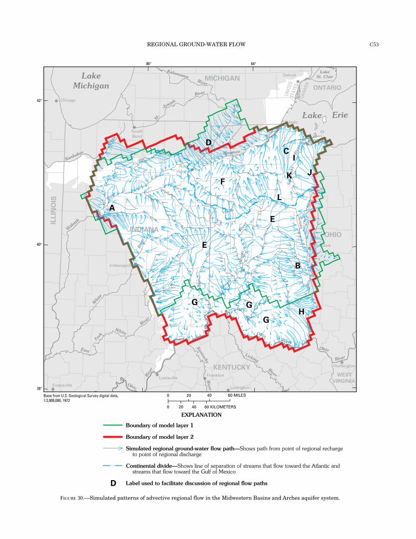
REGIONAL GROUND-WATER FLOW C53
84°86°
42°
40°
38°
Base from U.S. Geological Survey digital data,1:2,000,000, 1972
0 20
0 20 40 60 KILOMETERS
40 60 MILES
Lake Erie
Maumee
River
KalamazooRiver
St.
Joseph
River
San
dusk
yR
iver
Scio
to
River
Great
Mia
mi
Rive
r
OhioRiver
Ohio
Riv
er
Ohio
River
East
Fork
White
Whi
te
Riv
er
Wab
ash
River
Kankakee
River
River
Kentucky
River
Licking
River
LakeMichigan
LakeSt. Clair
Chicago
Indianapolis
Detroit
Columbus
Cincinnati
Toledo
Dayton
Evansville
Louisville
FortWayne
SouthBend
Frankfort
Lexington
Huntington
ILLIN
OIS
MICHIGAN
INDIANAOHIO
WEST
VIRGINIA
KENTUCKY
ONTARIO
UNIT
EDST
ATES
CAN
ADA
D
F
CI
JK
L
E
E
B
H
G G
G
A
EXPLANATION
Boundary of model layer 1
Boundary of model layer 2
Simulated regional ground-water flow path—Shows path from point of regional recharge to point of regional discharge
Continental divide—Shows line of separation of streams that flow toward the Atlantic and streams that flow toward the Gulf of Mexico
Label used to facilitate discussion of regional flow pathsD
FIGURE 30.—Simulated patterns of advective regional flow in the Midwestern Basins and Arches aquifer system.

REGIONAL AQUIFER-SYSTEM ANALYSIS—MIDWESTERN BASINS AND ARCHESC54
84°86°
42°
40°
38°
Base from U.S. Geological Survey digital data,1:2,000,000, 1972
0 20
0 20 40 60 KILOMETERS
40 60 MILES
Lake Erie
Maumee
River
KalamazooRiver
St.
Joseph
River
San
dusk
yR
iver
Scio
to
River
Great
Mia
mi
Rive
r
OhioRiver
Ohio
Riv
er
Ohio
River
East
Fork
White
Whi
te
Riv
er
Wab
ash
River
Kankakee
River
River
Kentucky
River
Licking
River
LakeMichigan
LakeSt. Clair
Chicago
Indianapolis
Detroit
Columbus
Cincinnati
Toledo
Dayton
Evansville
Louisville
FortWayne
SouthBend
Frankfort
Lexington
Huntington
ILLIN
OIS
MICHIGAN
INDIANAOHIO
WEST
VIRGINIA
KENTUCKY
ONTARIO
UNIT
EDST
ATES
CAN
ADA
EXPLANATION
Boundary of model layer 1
Discharge vector—Length of arrow shows relative magnitude and arrow points to resultant direction of horizontal flow in each model cell in layer 1
FIGURE 31.—Simulated relative magnitudes of horizontal regional flow in the Midwestern Basins and Arches aquifer system:(A) glacial deposits.
A

REGIONAL GROUND-WATER FLOW C55
84°86°
42°
40°
38°
Base from U.S. Geological Survey digital data,1:2,000,000, 1972
0 20
0 20 40 60 KILOMETERS
40 60 MILES
Lake Erie
Maumee
River
KalamazooRiver
St.
Joseph
River
San
dusk
yR
iver
Scio
to
River
Great
Mia
mi
Rive
r
OhioRiver
Ohio
Riv
er
Ohio
River
East
Fork
White
Whi
te
Riv
er
Wab
ash
River
Kankakee
River
River
Kentucky
River
Licking
River
LakeMichigan
LakeSt. Clair
Chicago
Indianapolis
Detroit
Columbus
Cincinnati
Toledo
Dayton
Evansville
Louisville
FortWayne
SouthBend
Frankfort
Lexington
Huntington
ILLIN
OIS
MICHIGAN
INDIANAOHIO
WEST
VIRGINIA
KENTUCKY
ONTARIO
UNIT
EDST
ATES
CAN
ADA
EXPLANATION
Boundary of model layer 2
Discharge vector—Length of arrow shows relative magnitude and arrow points to resultant direction of horizontal flow in each model cell in layer 2
FIGURE 31. Continued—Simulated relative magnitudes of horizontal regional flow in the Midwestern Basins and Arches aquifer system:(B) bedrock.
B

REGIONAL AQUIFER-SYSTEM ANALYSIS—MIDWESTERN BASINS AND ARCHESC56
consistent with the hypothesis that regional recharge to thispart of the aquifer system could be limited by the inability ofthe aquifer system to carry ground water away from the area.This area is largely coincident with the area of weak regionaldischarge (fig. 28).
Simulated discharge vectors indicate high magnitudes ofhorizontal regional flow in the carbonate-rock aquifer in theareas around the regional potentiometric highs (fig. 31B).High magnitudes of horizontal regional flow are also associ-ated with the downstream end of the Wabash and White Riv-ers, the margin of the Illinois (structural) Basin, the OhioRiver, an area west of the Scioto River, and the area east ofthe Sandusky River. Discharge vectors along part of the LakeErie shore indicate that the magnitude of horizontal regionalflow in the carbonate-rock aquifer in this area is fairly small.Ground-water flow may be predominantly vertical in this areabecause it is an area of regional ground-water discharge. Sim-ulated discharge vectors were computed for the upper weath-ered zone water-bearing unit, but the relative magnitudes offlow in this poorly permeable unit are so small that the vec-tors do not show up at the scale of figure 31B.
It should be noted that the discharge vectors show onlyrelative magnitudes of horizontal regional ground-water flowand do not indicate flow velocities. Additional information onthe effective porosity of the aquifers would be necessary tocompute flow velocities. Appropriate effective-porosity datafor fractured carbonate rock are difficult to obtain and werenot available for this investigation. Ground-water ages pre-sented in the following section, however, provide insight intoground-water residence times.
The calibrated final model was not used to simulatepotential effects of future pumpage on regional ground-waterflow in the aquifer system. Data on future pumpage needs atthe regional scale are not available, and any simulations offuture pumpage at this time would be contrived. It is notewor-thy, however, that only a small percentage of current pump-age is associated with the regional flow systems explicitlysimulated with this model. Therefore, more water associatedwith such regional flow systems almost certainly could beused. The quality of the ground water associated with someparts of the aquifer system, however, may limit its use.
GEOCHEMISTRY
Geochemical data were collected from the MidwesternBasins and Arches aquifer system to investigate the relationsamong ground-water chemistry, aquifer mineralogy, andpresent and past patterns of regional flow. The data include asynthesis of basic data from more than 1,300 ground-wateranalyses of water samples from the aquifer system, as well asdetailed chemical and isotopic analyses of ground water andaquifer material along general directions of regional flow. Theanalyses represent two hydrologic units (table 1) within the
Midwestern Basins and Arches aquifer system — aquiferswithin glacial deposits and the carbonate-rock aquifer — andwere obtained from records in the U.S. Geological Survey’sNational Water Information System (NWIS) data base; filesof the Indiana Department of Natural Resources, the OhioDepartment of Natural Resources, and the Ohio Environmen-tal Protection Agency; various published reports; and samplescollected as part of this investigation. The data were compiledand analyzed to investigate the ground-water chemistry of theaquifer system on a regional scale. Ground-water chemistryof subregional areas of the Midwestern Basins and Archesaquifer system is described in the following reports: in Ohio,by Ohio Department of Natural Resources, Division of Water(1970), Norris and Fidler (1973), Norris (1974), Deering andothers (1983), Breen and Dumouchelle (1991); and in Indi-ana, by Geosciences Research Associates, Inc. and PurdueUniversity, Water Resources Research Center (1980) andIndiana Department of Natural Resources (1988, 1990).Analyses of brines from rocks of Silurian and Devonian ageare found in Stout and others (1932), Lamborn (1952),Walker (1959), Stith (1979), Keller (1983) and Wilson andLong (1993a, b).
Data compiled from the literature and the available databases were selected on the basis of the following criteria: (1)major-ion concentrations (Ca, Mg, Na, Cl, SO4, and HCO3)were determined, (2) the analyses balanced electrochemicallywithin 10 percent and, (3) lithologies of the water-producingunits were determined. In cases where multiple analyses wereavailable for a well, the most recent analysis that met theabove criteria was selected. The dissolved-solids data formost of the analyses that were used in this report were calcu-lated by summing the concentrations of all major constituentsaccording to the method described in Fishman and Friedman(1989). Dissolved-solids concentrations for waters in the Illi-nois and Michigan Basins were estimated from borehole geo-physical data where available laboratory determinations weresparse (D.J. Schnoebelen, U.S. Geological Survey, writtencommun., 1993).
New data that were collected during this investigationinclude detailed chemical and isotopic analyses of groundwater from the aquifer system along general directions ofregional ground-water flow, as determined from the map ofthe potentiometric surface of the carbonate-rock aquifer (fig.12), and isotopic analyses of aquifer material collected fromcores of glacial deposits and carbonate rock. The locations ofthe ground-water and aquifer-material samples are shown infigure 32. At each sampling location along four transectsacross the aquifer system, ground-water samples were col-lected from the carbonate-rock aquifer, and, where possible,from a glacial aquifer. Sampling was restricted to existingdomestic wells or test wells; wells with short open intervalsin the deep parts of the aquifer were generally not available.At each sampling location, an attempt was made to samplethe deepest available well in the carbonate-rock aquifer in