buy it now: an analysis of the effects of buy prices in ... · buy it now: an analysis of the...
TRANSCRIPT
Buy it Now: An Analysis of the Effects of Buy Prices in Auction Listings
May 2015
Anthony Ding
Department of Economics
Stanford University Stanford, CA 94305
Under the direction of Professor Liran Einav
Abstract The rise of online auction platforms in the past decade has presented a wealth of new data and puzzling effects to researchers. New listing strategies and parameters created to give both sellers and bidder flexibility have also led the way for new types of listings. This paper explores the potential behavioral effects of simultaneously listing an auction with a fixed price option using data from eBay. It looks specifically at how the fixed price option—known as the Buy it Now (BIN) option on eBay—affects bidder behavior and how this translates into seller outcomes. It looks at (1) whether or not the BIN price has an effect on the final sale price of an auction, and (2) whether this effect can be attributed to anchoring. Two main results arise from this study. The first is that BIN prices have a positive effect on expected seller revenue, especially when the BIN price is more persistent and when the item is more unique. In the case of the former, this is caused by the higher probability of BIN exercise and in the later, this is caused in part by the pure existence of the BIN price. Second, bids anchor to the BIN price, which can help explain the mechanism through which final sale prices rise with the BIN price. This result is significant because in contrast to previous literature, it suggests that sellers might still benefit by setting a BIN option with effectively zero probability of exercise. Keywords: Internet auctions, online markets, anchoring, bidder behavior Acknowledgements: I would like to thank my advisor, Professor Liran Einav—without whom, this thesis would not be possible—for his support, encouragement, and patience. I would also like to thank Professor Marcelo Clerici-Arias for his assistance early in the process and the constant feedback throughout. Dr. Neel Sundaresan, who introduced me to the complexities of data analysis at eBay has my utmost gratitude. I also benefited greatly from comments from Dr. Peter Coles and Dr. Thomas Blake at eBay. Chiara Farronato and Michael Dinerstein helped immensely in the data collection process. Finally, I would like to thank my parents and friends whose understanding and encouragement helped more than they will ever know.
Ding 1
1. Introduction
In the first quarter of the 2015 fiscal year, online marketplace eBay helped transact
roughly $20.2 billion in gross merchandise volume, part of which came from 800 million
listings worldwide (eBay 10-Q 2015). Since introducing fixed price sales in 2002
(Wolverton 2002), eBay has steadily made moves emphasizing the fixed price format
over its traditional auction listings (Flynn 2008) and there has been growing evidence that
sellers have reacted to this, favoring the fixed price alternative to eBay’s traditional
auction listings (Einav, Farronato, Levin, and Sundaresan 2013). Of the 800 million
listings, roughly 160 million were some type of auction listing with the remaining 640
million making up fixed price sales (eBay 10-Q 2015).
Despite the shift towards fixed price listings, eBay has consistently allowed its
sellers additional layers of flexibility with the introduction of different listing strategies
and parameters. One such parameter is the “Buy it Now” (BIN) option.1 The BIN option
allows sellers to create an auction and fixed price hybrid listing and list an item as an
auction, while simultaneously posting a fixed price. This option allows potential bidders
to forego participating in the auction and, instead, purchase the item outright as if it were
a fixed price sale. While the BIN price itself is equivalent to a fixed price listing, the
focus of this paper will be on the effect of the BIN price in auction plus BIN hybrid
listings. In most cases of the auction plus BIN listing, once a valid bid has been
submitted, the BIN option disappears and the listing becomes a pure auction listing. The
exception to this behavior occurs in certain categories where eBay has implemented a
longer-lasting BIN option that persists until bidding has reached 50 percent of the BIN
!!!!!!!!!!!!!!!!!!!!!!!!!!!!!!!!!!!!!!!!!!!!!!!!!!!!!!!!1 While there are many names for this type of option and BIN is an eBay-specific term, for simplicity, this paper will refer to buy prices in general as BIN options.
Ding 2
price.2 Of the nearly 2.4 billion auction listings posted on eBay in the year 2014, roughly
19.7 percent were auction plus BIN hybrid listings.
What is interesting about the auction plus BIN listing is that, where a bidder in a
pure auction listing faces only one decision, his bid amount, the bidder in a hybrid
auction listing that currently has no bids must now weigh two related decisions: (1)
whether or not he should purchase the item at the BIN price and if not, (2) what he should
bid on the item. The existence of the hybrid BIN listing may thus affect bidder decisions
in ways that differ from a standard pure auction listing. Intuitively, we might hypothesize
that if the seller sets a BIN price higher than the average sale price of an item, he may
increase his expected revenue if bidders exercise the BIN price. In fact, it has been shown
both theoretically (Budish and Takeyama 2001; Mathews and Katzman 2006) and
empirically (Ackerberg, Hirano, and Shahriar 2006) that setting a high BIN price leads to
higher expected seller revenues. The mechanism through which this occurs is the exercise
of the BIN option by risk averse or impatient bidders who may decide that, instead of
taking an uncertain outcome by bidding in the auction, they would prefer to own the item
with certainty by taking the BIN price.
There are, however, two major dimensions to the BIN option: (1) whether or not it
exists, and (2) whether or not it is exercised. My goal in this paper is to explore whether
the existence of the BIN price and by extension, its magnitude, has an effect on bidder
behavior independent of its exercise and if so, how it does this. I focus specifically on the
effect of the BIN option in auction listings. In addition, I explore the effect of the BIN
price in various subgroups of listings on eBay. I look specifically at a subgroup of listings
that have a more persistent BIN option and a subgroup of listings where the items are !!!!!!!!!!!!!!!!!!!!!!!!!!!!!!!!!!!!!!!!!!!!!!!!!!!!!!!!2 See http://www2.ebay.com/aw/core/200710161010352.html
Ding 3
more unique and may not have an established or consistent market value and compare the
effects of the BIN option in these groups to a baseline group of listings that have the
standard BIN rules and more comparable items. To this end, I define three subgroups
within my data that contain: (1) listings in eBay-defined categories with a longer-lasting
BIN option, (2) listings in categories that have more unique and thus less comparable
items, such as antiques and collectibles, and (3) a baseline group that includes all listings
not in any of the other two categories. To clarify, groups (2) and (3) have the standard
BIN listing rules and (1) has a more persistent BIN. Groups (1) and (2) tend to have more
comparable and ubiquitous items and group (3) has more unique items. Thus there are
two dimensions of variation among my groups: BIN duration and item comparability.
The empirical strategy I take advantage of follows the matched listings approach
developed by Elfenbein, Fisman, and McManus (2012) and modified by Einav, Kuchler,
Levin, and Sundaresan (2015). This particular strategy allows me to compare identical
listings by the same seller that have variation in the listing parameters. In particular, I
focus on variation in the BIN parameter, looking at its effects on bidding behavior and by
extension, its effect on seller outcomes. The key link that I attempt to establish in this
paper is one between the BIN price and the final sale price. In particular, I attempt to
show that the BIN option affects the final sale price and that the relationship is positive,
whereby setting a higher BIN price can results in higher expected seller revenue. More
specifically, I aim to identify an existence effect of the BIN price separate from its
exercise effect. To do this, I split my analysis into three major steps.
In the first step of my analysis, I explore the effect of the BIN option on the final
price while including the effect of sales completed via BIN exercise. I find that at the
Ding 4
highest quartile, setting a BIN option can increase final prices anywhere from 7-13
percent depending on the group the listing is in, where the final prices of items with a
more persistent BIN price and with more unique characteristics are affected more
substantially by a high BIN price. When I isolate the existence effect of the BIN by
excluding listings where the item is sold via the BIN option, I find that this positive effect
persists and is consistently significant when the BIN is set in the highest quartile, where
the effect ranges from 3-10 percent. I find that the effect is strongest when the item has an
uncertain value. Comparing the two regressions, I confirm that the BIN price affects final
prices through both its exercise and its existence. The overall effect of the BIN price is
greater when the BIN is more persistent and when the underlying value of the item is
more uncertain. However, in the more persistent BIN category, BIN exercise contributes
more to the effect of the BIN price on the final sales price due to the increased duration of
BIN availability. In the listings of items with uncertain values, it is the existence effect of
the BIN price that contributes more significantly to the higher final sales price due in part
to behavioral anchoring to the BIN option. Thus, while the overall effect of the BIN price
on final prices is similarly high in the longer BIN and more unique item groups compared
to the base group, the composition of the effect differs: in the longer BIN category, the
exercise effect of the BIN price dominates and in the uncertain value category, the
existence effect of the BIN price dominates.
Next, I explore the channels through which the effect of the BIN option might
manifest by looking at its effect on first and second bids. I find evidence that the first bid
anchors to the BIN price, but only consistently in the highest quartile. The effect ranges
from 11-21 percent depending on the group. I find that the anchoring effect is highest in
Ding 5
the group of items with uncertain values. I find, surprisingly, that second bids also rise
with the BIN price. The effect on the second bid ranges from 11-21 percent and the effect
is similarly largest in listings that I define as having uncertain values. This suggests that
while the BIN price disappears after the first bid in certain categories, it could be that all
or most of the bidders in the auction are affected by the BIN price and that while a valid
bid can make the BIN option disappear, it’s anchoring effect is not substantially
diminished because most subsequent bidders were aware of the BIN option prior to its
removal. It also provides some justification for how the existence of the BIN price could
affect final sale prices through the anchoring of bids. I also look at the potential effect of
the BIN price on the number of bids submitted as a proxy for bidder interest or
aggression. I find significant positive effects in the base group and significant negative
effects in the longer BIN group with no significant effect in the uncertain value group.
The effect of the BIN price on the number of bids is overall not very conclusive.
Finally, I run a set of regressions to show the effect of the first bid and the bid
count on the final price. I find that this effect is highly significant across all three groups.
From these results, I draw the conclusion that part of the existence effect of the BIN price
on the final sale price occurs through an anchoring effect. While the bid count does have
a significant effect on the final price, the BIN price only has a significant effect on bid
count in the base group.
The rest of this paper will proceed as follows. Section 2 will give some
background information about eBay and review some relevant literature. Section 3 will
outline the source of the data, the filtering process used in this paper, and the matched
listing strategy. Section 4 will cover the empirical strategy I rely on and address some
Ding 6
important issues of endogeneity and selection. Section 5 will present the results and
discuss them in context of previous literature. Section 6 will conclude with a summary
and synthesis of the results and attempt to offer some practical advice for sellers as well
as some potential directions for future study motivated by the results obtained.
2. Background & Literature Review
In general, there has been a substantial amount of literature on eBay auctions,3 perhaps
because of the wealth of data and insights eBay offers to researchers. I will begin by
giving a quick overview of the bidding process on eBay. Next, I will summarize some of
the main results of previous studies as they pertain to buyer behavior in eBay auctions. I
will then discuss studies and research that has looked specifically at the effects of the
BIN option. I will also cover some preliminary research that has looked at behavioral
influences in auctions. Finally, I will give a brief overview of the contributions this paper
attempts to make to the existing literature and knowledge base.
Ebay operates its auctions via a mechanism called proxy bidding. Bidders are
asked to input their maximum willingness-to-pay (WTP) and the proxy bidder software
will bid automatically for the user up to their stated WTP. If the current bidder is not the
highest bidder, the proxy bidder will look at the current price and will continue to bid the
current price plus some small bid increment4 so long as this total amount is below the
user’s WTP. The user’s stated WTP is never revealed but the bid that the proxy bidder
places on his behalf is. Note that this is effectively a second-price sealed-bid auction. The
!!!!!!!!!!!!!!!!!!!!!!!!!!!!!!!!!!!!!!!!!!!!!!!!!!!!!!!!3 For a comprehensive summary on research on eBay auctions and online auctions in general, readers are directed to Lucking-Reilly (2000), Hasker and Sickles (2001), and Bajari and Hortaçsu (2004). 4 This amount is a function of the current high price and ranges from $0.05 to $100.

Ding 7
winner of the auction wins when any other bidder cannot match his bid. The final price of
the auction is thus equivalent to the second-highest stated WTP plus the bid increment.
Figure 1 gives an example of a typical auction listing with a BIN price. Note that if the
BIN option does exist, the price is highly visible to current bidders and the option to
exercise it mirrors the option to place a bid.
2.1 General Determinants of Bidder Behavior and Seller Revenue on eBay
Because eBay offers sellers many options to customize their listings, there are a
large variety of listing types a given bidder can expect to run into while shopping on
eBay. The first decision sellers must make is the broad choice of listing format, but even
after that, sellers are given the choice of setting reserve prices, secret reserves, and
shipping prices. Additionally, certain seller characteristics that are visible on listing pages
such as seller reputation may also influence bidder behavior.
Ariely and Simonson (2003) study auction entry decisions through auctions for
Rose Bowl tickets and find that the final price of an auction is significantly and positively
influenced by the start price, total number of bids, and total number of bidders. Using
eBay data on coin auctions, Bajari and Hortaçsu (2003) explore the effects and
interactions of both public and private reserve prices.5 They find that higher public
reserve prices are correlated negatively with the total number of bidders who bid in an
auction. They also find that in auctions with at least two bidders, an additional bidder
increases auction revenue by 5.5 percent on average. Conditional on bidder entry, they
find that higher public reserve prices lead to higher seller revenue in auctions with more
!!!!!!!!!!!!!!!!!!!!!!!!!!!!!!!!!!!!!!!!!!!!!!!!!!!!!!!!5 In general, as it relates to eBay auctions, the terms minimum bid, starting price, and public reserve are interchangeable. All three can be seen as the seller’s own bid that is public and starts off the auction. The private reserve is the same except it is never made public to bidders.
Ding 8
than two bidders. They find that setting a private reserve price negatively impacts seller
revenue by nearly 13 percent across all auctions.
Katkar and Lucking-Reilly (2000) carry out a field experiment by auctioning off
Pokémon cards in matched pairs, with one listing including a public reserve and another
including a secret reserve at the same level. They find that setting a private reserve price
decreases the probability of sale significantly. In addition, they note that setting a private
reserve price decreases the number of bidders and setting a public reserve price in place
of a private reserve price of the same magnitude results in higher seller revenue by
roughly 90 percent.
Lucking-Reilly, Bryan, Prasad, and Reeves (2007) collect data on eBay auctions
of collectible US pennies and find that seller reputation, reserve prices, and auction
duration have a significant effect on auction outcomes and prices. They find that a 1
percent increase in positive feedback scores for sellers corresponds to a 0.03 percent
increase in seller revenue and that the same decrease in seller feedback corresponds to a
0.11 percent decrease in seller revenue. In addition, they find that setting an auction
duration of seven days raises revenue by 24 percent on average compared to a duration of
three days and setting a ten-day auction duration raises revenue by 42 percent on average.
They also find that setting a public reserve price or a private reserve price increase seller
revenue but that the increase from a public reserve price is not significant whereas setting
a private reserve price increases seller revenue by 15 percent on average.
Hossain and Morgan (2006) auction music CDs and Xbox games and find that in
the case of Xbox games and while holding constant the total cost, lower public reserve
prices and higher shipping costs yielded higher revenues than higher public reserve prices
Ding 9
and lower shipping costs. They explain this effect as either a combination of loss aversion
and mental accounting on the part of the bidder, or disregard for shipping costs when
bidding. Einav et al. (2015) also look at shipping costs and find that a $1 increase in
shipping fees corresponds to a $0.82 decrease in the final sale price, suggesting that
bidders do not fully take the shipping fee into account.
2.2 BIN Prices and eBay Auctions
There has additionally been a fairly substantial amount of literature on the BIN
option and its effect on bidder behavior and in the following subsection, I split a sample
of the existing literature into theoretical discussions of the BIN option and empirical
studies that have been conducted on BIN options which have generally supported the
theoretical framework.
Budish and Takeymama (2001) look specifically at permanent BIN options and
show that, in a two-bidder model, it may be theoretically sound for a seller to set a BIN
price despite the fact that it is functionally an upper limit on the amount of revenue a
seller can obtain. In particular, they note that if bidders a risk averse, they may see the
BIN price as a form of insurance and thus, setting a buy price may allow sellers to
increase expected revenue. Reynolds and Wooders (2009) further extend this result to
instances with temporary BIN prices—consistent with the BIN format on eBay—and find
that, while both temporary and permanent BIN prices lead to higher expected revenues
compared to a pure auction listing, permanent BIN prices are more effective relative to
temporary BIN prices. Matthews and Katzman (2006) consider the opposite case where
bidders are risk neutral and sellers are risk averse and find that sellers will still choose a
Ding 10
BIN price with a positive probability of exercise. Hidvégi, Wang, and Whinston (2006)
find that setting a BIN option can increase expected utility for both buyers and sellers
when either are risk averse but that the temporary BIN price is less effective than the
permanent BIN price.
Mathews (2004) additionally makes the case for impatience on the side of the
bidders and shows that sellers who face impatient bidders will choose a BIN price that
will be exercised with positive probability. Bose and Daripa (2009) also propose an
alternative explanation for the success of BIN options and determine that the optimal
sales mechanism for a seller constitutes some combination of a fixed price option and an
auction listing, which allows the seller an additional dimension of price discrimination.
They additionally show that a temporary BIN option corresponds with the optimal selling
mechanism while a permanent BIN option does not.
In addition to theoretical interest in the BIN option, there have been a number of
empirical studies that have explored the effects of the BIN option on bidder behavior and
seller outcomes. Durham, Roelofs, and Standifird (2004) study the interaction between
eBay’s BIN option and seller reputation through the use of controlled auctions with BIN
variation posted by the authors themselves and through listed auctions with BIN variation
posted by sellers on eBay. They find that the BIN option tends to be used more frequently
by high reputation sellers and that the probability of a BIN price exercise increases with
the reputation of the seller and with the decrease in BIN price. Anderson, Friedman,
Milam, and Singh (2008) find additional evidence to support the positive effect of
reputation on the probability of BIN price exercise. They also find that while the choice
of a BIN option does not have statistically significant effect on the final sale price,
Ding 11
conditional on having a BIN option, the final sale price increases with the BIN price
regardless of whether or not the BIN price is exercised.
Ackerberg, Hirano, and Shahriar (2006) collect information from eBay on
auctions of Dell laptops and find that, without controlling for the level of the BIN price,
having a BIN price contributes to an average increase in expected revenue for the seller
of roughly $29. Regressing expected revenue on the BIN price, they find that revenues
increase by roughly $0.07 per dollar increase in the BIN price. These regressions do not
control for whether the sale is a BIN sale or an auction sale however and capture the
combined revenue effect of the both the pure existence of the BIN price and its exercise.
Shahriar and Wooders (2011) conduct an experiment on the effect of temporary
BIN prices in cases where bidders have private values and common values and finds that,
consistent with theory, with private values, seller revenue is significantly higher in
auctions with a temporary BIN price and in fact, that the lowest revenue achieved with
the BIN option was greater than the highest revenue achieved without the BIN option. In
the case of common values, they find results contrary to the theory; namely, that setting a
BIN price does not hurt expected seller revenue. They account for this inconsistent
finding with a behavioral model of naïve bidding.
Einav et al. (2015) study a wide variety of parameters and their effects, but in the
context of BIN prices, they find that setting a high BIN price relative to the reference
price of a particular item leads to higher seller revenue for the seller. They also test for
the effect of the BIN price if it is not exercised by looking at how different levels of the
BIN price affect the probability of sale. They find virtually no difference in the
probability of sale at different sale prices with different levels of the BIN price.
Ding 12
2.3 Some Evidence of Anchoring in Auctions
While the result that sellers can increase expected revenues by setting BIN prices
and the mechanism through which this occurs—exercise of the BIN option—has been
robustly established in theory and in practice, there has been a relatively small amount of
literature that has explored potential behavioral effects in auctions. These studies suggest
an alternative effect of BIN price through some form of anchoring.
Beggs and Graddy (2009) give evidence of an anchoring effect in a non-lab
setting and focus on art auctions. They use data from art auctions of Impressionist art sold
in London and New York and find that a 10 percent increase in the previous sale price
and the predicted sale price leads to a 6.2 to 8.5 percent increase in the actual sale price.
Hong, Kremer, Kubik, Mei, and Moses (2015) study the effects of the ordering in
sequential auctions, focusing of art auctions of Impressionist and Modern art held by
Sotheby’s and Christie’s. They find that in weeks where more expensive items are
auctioned early in the week, the weekly sale premium is 21 percent higher than the
average sale premium. Both of these studies suggest that final sales prices might be
susceptible to anchoring onto other established prices.
There has also been limited research on the effect of anchoring as it related to
BIN prices. Dodonova and Khoroshilov (2004) provide some evidence of anchoring in
online auctions. Using auction listings from Bidz.com, they take advantage of the same
seller posting multiple listings with different BIN prices. They find that variance in the
BIN price significantly affects the final sale price in a positive direction. Their study,
however, focuses on the use of a permanent BIN price and it is unclear whether they
control for exercise of the BIN price or not. In addition, while their results are interesting
Ding 13
and greatly motivate further study of the potential anchoring effects of the BIN option,
the small sample size they use—an average of roughly 27 observations across all three
items—makes it difficult to draw any broad conclusions.
2.4 Contribution to Existing Literature
Thus in conducting this analysis, I attempt to add to the existing literature in three
ways. First, I use a rich dataset on auction listings and parameters collected from eBay.
Some previous studies that have looked at eBay auction behavior have obtained data by
scraping data or conducting experimenter listings and are generally limited by the
completeness of the data used and the sample size of observations. The second way I
attempt to add to the literature is by additionally exploring the behavioral effect of the
BIN option and by looking at how this effect changes in different groups. I define these
groups to test specifically for the differential effects of the BIN price when there is
variation in the duration of the BIN price and when items become more unique and less
comparable. Finally, I apply the strategy of matched listings used in Einav et al. (2015) to
studying the effects of BIN listings across a broader range of products and categories,
where previous papers have focused on specific categories or products, making broader
and comparative conclusions more difficult.
3. Data
What follows is a brief description of the general steps I take to create my final dataset.
The steps are then described in more detail in the following paragraphs. I first impose a
group of limits on the initial collection to manage the size of my dataset as well as control
Ding 14
for the potential confounding effects of different listing parameters outlined above in the
discussion of previous literature (Table 1.1). I then construct matched sets from this
group of listings by matching those with the same seller, category, and listing title. After
this, I normalize the BIN prices by a reference price for comparability and drop those
listings without a reference price (Table 1.2). Next, I drop all matched sets that do not
have variation in the BIN option or BIN price (Table 1.3). Finally, I trim this intermediate
dataset by dropping all outliers. This ultimately gets me to my baseline data set (Table
1.4). What follows is a brief justification of each step in my data narrowing process.
3.1 Collecting Auction Listings
In collecting the initial set auction listings, I focus on listings in the year 2014 and
I limit the auctions I collect to those whose start- and end-dates fall within the date range,
January 1, 2014 to December 31, 2014 to ensure that I am not cutting any auctions short.
I exclude eBay Motors and Real Estate listings as those categories contain their own
unique listing rules that aren’t consistent with rule in the other categories. I limit my data
collection to only single-quantity listings to control for situations in which there may be
substitutability or complementarity among multiple units (Milgrom and Weber 2004). In
addition, I limit the listings I collect to those on the US eBay website and those listed in
US dollars in order to control for any exchange rate issues and pass-through effects. In
light of the effects outlined above in the discussion of previous literature, I also limit my
sample to listings with no reserve price and free shipping. In addition to allowing me to
control for the effects of reserve prices and shipping fees, this limitation also helps
control the size of my dataset. In order to ensure that start prices are not affecting bidding
Ding 15
behavior or otherwise influencing the level of first bids, I further limit my initial data
collection to listings with start prices that are equal to or under $1. I also limit my results
to listings of new items to ensure that bidders are not responding to the condition of an
item. I collect all first bids on listings as well as second bids if they exist. The initial
collection results in a sample of roughly 45.4 million listings of which 42.8 million are
unique.6 Summary statistics for this first pass are included in Table 1.1.
3.2 Constructing Matched Listings and Finding Reference Prices
After the initial collection, I rely on the same matched listings strategy employed
by Einav et al. (2015) and I group listings by seller ID, category, and auction title. This
strategy is preferable to regressing over the entire set of listings as it allows for finer
control over the regression and takes advantage of the fact that sellers may experiment by
listing the same item with variations in different parameters. It also allows me to control
for the effects of seller characteristics and potentially different bidding behavior
depending on the specific item being listed. Unlike Einav et al. (2015), however, I do not
match on listing subtitles. Given that I eventually drop all matched listing sets that do not
have any variation in the BIN price, I end up losing a sizeable amount of the data I have
collected. Thus, I attempt to maintain the largest baseline sample while also keeping the
matched listings accurate. While there may be variation in subtitles even when seller ID,
category, and auction title are matched, I make the assumption that this variation does not
significantly affect bidding behavior.
Because assessing the magnitude of a BIN price does not make sense unless
!!!!!!!!!!!!!!!!!!!!!!!!!!!!!!!!!!!!!!!!!!!!!!!!!!!!!!!!6 The duplication of observations occurs because I also collect second bids. The fact that less than half of the observations are duplicates is the result of not all listings having second bids. In particular, a standard auction plus BIN listing that ends via BIN exercise will not have a second bid.
Ding 16
compared against some reference price for a given item—for example, a $10 BIN price
on an item that usually sells for $1 is very different from a $10 BIN price on an item that
usually sells for $10—I follow Einav et al. (2015) and normalize BIN amounts by a
reference price for each matched set. In order to develop an estimate of the reference
price for a particular matched set, I use the average of all successful fixed price sales of a
particular item in the year 2014 as a proxy. To construct this average, I collect additional
data from eBay on fixed price sales conditional on success and construct matched listings
with the same method as I use for the auction data. Within these matched listings, I
average the sale price and collapse the sets into a single record that maps a unique
combination of seller ID, category, and auction title to an average fixed price7—the
reference price. Finally, I merge this mapping onto the auction data obtained earlier and
define normalized amounts as amounts divided by the average fixed price associated with
each set of matched listings. Because not all sets have corresponding fixed price sales, I
drop those matched sets that do not have any fixed price sales. See Table 1.2 for
summary statistics.
3.3 Isolating Matched Sets with BIN Variation
Once I obtain these sets of matched listings, I drop those sets in which there is
only one listing as the point of constructing the sets in the first place is to look at
variation within the sets. I also drop all sets with no BIN variation. BIN variation can
refer to changes in the existence of the BIN price or changes in the level of the BIN price
conditional on existence. I qualify both of these as BIN variation and drop sets in which
!!!!!!!!!!!!!!!!!!!!!!!!!!!!!!!!!!!!!!!!!!!!!!!!!!!!!!!!7 While I refer to this as the average fixed price of an item, note that because I also generate matched sets for the fixed price sales, this amount is really the average fixed price of a particular item listed in a particular category and being sold by a particular seller.
Ding 17
there is no BIN variation at all. Results after listings with no BIN variation are dropped
are shown in Table 1.3.
3.4 Final Baseline Dataset and Discussion
Finally, I cut out all outliers, which I define to be the top and bottom 1 percent of
observations by normalized final sales price—the final sales price divided by the average
fixed price of an item. The reason I classify outliers by the normalized sale price is that it
allows me to simultaneously consider outlier data in the fixed price listings and outlier
data in the auction price listings; large deviations between the two would result in either
abnormally large or abnormally small normalized final sale prices depending on the
direction of deviation. This gives me the final baseline dataset, which consists of 174,983
listings that make up 10,460 matched sets (see Table 1.4). By virtue of the restrictions I
place on my dataset, all of the listings in my baseline dataset happen to result in
successful sales. The only variation in the sales then is whether the sale is completed via
auction or via BIN exercise.
Each of the matched sets has an average of 16.73 listings with a minimum of two
and a maximum of 953 listings8 which gives me some confidence that there are enough
listings within each matched set to make within-set comparisons. The two most popular
categories by far are Jewelry & Watches and Cell Phones & Accessories, respectively
representing 37.9 and 24.5 percent of the sample, followed far behind by Clothing, Shoes,
& Accessories, which makes up 6.9 percent of the listings. In the construction of the
baseline dataset, I also define three subgroups. The first subgroup is defined by eBay and
includes categories in which the BIN price persists until the current price reaches 50 !!!!!!!!!!!!!!!!!!!!!!!!!!!!!!!!!!!!!!!!!!!!!!!!!!!!!!!!8 This particular seller was selling screen protectors for the iPhone 5 / 5S.

Ding 18
percent of the BIN price. I define these listings to be in the “Longer BIN” subgroup. The
second group is the “Uncertain Value” group and is less rigorously defined. The
motivation behind the creation of this group is to explore the hypothesis that bidders on
items that have less-established market values may be more susceptible to external
suggestions and anchors such as the BIN price. The categories I include within this
subgroup are: Antiques; Collectibles; Art; Stamps; Coins & Paper Money; Entertainment
Memorabilia; Sports Memorabilia, Cards & Fan Shop. While this category could be
constructed in a more thorough manner,9 the included categories seem fairly reasonable.
Summary statistics by group are shown in Table 2.
Note that by definition, when I construct matched sets, I necessarily drop items
that tend to be more unique, those that may not have any fixed price sales, and those that
may have very few listings and variation within those listings. The top panel in Figure 2
shows the breakdown of listings into the three groups that I define and as expected, the
Uncertain Value group has significantly less listings than the first two groups. While this
is an unfortunate tradeoff of using the matched listings approach, the Uncertain Value
group does still does have a fairly large number of listings in absolute terms.
The bottom panel in Figure 2 shows the breakdown in BIN exercise by group. As
we might expect, there is a significantly higher percentage of listings where the BIN price
is exercised in the Longer BIN group. Intuitively, the longer the BIN price is available,
the higher the chance that a bidder will come along who is willing to purchase the item
outright at the BIN price. In the Base and Uncertain Value groups, the proportion of BIN
!!!!!!!!!!!!!!!!!!!!!!!!!!!!!!!!!!!!!!!!!!!!!!!!!!!!!!!!9 Ideally, I would define “unique” items as those with a number of auction and fixed price listings below a certain threshold instead of broadly defining them via category. This would also require that I define such items before the filtering process as I pre-select for items with a trivial (<$1) start price and no reserve price; it could be that certain items are more likely to have higher start prices or reserve prices.
Ding 19
exercise is relatively consistent.
4. Methodology & Empirical Strategy
The data that I collect is organized into matched sets that have within-set variation in the
BIN option. This particular organization lends itself easily to fixed-effects regressions.
These regressions are ideal in that they allow me to control for effects that are invariant
across listings within the same set. Translated into the specific context of my data, this
allows me to control for any effects that may result from listings by a particular seller of a
particular item in a particular category.
To begin to motivate the regressions I run and to ensure that there is an effect to
study in the first place, I start by breaking the BIN price into four quartiles. I construct
the quartiles on the normalized BIN price, which I define as the absolute BIN price
divided by the average fixed price of the item. This lends itself to easier interpretation
and comparability of the BIN price. We can thus view a normalized BIN price of 1 to be
a fairly priced BIN, a normalized BIN price less than 1 to be an underpriced BIN, and a
normalized BIN price above 1 to be an overpriced BIN. The reason I create indicators for
the BIN price by quartile instead of regressing on the absolute price is that the
interpretation of any anchoring effect may make more sense by quartile. While we might
not expect a $1 change in BIN price to affect bidder behavior on the same item, a BIN
price set two times greater than the reference value may very well cause a change in
bidding behavior. The specific cut points are outlined in Table 3. As in Einav et al.
(2015), I find that, regressing the probability of BIN exercise on an indicator of the BIN
price in each quartile, the probability of a sale via the BIN option decreases with the level

Ding 20
of the normalized BIN price (Figure 3). The result is intuitive and we can imagine that it
is possible for the seller to set a BIN price that is so high that no one would exercise it.
In order to better understand the dynamics this effect, I define an indicator
variable that equals 1 if the bidder “overpays” for an item and 0 otherwise. I define
overpaying as a sale where the normalized final sale price is greater than 1. This
corresponds with a final price that is greater than the average fixed price of the item. I
then regress the probability of overpaying on the BIN price both including BIN exercise
sales and excluding BIN exercise sales (Figure 3). The results are rather surprising as,
while the probability of BIN exercise decreases with higher BIN price levels, the
probability of overpaying rises with the BIN price level. When we include BIN sales, this
effect seems readily explainable if there are still enough BIN sales at higher BIN prices to
increase the average expected seller revenue. However, operating under the assumption
that the BIN exercise is the only channel through which the BIN price has an effect on
the final sale price, we would expect that by excluding BIN exercise sales, the probability
of overpaying should be relatively constant across each BIN quartile. The fact that this is
not what I observe seems to indicate that the BIN exercise is not the only mechanism
through which expected seller revenue increases with the addition of the BIN option. This
is the motivation behind exploring the potential anchoring effects of the BIN option that
operate through BIN existence as opposed to exercise.
4.1 Empirical Strategy
To further develop this idea, I proceed by regressing the final sale price on the
existence of the BIN option broken down into quartiles in the form:

Ding 21
(1)
In the above specification, !! represents the fixed effect of being in a particular matched
set and !!" is a vector of indicator variables for the BIN option in each quartile. The
omitted indicator is an indicator for listings without a BIN option and hence the estimated
effects are relative to listings with no BIN option. I run this regression twice. The first
time is the unconditioned run where I allow for the effect of BIN exercise. Running the
regression a second time, I exclude all listings that sold via the BIN option exercise. This
allows me to compare the overall effect of the BIN option including BIN exercise with
the residual effect of the BIN option that cannot be explained through BIN exercise. The
interpretation of the ! coefficient is thus the existence and exercise effect of the BIN
price in the first set of regressions and captures the existence effect of the BIN price in
the second set of regressions. It may not be proper to take the ! in the regression as the
pure existence effect. While this issue is discussed in more detail in section 4.2, the core
issue is that the BIN option is likely to be exercised with higher probability at lower BIN
prices. Hence, exclusion of BIN sales creates a less-balanced sample, which could
overstate the effect of the BIN price on bids. For purposes of interpretation, I also look at
the above regression and replace !!" with the log of the BIN amount. This allows me to
interpret the effect of a percentage increase of the BIN amount on the final sale price.
This regression unfortunately also suffers from the same type of selection bias. When the
BIN option is not exercised, we can think of the group of subsequent bidders as a
subsample of the full group of bidders whose valuations are capped at the BIN price.10
!!!!!!!!!!!!!!!!!!!!!!!!!!!!!!!!!!!!!!!!!!!!!!!!!!!!!!!!10 This idea is connected to the two-step decision process described in the introduction. The general assumption is if the bidder is bidding on the item as opposed to exercising the BIN price, his WTP for the item is by definition under the BIN price or else he would have taken the BIN price.
log(Yit) = ↵i + �Xit + "it
Ding 22
Thus, at higher BIN prices, the distribution of first bidders on auction listings will
necessarily include bidders with higher valuations.
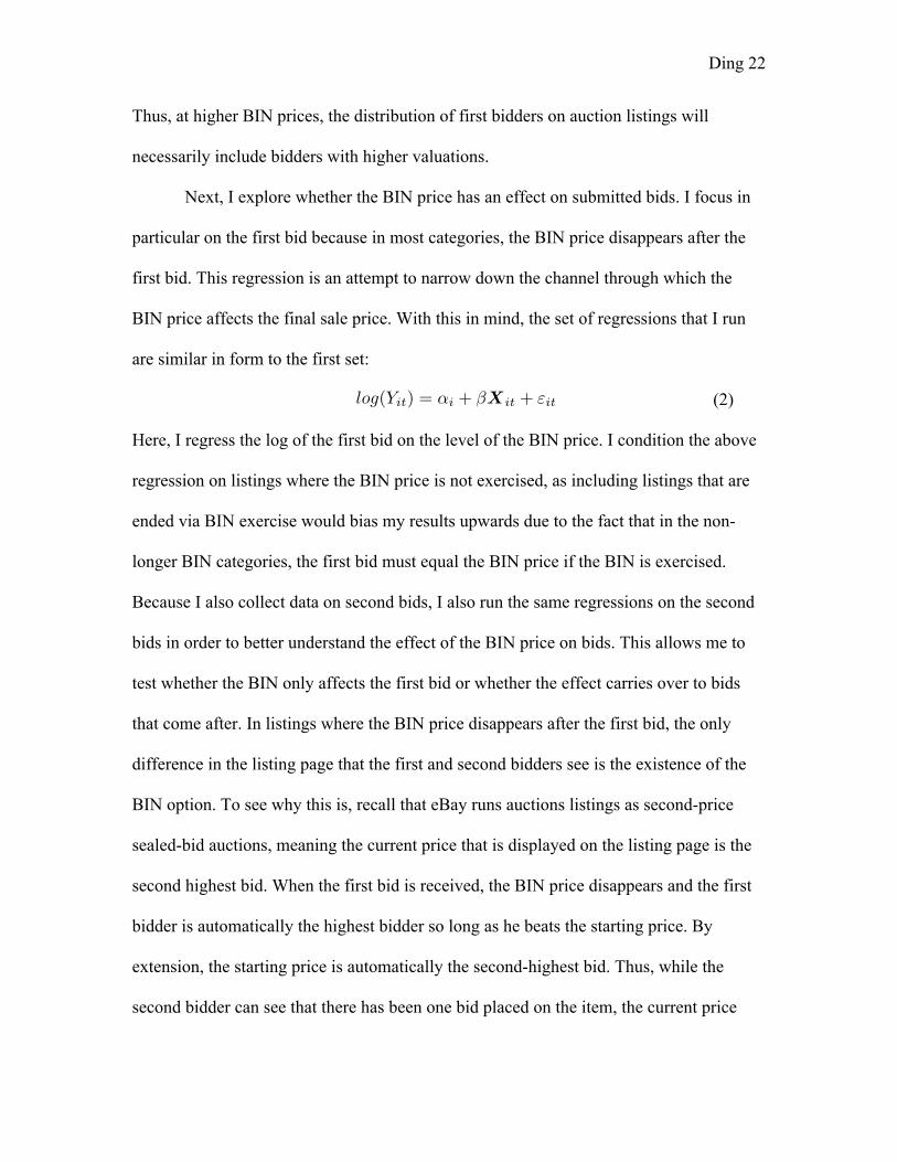
Next, I explore whether the BIN price has an effect on submitted bids. I focus in
particular on the first bid because in most categories, the BIN price disappears after the
first bid. This regression is an attempt to narrow down the channel through which the
BIN price affects the final sale price. With this in mind, the set of regressions that I run
are similar in form to the first set:
(2)
Here, I regress the log of the first bid on the level of the BIN price. I condition the above
regression on listings where the BIN price is not exercised, as including listings that are
ended via BIN exercise would bias my results upwards due to the fact that in the non-
longer BIN categories, the first bid must equal the BIN price if the BIN is exercised.
Because I also collect data on second bids, I also run the same regressions on the second
bids in order to better understand the effect of the BIN price on bids. This allows me to
test whether the BIN only affects the first bid or whether the effect carries over to bids
that come after. In listings where the BIN price disappears after the first bid, the only
difference in the listing page that the first and second bidders see is the existence of the
BIN option. To see why this is, recall that eBay runs auctions listings as second-price
sealed-bid auctions, meaning the current price that is displayed on the listing page is the
second highest bid. When the first bid is received, the BIN price disappears and the first
bidder is automatically the highest bidder so long as he beats the starting price. By
extension, the starting price is automatically the second-highest bid. Thus, while the
second bidder can see that there has been one bid placed on the item, the current price
log(Yit) = ↵i + �Xit + "it
Ding 23
will remain the same and he will only see that the first bidder bid the current price and
will not be able to get a sense of the first bidder’s WTP. Note that we should still be
cognizant of the possible selection bias in this case, which may muddle the interpretation
of the ! coefficient.
I also consider the possibility that the number of bids received might positively
affect that sale price of an item at auction. In this case, I take the bid count to be some
proxy of bidder interest or bidding aggression. Holding the item and first bid constant, it
could be that a greater amount of interest or more aggressive bidding might lead to higher
final sales prices. This idea is confirmed by Ariely and Simonson (2003). With this in
mind, I test to see if the BIN price has an effect on the number of bids submitted on a
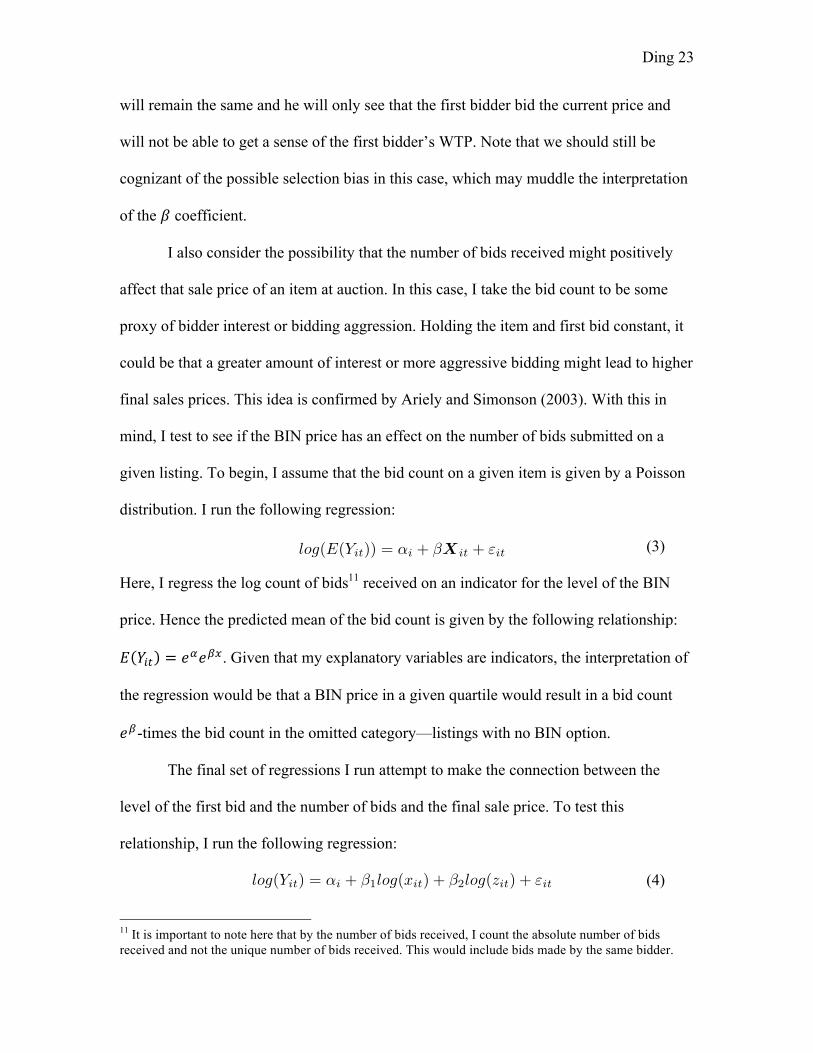
given listing. To begin, I assume that the bid count on a given item is given by a Poisson
distribution. I run the following regression:
(3)
Here, I regress the log count of bids11 received on an indicator for the level of the BIN
price. Hence the predicted mean of the bid count is given by the following relationship:
! !!" = !!!!". Given that my explanatory variables are indicators, the interpretation of
the regression would be that a BIN price in a given quartile would result in a bid count
!!-times the bid count in the omitted category—listings with no BIN option.
The final set of regressions I run attempt to make the connection between the
level of the first bid and the number of bids and the final sale price. To test this
relationship, I run the following regression:
(4)
!!!!!!!!!!!!!!!!!!!!!!!!!!!!!!!!!!!!!!!!!!!!!!!!!!!!!!!!11 It is important to note here that by the number of bids received, I count the absolute number of bids received and not the unique number of bids received. This would include bids made by the same bidder.
log(E(Yit)) = ↵i + �Xit + "it
log(Yit) = ↵i + �1log(xit) + �2log(zit) + "it
Ding 24
Here, I regress the log of the final sale price on the log of the level of the first bid and the
log of the number of bids received. The motivation behind this regression is to establish a
link between the first bid and the number of bids and the final sale price. In particular, if
the BIN option does affect first bids and bid counts and the first bid and bid counts affect
the final sale price, this allows me to consider first bids and the number of bids as
possible channels through which the existence of the BIN option might affect the final
sale price.
4.2 Addressing Endogeneity and Selection Bias
An important caveat to consider is that the matched sets I create are drawn from
the entire year. In particular, I do not cluster my matched sets so that all listings are from
the same month. The issue with this is that I cannot control for items that may be more
prone to seasonal variation in demand. Take, for example, a Thomas Kinkade “Christmas
on Main Street” tapestry—an item in one particular matched set. This item was listed and
sold in both June and October. We might expect that because this is a seasonal item,
increased demand in the months leading up to the Christmas season may cause the item
to sell for more and in fact, in my data, the item sold in October sold for 18 percent more
than the exact same item sold for in June. While this is not a perfect example, it illustrates
a potential source of endogeneity in my model. To help address this concern, I look at
variation in listing month within the matched sets and the results show that the average
variation is around one month. This gives me a sense that most of the listings in my
matched sets are not too widely dispersed. Even then, there is some evidence that the

Ding 25
effect of clustering listings may not change the results significantly.12 However, to
properly interpret the results, we must take these concerns into consideration.
A more concerning issue is the potential selection bias that arises from comparing
bids at varying levels of the BIN price and conditioning on listings that do not sell via
BIN exercise. To see this, consider the following example of a particular matched set, !,
with two listings !! and !!, where both listings have a BIN option but the BIN option in
!! is set at $10 and the BIN option in !! is set at $20. Let us consider a three-bidder
model where the distribution of bidder valuations is !!, !!, !! = $5, $15, $25 and
where the distribution of values is more-or-less the same between the two listings.
Consider the two following scenarios:
1. !!: BIN = $10. The BIN will be exercised if bidders 2 or 3 are first to the listing
(~66% of the time). The BIN will disappear if bidder 1 is first to the listing and
the first bid recorded will be $5 (~33% of the time).
2. !!: BIN = $20. The BIN will be exercised if bidder 3 is first to the listing (~33%
of the time). The BIN will disappear if bidder 1 or 2 is first to the listing and the
first bid recorded will be $5 or $15 (~66% of the time).
Because the probability of BIN exercise decreases with the level of the BIN price, by
conditioning on listings that do not sell via BIN exercise, the bids, bid numbers, and final
sale prices that remain in the sample are disproportionately representative of those
listings with higher BIN prices. Thus, this selection issue could overstate the effect of the
BIN price. Note here also that because the bidders with higher valuations exercise the !!!!!!!!!!!!!!!!!!!!!!!!!!!!!!!!!!!!!!!!!!!!!!!!!!!!!!!!12 Einav et al. (2015) report experimenting with more stringent matched listings conditions that restrict listings by time and find that their results are not significantly different.
Ding 26
lower BIN price, the distribution of possible first bidders if the BIN is not exercised is
necessarily truncated, with an upper limit at the BIN price.13 By extension, at higher BIN
prices, we see that the distribution of possible first bids is extended with every increase in
the BIN price. If we assume that each bidder has some positive probability of being the
first to arrive at a given listing, a higher BIN will also lead to a higher first bid on
average. When interpreting the results, this selection bias must be taken into account. In
light of this, however, we also might not expect the selection bias to be substantially
different among different samples given that it is present across the entire baseline
dataset. So while it is necessary to take the results of any given conditioned regression
with a grain of salt, it may still be valid to compare the relative strength of effects among
different samples and attribute that difference to differences in the relative strength of the
BIN existence effect.
5. Results & Discussion
5.1. Effect of the BIN Option on Seller Revenue
The first set of regressions I run attempt to determine the relationship between the
BIN option and the final sale price. I first regress the log final sale price on an indicator
for having the BIN price, uncontrolled for the quartile of the BIN price. The results of
this regression on all three groups are shown in Table 4. I find that in all three groups,
there is a positive relationship between setting a BIN option at any level and expected
seller revenue. This is not a particularly surprising outcome given the theoretical
literature and various empirical studies that have backed this finding up.
!!!!!!!!!!!!!!!!!!!!!!!!!!!!!!!!!!!!!!!!!!!!!!!!!!!!!!!!13 Note that this represents the extreme case where every subsequent bidder has seen the BIN price. In reality, we might expect some of the bidders arrive late and never see the BIN price.
Ding 27
It is interesting to note, however, that the point estimates on the coefficient of
interest—the effect of having a BIN option on expected seller revenue—varies across
groups. The effect of the BIN price is almost double in the Longer BIN group and while
it is statistically significant at the 1 percent level in both the Base and Longer BIN
groups, it is only significant at the 10 percent level in the Uncertain Value group. The
higher point estimate in the Longer BIN group may be explained by the fact that, because
the BIN price persists longer, it is more likely to be exercised. This intuition is backed up
by the knowledge that there are significantly more BIN sales in the Longer BIN group
compared to the other two groups (Figure 2). The lack of significance in the Uncertain
Value group is puzzling but might be easier to interpret by re-specifying the model and
making it more flexible to different levels of the BIN price.
I run the next set of regressions on the effect of BIN prices broken down by
quartiles. This regression is unconditioned and reflects the overall effect of the BIN price
on the final sale price, including the effect of BIN exercise. The results are shown in
Table 5.1 and are fairly consistent with the previous results. In both the Base and Longer
BIN categories, I find that setting a BIN price at any level leads to a positive effect on
average seller revenue. In particular, setting a BIN price in the highest quartile increases
expected seller revenue by 7.0 percent on average in the Base category. In the Longer
BIN category, this increase is almost twice that of the Base category at 13.4 percent and
in the Uncertain Value category, the increase is roughly 13.7 percent. In order to establish
the effect of BIN prices independent of BIN exercise, I run the next set of regression
conditional on listings that do not sell via BIN exercise.
Ding 28
The results of the conditioned regression are given in Table 5.2. I find that setting
a BIN in the fourth quartile leads to a 3.73 percent increase in the final sales price in the
Base group, a 3.16 percent increase in the final sales price in the Longer BIN group, and
a 10.23 percent increase in the final sales price in the Uncertain Value group. Comparing
these results to the unconditioned regression, I find that at the highest quartile, the effect
of the BIN price is almost halved in the Base group when excluding the BIN exercise
effect. In the Longer BIN group, the effect is only a quarter of the size of the effect in the
unconditioned regression. And in the Uncertain Value group, the conditioned effect is
three-fourths of the effect in the unconditioned regression.
By comparing the effects in both regressions, I get a rough picture of the
magnitude of the behavioral existence effect of the BIN option in relation to the BIN
exercise effect. In particular, while there is still a significant existence effect in the Base
group, half of the positive effect on final sale prices can be accounted for by BIN
exercise. In the Longer BIN group, the existence effect is roughly in line with the effect
in the Base group although it is almost twice that in the unconditioned regression. This
result is intuitive because while we might expect a more persistent BIN to increase the
change of BIN exercise, holding the level of the BIN price constant, a longer-lasting BIN
should not amplify the existence effect of the BIN price in a meaningful way. In the
Uncertain Value group, in contrast with the first two groups, the effect of the BIN does
not diminish greatly in the conditioned regression. This points to the fact that the
existence effect of the BIN price seems to make up a large portion of its overall effect as
opposed to BIN exercise. A possible explanation for this may be that bidders are more
averse to exercising the BIN price on listings of items that have an uncertain value
Ding 29
because they may see it as blindly taking the seller’s suggestion of the item’s worth. It is
interesting, thus, to note that even without exercising the BIN option, bidders are still
being influenced by the existence of the BIN price.
I also explore regressing the log final sale price on the log BIN price to obtain a
marginal effect of the BIN price. The results of this regression are given in Table 5.3. I
find that conditional on having a BIN option where it is not exercised, a 10 percent
increase in the BIN price results in a 1.1 percent increase in the final sale price in the
Base group, a 2.4 percent increase in final sale price in the Longer BIN group, and a 6.2
percent increase in final sale price in the Uncertain Value group. As in the previous
regressions, I find a stronger existence effect in the Uncertain Value group. In order to
explore the mechanism for the residual effects of the BIN price better, I turn to the
remaining results.
5.2. Effect of the BIN Option on Bids
I look next at the effect of the BIN price on first bids. I condition the sample on
only those listings that do not sell via the BIN in order to drop instances where the first
bid might equal the BIN if it was exercised. I find that there is variance in the results
across all three groups but that in general, setting a BIN price at the highest quartile
results in a positive effect on the first bid, which is significant in the Base and Longer
BIN groups at the 1 percent level and in the Uncertain Value group at the 5 percent level.
Specifically, setting a BIN in the final quartile in the Base group leads to an average
increase in the first bid by 13.2 percent. In the Longer BIN group, the effect is an 11.4
percent increase, and in the Uncertain Value group there is a 21.7 percent increase. While
Ding 30
the effect in both the Base and Longer BIN groups are fairly similar, the effect is almost
doubled in the Uncertain Value group. This difference could potentially be explained by
the fact that bidders may be more susceptible to exogenous price anchors such as the BIN
price when they have uncertainty about the value of an item. This effect is another entry
in the growing list of results that show that the existence effect of the BIN price is higher
in the Uncertain Value category.
In addition, I find that setting a BIN price under the average fixed price can
actually lead to a decrease in the level of the first bid by roughly 22.0 percent in the
Uncertain Value group. This effect is significant at the 5 percent level. Recall that the
positive effect on the first bid of the BIN price in the Uncertain Value group was also
larger in magnitude. This may again reinforce the idea that bidders are more susceptible
to an anchoring effect when they bid on items with no established fixed price or few
comparable items and it demonstrates they may actually bid lower when the BIN price is
set lower than the average fixed price of the item. This negative effect is absent in the
other two groups and may reflect the absence of strong anchoring.
Another noteworthy result is that the point estimates in the Longer BIN group are
all positive, whereas there are instances of negative effects in the other two groups. This
may be caused by the fact that in the other two groups—where the BIN price disappears
after the first bid—bidders may bid low on purpose14 in order to get rid of the BIN price
so that more risk averse or impatient bidders cannot come along and purchase the item
outright. In contrast, in the Longer BIN category, first bidders do not have this same
incentive to bid at the minimum level because the BIN option persist until bidding
!!!!!!!!!!!!!!!!!!!!!!!!!!!!!!!!!!!!!!!!!!!!!!!!!!!!!!!!14 Note that first bidders are only required to beat the starting price and because I’ve limited the starting prices to $1 or less, first bidders are free to bid at very low levels.

Ding 31
reaches 50 percent of the BIN price. In fact, if first bidders do bid in order to take away
the BIN option in the Longer BIN category, they may have an incentive to bid higher in
hopes that the current price reaches 50 percent of the BIN faster and the BIN option
disappears.
Thus, it might be the case that in normal BIN categories, first bidders will bid the
absolute minimum amount in order to take away the BIN option when it is set at a lower
or more reasonable range. Because I have filtered by listings with low starting prices, this
could result in a lot of first bids at the $1 range and in fact, the median first bid in listings
with a BIN option in my baseline dataset is $1. This behavior could bias my results
downwards. However, if we accept that this explanation is true, we might expect bidders
to only bid to get rid of the BIN option at the lower quartiles of the BIN price, where it is
more likely that another bidder might come along and exercise it. Thus, while we may
have to take the estimated results on lower BIN quartiles with a grain of salt, there may
not be as big of a concern in interpreting the results in the higher BIN quartiles, where it
is unlikely that a bidder will exercise the BIN.
I run the same regression on second bids and find that across all groups, the effect
of the BIN price is similar to the effect of the BIN price on first bids. In particular, a BIN
price set in the highest quartile results in an 11.2 percent increase in second bid in the
Base group, an 11.5 percent increase in the second bid in the Longer BIN group, and 21.4
percent increase in the second bid in the Uncertain Value group. Again, I observe that the
effect is greater in the Uncertain Value group. These results are important because they
show that the existence effect of the BIN option may be the result of anchoring on first
and subsequent bids. They also point to the possibility that second bidders are anchoring
Ding 32
to the BIN price as well, meaning that either the effects of the higher BIN carry over to
subsequent bids, or that first bidders may not be the only bidders who view the BIN price
and that it could be that—in the extreme case—all bidders on a particular listing may
have seen the BIN price before bidding.15
This finding may also give us an intuition as to how final prices might also anchor
to the BIN price.16 Looking at listings with a BIN option, roughly 14.8 percent are won
by the first bidder. In light of the above results, this gives us an idea of why final prices
might be higher. In addition, controlling for quartile, the percent of listings where the first
bidder wins increases substantially when moving from listings with no BIN option to
having a BIN option in higher quartiles.
5.3. Effect of the BIN Option on the Number of Bids
I also explore the possibility that the BIN price can affect the number of bids
submitted by regressing the log number of bids on the BIN price. The results of this
regression are shown in Table 7. I find a significant positive effect of the BIN option
across all levels in the Base group, a significant negative effect of the BIN option across
all levels in the Longer BIN group, and no significant effect of the BIN option on bids in
the Uncertain Value group. Unfortunately, without knowing how many of the bids are
distinct bidders, it is difficult to draw any concrete conclusions from the results.
In the Base group, we might expect that the BIN option can affect bids in two
ways: (1) it causes entry of more bidders, and (2) it causes bidders, conditional upon
entry, to bid more often. In the first case, it might be that when users search for items on
!!!!!!!!!!!!!!!!!!!!!!!!!!!!!!!!!!!!!!!!!!!!!!!!!!!!!!!!15 Note that the key distinction here is that the BIN price disappears on the first bid and not the first view. 16 Recall that the final sale price in an eBay auction listing is simply the second highest bid plus the bid increment.
Ding 33
eBay, they are more likely to filter by listings with a BIN option. This is supported by the
statistics on fixed price sales that we find across the eBay platform. Thus, having an
auction with a BIN price might attract more bidders in general. The second explanation
could be that some form of sunk cost fallacy or reference dependence induces the bidder,
having bid on an item, to consider it his and to keep on raising his bid as he is outbid.
This effect has been observed in penny auctions (Augenblick 2015) and there is also
some evidence of incremental bidding on eBay, either due to a fundamental
misunderstanding of the auction mechanics or due to strategic concerns (Roth and
Ockenfels 2002).
In the Longer BIN group, the consistently negative point estimates are a little
difficult to interpret. Recall that the regression is conditioned on listings that sell via
auction. Thus, there could be additional issues of selection bias whereby listings with less
interest tend not to sell via the BIN option. This is not a problem in the Base and
Uncertain Value groups because the BIN option disappears after the first bid. On the
other hand, because the BIN option in the Longer BIN group persists, those listings with
a BIN option that do not sell via the BIN option could disproportionally be listings that
have less bidder interest and thus have a lower number of bids.
In the Uncertain Value group, the lack of significant coefficients could simply be
a result of the comparatively smaller sample size. It could also reflect the fact that users
who purchase more unique items do not necessarily look for BIN listings as often as
users who purchase more typical items because they trust seller-defined fixed prices less.
All in all, it is rather difficult to draw any robust conclusions regarding the effect of BIN
prices on bidder entry and the number of bids submitted.

Ding 34
5.4. Effect of First Bids and Bid Count on Final Price
Finally, I regress the log of the final sale price on the log of the first bid and
number of bids. Having established that the BIN price affects first bids partially via
anchoring and to a limited extent, the number of bids, I test to see if this effect can be
linked to higher final sale prices. The results of this regression are given in Table 8. I find
that there is a significant effect of first bids on the final sale price across all three
categories. There is also evidence that the bid count affects the final sales price positively
in all three groups. This result allows me to reasonably conclude that one channel through
which the BIN price can affect the final sale price is through the first bid. And in
particular, it also allows me to conclude that part of the residual effect of the BIN price
on the final sale price, excluding the effect of BIN exercise, can be explained via bid
anchoring.
6. Conclusion
To conclude, I find that the BIN price has a significant effect on the final sale price in
auction listings. In particular, the overall effect of the BIN price is stronger in categories
with a more persistent BIN price because this increases the probability that the BIN price
will be exercised. I also find, however, that this effect is robust even when I exclude the
possibility of BIN exercise. In other words, I show that there is an unaccounted for
behavioral effect of the BIN price on seller revenue that does not depend on the bidder
exercising the BIN price. This effect is consistently larger in listings where the item’s
value is difficult to determine. I show that a possible channel for this is via the anchoring
of first bids on auction listings with the BIN option but I find unclear evidence that the
Ding 35
BIN price affects bidder entry and the number of bids submitted. Consideration also
needs to be given, however, to the potential selection bias in my conditioned regressions
and thus, it is impossible to say with certainty that the full effect is due to anchoring
although it may be more valid to compare the relative effects of anchoring among
different groups.
The implications of these findings are interesting for both bidders and sellers and
can perhaps explain the situation in Figure 1. In this particular listing, the seller has set a
BIN price of $1,800, corresponding roughly to a normalized BIN price of 4.5 if we take
the price of the same item listed on Apple’s official online store of $399 to be a
reasonable reference price. This is well within the fourth quartile of BIN prices as I’ve
defined it in this paper. Figure 5 shows that the final sale price of this item, $935, is only
half of the BIN price but still over two times greater than the reference price. The
significance, then, is that sellers may still be able to increase revenue by setting a high
BIN price even if they don’t expect it to be exercised. This contradicts some of the advice
that arises naturally from studies that consider the BIN exercise as the main mechanism
through which sellers can increased expected revenue. If we believe that the only affect
of the BIN price on the final sale price is through BIN exercise, it would be wise for the
seller to set a BIN price at some optimal level where there is still some positive
probability of exercise.
The results of this paper suggest that sellers can still benefit from setting a BIN
price, even where the probability of BIN exercise is effectively zero. The reason why a
seller might do this would be to take advantage of the potential anchoring effect of the
BIN price. My results also suggest that this effect is stronger if the item is more unique
Ding 36
and less comparable. Thus, if a seller is attempting to sell an item, he might benefit by
stressing the uniqueness of his item and setting a high BIN price. In fact, he would do
better to err on the side of setting a BIN price that is too high as it is possible to actually
limit his potential earnings if he sets the BIN price too low.
If the seller were selling a less unique item, my results would suggest that he
attempt to list it in a category with a more persistent BIN price. A practical example of
how this might be achieved is by taking advantage of potential overlap in the different
categories. While looking up listings for the Apple Watch, I found it being listed in both
the Jewelry & Watches category and in the Cell Phones & Accessories category. The
significance here is that while the Jewelry & Watches category has a normal BIN option
that disappears after the first bid, the Cell Phones & Accessories category has a persistent
BIN option. Thus, in light of my results, I would recommend that the seller list his item
under the Cell Phones & Accessories category to take full advantage of the stronger
effects of the BIN price on seller revenue in the categories with a longer-lasting BIN
option. Of course, this strategy would only work if the seller had an item that could
reasonably be classified into a longer BIN category, as eBay actively removes
misclassified listings and punishes sellers who deliberately misclassify their listings.
While it is interesting to note the anchoring effect of BIN prices on eBay, this idea
has been floating around in the live auction business for quite some time. Brandley
(2015) gives an example of its use in oral auctions: “Folks, look at this nice Civil War
Sword and I’d like $500 for it … well, somebody give me $100? $50?” This example is a
nice one because it cleanly encapsulates two of the main results I find in this paper: (1) it
shows that giving bidders a high price anchor—even a price that the seller does not
Ding 37
expect anyone to take—can ultimately increase the final sale price, and (2) it suggests
that this strategy might be more effective in auctions where bidders do not have an
accurate way of assessing the true value of an item. This study reveals some very
interesting results in bidding behavior and seller outcomes on eBay and there are a wealth
of extensions that could help better tease out the causes of this behavior.
The first would be to add the additional dimension of visibility and attention. In
particular, it might be more interesting to know if there is a difference in bidding
behavior between bidders who have seen the BIN price and those who haven’t. While I
attempt to get at this idea partially by comparing the anchoring effects of the BIN price
between the first bidder—who I can be certain has seen he BIN price—and the second
bidder, I also note that there is no reason why the second bidder could not have seen the
BIN price as well. One way to do this would be to observe page view data by bidder and
keep track of individual bids and their associated bidder IDs. This would also help
alleviate some of the concerns with potential selection bias in running conditioned
regressions. As such, this path seems to be a particularly promising avenue for future
consideration and research.
Another possible extension would be to consider whether the anchoring effect of
the BIN price is as simple as a shift in bids towards the absolute magnitude of the BIN
price or if the mechanism through which the anchoring effect manifests itself is much
more complicated. Embedded in the earlier example given by Bradley (2015) is the idea
that bidders might anchor to a suggested price and bid higher because they perceive
winning the item at a price below the suggested price to be a deal. Bradley (2015) calls
this “the ‘prospect of a deal’” and this idea is captured in Thaler’s (2008) discussion of
Ding 38
transaction utility, whereby a consumer gains utility proportional to the terms of the deal
and is positively affected when he perceives that he is getting a good deal on an item.
Due to the wealth of auction information made possible by the rise of online
auction platforms like eBay, it is increasingly possible and fruitful for economists to
study the varying effects of auction parameters on bidding behavior and outcomes. In
particular, there is still much to be learned about how parameters like the BIN price affect
behavior and additional study in this sub-topic would yield useful and applicable results
not only for the study of auctions, but also the study of economic behavior.
Ding 39
References
Ackerberg, Daniel, Keisuke Hirano, and Quazi Shahriar. 2006. “The Buy-it-now Option, Risk Aversion, and Impatience in an Empirical Model of eBay Bidding.” Working Paper.
Anderson, Steven, Garrett Milam, Daniel Friedman, and Nirvikar Singh. 2008. “Buy It Now: A Hybrid Internet Market Institution.” Journal of Electronic Commerce Research 9 (2): 137–53.
Ariely, Dan, and Itamar Simonson. 2003. “Buying, bidding, playing, or competing? Value assessment and decision dynamics in online auctions.” Journal of Consumer Psychology 13 (1–2), 113–123.
Augenblick, Ned. 2015. “The Sunk-Cost Fallacy in Penny Auctions.” Review of
Economic Studies, Forthcoming. Bajari, Patrick, and Ali Hortacsu. 2003. “The Winner’s Curse, Reserve Prices, and
Endogenous Entry: Empirical Insights from eBay Auctions,” RAND Journal of Economics, Vol. 34, Issue 2, 329-55.
Bajari, Patrick, and Ali Hortaçsu. 2004. “Economic Insights from Internet Auctions.”
Journal of Economic Literature 42 (2): 457–86.
Bose, Subir, and Arup Daripa. 2009. Optimal sale across venues and auctions with a buy-now option. Econ. Theory 38 (1), 137–168.
Brandly, Mike. “Value anchoring in the Auction Business.” Mike Brandly Auctioneer
Blog. April 13, 2015. Budish, Eric B., and Lisa N. Takeyama. 2001. “Buy prices in online auctions:
Irrationality on the Internet?” Economics Letters 72 (3), 325–333. Dodonova, Anna, and Yuri Khoroshilov. 2004. “Anchoring and transaction utility:
Evidence from on-line auctions.” Applied Economics Letters 11 (5), 307–310. “eBay Marketplaces Fast Facts At-A-Glance (Q1 2015).”
http://www.ebayinc.com/sites/default/files/eBay%20Marketplaces%20Fast%20Facts%20%20Q1%202015.pdf. 2014.
Einav, Liran, Chiara Farronato, Jonathan D. Levin, and Neel Sundaresan. 2013. “Sales
Mechanisms in Online Markets: What Happened to Internet Auctions?” National Bureau of Economic Research (NBER) Working Paper 19021.
Einav, Liran, Theresa Kuchler, Jonathan Levin, and Neel Sundaresan. 2015. “Assessing Sale Strategies in Online Markets Using Matched Listings: Dataset.” American
Ding 40
Economic Journal: Microeconomics. 7 (2): 215-247.
Elfenbein, Daniel W., Raymond Fisman, and Brian McManus. 2012. “Charity as a Substitute for Reputation: Evidence from an Online Marketplace.” Review of Economic Studies 79 (4): 1441–1468.
Flynn, Laurie. “EBay Is Planning to Emphasize Fixed-Price Sales Format Over Its Auction Model.” The New York Times. August 19, 2008.
Hasker, Kevin, and Robin Sickles. 2010. “eBay in the Economic Literature: Analysis of an Auction Marketplace.” Review of Industrial Organization 37 (1): 3–42.
Hidvégi, Zoltán, Wenli Wang, and Andrew B. Whinston. 2006. “Buy-price English auction.” Journal of Economic Theory 129 (1), 31–56.
Hossain, Tanjim, and John Morgan. 2006. “...Plus Shipping and Handling: Revenue
(Non)Equiva-lence in Field Experiments on eBay.” Advances in Economic Analysis and Policy 6 (2): 63–91.
Kahneman, Daniel, and Amos Tversky. 1979. “Prospect theory: An analysis of decision under risk.” Econometrica 47 (2), 263–292.
Katkar, Rama, and David H. Reiley. 2006. “Public Versus Secret Reserve Prices in eBay
Auctions: Results from a Pokémon Field Experiment.” Advances in Economic Analysis and Policy 6 (2): 1–23.
Lucking-Reiley, David. 2000. “Auctions on the internet: What’s being auctioned, and how?” Journal of Industrial Economics 48 (3): 227–252.
Lucking-Reiley, David, Doug Bryan, Naghi Prasad, and Daniel Reeves. 2007. “Pennies
from eBay: the Determinants of Price in Online Auctions.” Journal of Industrial Economics 55 (2): 223-233.
Mathews, Timothy. 2004. “The Impact of Discounting on an Auction with a Buyout
Option: a Theoretical Analysis Motivated by eBay’s Buy-It-Now Feature,” Journal of Economics 81 (1): 25-52.
Mathews, Timothy, and Brett Katzman. 2006. “The Role of Varying Risk Attitudes in an
Auction with a Buyout Option.” Economic Theory 27: 597-613. Milgrom, Paul. 2004. “Putting Auction Theory to Work.” Cambridge, UK: CUP. Roth, Alvin E., and Axel Ockenfels. 2002. “Last-minute bidding and the rules for ending
second-price auctions: Evidence from eBay and Amazon auctions on the internet.” American Economic Review 92: 1093-1103.

Ding 41
Reynolds, Stanley S., and John Wooders. 2009. “Auctions with a buy price.” Economic Theory 38 (1): 9–39.
Shahriar, Quazi, and John Wooders. 2011. “An experimental study of auctions with a buy
price under private and common values.” Games and Economic Behavior 72: 558-573.
Standifird, Stephen S., Matthew R. Roelofs, and Yvonne Durham. 2004. “The Impact of
eBay’s Buy-It-Now Function on Bidder Behavior.” International Journal of Electronic Commerce 9 (2): 167–76.
Thaler, Richard H. 2008. “Mental accounting and consumer choice,” Marketing Science
27(1): 15–25. Vickrey, William. 1961. “Counterspeculation, auctions, and competitive sealed tenders,”
Journal of Finance 16 (1): 8–37. Wolverton, Troy. “eBay introduces new fixed-price format,” ZDNet. June 24, 2002.
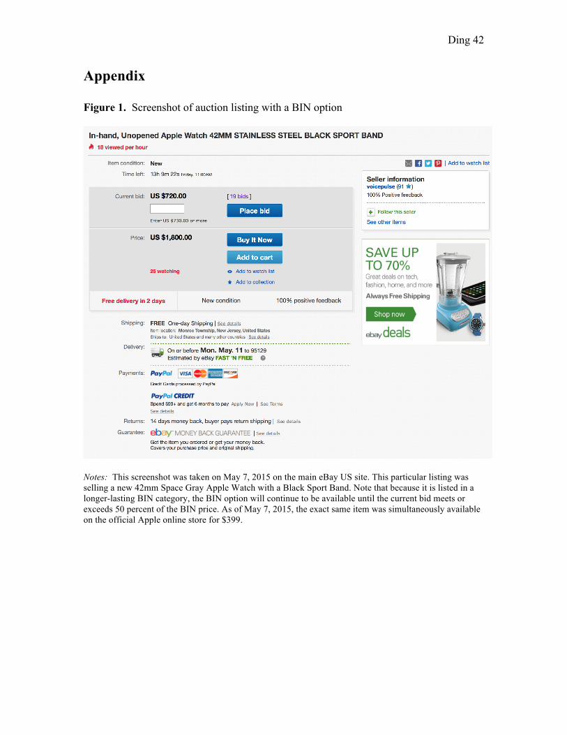
Ding 42
Appendix
Figure 1. Screenshot of auction listing with a BIN option
Notes: This screenshot was taken on May 7, 2015 on the main eBay US site. This particular listing was selling a new 42mm Space Gray Apple Watch with a Black Sport Band. Note that because it is listed in a longer-lasting BIN category, the BIN option will continue to be available until the current bid meets or exceeds 50 percent of the BIN price. As of May 7, 2015, the exact same item was simultaneously available on the official Apple online store for $399.
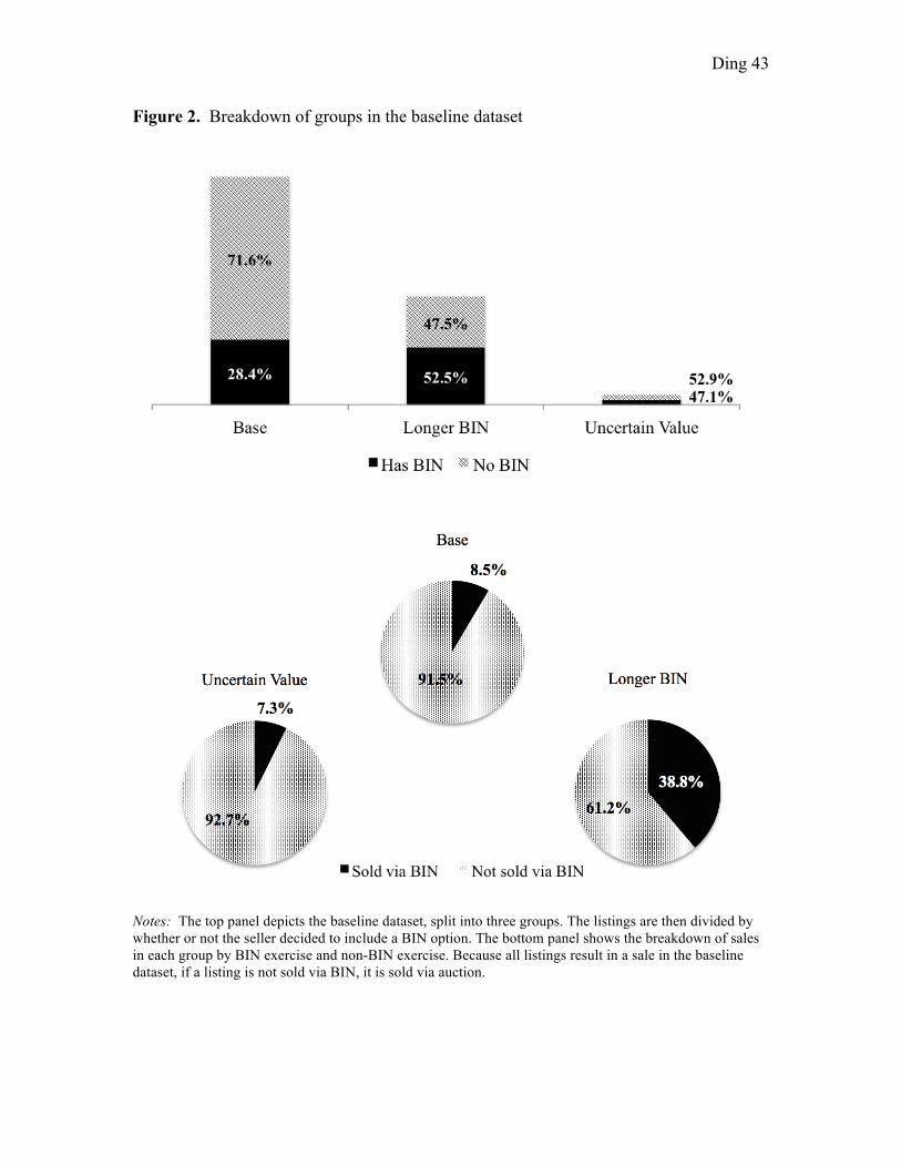
Ding 43
Figure 2. Breakdown of groups in the baseline dataset
Notes: The top panel depicts the baseline dataset, split into three groups. The listings are then divided by whether or not the seller decided to include a BIN option. The bottom panel shows the breakdown of sales in each group by BIN exercise and non-BIN exercise. Because all listings result in a sale in the baseline dataset, if a listing is not sold via BIN, it is sold via auction.

Ding 44
Figure 3. Probability of BIN sale and overpayment by BIN quartile
Notes: This figure shows the effect of the BIN price on the probability of a BIN sale in the solid black line. The probability of overpaying, defined as paying more than the average fixed price, is shown in the broken line. The probability of overpaying, excluding BIN sales, is plotted by the dotted line. The four ranges on the bottom correspond to the four quartiles of normalized BIN prices. Figure 4. Screenshot of auction sale
Notes: This screenshot was taken on May 8, 2015. The listing depicted is the same as the listing shown in Figure 1.
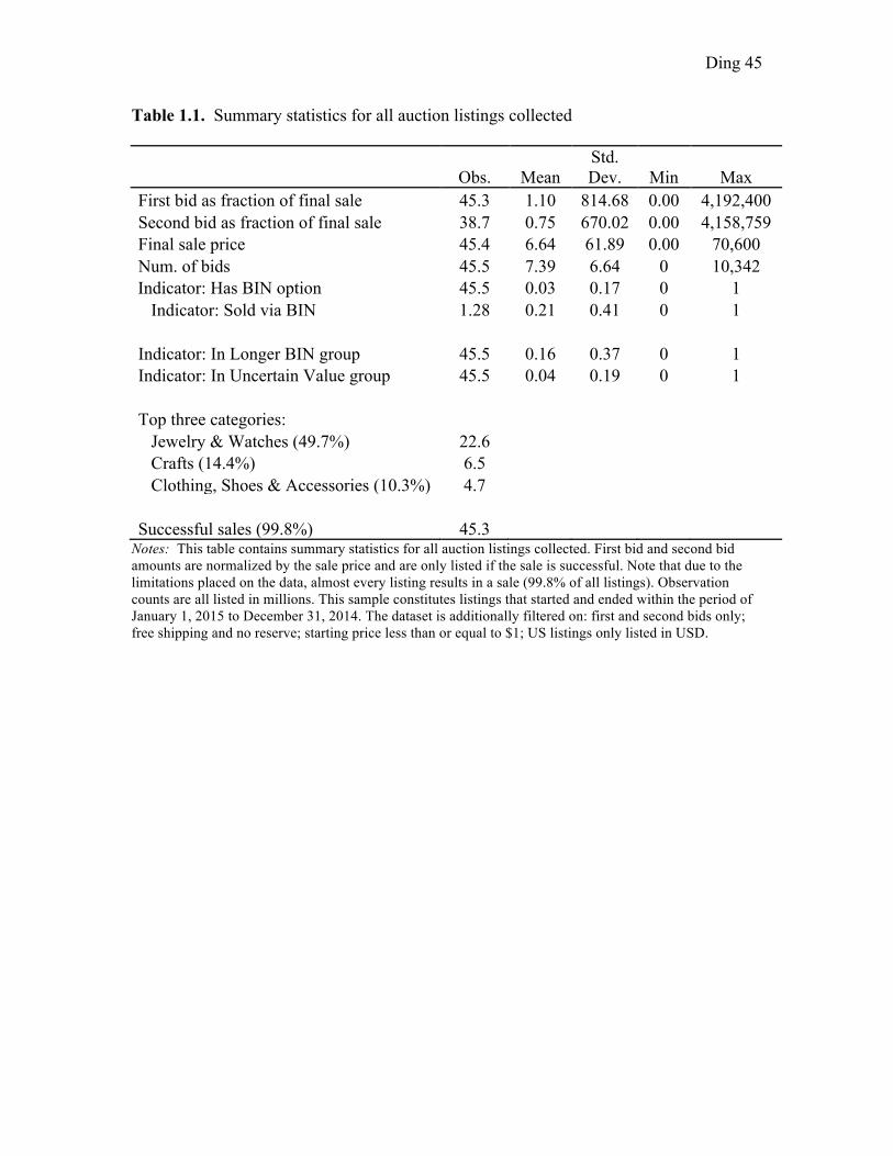
Ding 45
Table 1.1. Summary statistics for all auction listings collected
Obs. Mean
Std. Dev. Min Max
First bid as fraction of final sale 45.3 1.10 814.68 0.00 4,192,400 Second bid as fraction of final sale 38.7 0.75 670.02 0.00 4,158,759 Final sale price 45.4 6.64 61.89 0.00 70,600 Num. of bids 45.5 7.39 6.64 0 10,342 Indicator: Has BIN option 45.5 0.03 0.17 0 1
Indicator: Sold via BIN 1.28 0.21 0.41 0 1
Indicator: In Longer BIN group 45.5 0.16 0.37 0 1 Indicator: In Uncertain Value group 45.5 0.04 0.19 0 1
Top three categories: Jewelry & Watches (49.7%) 22.6
Crafts (14.4%) 6.5 Clothing, Shoes & Accessories (10.3%) 4.7
Successful sales (99.8%) 45.3 Notes: This table contains summary statistics for all auction listings collected. First bid and second bid
amounts are normalized by the sale price and are only listed if the sale is successful. Note that due to the limitations placed on the data, almost every listing results in a sale (99.8% of all listings). Observation counts are all listed in millions. This sample constitutes listings that started and ended within the period of January 1, 2015 to December 31, 2014. The dataset is additionally filtered on: first and second bids only; free shipping and no reserve; starting price less than or equal to $1; US listings only listed in USD.
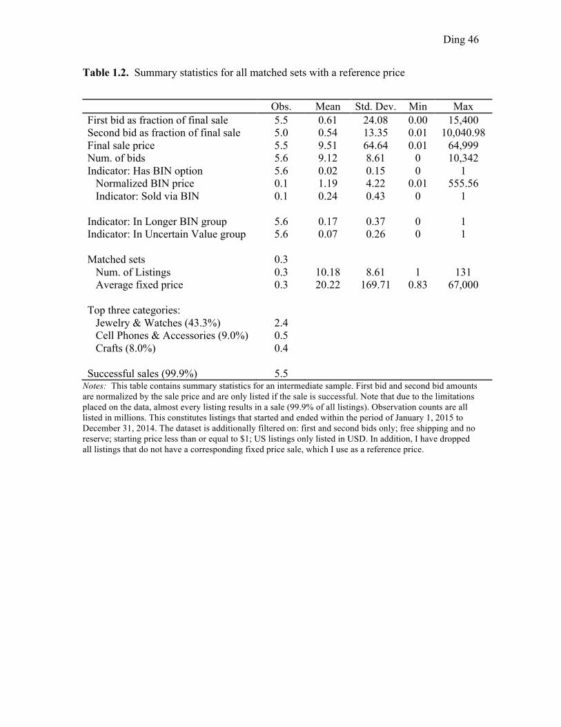
Ding 46
Table 1.2. Summary statistics for all matched sets with a reference price
Notes: This table contains summary statistics for an intermediate sample. First bid and second bid amounts are normalized by the sale price and are only listed if the sale is successful. Note that due to the limitations placed on the data, almost every listing results in a sale (99.9% of all listings). Observation counts are all listed in millions. This constitutes listings that started and ended within the period of January 1, 2015 to December 31, 2014. The dataset is additionally filtered on: first and second bids only; free shipping and no reserve; starting price less than or equal to $1; US listings only listed in USD. In addition, I have dropped all listings that do not have a corresponding fixed price sale, which I use as a reference price.
Obs. Mean Std. Dev. Min Max First bid as fraction of final sale 5.5 0.61 24.08 0.00 15,400 Second bid as fraction of final sale 5.0 0.54 13.35 0.01 10,040.98 Final sale price 5.5 9.51 64.64 0.01 64,999 Num. of bids 5.6 9.12 8.61 0 10,342 Indicator: Has BIN option 5.6 0.02 0.15 0 1
Normalized BIN price 0.1 1.19 4.22 0.01 555.56 Indicator: Sold via BIN 0.1 0.24 0.43 0 1
Indicator: In Longer BIN group 5.6 0.17 0.37 0 1 Indicator: In Uncertain Value group 5.6 0.07 0.26 0 1 Matched sets 0.3
Num. of Listings 0.3 10.18 8.61 1 131 Average fixed price 0.3 20.22 169.71 0.83 67,000
Top three categories:
Jewelry & Watches (43.3%) 2.4 Cell Phones & Accessories (9.0%) 0.5 Crafts (8.0%) 0.4
Successful sales (99.9%) 5.5
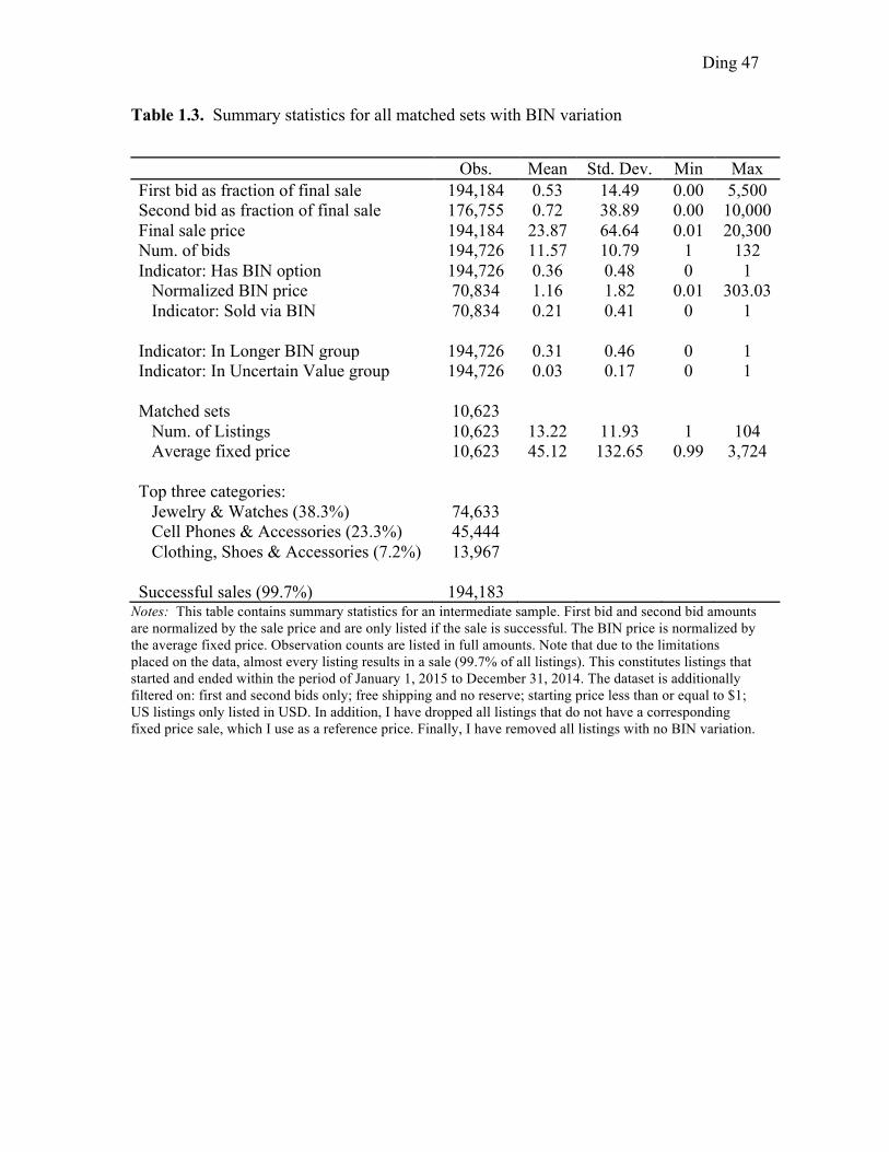
Ding 47
Table 1.3. Summary statistics for all matched sets with BIN variation
Notes: This table contains summary statistics for an intermediate sample. First bid and second bid amounts are normalized by the sale price and are only listed if the sale is successful. The BIN price is normalized by the average fixed price. Observation counts are listed in full amounts. Note that due to the limitations placed on the data, almost every listing results in a sale (99.7% of all listings). This constitutes listings that started and ended within the period of January 1, 2015 to December 31, 2014. The dataset is additionally filtered on: first and second bids only; free shipping and no reserve; starting price less than or equal to $1; US listings only listed in USD. In addition, I have dropped all listings that do not have a corresponding fixed price sale, which I use as a reference price. Finally, I have removed all listings with no BIN variation.
Obs. Mean Std. Dev. Min Max First bid as fraction of final sale 194,184 0.53 14.49 0.00 5,500 Second bid as fraction of final sale 176,755 0.72 38.89 0.00 10,000 Final sale price 194,184 23.87 64.64 0.01 20,300 Num. of bids 194,726 11.57 10.79 1 132 Indicator: Has BIN option 194,726 0.36 0.48 0 1
Normalized BIN price 70,834 1.16 1.82 0.01 303.03 Indicator: Sold via BIN 70,834 0.21 0.41 0 1
Indicator: In Longer BIN group 194,726 0.31 0.46 0 1 Indicator: In Uncertain Value group 194,726 0.03 0.17 0 1 Matched sets 10,623
Num. of Listings 10,623 13.22 11.93 1 104 Average fixed price 10,623 45.12 132.65 0.99 3,724
Top three categories:
Jewelry & Watches (38.3%) 74,633 Cell Phones & Accessories (23.3%) 45,444 Clothing, Shoes & Accessories (7.2%) 13,967
Successful sales (99.7%) 194,183
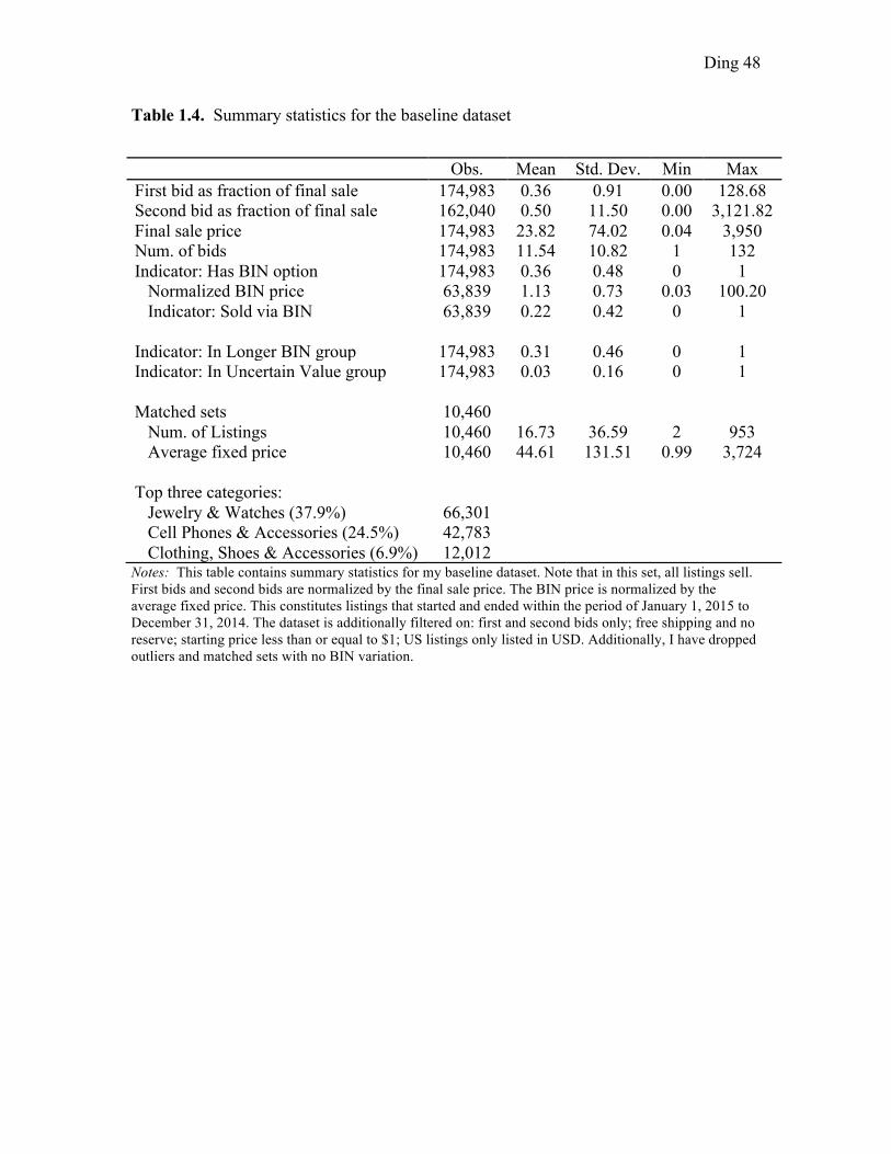
Ding 48
Table 1.4. Summary statistics for the baseline dataset
Notes: This table contains summary statistics for my baseline dataset. Note that in this set, all listings sell. First bids and second bids are normalized by the final sale price. The BIN price is normalized by the average fixed price. This constitutes listings that started and ended within the period of January 1, 2015 to December 31, 2014. The dataset is additionally filtered on: first and second bids only; free shipping and no reserve; starting price less than or equal to $1; US listings only listed in USD. Additionally, I have dropped outliers and matched sets with no BIN variation.
Obs. Mean Std. Dev. Min Max First bid as fraction of final sale 174,983 0.36 0.91 0.00 128.68 Second bid as fraction of final sale 162,040 0.50 11.50 0.00 3,121.82 Final sale price 174,983 23.82 74.02 0.04 3,950 Num. of bids 174,983 11.54 10.82 1 132 Indicator: Has BIN option 174,983 0.36 0.48 0 1
Normalized BIN price 63,839 1.13 0.73 0.03 100.20 Indicator: Sold via BIN 63,839 0.22 0.42 0 1
Indicator: In Longer BIN group 174,983 0.31 0.46 0 1 Indicator: In Uncertain Value group 174,983 0.03 0.16 0 1 Matched sets 10,460
Num. of Listings 10,460 16.73 36.59 2 953 Average fixed price 10,460 44.61 131.51 0.99 3,724
Top three categories:
Jewelry & Watches (37.9%) 66,301 Cell Phones & Accessories (24.5%) 42,783 Clothing, Shoes & Accessories (6.9%) 12,012
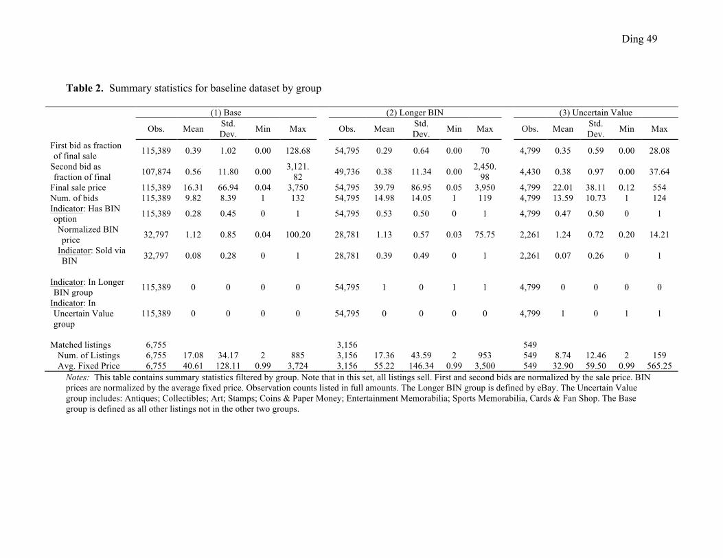
Ding 49
Table 2. Summary statistics for baseline dataset by group
(1) Base (2) Longer BIN (3) Uncertain Value
Obs. Mean Std. Dev. Min Max Obs. Mean Std.
Dev. Min Max Obs. Mean Std. Dev. Min Max
First bid as fraction of final sale 115,389 0.39 1.02 0.00 128.68 54,795 0.29 0.64 0.00 70 4,799 0.35 0.59 0.00 28.08
Second bid as fraction of final 107,874 0.56 11.80 0.00 3,121.
82 49,736 0.38 11.34 0.00 2,450.
98 4,430 0.38 0.97 0.00 37.64
Final sale price 115,389 16.31 66.94 0.04 3,750 54,795 39.79 86.95 0.05 3,950 4,799 22.01 38.11 0.12 554 Num. of bids 115,389 9.82 8.39 1 132 54,795 14.98 14.05 1 119 4,799 13.59 10.73 1 124 Indicator: Has BIN option 115,389 0.28 0.45 0 1 54,795 0.53 0.50 0 1 4,799 0.47 0.50 0 1
Normalized BIN price 32,797 1.12 0.85 0.04 100.20 28,781 1.13 0.57 0.03 75.75 2,261 1.24 0.72 0.20 14.21
Indicator: Sold via BIN 32,797 0.08 0.28 0 1 28,781 0.39 0.49 0 1 2,261 0.07 0.26 0 1
Indicator: In Longer BIN group 115,389 0 0 0 0 54,795 1 0 1 1 4,799 0 0 0 0
Indicator: In Uncertain Value group
115,389 0 0 0 0
54,795 0 0 0 0
4,799 1 0 1 1
Matched listings 6,755 3,156 549
Num. of Listings 6,755 17.08 34.17 2 885 3,156 17.36 43.59 2 953 549 8.74 12.46 2 159 Avg. Fixed Price 6,755 40.61 128.11 0.99 3,724 3,156 55.22 146.34 0.99 3,500 549 32.90 59.50 0.99 565.25
Notes: This table contains summary statistics filtered by group. Note that in this set, all listings sell. First and second bids are normalized by the sale price. BIN prices are normalized by the average fixed price. Observation counts listed in full amounts. The Longer BIN group is defined by eBay. The Uncertain Value group includes: Antiques; Collectibles; Art; Stamps; Coins & Paper Money; Entertainment Memorabilia; Sports Memorabilia, Cards & Fan Shop. The Base group is defined as all other listings not in the other two groups.
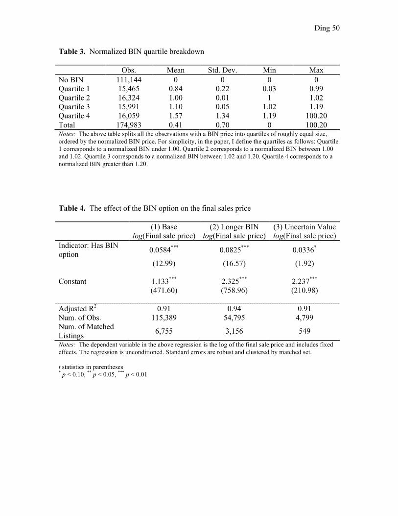
Ding 50
Table 3. Normalized BIN quartile breakdown
Obs. Mean Std. Dev. Min Max No BIN 111,144 0 0 0 0 Quartile 1 15,465 0.84 0.22 0.03 0.99 Quartile 2 16,324 1.00 0.01 1 1.02 Quartile 3 15,991 1.10 0.05 1.02 1.19 Quartile 4 16,059 1.57 1.34 1.19 100.20 Total 174,983 0.41 0.70 0 100.20 Notes: The above table splits all the observations with a BIN price into quartiles of roughly equal size, ordered by the normalized BIN price. For simplicity, in the paper, I define the quartiles as follows: Quartile 1 corresponds to a normalized BIN under 1.00. Quartile 2 corresponds to a normalized BIN between 1.00 and 1.02. Quartile 3 corresponds to a normalized BIN between 1.02 and 1.20. Quartile 4 corresponds to a normalized BIN greater than 1.20.
Table 4. The effect of the BIN option on the final sales price
(1) Base (2) Longer BIN (3) Uncertain Value log(Final sale price) log(Final sale price) log(Final sale price) Indicator: Has BIN option 0.0584*** 0.0825*** 0.0336*
(12.99) (16.57) (1.92) Constant 1.133*** 2.325*** 2.237*** (471.60) (758.96) (210.98) Adjusted R2 0.91 0.94 0.91 Num. of Obs. 115,389 54,795 4,799 Num. of Matched Listings 6,755 3,156 549
Notes: The dependent variable in the above regression is the log of the final sale price and includes fixed effects. The regression is unconditioned. Standard errors are robust and clustered by matched set. t statistics in parentheses * p < 0.10, ** p < 0.05, *** p < 0.01
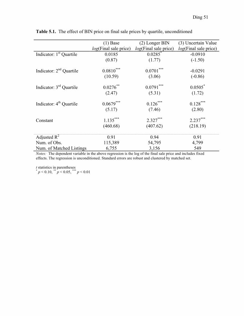
Ding 51
Table 5.1. The effect of BIN price on final sale prices by quartile, unconditioned (1) Base (2) Longer BIN (3) Uncertain Value log(Final sale price) log(Final sale price) log(Final sale price) Indicator: 1st Quartile 0.0185 0.0285* -0.0910 (0.87) (1.77) (-1.50) Indicator: 2nd Quartile 0.0810*** 0.0701*** -0.0291 (10.59) (3.06) (-0.86) Indicator: 3rd Quartile 0.0276** 0.0791*** 0.0505* (2.47) (5.31) (1.72) Indicator: 4th Quartile 0.0679*** 0.126*** 0.128*** (5.17) (7.46) (2.80) Constant 1.135*** 2.327*** 2.237*** (460.68) (407.62) (218.19) Adjusted R2 0.91 0.94 0.91 Num. of Obs. 115,389 54,795 4,799 Num. of Matched Listings 6,755 3,156 549 Notes: The dependent variable in the above regression is the log of the final sale price and includes fixed effects. The regression is unconditioned. Standard errors are robust and clustered by matched set. t statistics in parentheses * p < 0.10, ** p < 0.05, *** p < 0.01

Ding 52
Table 5.2. The effect of BIN price on final sale prices by quartile, conditioned
(1) Base (2) Longer BIN (3) Uncertain Value
log(Final sale price)
log(Final sale price)
log(Final sale price)
Indicator: 1st Quartile -0.0279*** -0.0829*** -0.119*** (-3.28) (-8.26) (-4.02) Indicator: 2nd Quartile 0.0105* -0.0491*** -0.0518 (1.71) (-4.42) (-1.60) Indicator: 3rd Quartile -0.00950 -0.00720 0.0340 (-1.03) (-0.90) (1.26) Indicator: 4th Quartile 0.0366*** 0.0311*** 0.0974*** (3.67) (3.98) (4.12) Constant 1.136*** 2.463*** 2.265*** (595.75) (883.10) (230.12) Adjusted R2 0.91 0.95 0.91 Num. of Obs. 112,602 43,622 4,634 Num. of Matched Listings 6,718 3,066 545 Notes: The dependent variable in the above regression is the log of the final sale price and includes fixed effects. The regression is conditioned on listings that do not result in a BIN sale. This is to control for the revenue effects of BIN exercise and to isolate the revenue effects of BIN existence. Standard errors are robust and clustered by matched set. t statistics in parentheses * p < 0.10, ** p < 0.05, *** p < 0.01 !
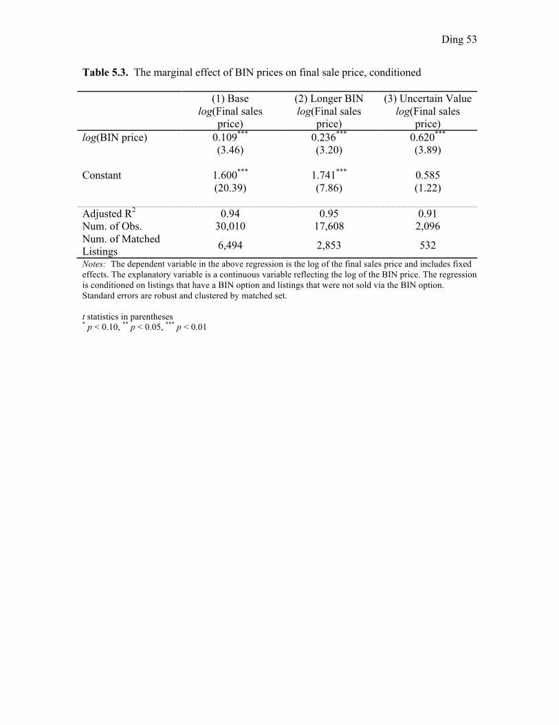
Ding 53
Table 5.3. The marginal effect of BIN prices on final sale price, conditioned (1) Base (2) Longer BIN (3) Uncertain Value
log(Final sales price)
log(Final sales price)
log(Final sales price)
log(BIN price) 0.109*** 0.236*** 0.620*** (3.46) (3.20) (3.89) Constant 1.600*** 1.741*** 0.585 (20.39) (7.86) (1.22) Adjusted R2 0.94 0.95 0.91 Num. of Obs. 30,010 17,608 2,096 Num. of Matched Listings 6,494 2,853 532 Notes: The dependent variable in the above regression is the log of the final sales price and includes fixed effects. The explanatory variable is a continuous variable reflecting the log of the BIN price. The regression is conditioned on listings that have a BIN option and listings that were not sold via the BIN option. Standard errors are robust and clustered by matched set. t statistics in parentheses * p < 0.10, ** p < 0.05, *** p < 0.01 !!!!!!!!!!!!!!!!!!!
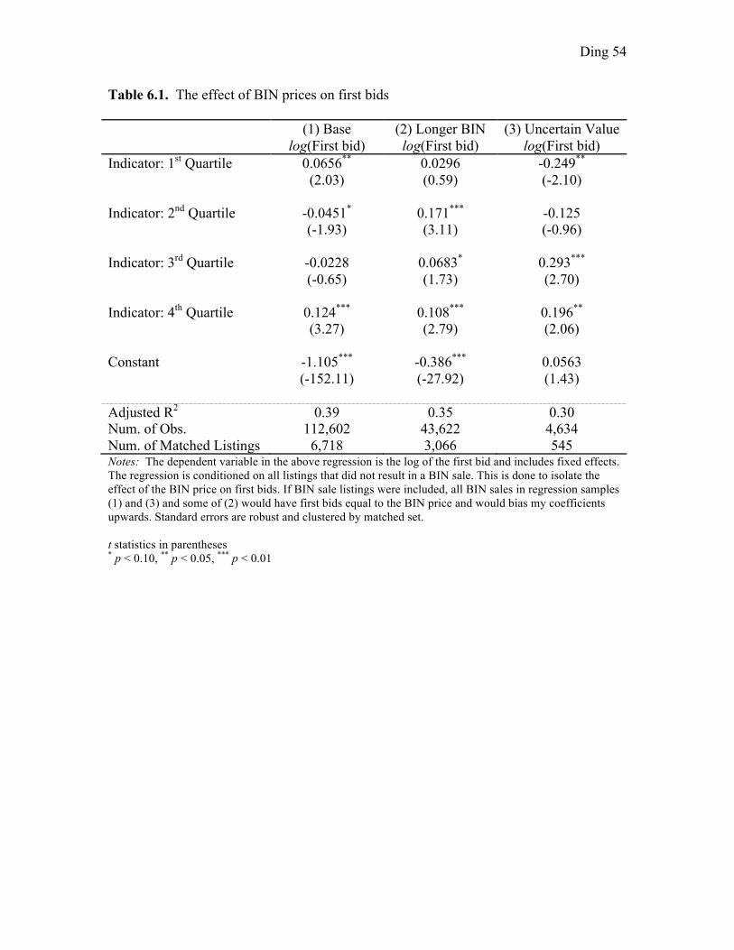
Ding 54
Table 6.1. The effect of BIN prices on first bids (1) Base (2) Longer BIN (3) Uncertain Value log(First bid) log(First bid) log(First bid) Indicator: 1st Quartile 0.0656** 0.0296 -0.249** (2.03) (0.59) (-2.10) Indicator: 2nd Quartile -0.0451* 0.171*** -0.125 (-1.93) (3.11) (-0.96) Indicator: 3rd Quartile -0.0228 0.0683* 0.293*** (-0.65) (1.73) (2.70) Indicator: 4th Quartile 0.124*** 0.108*** 0.196** (3.27) (2.79) (2.06) Constant -1.105*** -0.386*** 0.0563 (-152.11) (-27.92) (1.43) Adjusted R2 0.39 0.35 0.30 Num. of Obs. 112,602 43,622 4,634 Num. of Matched Listings 6,718 3,066 545 Notes: The dependent variable in the above regression is the log of the first bid and includes fixed effects. The regression is conditioned on all listings that did not result in a BIN sale. This is done to isolate the effect of the BIN price on first bids. If BIN sale listings were included, all BIN sales in regression samples (1) and (3) and some of (2) would have first bids equal to the BIN price and would bias my coefficients upwards. Standard errors are robust and clustered by matched set. t statistics in parentheses * p < 0.10, ** p < 0.05, *** p < 0.01
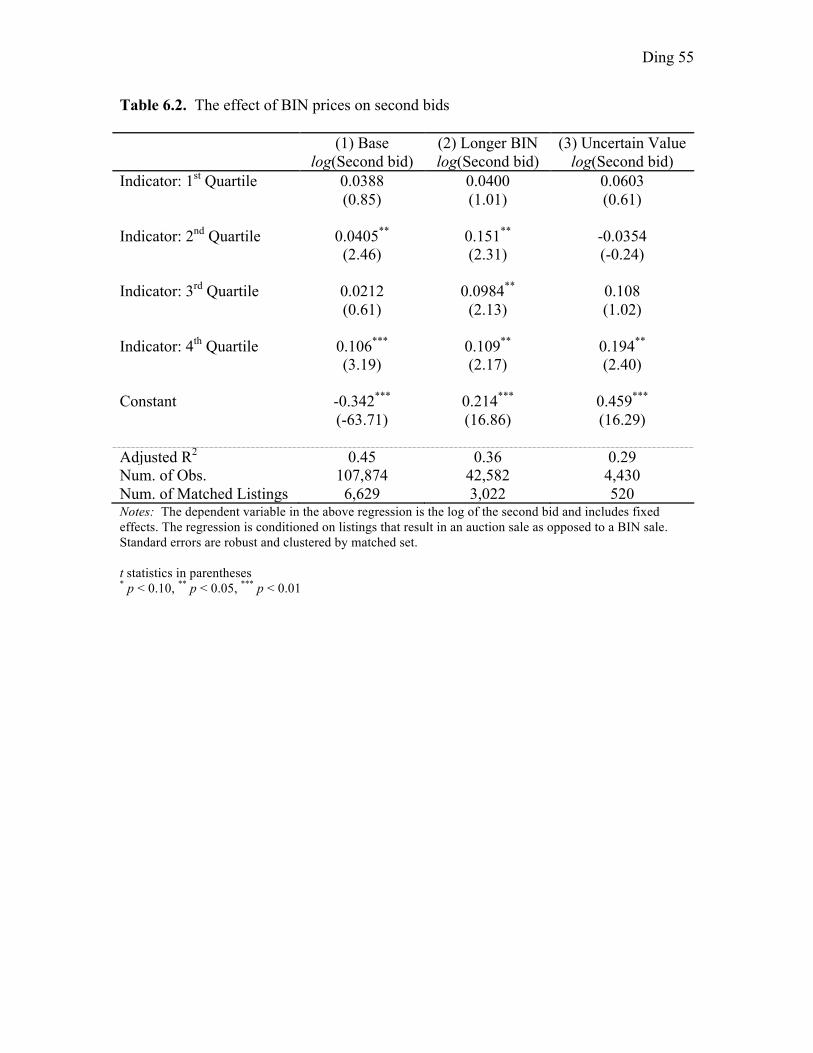
Ding 55
Table 6.2. The effect of BIN prices on second bids (1) Base (2) Longer BIN (3) Uncertain Value log(Second bid) log(Second bid) log(Second bid) Indicator: 1st Quartile 0.0388 0.0400 0.0603 (0.85) (1.01) (0.61) Indicator: 2nd Quartile 0.0405** 0.151** -0.0354 (2.46) (2.31) (-0.24) Indicator: 3rd Quartile 0.0212 0.0984** 0.108 (0.61) (2.13) (1.02) Indicator: 4th Quartile 0.106*** 0.109** 0.194** (3.19) (2.17) (2.40) Constant -0.342*** 0.214*** 0.459*** (-63.71) (16.86) (16.29) Adjusted R2 0.45 0.36 0.29 Num. of Obs. 107,874 42,582 4,430 Num. of Matched Listings 6,629 3,022 520 Notes: The dependent variable in the above regression is the log of the second bid and includes fixed effects. The regression is conditioned on listings that result in an auction sale as opposed to a BIN sale. Standard errors are robust and clustered by matched set. t statistics in parentheses * p < 0.10, ** p < 0.05, *** p < 0.01 !

Ding 56
Table 7. The effect of BIN prices on the number of bids
(1) Base (2) Longer BIN (3) Uncertain Value log(Bid count) log(Bid count) log(Bid count) Indicator: 1st Quartile -0.00859* -0.0447*** 0.000117 (-1.66) (-6.96) (0.01) Indicator: 2nd Quartile 0.0320*** -0.0681*** 0.00496 (7.20) (-8.72) (0.25) Indicator: 3rd Quartile 0.0136** 0.000656 -0.0332* (2.56) (0.14) (-1.83) Indicator: 4th Quartile 0.0150** -0.0173*** -0.00935 (2.44) (-3.51) (-0.53) Num. of Obs. 112,406 43,368 4,609 Num. of Matched Listings 6,718 3,066 545 Notes: The dependent variable in the above regression is the log of the expected count of bids conditional on the BIN quartile and includes fixed effects. The regression is conditioned on all listings that did not result in a BIN sale. This is done in order to control for premature curtailment of the bid count due to a BIN sale. The bid count in this case refers to the total number of bids placed and not the total number of unique bids. Standard errors are robust and clustered by matched set. t statistics in parentheses * p < 0.10, ** p < 0.05, *** p < 0.01
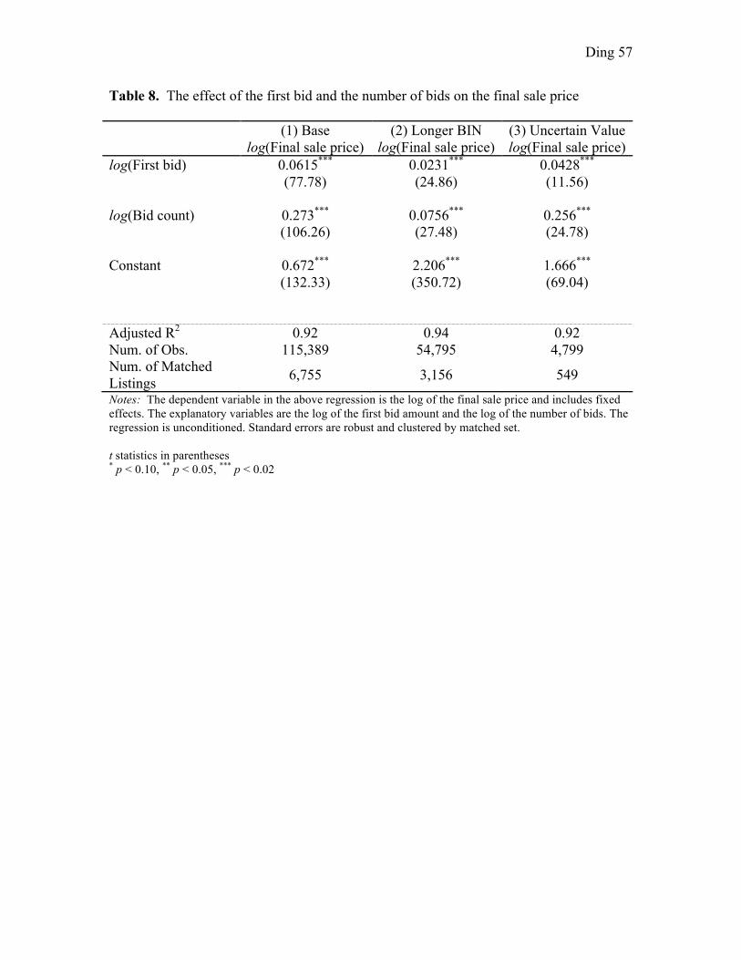
Ding 57
Table 8. The effect of the first bid and the number of bids on the final sale price
(1) Base (2) Longer BIN (3) Uncertain Value log(Final sale price) log(Final sale price) log(Final sale price) log(First bid) 0.0615*** 0.0231*** 0.0428*** (77.78) (24.86) (11.56) log(Bid count) 0.273*** 0.0756*** 0.256*** (106.26) (27.48) (24.78) Constant 0.672*** 2.206*** 1.666*** (132.33) (350.72) (69.04) Adjusted R2 0.92 0.94 0.92 Num. of Obs. 115,389 54,795 4,799 Num. of Matched Listings 6,755 3,156 549 Notes: The dependent variable in the above regression is the log of the final sale price and includes fixed effects. The explanatory variables are the log of the first bid amount and the log of the number of bids. The regression is unconditioned. Standard errors are robust and clustered by matched set. t statistics in parentheses * p < 0.10, ** p < 0.05, *** p < 0.02 !