poverty effects of higher food prices

Policy ReseaRch WoRking PaPeR 4887

Poverty Effects of Higher Food Prices

A Global Perspective

Rafael E. De Hoyos Denis Medvedev

The World BankDevelopment EconomicsDevelopment Prospects GroupMarch 2009

WPS4887P

ublic

Dis

clos

ure

Aut

horiz

edP

ublic

Dis

clos

ure

Aut

horiz

edP

ublic

Dis

clos

ure

Aut

horiz

edP

ublic

Dis

clos

ure

Aut

horiz

ed

Produced by the Research Support Team

Abstract

The Policy Research Working Paper Series disseminates the findings of work in progress to encourage the exchange of ideas about development issues. An objective of the series is to get the findings out quickly, even if the presentations are less than fully polished. The papers carry the names of the authors and should be cited accordingly. The findings, interpretations, and conclusions expressed in this paper are entirely those of the authors. They do not necessarily represent the views of the International Bank for Reconstruction and Development/World Bank and its affiliated organizations, or those of the Executive Directors of the World Bank or the governments they represent.

Policy ReseaRch WoRking PaPeR 4887

The spike in food prices between 2005 and the first half of 2008 has highlighted the vulnerabilities of poor consumers to higher prices of agricultural goods and generated calls for massive policy action. This paper provides a formal assessment of the direct and indirect impacts of higher prices on global poverty using a representative sample of 63 to 93 percent of the population of the developing world. To assess the direct effects, the paper uses domestic food consumer price data between January 2005 and December 2007—when the relative price of food rose by an average of 5.6 percent —to find that the implied increase in the extreme poverty

This paper—a product of the Development Prospects Group, Development Economics—is part of a larger effort in the department to monitor the poverty and income distribution impacts of global economic trends and policies. Policy Research Working Papers are also posted on the Web at http://econ.worldbank.org. The author may be contacted at [email protected].

headcount at the global level is 1.7 percentage points, with significant regional variation. To take the second-order effects into account, the paper links household survey data with a global general equilibrium model, finding that a 5.5 percent increase in agricultural prices (due to rising demand for first-generation biofuels) could raise global poverty in 2010 by 0.6 percentage points at the extreme poverty line and 0.9 percentage points at the moderate poverty line. Poverty increases at the regional level vary substantially, with nearly all of the increase in extreme poverty occurring in South Asia and Sub-Saharan Africa.

Poverty Effects of Higher Food Prices:

A Global Perspective

Rafael E. De Hoyos and Denis Medvedev

Chief of Advisors to the Under-Secretary of Ministry of Education, Mexico, and Economist, Development Prospects Group, World Bank. The views expressed here are those of the authors and should not be attributed to the World Bank, its Executive Directors, or the countries they represent. For their comments we are grateful to Ataman Aksoy, Maurizio Bussolo, Andrew Burns, Nora Lustig, Will Martin, Hans Timmer, Dominique van der Mensbrugghe, and seminar participants at a conference on food prices and poverty organized at the World Bank. Rebecca Lessem and Li Li provided excellent research assistance. The usual caveat applies. Address for correspondence: J9-144, The World Bank Group, 1818 H Street, NW, Washington, DC 20433; [email protected].

1 Introduction The rapid rise in food prices between 2005 and the first half of 2008 has raised numerous concerns about potential negative welfare impacts of a world with higher food prices, particularly among poor households and those with incomes just above the poverty line.1 At the same time, to date there have been few formal assessments of the likely impacts of higher food prices on global poverty, and none using a large sample of developing countries. This paper aims to bridge the existing knowledge gap by providing a set of estimates of the likely impacts of higher food prices on poverty and income distribution at the global level using a unique set of household survey data. The economic effects of changes in relative prices have been a well-researched subject including contributions by Deaton (1989), Ravallion (1990), and Ravallion and van de Walle (1991) among others. According to this literature, changes in food prices can affect poverty and inequality through consumption and income channels (see Figure 1). On the consumer side, as food prices increase, the monetary cost of achieving a fixed consumption basket increases hence reducing consumer’s welfare. However, for the segment of the population whose income depends --directly or indirectly-- on agricultural markets, i.e. self-employed farmers, wage workers in the agricultural sector, and rural land owners, the rise in food prices represents an increase in their monetary income. For each household, the net welfare effect of an increase in food prices will depend on the combination of a loss in purchasing power (consumption effect) and a gain in monetary income (income effect). Clearly, for those households whose income has no linkages with the agricultural markets, for instance urban dwellers, the net welfare effect of an increase in food prices will be entirely determined by the negative consumption effect. For households whose incomes are closely related to the performance of agricultural markets and for which food consumption represents a small proportion of their total budget, higher food prices would be welfare-improving. Therefore, the first-order, or direct, welfare effects of shifts in food prices will be determined by the household’s net position on food supply or demand. In the medium run, once quantities produced are adjusted to reflect the new set of prices in the economy, wages and/or employment in the agricultural sectors will increase to attract the necessary factors of production to increase output --this is what it is known as the second-order, or indirect, income effect (see Figure 1).2 The approach depicted in Figure 1 was undertaken in a recent study by Ivanic and Martin (2008). Using detailed household-level information, the authors find that the proportion of the population living below the poverty line has increased as a result of higher food prices in eight of the nine countries included in their study. In a related study, Friedman and Levinsohn (2002) identify the urban poor as the most vulnerable group during a period of food inflation. Ravallion (1990) develops and tests a methodology to assess the

1 Between July 2008 and February 2009, international agricultural prices (in nominal terms) have come down by 32 percent, but are still 45 percent above their January 2005 levels. 2 Arguably, there is also a “second-order effect” taking place in the consumption side, that is, given the new set of prices, the consumer can chose a different consumption basket. This effect is ignored in the present analysis based on the high degree of correlation among food prices and the little scope that the poor have for food consumption substitution.

2

poverty effects of changes in food prices taking into account the induced wage responses caused by price changes. The author finds that, even including induced wage responses in the analysis, rural poverty in Bangladesh tends to increase as a result of an increase in the relative price of food staples. A recent study by Aksoy and Isik-Dikmelik (2008) challenges the idea that higher food prices unambiguously deteriorate the income of the poor. Using household survey data from nine low-income countries, the authors find that net food sellers are disproportionately represented among the poor, hence suggesting that an increase in food prices can transfer income from richer to poorer households. As one can see, the country-specific and global net poverty effect of higher food prices remains an empirical question to be addressed.

Figure 1 Relationship between International Food Prices and Household Welfare

The paper is organized in the following way. A conceptual framework linking international food prices with household real incomes is briefly delineated in Section 2. Based on the importance of price transmission for poverty impacts (see top part of Figure 1), Section 3 shows the recent changes in domestic food price indices for developing countries and compares them to the evolution of the international food price index.

3

Sections 4 and 5 describe the methodology and present the estimates of direct and indirect poverty impacts, respectively. Section 4 develops two simulations: the first one, particularly relevant for urban areas where the income effects tend to be small or non-existing, takes into account the consumption effect only, while the second simulation combines income and consumption effects imputing a household-specific share of agricultural income in rural areas. Section 5 adds the second-order impacts of higher food prices on poverty to the analysis by linking the household survey data with a global general equilibrium model in a macro-micro simulation framework. Scenarios in this section link higher food prices to the recent and expected (2004-2010) trends in the production of biofuels and allow the households (at the macro level) to re-optimize their consumption and labor supply choices. Section 6 offers concluding remarks.

2 Food Prices and Poverty: Conceptual Links An increase in international food prices will redistribute resources domestically as long as the pass-through or link between international and domestic food prices is different from zero (Macro Level in Figure 1). Assuming a positive pass-through effect, the increase in international food prices will be followed by an increase in domestic food prices enhancing a redistribution of resources from non-agricultural to the agricultural sector of the economy. According to Bussolo, De Hoyos and Medvedev (2009), almost 45 percent of the population in the world lives in a household where the main income-generating activity of the household head takes place in the agricultural sector. The authors show that a large share of this agriculture-dependent group, close to 32 percent, is poor and that these so-called “agricultural households” contribute disproportionately to global poverty: three of every four poor people belong to this group (see Table 1). So redistributing resources from agricultural to non-agricultural households --as an outcome of higher food prices-- could help reduce global poverty and inequality via higher incomes for farmers. However, household purchasing power will also deteriorate as a result of the increase in prices, making the link between agricultural trade liberalization and global household welfare a complex one. Higher food prices will enhance a redistribution of real income between net food producers and net food consumers of agricultural products, with the welfare of the former improving at the expense of the latter (see Micro Level in Figure 1).3 Finally, factor prices will also change following the change in prices of final products therefore changing the real incomes of households that are not directly involved in agricultural production (see Meso Level in Figure 1).

Table 1: Poverty is higher among agricultural households even if their incomes are less unequal

Gini (%)

Pop Shares

(%)

Average Monthly Income

(US$ of 1993, PPP) 1-Dollar Poverty

Incidence (%) Poverty Share

(%) Agriculture 44.9 44.8 65.4 31.7 75.9 Non-Agri. 62.8 55.2 328.9 8.1 24.0 World 67.0 1 210.8 18.7 1

Source: Bussolo, De Hoyos and Medvedev (2009)

3 A household is defined as a net producer (consumer) of agricultural products when the monetary income it derives from merchandising these products is greater (smaller) than the amount spent on them.

4

Ultimately, the short- to medium-term poverty effects of higher international food prices will be determined by: (1) the degree of pass-through; (2) the incidence and severity of poverty among net food producers versus net food consumers; and (3) the extent to which higher food prices translate into higher income for farmers (in the form of profits and wages). The degree of pass-through will be, in turn, determined by domestic market conditions such as: government intervention in the form of subsidies or price controls, infrastructure and market access, the degree of domestic competition and trade barriers among others. Net food production/consumption patterns are determined by the importance of the agricultural sector as an income source of the poor and the proportion of total household budget allocated to food consumption. Finally, the relationship between higher food prices and farmer incomes is a function of the heterogeneity in domestic price transmission among large versus small farmers, and the ability of rural factor (labor) markets to adjust to changes in prices of final products.

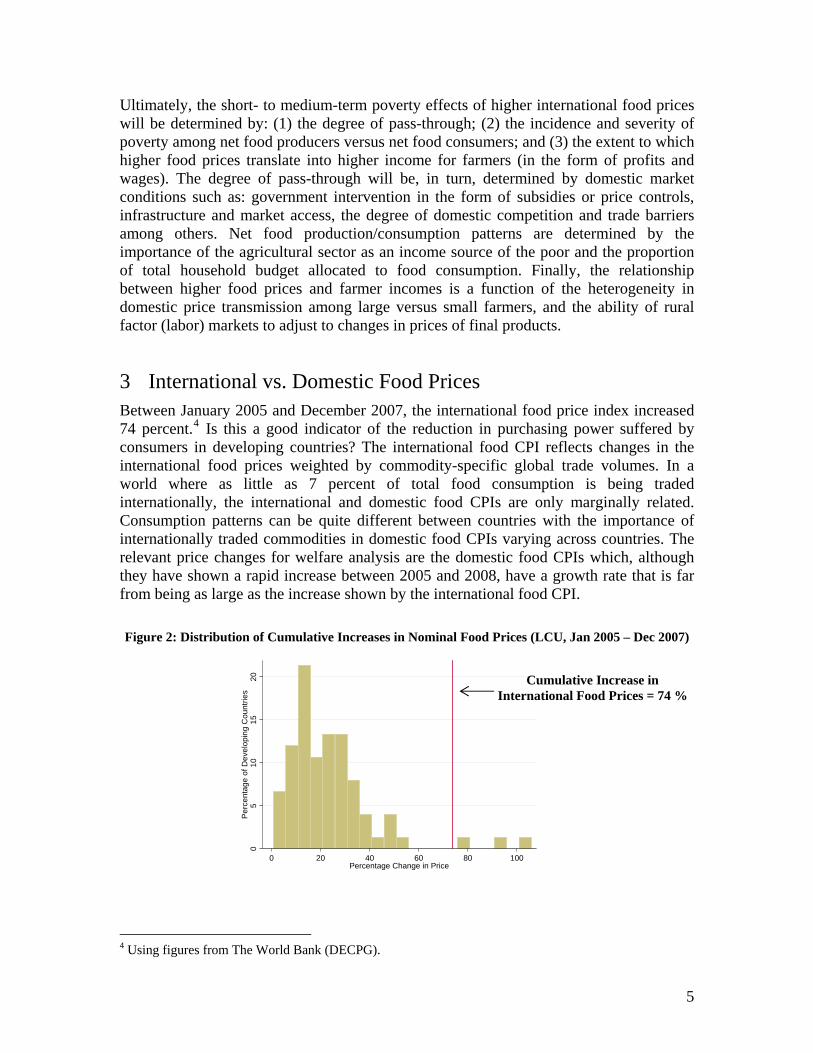
3 International vs. Domestic Food Prices Between January 2005 and December 2007, the international food price index increased 74 percent.4 Is this a good indicator of the reduction in purchasing power suffered by consumers in developing countries? The international food CPI reflects changes in the international food prices weighted by commodity-specific global trade volumes. In a world where as little as 7 percent of total food consumption is being traded internationally, the international and domestic food CPIs are only marginally related. Consumption patterns can be quite different between countries with the importance of internationally traded commodities in domestic food CPIs varying across countries. The relevant price changes for welfare analysis are the domestic food CPIs which, although they have shown a rapid increase between 2005 and 2008, have a growth rate that is far from being as large as the increase shown by the international food CPI.

Figure 2: Distribution of Cumulative Increases in Nominal Food Prices (LCU, Jan 2005 – Dec 2007)

05

10

15

20

Pe

rce

nta

ge

of

De

velo

pin

g C

ou

ntr

ies

0 20 40 60 80 100Percentage Change in Price

Cumulative Increase in International Food Prices = 74 %

4 Using figures from The World Bank (DECPG).

5

Figure 2 shows the domestic increase in food CPI for 76 developing countries between January 2005 and December 2007 and compares it with the increase in the international food CPI.5 In all but three countries, the domestic food price index increased less than the international food prices (74 percent). Differences between the domestic and international food price indices could be explained by differences in the consumption basket with domestic food baskets containing non-traded food items. International and domestic food CPIs can also differ due to: (i) a weak price transmission in internationally traded food commodities (Baffes and Gardner, 2003), (ii) imperfect domestic markets characterized by lack of competition (Levinsohn, 1996) and poor infrastructure, and (iii) government intervention in the form of subsidies and price controls, and other market distortions. The food CPIs in Figure 2 are expressed in local currency units (LCU) and are therefore influenced by local inflation rates. To account for local inflation rates, Figure 3 reports the change in domestic food CPI relative to the change in non-food CPI between January 2005 and December 2007 and compares these indices with the change in international food CPI relative to the manufacturing unit value (MUV) index.6 In 18 of the 76 developing countries included in our sample the non-food price index increased at a faster rate than the change in food prices, in other words, non-food items became relatively more expensive. This is not surprising given the large price increases observed in an important non-food item such as fuels. For the great majority of the developing countries analyzed (58 out of 76) food items became more expensive in terms of non-food items. On average, relative food prices increased 5.6 percent far below the 31 percent increase registered by the international food CPI relative to the MUV.

Figure 3: Distribution of Cumulative Increase in Relative Food Prices (LCU, Jan 2005 – Dec 2007)

05

1015

20P

erce

ntag

e of

Dev

elop

ing

Cou

ntrie

s

-20 0 20 40Percentage Change in Relative Price

Cumulative Increase in International Food Prices = 31 %

As we mentioned before, there are several reasons why domestic and international prices can differ; nevertheless, this section shows that focusing on the international food CPI to

5 The domestic food CPIs are collected by ILO (http://laborsta.ilo.org/) directly from the national statistical offices (or central banks). The international food CPI is constructed by the research department at the World Bank (http://go.worldbank.org/MD63QUPAF1). 6 The MUV index comes from the World Bank (http://go.worldbank.org/VDQ5AA3VP0)

6

http://laborsta.ilo.org/

http://go.worldbank.org/MD63QUPAF1

http://go.worldbank.org/VDQ5AA3VP0

make inferences about the welfare effects of domestic price changes could be misleading. Not only the international food CPI can divert from the average domestic food CPI but also price changes across countries show a high level of heterogeneity. Therefore domestic price indices should be use to infer the ex-post welfare effects of price changes. Changes in domestic nominal prices are more relevant for short-term welfare evaluation since we assume that prices of all non-food items remains constant. On the other hand, relative prices are more appropriate for a medium- to long-run evaluation of the welfare effects of higher food prices. The following section shows the possible poverty effects brought about by the changes in domestic food prices discussed in this section.

4 Direct Poverty Effects of Higher Food Prices

4.1 Methodology

Let us define the monetary income of household “h”, , as the sum of incomes from

profits from agricultural activities, , and incomes deriving from all other sources,

. These monetary income components are assumed to be a function of the vector of

prices in the economy, , hence . The purchasing power of

household “h”, , is defined by the ratio of it money income divided by a household-

specific price index capturing the household’s consumption patters in terms of food and non-food expenditure:

hY

)(P

AhY

hY

NAhY

P )(P NAh

Ah YY

rhY

(1) nf

hf

h

NAh

Ah

h

hrh PP

YY

P

YY

*)1(

)()(

PP

where fP and nfP are food and non-food price indices and h is the proportion of

household’s “h” budget spent on food. Equation (1) captures the dual effect of a price increase depicted in Figure 1, i.e. the possible higher monetary income on the one hand, and the loss in purchasing power on the other. The changes in real incomes brought about

by a change in relative prices of food versus non-food,

pdt

Pnff

Pd

, can be

approximated by the following linear expression: (2) pYpYY hh

Ah

rh

Equation (2) states that, in the short term and for sufficiently small changes in , profits

from farming activities, , will increase in the same proportion as the changes in

relative prices and the loss in purchasing power will be proportional to the amount of the total household budget spent on food,

pA

hY

hhY . Therefore, in the short term, the proportional

change in real income with respect the base period can be written as follows:

7

(3) pY

Yhh

h

rh

)(

where h is the share of total household income that is accrue to profits from farming

activities. Hence, in the short term, higher food prices will benefit net producers of agricultural goods )( hh and hurt net consumers of agricultural products )( hh .

Equations (2) and (3) assume that production and consumption patterns remain constant after the change in prices (Deaton, 1989) and therefore these results should be complemented with a medium- to long-term analysis.

4.2 Simulation Results

The simulations presented here make use of the Global Income Distribution Dynamics (GIDD) dataset that has been recently developed at the World Bank. The GIDD dataset consists of 73 detailed household surveys for low and middle-income countries, 21 of which include information on food expenditure by household.7 Together, this dataset covers 63 percent of the population in the developing world--the major missing country being China. The majority of the surveys (54) use per capita consumption as the welfare indicator, while the remaining surveys--all but one for countries in Latin America--include only per capita income as a measure of household welfare. The welfare measures are expressed in 2005 PPP prices for consistency with the $1.25 and $2.5 a day poverty lines recently developed in Chen and Ravallion (2008).8 All the ex-ante poverty simulations presented in this section capture the ceteris-paribus effects of changes in relative food prices observed between January 2005 and December 2007 (see Figure 3). The results presented here differ from Ivanic and Martin’s (2008) estimates in several ways: (1) the country coverage is substantially different, (2) while Ivanic and Martin’s (2008) focus on the poverty effects of changes in 7 food items, we assess the poverty of changes in prices of the total food basket, (3) Ivanic and Martin’s (2008) use the changes in international prices of their 7 food items as the price shock whereas we use the domestic change in the food CPI relative to the non-food CPI.

4.2.1 Loss in Urban Household Purchasing Power

As it is clear from equation (3), the share of total household budget that is spent on food,

h , is an important element determining the deterioration in purchasing power originated

from an increase in food prices. For some countries, this information is readily available from household surveys, however, in several cases one has to estimate or impute this value. In 21 out of the total 73 countries included in the GIDD’s sample, household-level information on total food expenditure was available. Using the information for these 21

7 See Table 9 in Annex II for a complete country list. A complete description of the dataset is available at http://www.worldbank.org/gidd 8 Most of the household surveys in the GIDD are for years between 2000 and 2005. When the GIDD dataset did not include the newest household survey available from the World Bank’s PovCal, the GIDD’s survey mean income (or consumption) was modified so that the extreme poverty headcount matched the latest information available from PovCal.

8

relatively large countries, a developing countries’ Engel curve was estimated which was then used to impute the values of food shares in all other countries, h

pYh

; the

methodological details if this procedure are explained in De Hoyos and Lessem (2008), which echoes the techniques developed in Cranfield, Preckel, Eales and Hertel (2002). For urban dwellers, where, most likely, the quantities of food produced are close to zero, the welfare effects of higher food prices will be largely determined by the loss in purchasing power. To capture the small income effects in urban areas, we assume that

in equation (2) is zero for all households in this strata, therefore Y . The

results of the simulation focusing on the loss in purchasing power in urban areas can be seen as an instructive way of summarizing the following country-specific information: i) domestic changes in food prices, ii) the initial incidence and severity of poverty in urban areas, iii) the proportion of the total budget spent on food among poor urban households.

AhY h

rh

Table 2 shows the urban poverty impacts of the negative consumption effects brought about by the increase in the relative price of food using a poverty line of $1.25 per day in 2005. Given the large number of results, Table 2 shows regional weighted average poverty effects, however country-specific impacts can be requested from the authors. According to Table 2, the extreme poverty headcount in urban areas increased by 2.86 percentage points as a result of the rise in food prices observed between January 2005 and December 2007. Additionally, the average gap between the poor’s income and the poverty line grew 0.51 percentage points. This deterioration in the poverty indices translates into an additional 68 million individuals below the poverty line and an increase of [20.6] percent in the monetary cost of alleviating total urban poverty under perfect targeting conditions.9 To understand better the relationship between food prices and urban poverty Table 2 presents the elements that determine the increase in urban poverty: (1) the relative change in domestic food prices faced by urban households; (2) the proportion of the total budget that poor urban households allocate to food; and (3) the initial incidence and intensity of poverty among urban dwellers. As it was discussed in Section 2, the magnitude of the food price increase faced by households is, in all regions, significantly lower than the changes registered by the international food price index. The weighted average increase in relative food CPI for urban areas in the developing world is 4.10 percent with food prices increasing at slower rates in Latin America and the Caribbean (LAC) and Eastern Europe and Central Asia (ECA) and quite the opposite in East Asia and the Pacific (EAP) and the Middle East and North Africa (MENA). Notice that, on average, food prices decreased with respect non-food prices in ECA, as it was mention earlier, this could be the result of higher energy prices in this region. LAC and ECA are regions where the expected poverty effects are mild given that poor households in Latin America spend a relatively low proportion of their total budget on food and because the initial poverty rates in these two regions are rather low. On the other hand, poverty indicators in other regions show a considerable

9 Using the change in the poverty deficit as the cost measurement, Dessus, Herrera, and de Hoyos (2008) show that, on average, 90 percent of the additional cost of alleviating urban poverty can be attributable to the reduction of real income of households classified as poor before the price increase.

9

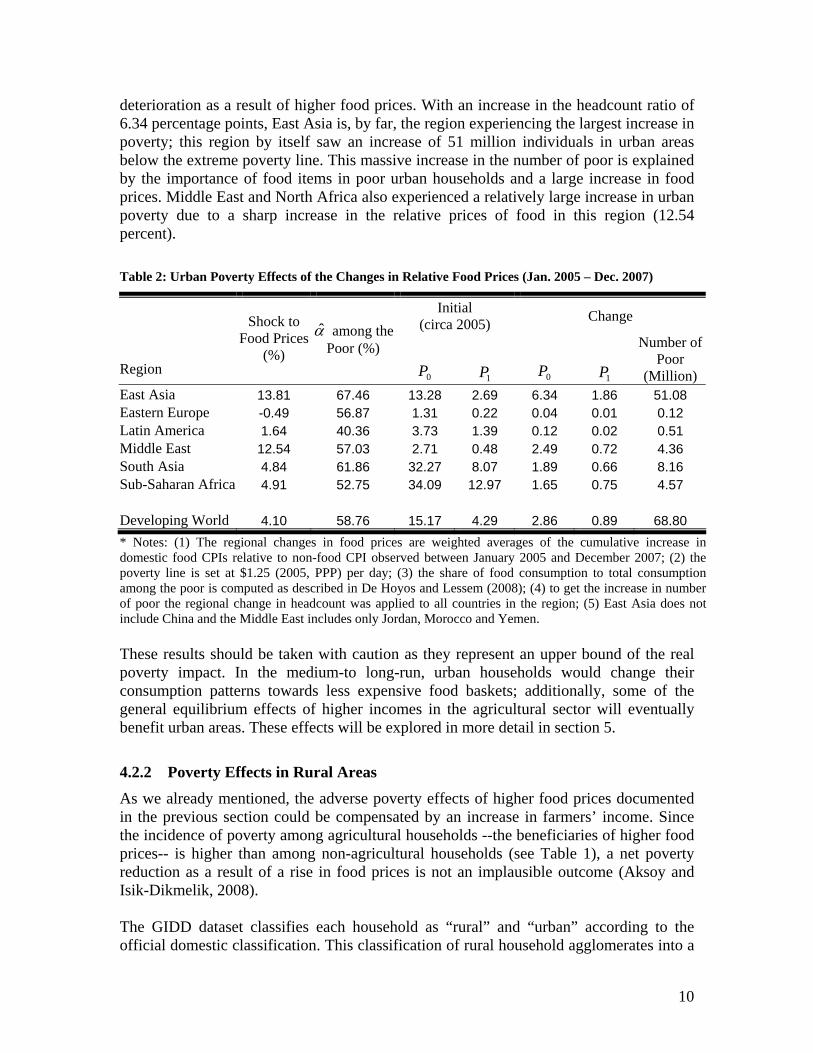
deterioration as a result of higher food prices. With an increase in the headcount ratio of 6.34 percentage points, East Asia is, by far, the region experiencing the largest increase in poverty; this region by itself saw an increase of 51 million individuals in urban areas below the extreme poverty line. This massive increase in the number of poor is explained by the importance of food items in poor urban households and a large increase in food prices. Middle East and North Africa also experienced a relatively large increase in urban poverty due to a sharp increase in the relative prices of food in this region (12.54 percent).

Table 2: Urban Poverty Effects of the Changes in Relative Food Prices (Jan. 2005 – Dec. 2007)

Initial (circa 2005)

Change

Region

Shock to Food Prices

(%)

among the Poor (%)

0P 1P 0P 1P

Number of Poor

(Million) East Asia 13.81 67.46 13.28 2.69 6.34 1.86 51.08 Eastern Europe -0.49 56.87 1.31 0.22 0.04 0.01 0.12 Latin America 1.64 40.36 3.73 1.39 0.12 0.02 0.51 Middle East 12.54 57.03 2.71 0.48 2.49 0.72 4.36 South Asia 4.84 61.86 32.27 8.07 1.89 0.66 8.16 Sub-Saharan Africa 4.91 52.75 34.09 12.97 1.65 0.75 4.57 Developing World 4.10 58.76 15.17 4.29 2.86 0.89 68.80

* Notes: (1) The regional changes in food prices are weighted averages of the cumulative increase in domestic food CPIs relative to non-food CPI observed between January 2005 and December 2007; (2) the poverty line is set at $1.25 (2005, PPP) per day; (3) the share of food consumption to total consumption among the poor is computed as described in De Hoyos and Lessem (2008); (4) to get the increase in number of poor the regional change in headcount was applied to all countries in the region; (5) East Asia does not include China and the Middle East includes only Jordan, Morocco and Yemen. These results should be taken with caution as they represent an upper bound of the real poverty impact. In the medium-to long-run, urban households would change their consumption patterns towards less expensive food baskets; additionally, some of the general equilibrium effects of higher incomes in the agricultural sector will eventually benefit urban areas. These effects will be explored in more detail in section 5.

4.2.2 Poverty Effects in Rural Areas

As we already mentioned, the adverse poverty effects of higher food prices documented in the previous section could be compensated by an increase in farmers’ income. Since the incidence of poverty among agricultural households --the beneficiaries of higher food prices-- is higher than among non-agricultural households (see Table 1), a net poverty reduction as a result of a rise in food prices is not an implausible outcome (Aksoy and Isik-Dikmelik, 2008). The GIDD dataset classifies each household as “rural” and “urban” according to the official domestic classification. This classification of rural household agglomerates into a

10

single group: large land owners, self-sufficient farmers, agricultural wage earners, and households that indeed do not derive income from agricultural activities. Additionally, the GIDD dataset identifies a welfare aggregate (income or consumption) only at the household level. This posses a serious challenge since, as oppose to the information on food shares, h , we do not have information on the level and distribution of the

proportion of total household income that is accrue to agricultural self-employment activities h . Both h and h vary across households but, as oppose to h there is no

economic theory that we can use to estimate a relationship between h and other

observable characteristics like household per capita income. In order to get plausible values of h we rely on the information from the Rural Income

Generating Activities (RIGA) project. RIGA is a FAO-World Bank funded project that uses LSMS household surveys to disentangle the sources of rural income with the purpose of understanding the relationship between the various income generating activities.10 Taking the reported share of self-employed agricultural income at the household level for 19 countries located in 5 of the 6 World Bank developing regions, we estimate a simple polynomial relationship between the share of income that is attributable to self-employment agricultural incomes, h , and per capital household income (or

consumption), , and regional fixed effects: hy

(4) hh

hhhhh

SASLAC

ECAEAPyy

*49.0*44.0

*30.0*38.0*0002.0*54.076.0ˆ 2

692,930N ; 5.02 R

This simple specification is enough to give a rather good fit of the data with an R2 of 0.5. According to the observed data, controlling for income differences, the share of self-employed income in rural areas is highest in Sub-Saharan Africa and much lower in Latin America and South Asia. The results of this simple specification are used to impute the share of self-employed agricultural income in all rural households taking into account their per-capita household income (or consumption) and regional location. Figure 4 shows the difference between the observed and imputed agricultural self-employed income share for each percentile of per capita consumption in rural areas. The share labeled “all countries” shows that the average share in the poorest households in rural areas is close to 80 percent while this falls to 15 percent for households in upper percentiles. Figure 3 also shows the prediction power of the model by comparing the observed shares, h , versus the fitted values, h , for two rather different countries,

Nigeria and Panama. The country-specific fitted values in Figure 3 are based on two separate regressions that excluded Nigeria and Panama, respectively. Overall, the

10 For more details on the LSMS household surveys see http://www.worldbank.org/LSMS/. For a complete description of the RIGA project including publication of the first results see Carletto et. al. (2007) and visit: http://www.fao.org/es/ESA/riga/index_en.htm

11

http://www.worldbank.org/LSMS/

http://www.fao.org/es/ESA/riga/index_en.htm

imputed share was not substantially different from the observed one, with the average absolute difference between observed and imputed shares in Panama and Nigeria being around 7 percentage points. In the short-run, incomes of self-employed farmers will increase in proportion to the increase in prices of their produce. The lack of household-level information on rural income sources, implies that, as a result of higher food prices, all rural households experience an increase in nominal income equal to pYhh . Therefore, as long as hh ˆˆ ,

household “h” will experience a reduction in real income as a result of higher food prices. For the same increase in price, given the higher value of h estimated by specification

(4), rural households in Sub-Saharan Africa experience a higher increase in nominal income compared with rural households in Latin America.

Figure 4: Observed and Imputed Share of Agricultural SE Income

020

4060

8010

0S

elf-

empl

oym

ent A

gric

ultu

ral S

hare

, %

0 20 40 60 80 100Percentiles of Per-Capita Consumption

(1) Using data from RIGA; (2) the percentiles are country-specific

Nigeria

All Countries

Panama

The rural poverty effects of a simulation accounting for the consumption and income effects assuming hh ˆ are presented in Table 3. Despite the fact that we are allowing

for positive income effects in the relatively poorer rural areas, indicators in all regions show deterioration in terms of the incidence and depth of poverty. Notice that, although the initial poverty headcount is much higher in rural areas, the increase in this poverty indicator is smaller than in urban areas capturing the offsetting income effects of higher food prices taking place in rural households. For each region except for Latin America, the change in the rural poverty headcount ratio is smaller than the change taking place in urban areas. At the global level, the headcount ratio in rural areas increases by 2.06 percentage points representing an additional 87.19 million individuals falling below the poverty line. The rural poverty deficit, i.e. the resources needed to alleviate extreme

12

poverty in rural areas, jumps by 6 percent after the change in relative prices--much lower than 21 percent increase taking place in urban areas. Given the importance of self-employed agricultural incomes for rural households in Sub-Saharan Africa, higher food prices are not translated into a significantly higher poverty rate in this region. Despite the relatively mild increase in the incidence of poverty in rural South Asia an extra 19.5 million individuals fall short the extreme poverty line after the price shock. As in urban areas, the deterioration of rural poverty indicators is more acute in East Asia with this region accounting for 62 million out of the total 87 million new poor.

Table 3: Rural Poverty Effects of the Changes in Relative Food Prices (Jan. 2005 – Dec. 2007)


Change

Region


(%)

Food Share Among the Poor (% of

total Y) 0P 1P 0P 1P

Number of Poor


* Notes: (1) The regional changes in food prices are weighted averages of the cumulative increase in domestic food CPIs relative to non-food CPI observed between January 2005 and December 2007; (2) the poverty line is set at $1.25 (2005, PPP) per day; (3) the share of food consumption to total consumption among the poor is computed as described in De Hoyos and Lessem (2008); (4) to get the increase in number of poor the regional change in headcount was applied to all countries in the region; (5) East Asia does not include China and the Middle East includes only Jordan, Morocco and Yemen.

4.2.3 Total Poverty Effects

Overall, the number of individuals living on less than $1.25 a day, 2005 PPP increased by 155 million as a result of the cumulative increase in the relative price of food observed between January 2005 and December 2007 (see Table 4). Notice that this result contrasts with the 105 million reported in Ivanic and Martin (2008). There are several reasons behind this difference: (i) the present paper uses data for 73 developing countries as opposed to 9, (ii) the estimates of Ivanic and Martin (2008) are based on nominal price changes for 7 commodities whereas our study takes the cumulative change in food CPI relative to non-food CPI as the price shock, (iii) the income/consumption household aggregates are expressed in 2005 PPP and the newly developed $1.25 and $2.5 poverty lines are used to measure the initial poverty indices (see Chen and Ravallion, 2008), and (iv) Ivanic and Martin (2008) total poverty estimates are valid for low-income countries covering a total population of 2.3 billion whereas our estimates are for all the developing world covering a population equal to 5.4 billion. Given all these differences, the

13

discrepancy of 50 million between the number of new poor presented in this study and the number of new poor estimated in Ivanic and Martin (2008) is indeed a small one.

Table 4: Total Poverty Effects of the Changes in Relative Food Prices (Jan. 2005 – Dec. 2007)


Change

Region


(%)

Food Share Among the Poor (% of

total Y) 0P

1P 0P 1P

Number of Poor


* Notes: (1) The regional changes in food prices are weighted averages of the cumulative increase in domestic food CPIs relative to non-food CPI observed between January 2005 and December 2007; (2) the poverty line is set at $1.25 (2005, PPP) per day; (3) the share of food consumption to total consumption among the poor is computed as described in De Hoyos and Lessem (2008); (4) to get the increase in number of poor the regional change in headcount was applied to all countries in the region; (5) East Asia does not include China and the Middle East includes only Jordan, Morocco and Yemen. The results presented in Table 4 hide important heterogeneities across countries. Figure 5 shows the changes in poverty headcount and gap for each of the countries in our sample. The changes in food prices have different impacts in different countries with the net poverty effect --in terms of poverty headcount and gap-- being close to zero (less than a fifth of a percentage point) for 60 percent of the countries included in our sample. In around half of the developing countries analyzed, higher food prices raise the headcount ratio by at least 0.2 percentage points; Indonesia, Yemen, Ethiopia, Pakistan, and Bangladesh are the countries with the highest adverse poverty effects with increases in the headcount ratio of more than 3.5 percentage points. By contrast, in 7 developing countries the change in relative prices reduces the incidence of poverty by at least 2 percentage points. In 5 of these 7 countries, the reduction in poverty is attributable to a reduction in relative food prices (Dominican Republic, Sri Lanka, Madagascar, Benin, and Moldova). Nevertheless, in Kenya and Mali the reduction in poverty in rural areas is large enough to compensate for the poverty increase observed in the cities and pull down the national poverty headcount by 0.42 and 0.75 percentage points, respectively.

14

Figure 5: Changes in the Poverty Headcount and Gap due to the Increase in Food Prices

Notes: (1) the poverty line is set at $1.25 (2005, PPP) per day; (2) using data from the GIDD.

5 Incorporating Indirect Poverty Effects of Higher Food Prices Although international agricultural prices have retreated substantially from their peak in July 2008, they remain more than 45 percent above their January 2005 level. While this is clearly not convincing evidence of a reversal in the long-term trend of declining agricultural prices, there are several reasons why the scope for additional declines may be limited: slower progress in development of new technologies, limited take-up of existing advanced techniques due to infrastructure and institutional constraints, sooner- or larger-than-expected damages from climate change, or large and growing additional demand for agricultural output from biofuels. In fact, the latter has played a major role in the 2005-2008 spike in food prices, according to Mitchell (2008) and World Bank (2009, Chapter 2). This section explores the implications of the continued high demand for first-generation biofuels through 2010, satisfied through increased production of corn, sugar cane, and wheat for ethanol, and oil seeds for biodiesel. This is done by linking a recursive-dynamic global computable equilibrium (CGE) model with the GIDD micro-simulation model. The CGE model contrasts a baseline scenario, in which the demand for biofuels (as a share of total demand for a specific crop) remains at 2004 levels, with a biofuels scenario in which demand follows its historical path through 2007 and is projected through 2010 using current mandates and production trends.

5.1 Methodology

The general equilibrium model used in this paper is the World Bank's Environmental Impacts and Sustainability Applied General Equilibrium model (ENVISAGE). The detailed description is available in van der Mensbrugghe (2008), while the next two paragraphs summarize its most relevant features. Production is modeled with a series of nested CES functions that allow for different degrees of substitutability across inputs, which include intermediate inputs, energy, skilled and unskilled labor, different capital

15

vintages, land, and natural resources. The latter are sector-specific, while land has limited transformation across agricultural uses. New capital vintages and skilled labor are freely mobile across sectors, while the mobility of old vintages is limited. Unskilled workers are freely mobile within farm and non-farm activities, but the movement from farm to non-farm employment is limited with a Harris-Todaro migration function. Consumer demand is modeled with a nesting of Cobb-Douglas and constant-differences-in-elasticity (CDE) utility functions. International trade is specified with nested CES and CET functions which allow for limited substitution between domestically produced goods and imports or exports (the Armington assumption). The model contains an integrated climate module which links CO2 emissions to changes in global temperature with feedbacks to agricultural productivity (following the approach of Nordhaus and Boyer, 2000, and Nordhaus, 2007, and calibrated with estimates in Cline, 2007). The current version of the model is based on the GTAP database with a 2004 base year, which has been aggregated to 26 country/regions and 22 sectors (Table 8). The model is solved forward, in recursive fashion, until 2010, with labor force and population growth rates lined up to the UN’s medium variant population forecast. TFP growth in agriculture is set at 2.5 percent per annum with no differentiation across sectors or regions, based on estimates in Martin and Mitra (1999). Labor-augmenting productivity growth in the other sectors is endogenized to achieve the World Bank's forecasted growth of real GDP. The macro closure has government expenditures as a share of GDP fixed at 2004 levels, while a demographically-driven savings function determines the allocation of private expenditures between consumer demand and domestic investment. The manufactured export price index of the high-income countries is the numéraire. The distributional analysis is carried out with the World Bank’s GIDD model, which generalizes the existing CGE-microsimulation methodologies—e.g., Bourguignon, Bussolo, and Pereira da Silva (2008), Chen and Ravallion (2003), and Bussolo, Lay, and van der Mensbrugghe (2006)—at the global level and is described in detail in Bussolo, De Hoyos, and Medvedev (2008a).11 The conceptual framework of the model is depicted in Figure 6. The expected changes in population structure by age (upper left part of Figure 6) are exogenous, meaning that fertility decisions and mortality rates are determined outside the model. The change in shares of the population by education groups incorporates the expected demographic changes (linking arrow from top left box to top right box in Figure 6). Next, new sets of population shares by age and education subgroups are computed and household sampling weights are re-scaled according to the demographic and educational changes above (larger box in the middle of Figure 6). The impact of changes in the demographic structure on labor supply (by skill level) is incorporated into the CGE model, which then provides a set of link variables for the micro-simulation: (a) change in the allocation of workers across sectors in the economy, (b) change in returns to labor by skill and occupation, (c) change in the relative price of food and non-food consumption baskets, and (d) differentiation in per capita income/consumption growth rates across countries. The final distribution is obtained by applying the changes in these link variables to the re-weighted household survey (bottom link in Figure 6). 11 The detailed description of the methodology can also be found at http://www.worldbank.org/gidd

16

The data for the exercise is a combination of the 73 household surveys described earlier in section 4.2 and more aggregate data on income groups (usually vintiles) for 25 high income and 22 developing countries. The final sample covers more than 90 percent of the world’s population (see Table 9 in Annex II for country coverage).

Figure 6: GIDD methodological framework

Population Projection by Age Groups ( Exogenous )

Education Projection(Semi- Exogenous )

Household Survey (new sampling weightsby age and education)

CGE(Growth, New Wages, New Prices, Sectoral Reallocation)

Simulated Distribution

5.2 Simulation Results

In the baseline scenario, prices of agricultural products continue to rise modestly from their 2004 levels, with the total increase reaching nearly 5 percent above the OECD industrial exports price index (MUV) by 2010. This gradual rise in prices is driven partially by lower crop yields due to climate change, partially by a re-orientation of the food consumption basket in developing countries to meats and more processed foods, which raise the demand for feed grains and are thus less ‘efficient’ in meeting caloric intake requirements, and partially by the lack of investment in agriculture due to years of declining prices. However, this rise in agricultural prices is fully offset by a decline in the price of processed food—where large productivity gains are realized in fast-growing developing countries—such that the price of the agriculture and food bundle (at the global level) remains nearly constant throughout the model horizon.

17

When rising demand for biofuels is introduced into the model, agricultural producers dramatically accelerate the output of biofuel crops by shifting resources away from other agricultural activities. This is illustrated in Figure 7, which shows the contribution of each agricultural activity in the model to the total increase in agricultural output. The production increases vary substantially by country and type of grain (Table 5), with the largest gains realized in countries with relatively more abundant land, higher initial demand (e.g., the legislative mandates adopted in the US and the EU), and the existing penetration of biofuel technologies (e.g., Brazil is more competitive in sugar-base ethanol than other producers). At the same time, the supply expansion is limited by the amount of additional land that may be brought under cultivation—which we assume is limited in the six-year horizon of the model—as well as the additional labor that may be attracted to the agricultural sector, which is limited by the large and persistent wage gaps between rural and urban incomes in the developing world.12 Therefore, output of other agricultural goods—such as rice, other crops, and livestock—declines relative to baseline as farmers find it more profitable to focus on biofuels. Given that many biofuels crops use land intensively, the returns to land rise substantially, ranging from above 40 percent in Brazil to just under 4 percent in Japan. The returns to unskilled labor rise substantially less: for developing countries as a whole, unskilled wages increase by 11 percent while land prices go up by 16 percent.

Figure 7 Impact of biofuels on global agricultural production

-1

0

1

2

3

4

5

6

7

2005 2006 2007 2008 2009 2010

Pe

rce

nt

dif

fere

nc

e in

re

al o

utp

ut

rela

tiv

e t

o b

as

elin

e

Rice Wheat Corn Oil seeds

Sugar cane Other crops Livestock Agriculture

Source: Simulations with World Bank’s ENVISAGE model.

12 In other words, although higher prices of agriculture contribute to a faster closing of rural-urban wage gaps in developing countries (relative to the baseline scenario) and reduce the incentive to migrate at the margin, an average agricultural worker still finds it advantageous to move to an urban area where earnings tend to be much higher. This labor market rigidity limits the supply response in developing countries.

18

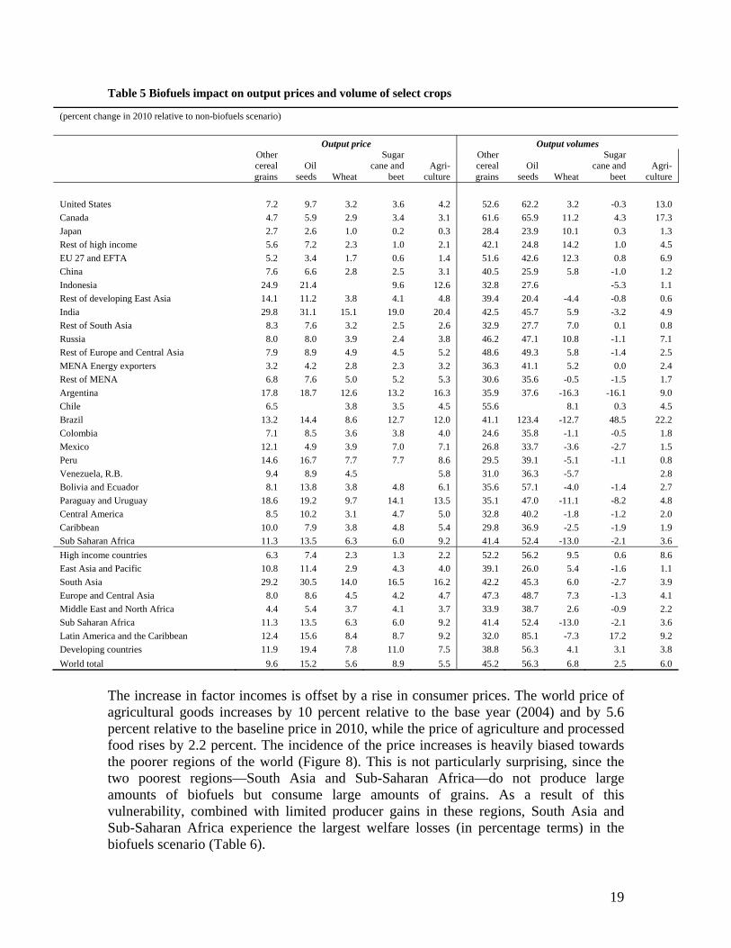
Table 5 Biofuels impact on output prices and volume of select crops

(percent change in 2010 relative to non-biofuels scenario)

Output price Output volumes

Other cereal grains

Oil seeds Wheat

Sugar cane and

beet Agri-

culture

Other cereal grains

Oil seeds Wheat

Sugar cane and

beet Agri-

culture

United States 7.2 9.7 3.2 3.6 4.2 52.6 62.2 3.2 -0.3 13.0

Canada 4.7 5.9 2.9 3.4 3.1 61.6 65.9 11.2 4.3 17.3

Japan 2.7 2.6 1.0 0.2 0.3 28.4 23.9 10.1 0.3 1.3

Rest of high income 5.6 7.2 2.3 1.0 2.1 42.1 24.8 14.2 1.0 4.5

EU 27 and EFTA 5.2 3.4 1.7 0.6 1.4 51.6 42.6 12.3 0.8 6.9

China 7.6 6.6 2.8 2.5 3.1 40.5 25.9 5.8 -1.0 1.2

Indonesia 24.9 21.4 9.6 12.6 32.8 27.6 -5.3 1.1

Rest of developing East Asia 14.1 11.2 3.8 4.1 4.8 39.4 20.4 -4.4 -0.8 0.6

India 29.8 31.1 15.1 19.0 20.4 42.5 45.7 5.9 -3.2 4.9

Rest of South Asia 8.3 7.6 3.2 2.5 2.6 32.9 27.7 7.0 0.1 0.8

Russia 8.0 8.0 3.9 2.4 3.8 46.2 47.1 10.8 -1.1 7.1

Rest of Europe and Central Asia 7.9 8.9 4.9 4.5 5.2 48.6 49.3 5.8 -1.4 2.5

MENA Energy exporters 3.2 4.2 2.8 2.3 3.2 36.3 41.1 5.2 0.0 2.4

Rest of MENA 6.8 7.6 5.0 5.2 5.3 30.6 35.6 -0.5 -1.5 1.7

Argentina 17.8 18.7 12.6 13.2 16.3 35.9 37.6 -16.3 -16.1 9.0

Chile 6.5 3.8 3.5 4.5 55.6 8.1 0.3 4.5

Brazil 13.2 14.4 8.6 12.7 12.0 41.1 123.4 -12.7 48.5 22.2

Colombia 7.1 8.5 3.6 3.8 4.0 24.6 35.8 -1.1 -0.5 1.8

Mexico 12.1 4.9 3.9 7.0 7.1 26.8 33.7 -3.6 -2.7 1.5

Peru 14.6 16.7 7.7 7.7 8.6 29.5 39.1 -5.1 -1.1 0.8

Venezuela, R.B. 9.4 8.9 4.5 5.8 31.0 36.3 -5.7 2.8

Bolivia and Ecuador 8.1 13.8 3.8 4.8 6.1 35.6 57.1 -4.0 -1.4 2.7

Paraguay and Uruguay 18.6 19.2 9.7 14.1 13.5 35.1 47.0 -11.1 -8.2 4.8

Central America 8.5 10.2 3.1 4.7 5.0 32.8 40.2 -1.8 -1.2 2.0

Caribbean 10.0 7.9 3.8 4.8 5.4 29.8 36.9 -2.5 -1.9 1.9

Sub Saharan Africa 11.3 13.5 6.3 6.0 9.2 41.4 52.4 -13.0 -2.1 3.6

High income countries 6.3 7.4 2.3 1.3 2.2 52.2 56.2 9.5 0.6 8.6

East Asia and Pacific 10.8 11.4 2.9 4.3 4.0 39.1 26.0 5.4 -1.6 1.1

South Asia 29.2 30.5 14.0 16.5 16.2 42.2 45.3 6.0 -2.7 3.9

Europe and Central Asia 8.0 8.6 4.5 4.2 4.7 47.3 48.7 7.3 -1.3 4.1

Middle East and North Africa 4.4 5.4 3.7 4.1 3.7 33.9 38.7 2.6 -0.9 2.2

Sub Saharan Africa 11.3 13.5 6.3 6.0 9.2 41.4 52.4 -13.0 -2.1 3.6

Latin America and the Caribbean 12.4 15.6 8.4 8.7 9.2 32.0 85.1 -7.3 17.2 9.2

Developing countries 11.9 19.4 7.8 11.0 7.5 38.8 56.3 4.1 3.1 3.8

World total 9.6 15.2 5.6 8.9 5.5 45.2 56.3 6.8 2.5 6.0

The increase in factor incomes is offset by a rise in consumer prices. The world price of agricultural goods increases by 10 percent relative to the base year (2004) and by 5.6 percent relative to the baseline price in 2010, while the price of agriculture and processed food rises by 2.2 percent. The incidence of the price increases is heavily biased towards the poorer regions of the world (Figure 8). This is not particularly surprising, since the two poorest regions—South Asia and Sub-Saharan Africa—do not produce large amounts of biofuels but consume large amounts of grains. As a result of this vulnerability, combined with limited producer gains in these regions, South Asia and Sub-Saharan Africa experience the largest welfare losses (in percentage terms) in the biofuels scenario (Table 6).

19

Figure 8 Impact of biofuels on consumer prices

0 2 4 6 8 10 12 14 16 18

Middle East and North Africa

Europe and Central Asia

East Asia and Pacific

Latin America and the Caribbean

Sub Saharan Africa

South Asia

Developing countries

High income countries

World total

Percent difference in CPI relative to baseline

Agriculture and food Agriculture

Source: Simulations with World Bank’s ENVISAGE model.

As a result of these price shocks, the extreme and moderate poverty headcounts in developing countries increase by 0.6 and 0.9 percentage points, respectively (Table 7).13 This increase is determined entirely by South Asia, where an additional 32.5 million people slip into extreme poverty due to higher food prices brought about by increased production of biofuels. South Asia followed by Sub-Saharan Africa, where extreme poverty rises by 1.8 million. On the other hand, the number of poor is reduced significantly in Latin America, where higher farm incomes contribute to an exit of 2.3 million people out of extreme poverty. Overall, extreme poverty rises by 32 million people; while a large number, this is only one-fifth of the near-term increase in the number of poor shown in the previous section. At the higher (moderate) poverty line, an additional 15 million people slip into poverty due to higher prices of agriculture and food commodities. The regional incidence of moderate poverty changes is very different from changes in extreme poverty, with the differences determined by sources of income and density around each poverty line. In the case of East Asia, extreme poverty hardly changes because the 2.5 million persons increase in urban poverty is nearly offset by a compensating reduction in rural poverty. On the other hand, moderate poverty in East Asia rises by 29 million people (more than 60 percent of the total poverty increase) because there are many more urban households in the vicinity of the higher poverty line. In South Asia, where both farm and non-farm households experience welfare losses due to higher food prices, the density of the 13 This paper uses the new World Bank poverty line of $1.25 (2005 PPP) per day, and, in accordance with earlier practice, defines the moderate poverty line as twice the extreme poverty line ($2.50 per day, 2005 PPP). The poverty estimates presented in this paper do not line up to the official World Bank poverty estimates published in World Development Indicators or in Chen and Ravallion (2008) due to differences in country coverage. The extreme poverty statistics in this paper are fully consistent with Chen and Ravallion (2008) at the country level, and are reasonably close at the global and regional level.

20

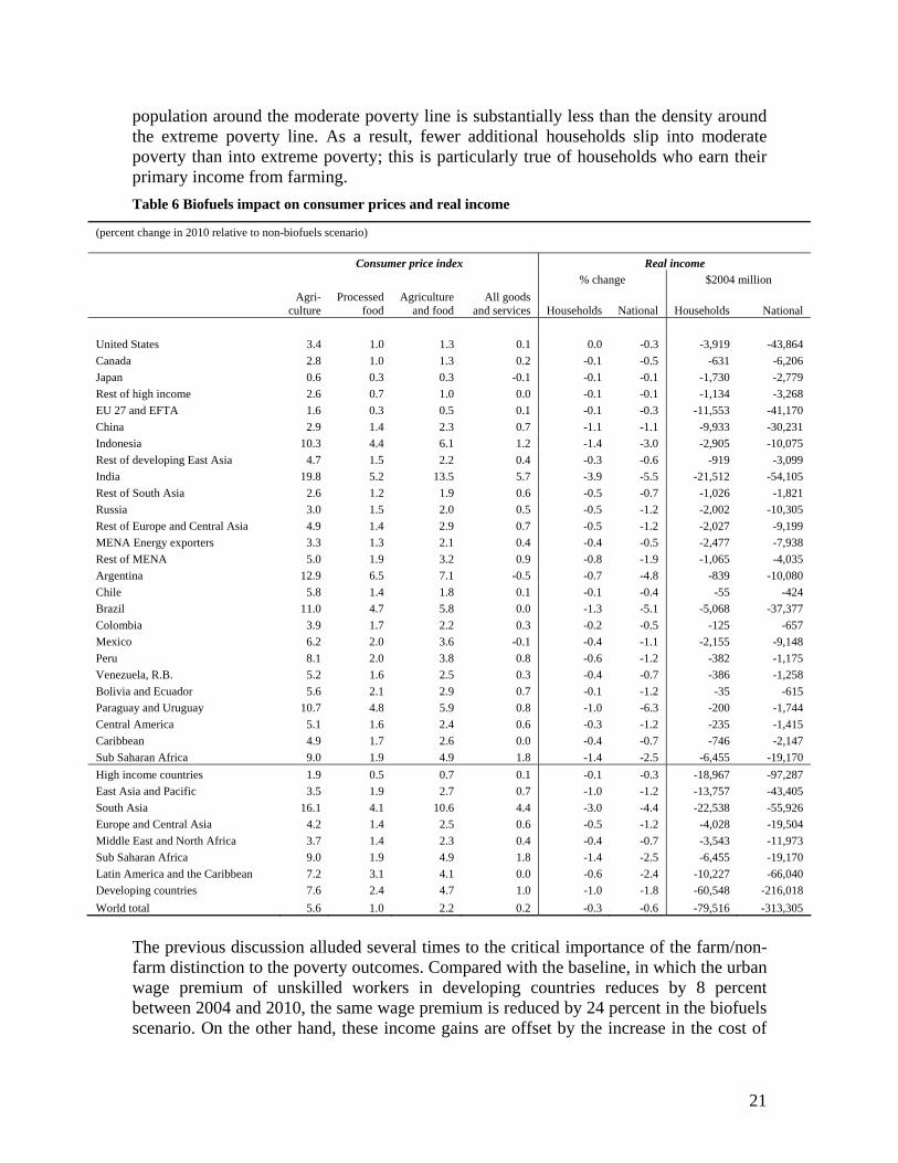
population around the moderate poverty line is substantially less than the density around the extreme poverty line. As a result, fewer additional households slip into moderate poverty than into extreme poverty; this is particularly true of households who earn their primary income from farming.

Table 6 Biofuels impact on consumer prices and real income

(percent change in 2010 relative to non-biofuels scenario)

Consumer price index Real income % change $2004 million

Agri-

culture Processed

food Agriculture

and food All goods

and services Households National Households National

United States 3.4 1.0 1.3 0.1 0.0 -0.3 -3,919 -43,864

Canada 2.8 1.0 1.3 0.2 -0.1 -0.5 -631 -6,206

Japan 0.6 0.3 0.3 -0.1 -0.1 -0.1 -1,730 -2,779

Rest of high income 2.6 0.7 1.0 0.0 -0.1 -0.1 -1,134 -3,268

EU 27 and EFTA 1.6 0.3 0.5 0.1 -0.1 -0.3 -11,553 -41,170

China 2.9 1.4 2.3 0.7 -1.1 -1.1 -9,933 -30,231

Indonesia 10.3 4.4 6.1 1.2 -1.4 -3.0 -2,905 -10,075

Rest of developing East Asia 4.7 1.5 2.2 0.4 -0.3 -0.6 -919 -3,099

India 19.8 5.2 13.5 5.7 -3.9 -5.5 -21,512 -54,105

Rest of South Asia 2.6 1.2 1.9 0.6 -0.5 -0.7 -1,026 -1,821

Russia 3.0 1.5 2.0 0.5 -0.5 -1.2 -2,002 -10,305

Rest of Europe and Central Asia 4.9 1.4 2.9 0.7 -0.5 -1.2 -2,027 -9,199

MENA Energy exporters 3.3 1.3 2.1 0.4 -0.4 -0.5 -2,477 -7,938

Rest of MENA 5.0 1.9 3.2 0.9 -0.8 -1.9 -1,065 -4,035

Argentina 12.9 6.5 7.1 -0.5 -0.7 -4.8 -839 -10,080

Chile 5.8 1.4 1.8 0.1 -0.1 -0.4 -55 -424

Brazil 11.0 4.7 5.8 0.0 -1.3 -5.1 -5,068 -37,377

Colombia 3.9 1.7 2.2 0.3 -0.2 -0.5 -125 -657

Mexico 6.2 2.0 3.6 -0.1 -0.4 -1.1 -2,155 -9,148

Peru 8.1 2.0 3.8 0.8 -0.6 -1.2 -382 -1,175

Venezuela, R.B. 5.2 1.6 2.5 0.3 -0.4 -0.7 -386 -1,258

Bolivia and Ecuador 5.6 2.1 2.9 0.7 -0.1 -1.2 -35 -615

Paraguay and Uruguay 10.7 4.8 5.9 0.8 -1.0 -6.3 -200 -1,744

Central America 5.1 1.6 2.4 0.6 -0.3 -1.2 -235 -1,415

Caribbean 4.9 1.7 2.6 0.0 -0.4 -0.7 -746 -2,147

Sub Saharan Africa 9.0 1.9 4.9 1.8 -1.4 -2.5 -6,455 -19,170

High income countries 1.9 0.5 0.7 0.1 -0.1 -0.3 -18,967 -97,287

East Asia and Pacific 3.5 1.9 2.7 0.7 -1.0 -1.2 -13,757 -43,405

South Asia 16.1 4.1 10.6 4.4 -3.0 -4.4 -22,538 -55,926

Europe and Central Asia 4.2 1.4 2.5 0.6 -0.5 -1.2 -4,028 -19,504

Middle East and North Africa 3.7 1.4 2.3 0.4 -0.4 -0.7 -3,543 -11,973

Sub Saharan Africa 9.0 1.9 4.9 1.8 -1.4 -2.5 -6,455 -19,170

Latin America and the Caribbean 7.2 3.1 4.1 0.0 -0.6 -2.4 -10,227 -66,040

Developing countries 7.6 2.4 4.7 1.0 -1.0 -1.8 -60,548 -216,018

World total 5.6 1.0 2.2 0.2 -0.3 -0.6 -79,516 -313,305

The previous discussion alluded several times to the critical importance of the farm/non-farm distinction to the poverty outcomes. Compared with the baseline, in which the urban wage premium of unskilled workers in developing countries reduces by 8 percent between 2004 and 2010, the same wage premium is reduced by 24 percent in the biofuels scenario. On the other hand, these income gains are offset by the increase in the cost of

21

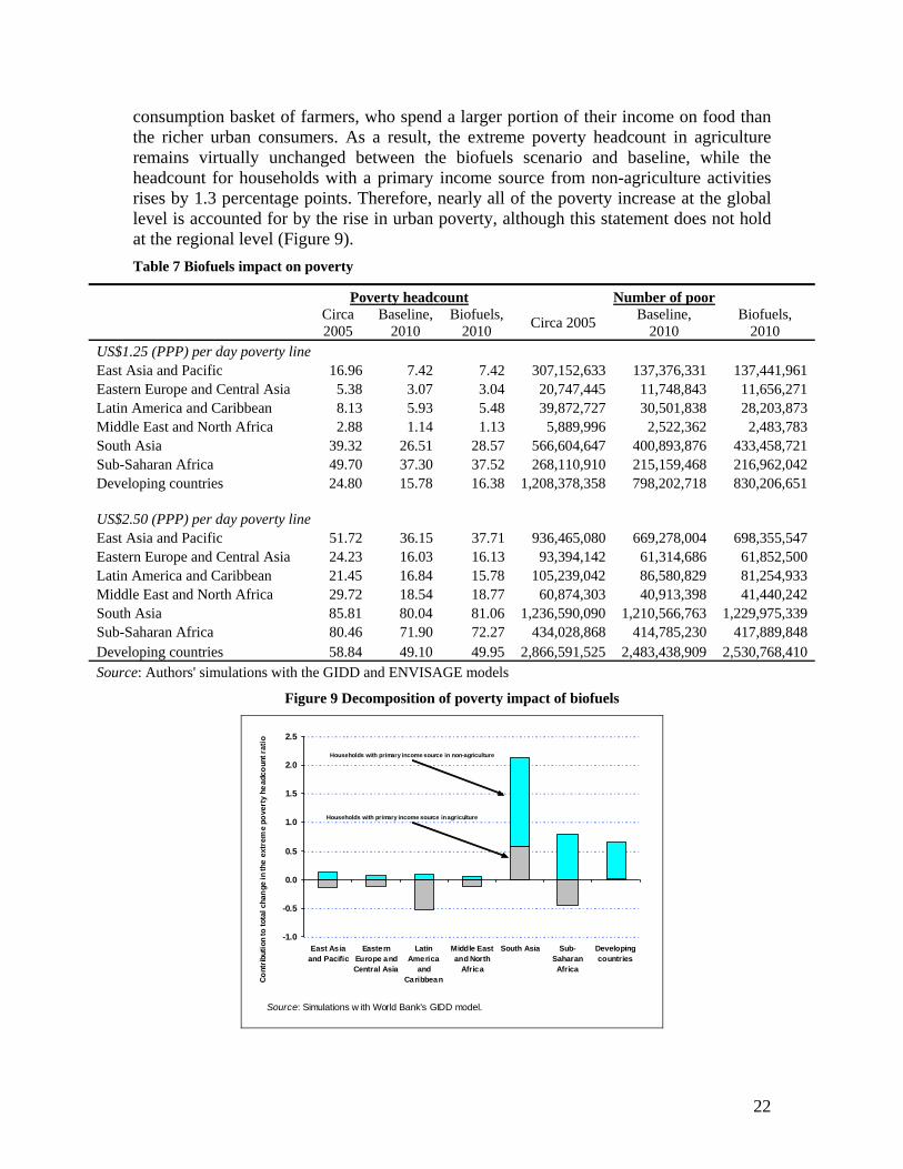
consumption basket of farmers, who spend a larger portion of their income on food than the richer urban consumers. As a result, the extreme poverty headcount in agriculture remains virtually unchanged between the biofuels scenario and baseline, while the headcount for households with a primary income source from non-agriculture activities rises by 1.3 percentage points. Therefore, nearly all of the poverty increase at the global level is accounted for by the rise in urban poverty, although this statement does not hold at the regional level (Figure 9).

Table 7 Biofuels impact on poverty

Poverty headcount Number of poor

Circa 2005

Baseline, 2010

Biofuels, 2010

Circa 2005 Baseline,

2010 Biofuels,

2010 US$1.25 (PPP) per day poverty line East Asia and Pacific 16.96 7.42 7.42 307,152,633 137,376,331 137,441,961 Eastern Europe and Central Asia 5.38 3.07 3.04 20,747,445 11,748,843 11,656,271 Latin America and Caribbean 8.13 5.93 5.48 39,872,727 30,501,838 28,203,873 Middle East and North Africa 2.88 1.14 1.13 5,889,996 2,522,362 2,483,783 South Asia 39.32 26.51 28.57 566,604,647 400,893,876 433,458,721 Sub-Saharan Africa 49.70 37.30 37.52 268,110,910 215,159,468 216,962,042 Developing countries 24.80 15.78 16.38 1,208,378,358 798,202,718 830,206,651 US$2.50 (PPP) per day poverty line East Asia and Pacific 51.72 36.15 37.71 936,465,080 669,278,004 698,355,547 Eastern Europe and Central Asia 24.23 16.03 16.13 93,394,142 61,314,686 61,852,500 Latin America and Caribbean 21.45 16.84 15.78 105,239,042 86,580,829 81,254,933 Middle East and North Africa 29.72 18.54 18.77 60,874,303 40,913,398 41,440,242 South Asia 85.81 80.04 81.06 1,236,590,090 1,210,566,763 1,229,975,339 Sub-Saharan Africa 80.46 71.90 72.27 434,028,868 414,785,230 417,889,848 Developing countries 58.84 49.10 49.95 2,866,591,525 2,483,438,909 2,530,768,410 Source: Authors' simulations with the GIDD and ENVISAGE models

Figure 9 Decomposition of poverty impact of biofuels

-1.0

-0.5

0.0

0.5

1.0

1.5

2.0

2.5

East Asiaand Pacific

EasternEurope andCentral Asia

LatinAmerica

andCaribbean

Middle Eastand North

Africa

South Asia Sub-Saharan

Africa

Developingcountries

Co

ntr

ibu

tion

to

to

tal

chan

ge

in t

he

ext

rem

e p

ove

rty

head

coun

t ra

tio

Source: Simulations w ith World Bank’s GIDD model.

Households with primary income source in non-agriculture

Households with primary income source in agriculture

22

6 Conclusions The spike in food prices between 2005 and the first half of 2008 has highlighted the vulnerabilities of poor consumers to higher prices of agricultural goods and has generated calls for massive policy action. This paper has provided a formal assessment of the first- and second-order implications of higher prices for global poverty using a representative sample of 63 to 93 percent of the population of the developing world. Using data on changes in the domestic food CPI over the period covering January 2005 and December 2007--when food prices increased by an average of 5.6 percent in real terms--the paper finds that the implied increase in the extreme poverty headcount at the global level is 1.7 percentage points. This estimate takes into account both the increase in the cost of each household’s food consumption basket and the rise in incomes of households that derive at least some of their earnings from the production of agricultural goods. The global number hides a significant amount of regional variation, with poverty in Eastern Europe and Central Asia and Latin America remaining roughly unchanged, while the headcount ratios in East Asia and the Middle East and North Africa increase by more than almost 6 and 2.4 percentage points, respectively. Although agricultural prices have declined from their mid-2008 highs, there are some indications that the long-term downward trend in the prices of agricultural commodities may be coming to an end, and thus the recent food crisis may be just a 'preview' of a world with higher food prices. By linking the household survey data with a general equilibrium model, the paper finds that a 5.5 percent increase in agricultural prices due to rising demand for first-generation biofuels could raise global poverty in 2010 by 0.6 percentage points at the extreme poverty line and 0.9 percentage points at the moderate poverty line. Poverty increases at the regional level vary substantially, with nearly all of the increase in extreme poverty occurring in South Asia and Sub-Saharan Africa. Although farmers benefit from higher output prices, they also tend to consume more food than the richer urban dwellers, which results in the agricultural poverty headcount remaining unchanged while the non-agriculture poverty headcounts increases by 1.3 percentage points. The results in this paper suggest that the poverty consequences of higher food prices are substantial, but that the implied total poverty elasticity of high prices (taking indirect effects into account) is much lower than the first-order, or direct, elasticity. Still, millions of consumers could fall into extreme poverty due to higher food prices, and millions more already under the poverty line are likely to experience a further deterioration in their living standards. The paper's results are dependent on a number of assumptions and estimated relationships--including food consumption shares in a number of countries, the share of self-employed income of agricultural households, structural features of the general equilibrium model, and the link between variables of the micro-simulation--and therefore should not be interpreted as the effect of higher food prices on poverty. The results nonetheless provide an important contribution to the discourse by identifying the relevant transmission channels, establishing the orders of magnitude, and exposing the regional and country variation concealed in the aggregate numbers.

23

References Aksoy, Ataman and Isik-Dikmelik, Aylin (2008) “Are Low Food Prices Pro-Poor? Net

Food Buyers and Sellers in Low-Income Countries”, World Bank Policy Research Working Paper No. 4642

Baffes, J. and Gardner, B. (2003) “The transmission of world commodity prices to

domestic markets under policy reforms in developing countries”, Journal of Economic Policy Reform, Volume 6, Issue 3 September 2003 , pages 159 – 180.

Bourguignon, François, Maurizio Bussolo, and Luiz A. Pereira da Silva (ed.) (2008),

“The Impact of Macroeconomic Policies on Poverty and Income Distribution: Macro–Micro Evaluation Techniques and Tools”, New York, NY: Palgrave.

Bussolo, M., De Hoyos, R. and Medvedev, D. (2008a) “Economic Growth and Income

Distribution: Linking Macroeconomic Models with Household Survey Data at the Global Level.” Paper presented at the International Association for Research in Income and Wealth (IARIW) 30th general conference, Portoroz, Slovenia, August 24-30.

Bussolo, M., De Hoyos, R. and Medvedev, D. (2009) “Global Income Distribution and

Poverty in the Absence of Agricultural Distortions”, in Anderson, K. (ed.) Distortions to Agricultural Incentives: A Global Perspective, London: Palgrave Macmillan and Washington DC: World Bank, forthcoming. Also World Bank Policy Research Working Paper 4849.

Bussolo, M., Lay, J. and van der Mensbrugghe, D. (2006) “Structural change and poverty

reduction in Brazil : the impact of the Doha Round.” World Bank Policy Research Working Paper 3833.

Carletto, G., Covarrubias, K., Davis, B., Krausova, M., Stamoulis, K., Winters, P., and

Zezza, A. (2007) “Rural Income Generating Activities in Developing Countries: Re-Assessing the Evidence”, Journal of Agricultural and Development Economics, vol. 4, No 1.

Chen, S. and Ravallion, M. (2003) “Household Welfare Impacts of China’s Accession to

the World Trade Organization.” World Bank Policy Research Working Paper 3040, Washington, DC

Chen, S. and Ravallion, M. (2008) “The Developing is Poorer than We Thought, But No

Less Successful in the Fight Against Poverty”, World Bank Policy Research Working Paper No. 4703, Washington, DC

24

Cline, W. R. (2007), “Global Warming and Agriculture: Impact Estimates by Country”, Center for Global Development and Peterson Institute for International Economics, Washington, DC.

Cranfield, J., Preckel, P., Eales, J. and Hertel, T. (2002) “Estimating consumer demands

across the development spectrum: maximum likelihood estimated of an implicit direct additivity model”, Journal of Development Economics, vol. 68, pg. 289-307

Deaton, Angus, (1989) “Rice Prices and Income Distribution in Thailand: A Non-

parametric Analysis,” Economic Journal, Royal Economic Society, vol. 99(395), pages 1-37

Dessus, S., Herrera, S., and de Hoyos, R. “The Impact of Food Inflation on Urban

Poverty and Its Monetary Cost: Some Back-of-the-Envelope Calculations”, World Bank Policy Research Working Paper, 4666, Washington, DC and (forthcoming) Agricultural Economics.

Friedman, J. and Levinsohn, J. (2002) “The distributional impacts of Indonesia’s

financial crisis on household welfare: a “rapid response” methodology” The World Bank Economic Review, vol. 16 No. 3

de Hoyos, R. and Lessem, R. (2008) “Food Shares in Consumption: New Evidence Using

Engel Curves for Developing Countries”, Background Paper for the Global Economic Prospects 2009, The World Bank

Ivanic, M. and Martin, W. (2008) “Implications of higher global food prices for poverty

in low income countries”, World Bank Policy Research Working Paper 4594, Washington, D.C

Levinsohn, J. (1996) “Competition Policy and International Trade”. In: Bhagwati, J. and

Hudec, R.E., (Eds.) Fair Trade and Harmonization: Prerequisites for Free Trade? Volumen One: Economic Analysis, 1st edition.

Martin, W. and Mitra, D. (1999) “Productivity Growth and Convergence in Agriculture

and Manufacturing,” World Bank Policy Research Working Paper 2171, Washington, DC.

Mitchell, D. (2008) “A Note on Rising Food Prices,” World Bank Policy Research

Working Paper 4682, Washington, DC. Nordhaus, W. (2007) “The Challenge of Global Warming: Economic Models and

Environmental Policy,” Yale University, New Haven, CT. Nordhaus, W. and Boyer, J. (2000) “Warming the World: Economic Models of Global

Warming”, MIT Press, Cambridge, MA.

25

Ravaillon, M. (1990), “Rural welfare changes of food prices under induced wage responses: theory and evidence from Bangladesh”, Oxford Economic Papers, 42, 574-85.

Ravallion, Martin and van de Walle, Dominique, (1991) “The impact on poverty of food

pricing reforms: A welfare analysis for Indonesia,” Journal of Policy Modeling, Elsevier, vol. 13(2), pages 281-299.

van der Mensbrugghe, D. (2008), “Environmental Impacts and Sustainability Applied

General Equilibrium (ENVISAGE) Model.” Washington, DC: World Bank. Wodon, Q., Tsimpo, C., Backiny-Yetna, P., Joseph, G., Adoho, F., and Coulombe, H.

(2008), “Measuring the potential impact of higher food prices on poverty: summary evidence from West and Central Africa”, mimeo, May, World Bank, Washington D.C.

World Bank (2009) “Global Economic Prospects 2009: Commodities and Developing

Economies”, Washington DC.

26

Annex I

Table 8 ENVISAGE dimensions

Regions Sectors United States MENA Energy exporters Paddy rice Other mining Canada Rest of MENA Wheat Processed food Japan Brazil Other cereal grains Refined oil Rest of high income Mexico Oil seeds Chemicals etc. Western Europe Colombia Sugar cane and beet Energy int. manu. China Peru Other crops Other manufacturing Indonesia Venezuela, R.B. Livestock Electricity Rest of Dev. East Asia Argentina Forestry Gas distribution India Chile Coal Construction Rest of South Asia Bolivia and Ecuador Crude oil Transport services Russia Paraguay & Uruguay Natural gas Other services Rest of ECA Central America Sub Saharan Africa Caribbean

27

Annex II Table 9: Country composition of the GIDD dataset

Region Covered population Actual population Covered Population (%)

World 5,498,162 6,076,509 90.48East Asia and Pacific 1,733,358 1,817,232 95.38Eastern Europe and Central Asia 460,385 471,549 97.63High Income Countries 764,285 974,612 78.42Latin America 500,199 515,069 97.11Middle East and North Africa 190,397 276,447 68.87South Asia 1,332,800 1,358,294 98.12Sub-Saharan Africa 516,737 663,305 77.90

Economy Covered population Actual population Data used

East Asia and Pacific 1,733,358 1,805,691 China 1,260,000 1,260,000 grouped Indonesia 212,000 212,000 individual Vietnam 80,400 80,400 individual Philippines 71,600 71,600 individual Thailand 61,700 61,700 individual Malaysia 23,300 23,300 grouped Cambodia 11,900 11,900 individual Lao PDR 4,927 4,927 individual Papua New Guinea 5,133 5,133 grouped Mongolia 2,398 2,398 grouped Myanmar 47,700 Korea, Dem. Rep. 21,900 Fiji 811 Timor-Leste 784 Solomon Islands 419 Vanuatu 191 Samoa 177 Micronesia, Fed. Sts. 107 Tonga 100 Kiribati 91 Marshall Islands 53 Eastern Europe and Central Asia 460,385 471,549 Russian Federation 136,000 146,000 individual Turkey 69,600 67,400 individual Ukraine 47,600 49,200 individual Poland 38,300 38,500 individual Uzbekistan 25,100 24,700 individual Romania 21,800 22,400 individual Kazakhstan 15,000 14,900 individual Serbia and Montenegro 10,600 8,137 grouped Czech Republic 10,300 10,300 grouped Hungary 9,876 10,200 individual Belarus 9,994 10,000 individual Azerbaijan 8,199 8,049 individual Bulgaria 7,906 8,060 individual Tajikistan 6,376 6,159 individual Slovak Republic 5,393 5,389 grouped

28

Georgia 4,514 4,720 individual Kyrgyz Republic 5,008 4,915 individual Turkmenistan 4,644 4,502 grouped Croatia 4,446 4,503 grouped Moldova 4,259 4,275 individual Lithuania 3,477 3,500 individual Armenia 3,065 3,082 individual Albania 3,139 3,062 individual Latvia 2,383 2,372 grouped Estonia 1,363 1,370 individual Macedonia, FYR 2,044 2,010 individual Bosnia and Herzegovina 3,847 High Income Countries 764,285 974,612 United States 282,000 282,000 grouped Germany 82,200 82,200 grouped France 58,900 58,900 grouped United Kingdom 58,800 59,700 grouped Italy 57,700 56,900 grouped Korea, Rep. 47,000 47,000 grouped Spain 40,500 40,300 grouped Canada 30,800 30,800 grouped Netherlands 15,900 15,900 grouped Greece 10,900 10,900 grouped Belgium 10,300 10,300 grouped Portugal 10,100 10,200 grouped Sweden 8,875 8,869 grouped Austria 8,011 8,012 grouped Hong Kong, China 6,669 6,665 grouped Israel 6,282 6,289 grouped Denmark 5,338 5,337 grouped Finland 5,177 5,176 grouped Norway 4,492 4,491 grouped Singapore 4,020 4,018 grouped New Zealand 3,864 3,858 grouped Ireland 3,815 3,805 grouped Slovenia 1,986 1,989 grouped Luxembourg 441 438 grouped Netherlands Antilles 215 176 grouped Japan 127,000 Taiwan, China 22,200 Saudi Arabia 20,700 Australia 19,200 Switzerland 7,184 Puerto Rico 3,816 United Arab Emirates 3,247 Kuwait 2,190 Cyprus 694 Bahrain 672 Qatar 606 Macao, China 444 Malta 390 Brunei Darussalam 333 Bahamas, The 301 Iceland 281

29

French Polynesia 236 New Caledonia 213 Guam 155 Channel Islands 147 Virgin Islands (U.S.) 109 Antigua and Barbuda 76 Isle of Man 76 Bermuda 62 Greenland 56 Latin America 500,199 515,069 Brazil 172,000 174,000 individual Mexico 98,000 98,000 individual Colombia 41,600 42,100 individual Argentina 37,300 36,900 individual Peru 26,800 26,000 individual Venezuela, RB 24,300 24,300 individual Chile 15,200 15,400 individual Ecuador 12,000 12,300 individual Guatemala 11,800 11,200 individual Bolivia 8,514 8,317 individual Dominican Republic 7,950 8,265 individual Haiti 8,146 7,939 individual Honduras 6,281 6,424 individual El Salvador 6,409 6,280 individual Paraguay 5,386 5,346 individual Nicaragua 5,186 4,920 individual Costa Rica 3,805 3,929 individual Uruguay 3,332 3,342 individual Panama 2,849 2,950 individual Jamaica 2,607 2,589 individual Guyana 733 744 individual Cuba 11,100 Trinidad and Tobago 1,285 Suriname 434 Barbados 266 Belize 250 St. Lucia 156 St. Vincent and the Grenadines 116 Grenada 101 Dominica 71 St. Kitts and Nevis 44 Middle East and North Africa 190,397 276,447 Egypt, Arab Rep. 67,300 67,300 grouped Iran, Islamic Rep. 63,700 63,700 grouped Morocco 27,800 27,800 individual Yemen, Rep. 16,500 17,900 individual Tunisia 9,565 9,564 grouped Jordan 5,532 4,857 individual Algeria 30,500 Iraq 23,200 Syrian Arab Republic 16,800 Libya 5,306 Lebanon 3,398 West Bank and Gaza 2,966

30

Oman 2,442 Djibouti 715 South Asia 1,332,800 1,358,294 India 1,020,000 1,020,000 individual Pakistan 142,000 138,000 individual Bangladesh 131,000 129,000 individual Nepal 20,800 24,400 individual Sri Lanka 19,000 19,400 individual Afghanistan 26,600 Bhutan 604 Maldives 290 Sub-Saharan Africa 516,737 663,305 Nigeria 137,000 118,000 individual Ethiopia 64,300 64,300 individual South Africa 43,900 44,000 individual Tanzania 34,500 34,800 individual Kenya 28,100 30,700 individual Uganda 24,600 24,300 individual Ghana 19,300 19,900 individual Côte d'Ivoire 16,500 16,700 individual Madagascar 16,000 16,200 individual Cameroon 15,500 14,900 individual Zimbabwe 12,600 12,600 grouped Zambia 12,600 10,700 grouped Niger 11,800 11,800 grouped Mali 11,100 11,600 individual Burkina Faso 10,800 11,300 individual Malawi 10,300 11,500 grouped Rwanda 8,024 8,025 grouped Guinea 7,929 8,434 individual Senegal 7,914 10,300 individual Benin 6,718 7,197 individual Burundi 6,563 6,486 individual Sierra Leone 4,509 4,509 grouped Mauritania 2,668 2,645 individual Lesotho 1,743 1,788 grouped Gambia, The 1,217 1,316 individual Comoros 554 540 grouped Congo, Dem. Rep. 50,100 Sudan 32,900 Mozambique 17,900 Angola 13,800 Chad 8,216 Somalia 7,012 Togo 5,364 Central African Republic 3,777 Eritrea 3,557 Congo, Rep. 3,438 Liberia 3,065 Namibia 1,894 Botswana 1,754 Guinea-Bissau 1,366 Gabon 1,272 Mauritius 1,187

31

32

Swaziland 1,045 Cape Verde 451 Equatorial Guinea 449 São Tomé and Principe 140 Seychelles 81

poverty effects of higher food prices

Documents