Institute of Actuaries of Australia ABN 69 000 423 656

Level 2, 50 Carrington Street, Sydney NSW Australia 2000

t +61 (0) 2 9239 6100 f +61 (0) 2 9239 6170

e actuaries@actuaries.asn.au w www.actuaries.asn.au

Building better PPAC models

Prepared by Hugh Miller

Presented to the Actuaries Institute

Injury & Disability Schemes Seminar

12 – 14 November 2017

November

This paper has been prepared for the Actuaries Institute 2017 Injury Schemes Seminar.

The Institute’s Council wishes it to be understood that opinions put forward herein are not necessarily those of the

Institute and the Council is not responsible for those opinions.

Hugh Miller

The Institute will ensure that all reproductions of the paper acknowledge the

author(s) and include the above copyright statement.

Building better PPAC models

Hugh Miller∗

Abstract

While generalised linear models (GLMs) have achieved some level of ac-ceptance in actuarial work, many reserving problems are still performed usingtraditional approaches in spreadsheets. A large part of this is that the per-ceived extra value from using a GLM is low, combined with the uncertaintyof how a GLM compares to a traditional approach. This paper argues thatthe GLM approach is preferable, containing virtually all of the benefits ofa traditional model and also permitting powerful extensions and improve-ments. These improvements to models using GLMs are largely unreportedin the academic literature. The discussion is supported with theoretical andsimulation results.

The paper focuses primarily on the PPAC model (payments per activeclaim), a very common valuation technique for long-tailed liabilities.

Keywords: Payments per active claim models; Generalised linear models; Activeclaims; Chain ladder; Reserving

1 Introduction

The last few decades has seen many changes in actuarial work due to the improve-ments in computational power and software. One area where this has met someresistance is the use of generalised linear models (or GLMs; see McCullagh & Nelder,1989, and Dobson, 2002) to replace traditional models such as the the chain ladderfor reserving triangles. Reserving triangles remain a key part of non-life insurance.There are a number of legitimate reasons for this resistance:

• Traditional average methods can be easily performed in spreadsheet softwaresuch as Microsoft Excel. This means the dataset, assumptions and forecastare easy to inspect simultaneously; changes to assumptions can be easily madeand their impacts quickly seen; the model is interpretable to other users;

• Traditional average methods are seen to be relatively fast to implement.

• The “value-add” from using a generalised linear model is often unclear, par-ticularly to non-technical users of reserving estimates.

• There are some practical issues with using GLMs, including treatment of zerosin the data and the ability to impose prior knowledge on model parameters.

• A familiarity bias, where conversion to a GLM can appear daunting to actu-aries not experienced with linear models.

∗Correspondence to: Hugh Miller, Taylor Fry, Level 22, 45 Clarence St, Sydney, 2000, Australia.Email: hugh.miller@taylorfry.com.au

1

This paper discusses the use of GLMs for these types of reserving models. Itprimarily focuses the third and fourth items listed above; GLMs can do everythinga traditional model can do, plus more, and many of the practical issues can beovercome. However the other items are also addressed, arguing that properly im-plemented GLMs can be easy to use and standard fits can be implemented quickly.

To make the discussion concrete, a specific type of model, the “payment peractive claim” or PPAC model will be discussed. This has been chosen due toits common use in modelling long tailed benefits such as workers’ compensation, adifficult class for reserving. Most of the comments are applicable to other traditionalactuarial reserving models.

This paper is primarily pedagogical; it seeks to be practical in applying GLMsto reserving problems, bridging actuarial theory and practice. However, there aresome novelties. Most of the ideas in Section 4 are new to the actuarial literature.Further, some claims as to best practice are supported by theoretical results in thetechnical appendix.

The remainder of the paper is structured as follows. Section 2 introduces PPACmodels, GLMs and example datasets in some detail. Section 3 discusses some ofthe considerations for all types of PPAC models. Section 4 covers a number ofadditional considerations for when PPAC models are built using GLMs. Section 5provides some further discussion and conclusions. Finally, the theoretical appendixprovides some statistical results that underlie some of the discussion throughoutthe paper.

2 Background

2.1 Data We assume a triangle of historical data, with rows representing accidentyears i = 1, . . . , I, columns development years j = 1, . . . , J and payment yeark = i + j = 1, . . . , K. The general aim of loss reserving aim is to “complete thetriangle”, to determine payments that will occur in the future related to accidentsincurred in the past. For each cell in the triangle we have two pieces of information;the number of people “active” on that benefit, nij, and the amount of payments,Qij. Payments are often inflation-adjusted at the beginning of the analysis. Whilethe definition of active can vary depending on context, one simple and oft-useddefinition is the presence of any payment in that year.

The chosen interval above is years, but this is of course arbitrary and differenttime increments can be adopted. Other possible extensions to the data, not pursuedin this paper, include:

• The inclusion of other claimant variables. One obvious example is claimantage, as different ages have different rates of continuance on benefit as wellas permitting explicit retirement or death decrements if desired. If age wereadded, then each cell of data (i, j) is split into multiple observations; one foreach observed age group in the cell.

• The inclusion of other time related variables. The behaviour of beneficiariesis often correlated to macro-economic variables such as unemployment rates

2

or growth in GDP. These are relatively straightforward to “attach” thesemodelling variables to the appropriate diagonals.

2.2 PPAC models The payment per active claim is defined as total payments inthe cell divided by the number of active claims

Pij = Qij/nij (2.1)

A PPAC based valuation is then made up of two models, described below.The continuance rate model relates to the rate at which active claims become

inactive or closed. It involves the estimation of continuance rate factors cj, whichare typically assumed to vary by development period but not by accident year.

nij ≈ cjni,j−1 (2.2)

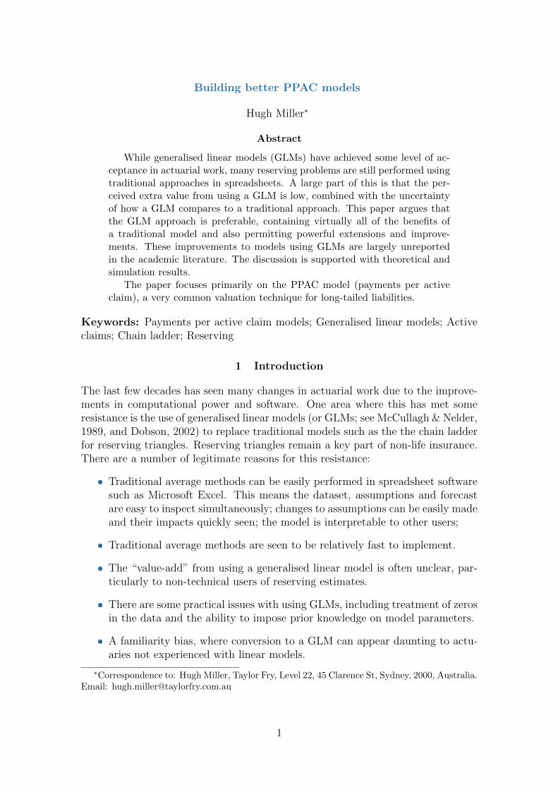
The cj are estimated based on historical ratios of nij/ni,j−1 across the various acci-dent years i. In practice the observed continuance rates will not always be constantacross accidents years, either due to random fluctuations or systematic evolutionover time. For this reason we express equation (2.2) as approximate. Noise is gen-erally dealt with via averaging continuance rates over a number of accident periods,while systematic evolution requires some assessment of the trend before selecting cjfor future periods.

The payment model relates to the average payment level per active claim. Again,these factors Pj is typically assumed to vary by development period but not byaccident year.

Pj ≈ Pij =Qij

nij

(2.3)

Observed payment levels will not necessarily be constant down a column of thetriangle due to both noise and systematic effects. The most common systematiceffect is superimposed inflation (SI), where succcessive payment years (diagonals)tend to see increases.

PPAC models have proven to be a popular form of reserving model, allowingcareful study of numbers of active claims, and are useful where there are consistentlysized payments made over an extended period of time. They are used in manycountries, but are particularly popular in Australia to value long term injury claimssuch as workers’ compensation.

PPACs are but one example of reserving triangles, which have been studiedextensively in the actuarial literature. Taylor (1986) gives an overview of earlywork on reserving triangles. The Mack (1993) model established a distribution-freeformula for the standard error of chain ladder reserves. England & Verall (2002)extended this to a fuller framework of stochastic claim reserving. The textbook byTaylor (2000) gives a relatively modern theoretical overview to loss reserving.

3

Accident

Year 0 1 2 3 4 5 6 7 8 9 10 11 12 13 14 15 16 17 18

1995 105 73 55 47 38 35 33 31 30 29 29 29 29 29 28 27 26 22 22

1996 110 77 56 43 38 33 31 31 31 31 29 29 27 27 25 25 24 24 23.3

1997 115 85 63 55 50 42 41 40 40 39 37 37 35 35 35 33 32 31.0 30.1

1998 120 85 67 52 41 34 31 29 28 26 26 26 25 25 25 23 22.3 21.6 21.0

1999 126 87 68 50 42 40 38 33 32 31 30 30 29 29 28 27.2 26.3 25.6 24.8

2000 132 85 63 52 48 40 39 37 36 35 35 34 33 31 30.1 29.2 28.3 27.4 26.6

2001 138 94 78 59 48 45 45 43 40 37 36 36 36 34.9 33.9 32.9 31.9 30.9 30.0

2002 144 97 72 60 52 44 43 41 40 40 39 39 38.1 36.9 35.8 34.7 33.7 32.7 31.7

2003 151 112 80 61 54 50 49 46 45 44 42 41.7 40.7 39.5 38.3 37.2 36.0 35.0 33.9

2004 158 114 91 77 63 55 52 49 46 46 44.8 44.5 43.4 42.1 40.9 39.6 38.5 37.3 36.2

2005 165 112 89 75 62 54 51 48 47 45.9 44.7 44.4 43.3 42.0 40.8 39.6 38.4 37.2 36.1

2006 173 113 87 72 58 49 46 43 41.6 40.6 39.6 39.3 38.4 37.2 36.1 35.0 34.0 32.9 32.0

2007 181 129 105 88 74 66 63 59.2 57.3 55.9 54.5 54.1 52.8 51.2 49.7 48.2 46.7 45.3 44.0

2008 190 131 103 75 63 57 53.9 50.7 49.0 47.9 46.7 46.3 45.2 43.9 42.5 41.3 40.0 38.8 37.7

2009 199 137 106 79 66 58.0 54.9 51.6 49.9 48.8 47.5 47.2 46.0 44.7 43.3 42.0 40.8 39.5 38.3

2010 208 138 104 90 74.8 65.8 62.3 58.5 56.6 55.3 53.8 53.5 52.2 50.6 49.1 47.6 46.2 44.8 43.5

2011 218 144 104 82.6 68.7 60.4 57.1 53.7 51.9 50.7 49.4 49.1 47.9 46.5 45.1 43.7 42.4 41.1 39.9

2012 228 156 118.3 93.9 78.1 68.7 65.0 61.0 59.1 57.7 56.2 55.8 54.5 52.8 51.2 49.7 48.2 46.8 45.4

2013 239 161.1 122.1 97.0 80.6 70.9 67.1 63.0 61.0 59.6 58.0 57.6 56.3 54.6 52.9 51.3 49.8 48.3 46.9

Continuance rate calculations

All 0.6882 0.7672 0.8042 0.8434 0.8810 0.9574 0.9439 0.9696 0.9728 0.9712 0.9962 0.9683 0.9888 0.9724 0.9558 0.9647 0.9200 1.0000

Last 4 0.6741 0.7582 0.7943 0.8312 0.8794 0.9464 0.9394 0.9674 0.9766 0.9744 0.9929 0.9762 0.9836 0.9741 0.9558 0.9647 0.9200 1.0000

Last 2 0.6726 0.7376 0.8048 0.8377 0.8978 0.9478 0.9381 0.9588 0.9890 0.9643 1.0000 0.9857 0.9677 0.9815 0.9333 0.9655 0.9200 1.0000

Selected 0.6741 0.7582 0.7943 0.8312 0.8794 0.9464 0.9394 0.9674 0.9766 0.9744 0.9929 0.9762 0.9700 0.9700 0.9700 0.9700 0.9700 0.9700

Development year

Table 1: Chain ladder continuance rate model, synthetic data

4

Accident

Year 0 1 2 3 4 5 6 7 8 9 10 11 12 13 14 15 16 17 18

1995 1,000 2,275 2,287 2,752 2,264 2,460 2,627 3,350 2,780 4,653 4,333 3,220 3,569 3,966 4,244 3,995 4,950 5,231 4,075

1996 1,131 2,190 2,269 2,102 2,647 2,464 2,489 2,878 3,318 4,139 2,807 4,083 3,665 4,602 4,417 4,313 5,132 4,774 4,075

1997 1,189 2,122 2,335 2,094 3,370 2,808 2,880 3,008 3,266 3,805 3,961 3,567 4,417 3,924 4,520 4,772 4,441 4,993 4,075

1998 1,166 2,511 2,284 2,244 2,550 2,942 2,878 3,157 3,070 3,759 3,835 4,554 3,511 4,612 4,726 4,810 4,805 4,993 4,075

1999 687 2,091 2,726 2,599 3,853 2,973 3,223 4,261 3,379 3,983 3,485 4,059 4,246 4,851 4,086 4,480 4,805 4,993 4,075

2000 940 2,381 2,718 2,389 3,425 3,110 3,499 3,332 3,290 3,890 4,274 4,738 3,983 4,678 4,435 4,480 4,805 4,993 4,075

2001 1,355 2,732 2,758 2,768 3,204 3,207 3,492 3,401 3,964 4,004 4,499 4,266 3,904 4,486 4,435 4,480 4,805 4,993 4,075

2002 1,195 2,453 3,230 3,344 3,077 3,291 3,539 3,865 4,379 4,032 4,120 4,472 3,926 4,486 4,435 4,480 4,805 4,993 4,075

2003 922 2,509 2,600 3,146 3,428 3,215 3,447 4,529 4,167 4,215 4,695 4,394 3,926 4,486 4,435 4,480 4,805 4,993 4,075

2004 1,307 2,577 2,965 3,201 3,147 3,760 3,564 3,665 3,685 4,706 4,404 4,394 3,926 4,486 4,435 4,480 4,805 4,993 4,075

2005 1,528 2,899 3,055 3,170 3,147 4,245 4,062 3,435 4,198 4,260 4,404 4,394 3,926 4,486 4,435 4,480 4,805 4,993 4,075

2006 1,236 2,823 3,193 3,735 3,735 3,894 3,745 4,171 4,098 4,260 4,404 4,394 3,926 4,486 4,435 4,480 4,805 4,993 4,075

2007 1,517 2,862 3,105 3,227 3,249 4,132 4,088 3,936 4,098 4,260 4,404 4,394 3,926 4,486 4,435 4,480 4,805 4,993 4,075

2008 1,666 3,152 3,041 3,386 3,392 3,911 3,879 3,936 4,098 4,260 4,404 4,394 3,926 4,486 4,435 4,480 4,805 4,993 4,075

2009 1,632 2,773 3,524 3,754 4,041 4,052 3,879 3,936 4,098 4,260 4,404 4,394 3,926 4,486 4,435 4,480 4,805 4,993 4,075

2010 1,599 3,148 3,146 3,520 3,592 4,052 3,879 3,936 4,098 4,260 4,404 4,394 3,926 4,486 4,435 4,480 4,805 4,993 4,075

2011 1,658 3,165 3,321 3,468 3,592 4,052 3,879 3,936 4,098 4,260 4,404 4,394 3,926 4,486 4,435 4,480 4,805 4,993 4,075

2012 1,658 3,954 3,260 3,468 3,592 4,052 3,879 3,936 4,098 4,260 4,404 4,394 3,926 4,486 4,435 4,480 4,805 4,993 4,075

2013 1,631 3,281 3,260 3,468 3,592 4,052 3,879 3,936 4,098 4,260 4,404 4,394 3,926 4,486 4,435 4,480 4,805 4,993 4,075

Payment per active claim, no superimposed inflation assumption. Averages are volume weighted

All 1,376 2,791 2,926 3,059 3,282 3,418 3,435 3,621 3,656 4,135 4,051 4,127 3,925 4,418 4,397 4,480 4,805 4,993 4,075

Last 4 1,637 3,281 3,260 3,468 3,592 4,052 3,879 3,936 4,098 4,260 4,404 4,394 3,926 4,486 4,435 4,480 4,805 4,993 4,075

Last 2 1,645 3,575 3,233 3,629 3,724 4,030 3,943 3,783 3,944 4,466 4,418 4,373 3,942 4,762 4,388 4,787 4,737 4,993 4,075

Selected 3,281 3,260 3,468 3,592 4,052 3,879 3,936 4,098 4,260 4,404 4,394 3,926 4,486 4,435 4,480 4,805 4,993 4,075

Development year

Table 2: Payments model, synthetic data

5

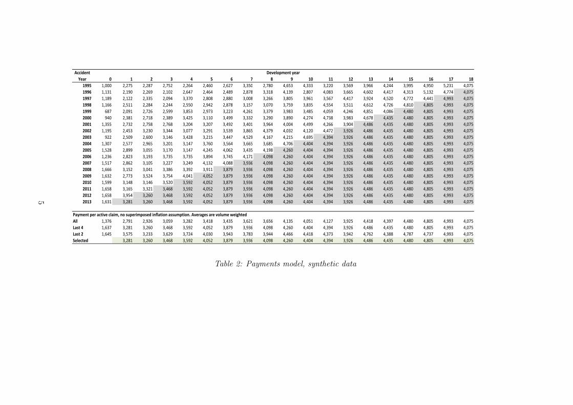
2.3 Traditional spreadsheet PPAC implementations Much of the current practiceof these types of models still use chain ladder based approaches. Tables 1 and 2show an example of this on a synthetic dataset. We carry this example throughthe paper for concreteness. In each table the upper triangle is historical, while thelower half are projections based on the selections for continuance rates (cj) andpayment level (Pj). The projected numbers of actives and payment levels can thenbe multiplied to obtain all projected future cash flows. We make a few additionalcomments about the example:

• The “All” continuance rate estimates are the overall (volume-weighted) aver-age continuances for all historical entries in the column. If H denotes the setof i, j that are historical (i+ j are equal to or less than the current paymentyear) then the estimate is:

cj =

∑i:(i,j)∈H nij∑

i:(i,j)∈H ni,j−1, for j ≥ 1. (2.4)

The “Last 4” estimate for cj is the equivalent sum, but only using the fourmost recent diagonals, so for instance the first number in the row is calculatedas

137 + 138 + 144 + 156

199 + 208 + 218 + 228= 0.6741 .

Similarly “Last 2” uses the last two diagonals. The use of “Last X” averagesis a very common way to have the adopted factors emphasise the most recenttrends. The projected values use the last 4 average for the projection fordevelopment periods 1 to 12.

• The 0.97 selected for development periods 13 to 18. It is common to “pool”averages across development periods, particularly in averages of higher uncer-tainty (continuance rates close to 1, or low numbers of observed claims).

• While not done here, it is common practice to “smooth” the leading diagonal(with reference to prior observations in the row). This reflects a belief thatunusually high (or low) continuance in a cell is often followed by reversion vialower (or higher) continuance thereafter.

• The projection of actives starts from the leading diagonal and applies theselected continuance factor assumptions according to Equation 2.2.

• The “All” payment level rates use a (volume-weighted) average:

Pj =

∑i:(i,j)∈H Pijnij∑i:(i,j)∈H nij

. (2.5)

The “last X” rows are the equivalent averages using only the last few rows ofdata. Again, this is common practice to emphasise recent trends.

• There appears to be superimposed inflation present in the payments triangle,with earlier rows appearing lower than cells below. The selection shown inTable 2 does not allow for this feature, but we discuss superimposed inflationin Section 4.2.

6

• There are a significant number of active claims at development year 18. Inpractice the projection would be extended to some larger number of develop-ment periods to estimate payments in the tail of the liability. Continuance andpayment level assumptions would generally be extrapolated from the latestobserved development periods.

2.4 GLMs for PPAC models A GLM for continuance rate modelling is a typicallya model of the form:

cij = g−1(XTijβ) + error , (2.6)

where

Xij = p-vector of predictors (or covariates) corresponding to cell (i, j)

g−1 = the inverse of the link function. The log-link g−1() = exp(), is common

to ensure positive continuance rates

error = An error term with zero mean

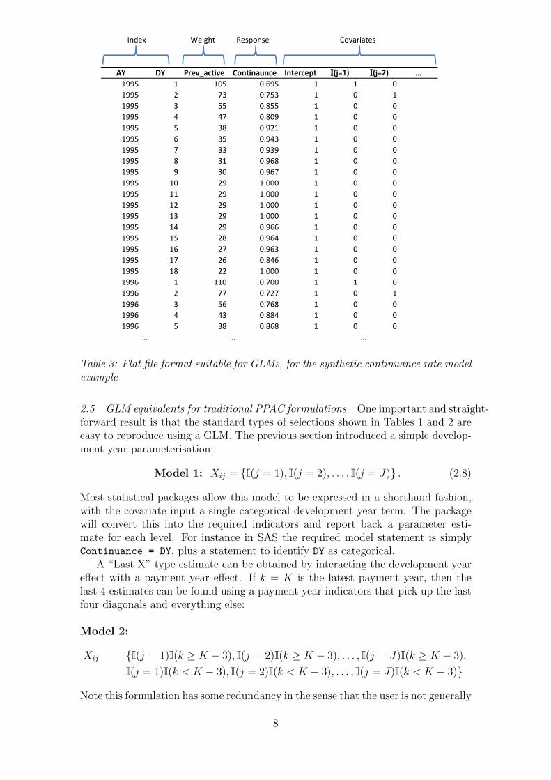
The response of a GLM (and thus the distribution of the error term) is assumedto be taken from the exponential family of distributions (see Fahrmeier & Tutz,1994 or Clark & Thayer, 2004), which will then determine the distribution for theerror term. The β are then estimated by maximum likelihood. It is common forthe first element of Xij to equal 1 for all i, j combinations, corresponding to anintercept term. A input dataset for a GLM has one row per “observation”, so thedata triangle must be converted into a flat file - see Table 3 for an example layout ofthe synthetic continuance rate triangle with illustrative covariates. A weight termfor each observation wij can be included in the maximum likelihood calculation toreflect the relative importance of each observation. For continuance rate modelsthe number of active claims in the previous year, wij = ni,j−1, forms a naturalweight. This choice of weight produces volume-weighted estimates of the type seenin Section 2.3

Of particular interest to this paper is the choice of covariates for the model. LetI(A) be the indicator function that takes the value 1 if A is true and zero otherwise.If :

Xij = {I(j = 1), I(j = 2), . . . , I(j = J)} ,

then one parameter estimate will be made for each development period. This setuphas the useful property of recovering the average chain ladder continuance factorscalculated in Table 1 (see also Result 1 in the technical appendix for the proof).

The GLM for payment levels is very similar in application:

Pij = g−1(XTijβ) + error , (2.7)

A good default weight is wij = nij, the number of active claims.

7

AY DY Prev_active Continaunce Intercept IIII(j=1) IIII(j=2) …

1995 1 105 0.695 1 1 0

1995 2 73 0.753 1 0 1

1995 3 55 0.855 1 0 0

1995 4 47 0.809 1 0 0

1995 5 38 0.921 1 0 0

1995 6 35 0.943 1 0 0

1995 7 33 0.939 1 0 0

1995 8 31 0.968 1 0 0

1995 9 30 0.967 1 0 0

1995 10 29 1.000 1 0 0

1995 11 29 1.000 1 0 0

1995 12 29 1.000 1 0 0

1995 13 29 1.000 1 0 0

1995 14 29 0.966 1 0 0

1995 15 28 0.964 1 0 0

1995 16 27 0.963 1 0 0

1995 17 26 0.846 1 0 0

1995 18 22 1.000 1 0 0

1996 1 110 0.700 1 1 0

1996 2 77 0.727 1 0 1

1996 3 56 0.768 1 0 0

1996 4 43 0.884 1 0 0

1996 5 38 0.868 1 0 0

… … …

Index Weight Response Covariates

Table 3: Flat file format suitable for GLMs, for the synthetic continuance rate modelexample

2.5 GLM equivalents for traditional PPAC formulations One important and straight-forward result is that the standard types of selections shown in Tables 1 and 2 areeasy to reproduce using a GLM. The previous section introduced a simple develop-ment year parameterisation:

Model 1: Xij = {I(j = 1), I(j = 2), . . . , I(j = J)} . (2.8)

Most statistical packages allow this model to be expressed in a shorthand fashion,with the covariate input a single categorical development year term. The packagewill convert this into the required indicators and report back a parameter esti-mate for each level. For instance in SAS the required model statement is simplyContinuance = DY, plus a statement to identify DY as categorical.

A “Last X” type estimate can be obtained by interacting the development yeareffect with a payment year effect. If k = K is the latest payment year, then thelast 4 estimates can be found using a payment year indicators that pick up the lastfour diagonals and everything else:

Model 2:

Xij = {I(j = 1)I(k ≥ K − 3), I(j = 2)I(k ≥ K − 3), . . . , I(j = J)I(k ≥ K − 3),

I(j = 1)I(k < K − 3), I(j = 2)I(k < K − 3), . . . , I(j = J)I(k < K − 3)}

Note this formulation has some redundancy in the sense that the user is not generally

8

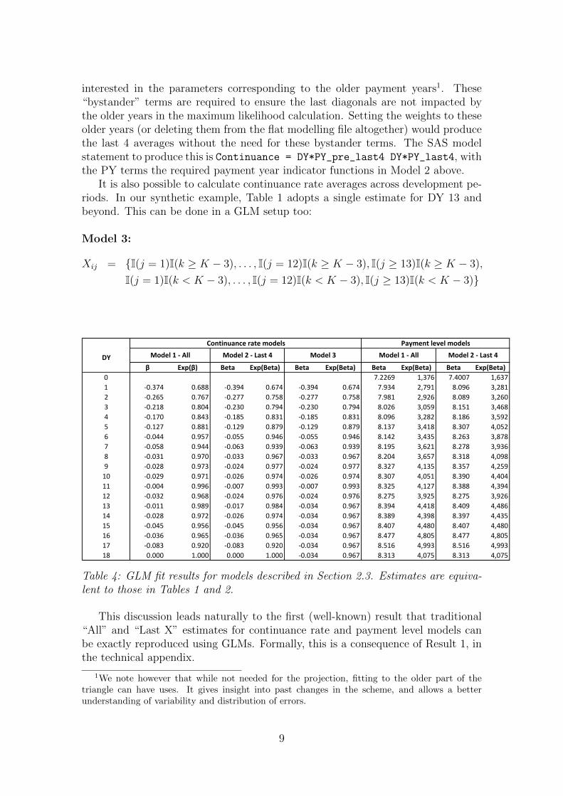
interested in the parameters corresponding to the older payment years1. These“bystander” terms are required to ensure the last diagonals are not impacted bythe older years in the maximum likelihood calculation. Setting the weights to theseolder years (or deleting them from the flat modelling file altogether) would producethe last 4 averages without the need for these bystander terms. The SAS modelstatement to produce this is Continuance = DY*PY_pre_last4 DY*PY_last4, withthe PY terms the required payment year indicator functions in Model 2 above.

It is also possible to calculate continuance rate averages across development pe-riods. In our synthetic example, Table 1 adopts a single estimate for DY 13 andbeyond. This can be done in a GLM setup too:

Model 3:

Xij = {I(j = 1)I(k ≥ K − 3), . . . , I(j = 12)I(k ≥ K − 3), I(j ≥ 13)I(k ≥ K − 3),

I(j = 1)I(k < K − 3), . . . , I(j = 12)I(k < K − 3), I(j ≥ 13)I(k < K − 3)}

DY

β Exp(β) Beta Exp(Beta) Beta Exp(Beta) Beta Exp(Beta) Beta Exp(Beta)

0 7.2269 1,376 7.4007 1,637

1 -0.374 0.688 -0.394 0.674 -0.394 0.674 7.934 2,791 8.096 3,281

2 -0.265 0.767 -0.277 0.758 -0.277 0.758 7.981 2,926 8.089 3,260

3 -0.218 0.804 -0.230 0.794 -0.230 0.794 8.026 3,059 8.151 3,468

4 -0.170 0.843 -0.185 0.831 -0.185 0.831 8.096 3,282 8.186 3,592

5 -0.127 0.881 -0.129 0.879 -0.129 0.879 8.137 3,418 8.307 4,052

6 -0.044 0.957 -0.055 0.946 -0.055 0.946 8.142 3,435 8.263 3,878

7 -0.058 0.944 -0.063 0.939 -0.063 0.939 8.195 3,621 8.278 3,936

8 -0.031 0.970 -0.033 0.967 -0.033 0.967 8.204 3,657 8.318 4,098

9 -0.028 0.973 -0.024 0.977 -0.024 0.977 8.327 4,135 8.357 4,259

10 -0.029 0.971 -0.026 0.974 -0.026 0.974 8.307 4,051 8.390 4,404

11 -0.004 0.996 -0.007 0.993 -0.007 0.993 8.325 4,127 8.388 4,394

12 -0.032 0.968 -0.024 0.976 -0.024 0.976 8.275 3,925 8.275 3,926

13 -0.011 0.989 -0.017 0.984 -0.034 0.967 8.394 4,418 8.409 4,486

14 -0.028 0.972 -0.026 0.974 -0.034 0.967 8.389 4,398 8.397 4,435

15 -0.045 0.956 -0.045 0.956 -0.034 0.967 8.407 4,480 8.407 4,480

16 -0.036 0.965 -0.036 0.965 -0.034 0.967 8.477 4,805 8.477 4,805

17 -0.083 0.920 -0.083 0.920 -0.034 0.967 8.516 4,993 8.516 4,993

18 0.000 1.000 0.000 1.000 -0.034 0.967 8.313 4,075 8.313 4,075

Model 3 Model 1 - All Model 2 - Last 4

Continuance rate models Payment level models

Model 1 - All Model 2 - Last 4

Table 4: GLM fit results for models described in Section 2.3. Estimates are equiva-lent to those in Tables 1 and 2.

This discussion leads naturally to the first (well-known) result that traditional“All” and “Last X” estimates for continuance rate and payment level models canbe exactly reproduced using GLMs. Formally, this is a consequence of Result 1, inthe technical appendix.

1We note however that while not needed for the projection, fitting to the older part of thetriangle can have uses. It gives insight into past changes in the scheme, and allows a betterunderstanding of variability and distribution of errors.

9

The table also shows the payment level model results for the Model 1 and 2formulations. Again, these match the traditional chain ladder estimates. We makea few further comments on the GLM equivalences:

• The parameter estimates for formulations that have only indicator functionsare independent of distribution choice; the GLM will always return volumeweighted averages. Parameter estimates will vary by distribution choice inthe presence of more complex effects such as linear trends. The distributionchoice also has significant implications for the standard errors and statisticaldiagnostics related to the GLM fit.

• The results shown for continuance rates are a Poisson model with log-link,the response cij and weights ni,j−1. It turns out there is an equivalent formu-lation for Poisson log-link models using nij as the response and log(ni,j−1) asan offset. This alternative formulation can occasionally be more convenient.Offsets are discussed further in Section 4.6 in the context of incorporatingcontinuance rate information into the payment model.

3 Considerations for all types of PPAC models

3.1 Net continuance versus deactivation and re-activation models One commonfeature of the claims analysis is that claims under study will deactivate and thenreactivate. If actives are defined by the existence of a payment in the year, thispattern may correspond to a claim formally closing and reopening, or a period wherethe claim remains open but no payments were made. The presence of reactivationsraises the question of whether it is better to model:

• A “net continuance rate”, which calculates the rate of continuance allowingsimultaneously for activations and deactivations

• Separate continuance rate type models for deactivations and reactivations,which can be combined to estimate total future actives

There are some natural attractions to having separate models. The extra detailallows a better understanding of the how claims evolve over time, and so emergingtrends in one of these rates can be easier to spot. Further, even if the rates ofdeactivation and reactivation are stable over time, then the pattern in the netdeactivation has to implicitly allow for the relative change in numbers active andinactive, making the net continuance model more challenging.

However the advantages of separate modelling are usually dwarfed by a keydisadvantage - instability in projection. Unless the activation and deactivation ratesare perfectly matched, then any long term projection (particularly those beyond theobserved development length) will often extrapolate poorly. For instance, when thedifference between the deactivation rate and reactivation is set slightly too low, anunreasonably large liability can occur. We explore the theoretical reasons for thisbehaviour in the technical appendix; under mild assumptions the variability of thejoint model will always be higher, which we’ve also verified via simulation.

10

For this reason we generally prefer the modelling of net continuance rate, as itgives more direct control over how actives are extrapolated. The comment appliesequally to chain ladder and GLM approaches. We’ll assume a net continuance ratemodel for most of the discussion below.

3.2 Dealing with zeroes in the actives triangle Often zero cells occur in a continu-ance rate triangle, meaning that a particular accident-development period combina-tion had no active claims. This is particularly common for triangles where there isan extensive history, or when the time unit is small (such as a monthly continuancetriangle). This can cause issues in continuance rate estimation, both in traditionalchain ladder approaches (a zero in the denominator can cause errors), and GLMs(the continuance rate in the cell is undefined).

For both approaches the issue can be ignored if the subsequent developmentperiod is also zero. In this case the observation can be ignored for the purpose ofestimation, and continuance rates estimated using other observations. However, incases where there is a non-zero entry (as can happen when modelling net continuancerate), the implied continuance rate is infinite and unless the observation is altered ordeleted the GLM will typically fail to estimate. For traditional chain ladder models,this is usually handled by calculating an average continuance rate over enough cellssuch that the denominator is non-zero. This gives an unbiased continuance rateestimate across those cells.

For GLMs, a convenient trick is to set all zeros to some small fraction (suchas 0.001). This leads to a large continuance rate for the subsequent cell, counter-balanced by a low weight assigned to it (when using ni,j−1 as the weight). It can beshown that as this fraction approaches zero the GLM parameter estimates convergeand are asymptotically unbiased; see Result 3 of the technical appendix. Onelimitation of this approach relates to the estimation of the scale parameter. This isthe global estimate of variance for the model (see McCullagh & Nelder, 1989) whichis usually estimated in one of two ways. The Deviance estimate is stable when thezeros are replaced by small numbers, but the Pearson estimate of scale is unstable.

4 Considerations for GLM-based PPAC models

4.1 Alternative formulations The setup of Section 2.4 used the continuance rateas the response variable. A common alternative is to model the number of activeclaim numbers directly, using a cross-classified structure:

nij = g−1(XTijβ) + error , (4.1)

For example, a common theoretical structure is to allow Xij to have accident anddevelopment year main effects:

Model 4:

Xij = {I(j = 1), I(j = 2), . . . , I(j = J),

I(i = 1), I(i = 2), . . . , I(i = I)}

11

With a log link this is often characterised as

Xij ≈ α(i)β(j).

See for instance Chapter 7 of Taylor (2000).This formulation is not, in general, equivalent to the continuance rate model

of (2.8). If instead the response was the change in actives nij − ni,j−1, then anequivalence would in fact occur - see for instance England and Verrall (2002). Inmost cases the results of (4.1) will be fairly similar to (2.8) - differences depend onthe extent to which there are unusually high or low entries on the latest diagonal.This alternative formulation can be useful however, as it permits more direct controlover the level of active claims, rather than its decay rate. For example, it is slightlyeasier to impose constant active numbers over regions of the triangle using thissetup.

4.2 Superimposed inflation Superimposed inflation (SI) relates to the rate of in-crease in claims cost by payment period k = i+ j. In traditional spreadsheet basedapproaches estimation of SI can be a challenge, because there is rarely a formal ba-sis for what a “best” estimate of SI should look like. In a GLM context, SI is easyto estimate by adding a continuous payment year term to the model specification.This approach will then simultaneously estimate the development factors and theobserved SI. So for instance a “last 4” type payment model would take the formbelow.Model 5:

Xij = {k, I(j = 1)I(k ≥ K − 3), I(j = 2)I(k ≥ K − 3), . . . , I(j = J)I(k ≥ K − 3),

I(j = 1)I(k < K − 3), I(j = 2)I(k < K − 3), . . . , I(j = J)I(k < K − 3)}

We make some further comments regarding the estimation of SI:

• Assuming the stochastic setup of the GLM is fair (in particular correct choiceof distribution), then the standard error of the SI parameter is useful to indi-cate the uncertainty of the SI.

• A relatively straightforward way to visually inspect for SI is to conditionallycolour cells of the triangle relative to the average of that development col-umn. Patterns of colours may motivate separating SI assumptions in differentregions.

• Different payment year linear splines can be tested to estimate SI over differenttime periods. This could either test for the presence of any SI over certaintime periods, or test for any change in the level over time.

Estimation of superimposed inflation in a GLM context is thus relatively straight-forward. Analysis of past superimposed inflation still requires some belief on whethertrends will continue; this is typically only gained through deeper understanding ofan insurance scheme and drivers of cost. It is also possible to go further withsuperimposed inflation estimation:

12

• Changes in superimposed inflation over time can be tested by adding linearsplines of payment period to the model. These tests can be for a departurefrom the previous rate of superimposed inflation, or tests against the hypoth-esis that the rate has fallen to zero.

• If a particular rate of superimposed inflation is desired, this can be imposedvia an offset (similar to Section 4.6). For log-link models, this offset wouldtake the form of k log(1 + s), with s the desired rate of SI.

4.3 Setup, fast feedback and diagnostics Traditional GLM diagnostics include:

• Overall measures of fit, such as the AIC or BIC

• Observation level measures of fit, such as the various types of residuals

• Parameter level statistics, such as the estimate, standard error and relatedp-value

• Diagnostic plots, such as relativity plots by predictor or actual versus expectedaverages by predictor

However these tend not to be the most useful suite of diagnostics in a reservingcontext. Ultimately this is because a reserving problem is “extrapolation” (applyingestimates to combinations of (i, j) outside the range of experience) rather than“interpolation” (estimating cases that fall within the range of previously observedcases). This issue has a few consequences. First, overall measures of fit encourageimproving the fit on the historical data, whereas the analyst is primarily interestedin the projection and the fit on the last few diagonals. For example, in the “Last4” setup of model 2, a large number of extra terms could be added to the I(k <K − 3) component of the model, improving the fit (and diagnostics) on the olderdiagonals. However none of these effects would have any impact on the fit on thelast 4 diagonals, and no impact on the projection either. Thus the overall measureof fit is not always a useful diagnostic.

Second, focusing observation level diagnostics such as residuals does not neces-sarily improve the model. As an extreme example, if a particular cell has a verylarge residual, an analyst might be tempted to add an parameter that affects onlythat cell. The residual would then be improved, but the information from thatcell no longer contributes to the extrapolation of the triangle. More generally, onlya subset of the parameters added to the model influence the future extrapolationregion, and some of these terms will actually “remove” information feeding theprojection, which tends to increase the variability.

Third, standard parameter level significance tests are not targeted to the im-pact on the extrapolation. This is particularly important for the continuance ratemodel, as an adopted continuance factor cj will affect all development periods fromj onwards. It is thus more useful to use a measure of “significance” in terms ofits impact on the projection, rather than the standard view within the historicaldevelopment column.

13

Given the above comments, what should an analyst be using to assess a fit?We are not sure that there is a best practice developed, but the following outputsshould be considered:

• Direct application of a fit to the projection half of the triangle: It isusually not hard to automate the GLM so that a matrix of all historical andprojected numbers are produced with every fit. This is an important element,as it immediately provides feedback on the reasonableness of the model andaids in some of the other comparisons below.

• Direct comparison of projection to a reference model: A referencemodel might be the one used in a previous valuation, or one produced usinga “default” structure such as the ones described in this paper. Producing aprojection triangle of ratios (current model divided by reference) will highlightwhich areas of the fit is extrapolating differently, and allows an analyst toquickly identify areas to check. These comparisons can be made at a celllevel, as well as an accident year and aggregate level.

• Monitoring of historical and projected cumulants: While it is impor-tant to look at series of individual columns, it is also useful to examine how thecolumns accumulate. This is particularly useful in a continuance rate model;even if for each given j the adopted cj might look plausible compared to thehistorical cij, the products cjcj+1 · · · cj+t for various j and t might show moremisfit compared to their historical equivalents. One motivation for this typeof checking is because successive continuance rates in historical data are oftennot independent, so naive “last X” fits can fail to recognise that the observedvalues on the leading diagonal might depend on the prior experience of thataccident period.

Similarly for the payment model, looking at sums over bands of developmentperiods can reveal systematic biases in estimation.

• Comparison of residuals across continuance and payment models: Itis not unusual to see correlations between residuals in equivalent cells in thecontinuance and payment triangles. Part, but probably not all, of this is anatural consequence of the PPAC model definition; see Section 4.6. Monitor-ing the presence of correlations reduces the chance of inconsistently appliedassumptions. For example, if an unusually low continuance rate is viewed asan outlier and ignored, retaining the an unusually low payment level in thecorresponding cell is potentially inconsistent.

Applying these tools, as well as correct use of the usual GLM diagnostics, shouldallow a fitting process more tightly integrated with reserve estimation.

4.4 Distribution Choice and stochastic interpretations To this point we have notconsidered the distributional considerations and stochastic interpretation of theGLM approach. However, to many users this represents a core feature of the GLMapproach. Assuming the distributional assumptions are correctly set:

14

• The statistical significance of parameters can be estimated, and it is easy totest whether two continuance factors are likely to be different or not.

• The uncertainty of specific estimates can be calculated and reported

• The uncertainty of the total outstanding claims can be calculated, either the-oretically (see England and Verrall, 2002) or via the bootstrap (Taylor, 2000,or England and Verrall, 1999).

Generally an over-dispersed Poisson distribution or a negative binomial distributionis appropriate for a continuance rate model. The range of possible distirbutionfor the payment model is wider, with gamma and Tweedie models both commonbut not exhaustive. However, in both cases some care is needed in checking forheteroscedasticity - often different portions of the triangle will show different levelsof variability. This is particularly true for different development periods and has anumber of causes:

• The changing relative influence of deactivations and (re)activations, in thecase where a net continuance rate model has been fit.

• Some claims may be subject to clear time related limits, that can lead togreater apparent stability in some development periods

• Different treatments of tranches of claims, either due to claims management,legislative change or other source.

• Other sources of correlation amongst claims (economic conditions, claimingtrends) might vary over time.

In our experience heteroscedasticity is a significant factor in many continuancerate and payment triangles. This means that plug-in estimates of outstandingclaim uncertainty should be used with some caution. The issue motivates a coupleof treatments when using GLMs:

• The weight of various cells can be altered so that less weight is placed on areasof higher variance. This will simultaneously fix the distribution estimation andincrease the estimation accuracy.

• Less emphasis is placed on the traditional variance estimates and more relianceis placed on other tools such as the bootstrap, which should better recognisethe true variability seen in the dataset.

4.5 Link functions Most GLMs that we have seen use log links for both the con-tinuance and payment models. This approach has some intuitive appeal. First,a log link is canonical for a Poisson distribution. Second, the log link leads toa multiplicative model, which is intuitively attractive for many payment models.Ultimately the choice of link is of small but significant consequence - choosing aincorrect link can lead to slightly less accurate estimates and require extra inter-actions between variables. However in practice the mean estimates produced by

15

well fit models under alternative links are often comparable. In simple cases suchas Models 1 and 2 above, the mean estimates will generally be independent of thechoice of link.

However, there are some reasons why exploring alternative link functions forthe continuance rate model might justified. In more complex models where factorssuch as age are allowed for, there may be more interactions and parameters whichwill make that the choice of link function is more important. The log link permitsestimates significantly larger than 1, since the multiplicative structure can lead toparticularly high estimates in some cells. If the rate of reactivations is zero, thancontinuance rates are bounded above by 1, so enforcing this via the adoption of alogit or probit link makes sense. However in practice, the existence of reactivationsmean that continuance rates above 1 are observed, which can lead to convergenceissues under these links.

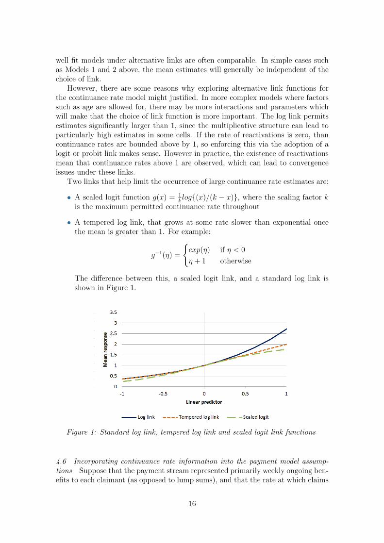
Two links that help limit the occurrence of large continuance rate estimates are:

• A scaled logit function g(x) = 1klog{(x)/(k − x)}, where the scaling factor k

is the maximum permitted continuance rate throughout

• A tempered log link, that grows at some rate slower than exponential oncethe mean is greater than 1. For example:

g−1(η) =

{exp(η) if η < 0

η + 1 otherwise

The difference between this, a scaled logit link, and a standard log link isshown in Figure 1.

Figure 1: Standard log link, tempered log link and scaled logit link functions

4.6 Incorporating continuance rate information into the payment model assump-tions Suppose that the payment stream represented primarily weekly ongoing ben-efits to each claimant (as opposed to lump sums), and that the rate at which claims

16

deactivate within each time period is roughly uniform. Then the results of the con-tinuance rate estimation should hold information relevant to the payments model.If Pij is the average amount paid to a claimant who continues to be active into thenext development period, then Pij would be expected to be equal to Pij for thosethat continue, and Pij/2 for those who deactivate. So:

Pij ≈ Pij

{cij +

1

2(1− cij)

}= Pij

(1

2+cij2

)The observed factors log(1

2+cij/2) can be used as offsets to the payments model,

resulting in easier estimation of the Pij, since the variability due to discontinuancehas been removed.

A similar approach can be used in traditional (non-GLM) contexts by scalingaverage payments

P ′ij = Pij

(1

2+ cij2

)before fitting the triangle. The adjustment helps to standardise the payment data;it corrects for unusually high or low deactivations before modelling.

4.7 Enforcing plausible continuance rates One area where GLM based approachesstill lag behind traditional approaches is the ability to easily modify selected contin-uance rate (or payment level) assumptions. This typically arises when the analystjudges there are factors affecting future continuance rates not reflected in the his-torical data. While ad hoc judgements are usually less desirable than historicalevidence, there are circumstances where they are unavoidable. For example, con-tinuance rates can be affected by changes in legistlation or claims managementpractices.

We propose two options to address the issue. First, the GLM can be imple-mented in a spreadsheet, so that a subsequent ad hoc selection can be easily applied.This implementation can be genuine (software such as Microsoft Excel has robustsolver routines that allow maximum likelihood optimizations to be performed), orvia GLM output from statistical software directly linking into a spreadsheet.

Second, there are ways to factor in judgements into the GLM itself. One of themore direct means is to “penalise” the likelihood function from departing signifi-cantly from prior beliefs that the analyst may impose. This can be interpreted in aBayesian or mixed model sense (see for example McCulloch and Neuhaus, 2001 orWest et al, 2007), or a frequentist approach to variance reduction (see the penalisedregression literature such as Tibshirani 1996, or Chapters 3 and 4 or Hastie et al2009). Suppose that L(N, c) is the likelihood function that depends on (amongother things) the observed numbers N = {nij} and the vector of continuance ratesfor the latest diagonals c = {c1, . . . cJ}. Suppose further that c∗ = {c∗1, . . . , c∗J} is aset of pre-determined continuance rate assumptions that the analyst prefers. Thenminimising the penalised expression:

−L(N, c) +J∑

j=1

λj(cj − c∗j)2

17

with penalty factors λj ≥ 0 will tend to push continuance factors towards the c∗.This approach is attractive because the integrated penalisation allows the statisticaladvantages of the GLM to be retained while giving some flexibility as the theadopted factors. The λj can be varied to influence how heavily selections shouldbe weighted towards the pre-judged estimates - as the λj get very large, the fittedcj will approach the c∗j . However there are challenges to this approach; statisticalsoftware has been slow to recognise the potential of penalised regression, and goodstarting choices of λj are not always available.

A similar approach can be used for payment models to impose competing beliefson adopted projection levels.

5 Concluding comments

We believe that there are significant advantages to using a GLM approach to reserv-ing problems such as PPAC models. While there is a cost in terms of complexityand ad hoc flexibility, these are increasingly minor as we discover the correct waysto setup models, and as the supporting software evolves. This paper addresses ahost of the pactical issues that allow an analyst to avoid a few of the pitfalls ofGLMs, further enabling their adoption.

Acknowledgements

This research has been supported by a grant from the Institute of Actuaries Aus-tralia, which I acknowledge with thanks.

References

Clark, D.R., & Thayer, C.A. (2004). A primer on the exponential family ofdistributions. Casualty Actuarial Society Spring Forum 117–148.

Dobson, A.J. (2002). An introduction to generalized linear models. CRC PressLLC.

England, P.D., & Verrall, R.J. (1999). Analytic and bootstrap estimates of pre-diction errors in claims reserving. Insurance: mathematics and economics, 25(3),281-293

England, P.D., & Verrall, R.J. (2002). Stochastic claims reserving in generalinsurance. British Actuarial Journal, 8(03), 443–518.

Fahrmeier, L. & Tutz, G. (1994). Multivariate statistical modelling based ongeneralized linear models. Springer.

Hastie, T., Tibshirani, R. & Friedman, J. (2009). sl The elements of statisticallearning (Vol. 2, No. 1). New York: Springer.

Mack, T. (1993). Distribution-free calculation of the standard error of chainladder reserve estimates. Astin bulletin, 23(02), 213–225.

McCullagh, P. & Nelder, J.A. (1989). Generalized Linear Models. London:Chapman and Hall.

McCulloch, C.E. & Neuhaus, J.M. (2001). Generalized linear mixed models.John Wiley & Sons, Ltd.

18

Taylor, G.C. (1986). Claims reserving in non-life insurance (Vol. 1). ElsevierScience Ltd.

Taylor, G.C. (2000). Loss reserving: an actuarial perspective. Boston: KluwerAcademic.

Tibshirani, R. (1996). Regression shrinkage and selection via the lasso. Journalof the Royal Statistical Society. Series B (Methodological), 267–288.

West, B.T., Welch, K.B., and Galecki, A.T. (2006). Linear mixed models:a practical guide using statistical software. CRC Press.

19

6 Appendix: Technical details

6.1 Theoretical results This section contains theoretical results supporting thearguments and claims made in the main body of the paper.

We adopt the same formulation for GLMs as Chapter 6 of Taylor (2000). Inparticular, the response Yij (either the continuance cij or payment level Pij) has thedistribution arising from an exponential family:

p(y) = exp

{yijθij − b(θij)

aij(φ)+ c(yij, φ)

}(6.1)

with aij(φ) = φ/wij and the mean equal to b′(θij) = g−1(XTβ).We define a GLM as disjoint if every predictor vector X ij related to cell (i, j)

comprises of a single 1 and otherwise zeros. Models 1, 2 and 3 in the paper all fit thisdefinition. The definition could be broadened to those that can be reformulated asdisjoint using a series of variable transformations and linear combinations. The firstresult is a relatively straightforward property of GLMs, included for completeness.

Result 1. If a GLM formulation is disjoint, then every parameter estimate is theweighted mean of those observations for which the corresponding variable is nonzero.

Proof. The disjoint formulation means that the maximum likelihood estimationcan be treated as a series of independent estimations on each of the groups ofobservations corresponding to each variable. That is, ifHm is the set of observationswhere the mth term of X ij is 1, then the parameter corresponding to X ij can beviewed as a maximum likelihood estimation of a intercept only model on Hm. Thusit is sufficient to prove that for an intercept model (where θij = θ a constant), theestimate recovered is the weighted mean.

Using (6.1), we see that the log-likelihood is

L =∑i,j∈H

φ−1wij{yijθij − b(θij)}+ c(yij, φ)

Setting θij = θ, differentiating by θ and setting to zero to maximise the log-likelihood,

0 =∑i,j∈H

φ−1wij{yij − b′(θij)} (6.2)

and so

g−1(XTβ) = b′(θij) =

∑wijyij∑wij

.

If g−1(XTβ) is the intercept model so the GLM estimate is a constant g−1(XTβ) =g−1(β), then this shows it must be the overall weighted average as required.

Result 1 has useful implications for the paper - in particular it shows that thesimple formulations of Models 1, 2 and 3 lead to parameters that recover the volumeweighted averages as claimed. This establishes the equivalence to traditional PPACmodel fits.

Result 2 demonstrates the increased volatility of running a deactivation/reactivationmodel compared to a single net deactivation model. But first we define:

20

• oij is the number of inactive claims in cell (i, j).

• For the deactivation/reactivation model, let dj be the (gross) continuance rate(applied to ni,j−1) and rj the reactivation rate (applied to oi,j−1).

We use capitalised versions (such as N ij for nij) to denote random variables forcell (i, j). We assume a standard chain ladder setup where cj if fixed for eachdevelopment year and estimates of cj are the volume weighted averages over H.

Result 2. Suppose that dj > 0.5 and that standard chain ladder estimates apply andare made for cj, dj and rj. Then the variance of one development period projectionvar(N ij|Ni,j−1, Oi,j−1) is lower for the net continuance rate model, compared to thedeactivation/reactivation model.

Proof. For the net deactivation model the number of actives in cell (i, j), N ij,depends on ni,j−1 and the estimate of cj, which can be regarded as a binomialvariable with ni,j−1 counts and mean cj which is estimated on K ..=

∑i:i,j∈H ni,j−1

observations.

var(N ij|Ni,j−1) = var(ni,j−1Cj)

= n2i,j−1

cj(1− cj)K

Now the net continuance rate is actually a combination of the deactivation andreactivation rates,

cj = dj +oi,j−1ni,j−1

rj .

Thus

var(N ij|Ni,j−1) = n2i,j−1

(dj +oi,j−1

ni,j−1rj)(1− dj − oi,j−1

ni,j−1rj)

K

=n2i,j−1dj(1− dj)

K+ni,j−1oi,j−1rj(1− 2dj)

K−o2i,j−1r

2j

K

<n2i,j−1dj(1− dj)

K, (6.3)

where the last uses the dj > 0.5 condition.For the deactivation/reactivation model, if we similarly define L ..=

∑i:i,j∈H oi,j−1,

var(N ij|Ni,j−1, Oi,j−1) = var(ni,j−1Dj + oi,j−1Rj)

= n2i,j−1

dj(1− dj)K

+ o2i,j−1rj(1− rj)

L(6.4)

Comparing (6.3) and (6.4) gives the desired inequality.

Three comments on Result 2:

21

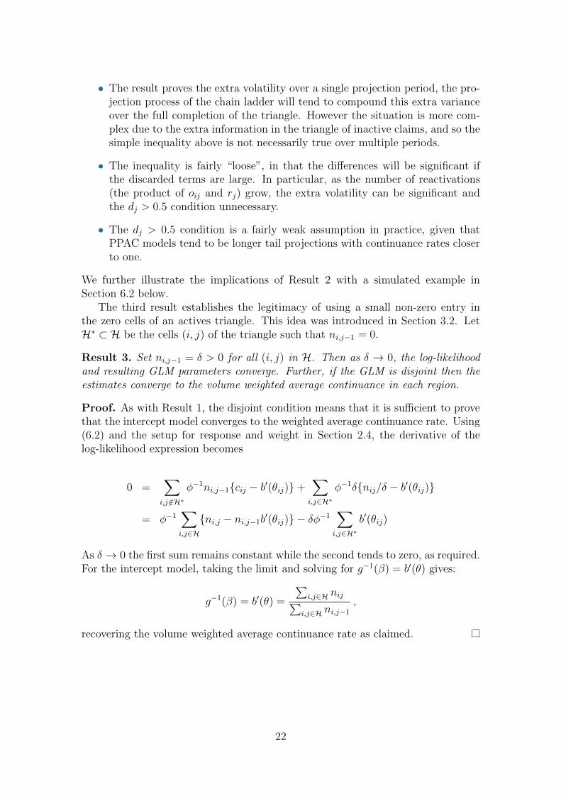
• The result proves the extra volatility over a single projection period, the pro-jection process of the chain ladder will tend to compound this extra varianceover the full completion of the triangle. However the situation is more com-plex due to the extra information in the triangle of inactive claims, and so thesimple inequality above is not necessarily true over multiple periods.

• The inequality is fairly “loose”, in that the differences will be significant ifthe discarded terms are large. In particular, as the number of reactivations(the product of oij and rj) grow, the extra volatility can be significant andthe dj > 0.5 condition unnecessary.

• The dj > 0.5 condition is a fairly weak assumption in practice, given thatPPAC models tend to be longer tail projections with continuance rates closerto one.

We further illustrate the implications of Result 2 with a simulated example inSection 6.2 below.

The third result establishes the legitimacy of using a small non-zero entry inthe zero cells of an actives triangle. This idea was introduced in Section 3.2. LetH∗ ⊂ H be the cells (i, j) of the triangle such that ni,j−1 = 0.

Result 3. Set ni,j−1 = δ > 0 for all (i, j) in H. Then as δ → 0, the log-likelihoodand resulting GLM parameters converge. Further, if the GLM is disjoint then theestimates converge to the volume weighted average continuance in each region.

Proof. As with Result 1, the disjoint condition means that it is sufficient to provethat the intercept model converges to the weighted average continuance rate. Using(6.2) and the setup for response and weight in Section 2.4, the derivative of thelog-likelihood expression becomes

0 =∑

i,j /∈H∗

φ−1ni,j−1{cij − b′(θij)}+∑

i,j∈H∗

φ−1δ{nij/δ − b′(θij)}

= φ−1∑i,j∈H

{ni,j − ni,j−1b′(θij)} − δφ−1

∑i,j∈H∗

b′(θij)

As δ → 0 the first sum remains constant while the second tends to zero, as required.For the intercept model, taking the limit and solving for g−1(β) = b′(θ) gives:

g−1(β) = b′(θ) =

∑i,j∈H nij∑

i,j∈H ni,j−1,

recovering the volume weighted average continuance rate as claimed.

22

6.2 Simulation results To further illustrate Result 2, we have constructed a sim-ple chain ladder problem for an active claim triangle:

• The triangle has 10 development years, plus a year 0.

• At year 0 in each row there are 100 claims active and 100 claims inactive

• (Gross) Continuance rates of 85% and reactivation rates of 1% are assumedin all development years.

We calculate the standard chain ladder estimates and complete the triangle, us-ing both a net continuance rate model and a deactivation-reactivation model, asdiscussed in Section 3.1. Our metric of interest is the standard deviation of thesum of the final (eleventh) row of the triangle,

∑10j=1 n11,j. This will be roughly

proportional to the liability for the most recent accident year, so is a good proxyfor understanding modelling volatility.

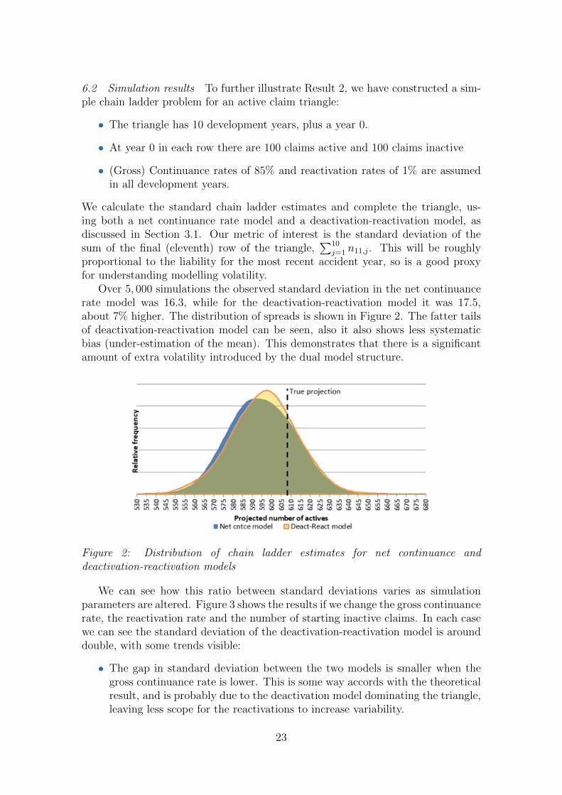
Over 5, 000 simulations the observed standard deviation in the net continuancerate model was 16.3, while for the deactivation-reactivation model it was 17.5,about 7% higher. The distribution of spreads is shown in Figure 2. The fatter tailsof deactivation-reactivation model can be seen, also it also shows less systematicbias (under-estimation of the mean). This demonstrates that there is a significantamount of extra volatility introduced by the dual model structure.

Figure 2: Distribution of chain ladder estimates for net continuance anddeactivation-reactivation models

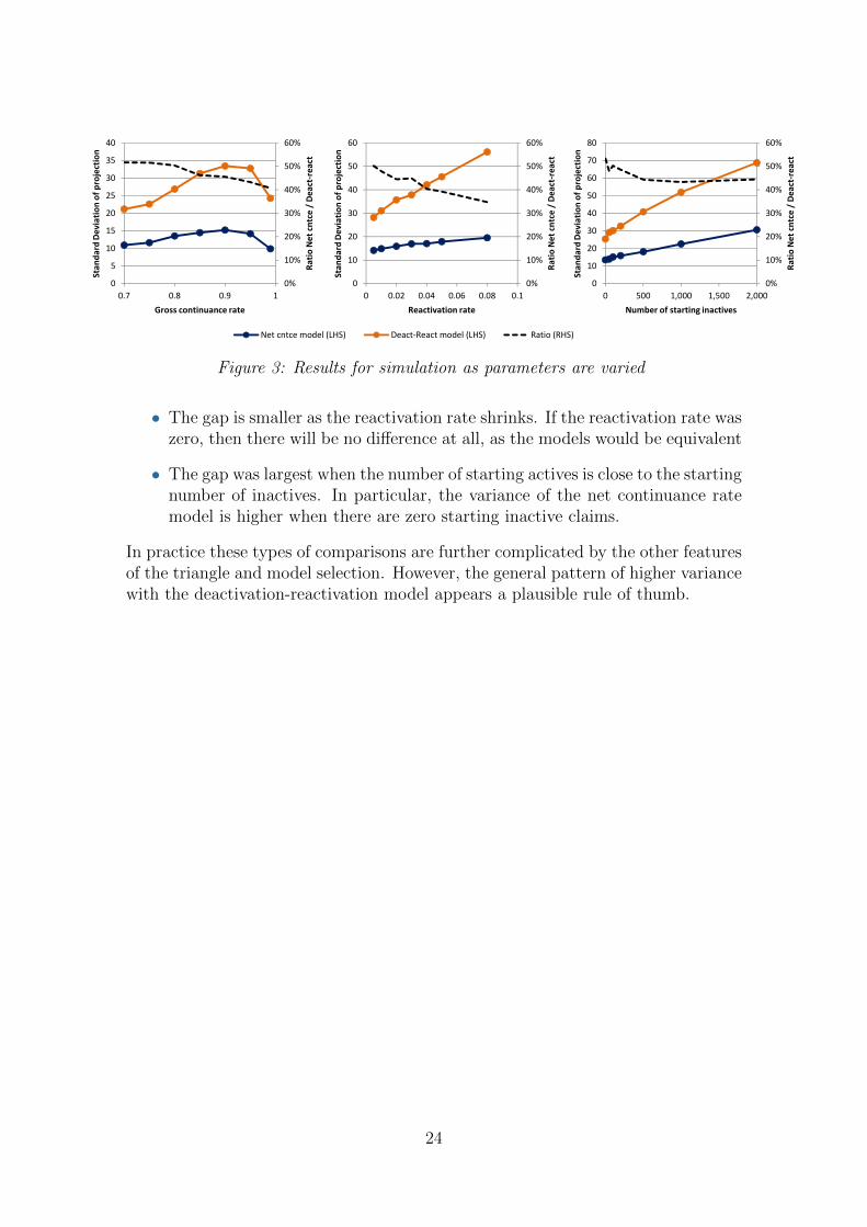
We can see how this ratio between standard deviations varies as simulationparameters are altered. Figure 3 shows the results if we change the gross continuancerate, the reactivation rate and the number of starting inactive claims. In each casewe can see the standard deviation of the deactivation-reactivation model is arounddouble, with some trends visible:

• The gap in standard deviation between the two models is smaller when thegross continuance rate is lower. This is some way accords with the theoreticalresult, and is probably due to the deactivation model dominating the triangle,leaving less scope for the reactivations to increase variability.

23

0%

10%

20%

30%

40%

50%

60%

0

5

10

15

20

25

30

35

40

0.7 0.75 0.8 0.85 0.9 0.95 1

Ra

tio

Ne

t cn

tce

/ D

ea

ct-r

ea

ct

Sta

nd

ard

De

via

tio

n o

f p

roje

ctio

n

Gross continuance rate

Net cntce model (LHS) Deact-React model (LHS) Ratio (RHS)

0%

10%

20%

30%

40%

50%

60%

0

5

10

15

20

25

30

35

40

0.7 0.8 0.9 1

Ra

tio

Ne

t cn

tce

/ D

ea

ct-r

ea

ct

Sta

nd

ard

De

via

tio

n o

f p

roje

ctio

n

Gross continuance rate

0%

10%

20%

30%

40%

50%

60%

0

10

20

30

40

50

60

0 0.02 0.04 0.06 0.08 0.1

Ra

tio

Ne

t cn

tce

/ D

ea

ct-r

ea

ct

Sta

nd

ard

De

via

tio

n o

f p

roje

ctio

n

Reactivation rate

0%

10%

20%

30%

40%

50%

60%

0

10

20

30

40

50

60

70

80

0 500 1,000 1,500 2,000

Ra

tio

Ne

t cn

tce

/ D

ea

ct-r

ea

ct

Sta

nd

ard

De

via

tio

n o

f p

roje

ctio

n

Number of starting inactives

Figure 3: Results for simulation as parameters are varied

• The gap is smaller as the reactivation rate shrinks. If the reactivation rate waszero, then there will be no difference at all, as the models would be equivalent

• The gap was largest when the number of starting actives is close to the startingnumber of inactives. In particular, the variance of the net continuance ratemodel is higher when there are zero starting inactive claims.

In practice these types of comparisons are further complicated by the other featuresof the triangle and model selection. However, the general pattern of higher variancewith the deactivation-reactivation model appears a plausible rule of thumb.

24