bryan e howard. evaluation of text classification accuracy
TRANSCRIPT

Bryan E Howard. Evaluation of Text Classification Accuracy. A Master’s Paper for the M.S. in I.S. degree. November, 2007. 50 pages. Advisor: Catherine Blake
Libraries such as the National Library of Medicine frequently assign terms from a
controlled vocabulary to improve document retrieval. The high cost of such manual
efforts has motivated work in automated document classification. Framed using the
knowledge discovery process, this paper compares classification performance based on
various preprocessing, transformation and data mining methods. Specifically, we explore
the degree to which stemming, vocabulary selection using term weighting, and
windowing increases classification accuracy of the Naïve Bayes and J48 algorithms. We
find that a process using the Naïve Bayes algorithm with a stop list, removal of data
anomalies, TF*IDF weights in the range of 15 to 20, and a three word window size will
provide the highest classification accuracy.
Headings:
Text Mining
Data Mining
Knowledge Discovery in Databases
Naïve Bayes
J48

EVALUATION OF TEXT CLASSIFICATION ACCURACY
by Bryan E Howard
A Master’s paper submitted to the faculty of the School of Information and Library Science of the University of North Carolina at Chapel Hill
in partial fulfillment of the requirements for the degree of Master of Science in
Information Science.
Chapel Hill, North Carolina
November 2007
Approved by
_______________________________________
Catherine Blake

1
Table of Contents 1 Introduction................................................................................................................. 2 2 KDD Overview ........................................................................................................... 4 3 Literature Review........................................................................................................ 6 4 Methodology............................................................................................................... 9 4.1 Selection.................................................................................................................. 9 4.2 Preprocessing ........................................................................................................ 13 4.3 Transformation...................................................................................................... 16 4.3.1 Stemming .......................................................................................................... 16 4.3.2 Term Weight ..................................................................................................... 17 4.3.3 Window Size..................................................................................................... 18 4.4 Data Mining .......................................................................................................... 19 5 Results and Analysis ................................................................................................. 20 5.1 Stemming Analysis ............................................................................................... 23 5.2 Term Weight Analysis .......................................................................................... 25 5.4 Algorithm Analysis............................................................................................... 30 5.5 Vocabulary Analysis............................................................................................. 32 6 Conclusion ................................................................................................................ 35 7 References................................................................................................................. 37 Appendix A: Journals Used in Selection Criteria ............................................................. 40 Appendix B: Special Characters Replaced ....................................................................... 47 Appendix C: Contents of Anomaly File ........................................................................... 48

2
1 Introduction
People are creating and recording more information now than any time in history.
With the introduction and proliferation of computers, much of this information is being
stored for later use. The large volume of data available has created many issues including
how to find a document or a group of documents. When someone runs a search, they
specify criteria to select relevant documents. Classifying the documents in some manner
increases the searcher’s chance of retrieving a relevant group of documents. The
classification of documents introduces issues as well, including how to accurately classify
documents. Some organizations have highly trained employees to classify their
documents, such as the National Library of Medicine. However, the high cost of manual
classification provides a strong motivator towards developing accurate automatic
classification.
Text mining is one solution, which can classify text documents into a predefined
set of categories automatically. Mining textual information is a multi-step process. The
steps are: selection, preprocessing, transformation, data mining, and
interpretation/evaluation [6]. Variations of each step are possible, including removing
meaningless words in preprocessing, reducing words down to their root in
transformation, and using different classification algorithms in data mining. With all the
variations possible there is a question of what process works best for

3
text mining. The information available on various text mining procedures makes it
difficult for organizations to choose a method that best meets their needs.
This paper evaluates some of the steps of the text mining process to determine
what variations result in higher classification accuracy of the corpus of documents. We
ran tests in the transformation and data mining steps of the process and analyzed the
results. The specific tests evaluated how stemming, word phrases, term weighting, and
different algorithms affected the classification accuracy. The results indicate which
transformation methods and data mining algorithms give the highest level of
classification accuracy. The results also show what methods do not help the
classification accuracy. Removal of the useless methods will reduce the processing time
and effort of the text mining process.
Section two of this paper will introduce the steps of the KDD (Knowledge
Discovery in Databases) process with a brief over view of some of the methods. The
literature review section covers some of the background of data and text mining. The
methods section will cover the how the steps in KDD were accomplished and any issues
that arose during the steps. The results and analysis section will discuss the findings of
the tests. The conclusion section will provide the recommendations based on the results
of the testing.

4
2 KDD Overview
Figure 2.1. An Overview of the Steps that Compose the KDD Process. Source: Fayyad, U., Piatetsky-Shapiro, G., Smyth, P. “From Data Mining to Knowledge Discovery in Databases.” IA Magazine 17.3 (1996): 37-54.
The KDD process is composed of the following steps: 1) selection, 2)
preprocessing, 3) transformation, 4) data mining, and 5) interpretation and evaluation (see
Figure 2.1). The selection step creates the target data, a subset of the available data. The
remaining steps in the KDD process use the target data, not all the available data. The
criteria for creating the subset can be most anything, such as article topics, corresponding
data sources, date range, etc. The data is “cleaned” in the preprocessing step. The
cleaning can include deciding how to handle missing data, removal of useless text, and
handling of special characters. The use of a stop list to remove common words is an
example of a method of preprocessing. The reduction of the amount of data by some
method happens in the transformation step. Stemming, the reduction of a word to its root

5
form, and term weighting, the assigning of a weight to a word by its frequency, are two
common methods of transformation. Determining the appropriate algorithms and
processing the data through the algorithms is included in the data mining step. The data is
reviewed, analyzed, and possibly used to discover new information in the final step of
interpretation and evaluation. [6, 7]
6
3 Literature Review
Researchers have posed a variety of algorithms for text classification purposes
[1,9,11,12,15,18,20,22,23]. These comparisons focus mainly on new algorithms and how
they perform compared to other algorithms. This is useful information, but the algorithm
is only one step of the overall KDD process. Evaluating the importance of the other steps
is also essential to discovering a process that is highly accurate and efficient.
Two frequently used algorithms are Naïve Bayes[2] and the C4.5 algorithm[14].
The Naïve Bayes algorithm is a commonly utilized algorithm in text classification
[15,22]. Some researcher report that Naïve Bayes performs poorly [22] for text
classification, but others report good performance [12,22]. One issue with this algorithm
is that it is reported to be “sensitive to term space reduction” which causes classification
to suffer [23]. Joachims has shown that the Naïve Bayes algorithm will out perform other
algorithms, including the C4.5 algorithm, in some situations, but not others [9].
Many researchers have evaluated decision tree algorithms, including C4.5, in
regard to text classification. The idea behind this type of algorithm is to build a tree of
questions that will help decide an outcome. Research has shown that the C4.5 algorithm
can out perform other algorithms in text classification, including the Naïve Bayes
algorithm, depending on the situation [9].
Some text mining methods that are not as frequently tested include the use of
stemming, term weighting, and word phrases. Variations of these methods also have the
potential to affect the accuracy of text classification, just as the use of different

7
algorithms. As an example, Blake and Pratt found that “increasing the semantic richness
of features” increased the usefulness of association rules [3].
The use of a stop list to remove common, but meaningless words is a standard
approach to reducing the dimensionality of data. Examples of these meaningless words
include “a” and “the”. Both of these words are frequently in a document, but are not
meaningful to the document context. The words in the corpus that match any word in the
stop list are removed from the data. The practice of using a stop list is common and not
normally considered for testing in the text mining process [1,3,11,17,20].
Stemming, a transformation method, converts words to their root form.
Stemming reduces the number of unique words in a document by combining all forms of
a word into one root form. The reduction in unique words can affect the results of the
overall process. For example, if document A only uses one form of a word and document
B only uses a second form of the word, changing both words to their root form could
change the results. Since the root form of the word is associated with both types of
documents it is not a definitive indicator of the document type. Stemming is discussed in
some of the text mining literature but the results are inconclusive. Most studies report
that the use of stemming will help categorization in some situations, but hurts it in other
situations [4,8,10,17]. Dave, Lawrence, and Pennock noted that when the Porter stemmer
was used the performance of the classifier was higher than the baseline in one test but
lower in the second [4]. In Harmon’s test of three stemming algorithms, including the
Porter Stemmer, her results showed the use of stemming “did not result in improvements
in retrieval performance...as measured by classical evaluation techniques” [8]. Harmon
also stated there were instances where the performance was improved, but the number of

8
instances with poorer performance was about the same. These results lead to the overall
conclusion that stemming did not improve performance [8].
Another method of transformation often used to reduce the dimensionality of data
in text mining is term weighting [4,15,21]. Two commonly used term weighting
algorithms are term frequency and document frequency. A term’s weight, calculated by
how frequently it occurs in a single document or all documents, can eliminate the term
from inclusion in a data set. Yang and Pedersen suggest eliminating terms that rarely
occur in all documents may help performance if they are irrelevant terms [21]. Work by
Rogati and Yang shows that removal of rare words in all documents increases the
performance of text categorization [15]. Their work also concluded that weighting by
term frequency performs poorly compared to other weighting methods [15].
Another method to reduce dimensionality in text mining is the use of word
phrases. The word phrases are composed of meaningful words adjacent to each other in
the text. Window size is the number of words contained in the phrase. The idea behind
this method is that phrases may improve text mining of documents compared to the
evaluation of individual words [10].

9
4 Methodology
Our goal in this project, is to test the classification accuracy of articles with
similar and dissimilar topics. We hypothesized that text mining would have the highest
classification accuracy when comparing dissimilar topics. As the similarity of the classes
increased, we anticipated the classification accuracy would decrease. As a control, we
also wanted to compare against a corpus of data that did not include the other topics.
We also wanted to test how some of the more common preprocessing and transformation
methods affected classification accuracy. We chose to test some of the methods that did
not intuitively seem useful in the process. Removing meaningless words, i.e. using a stop
list, is a logical step from a human point of view. When we analyze a document for it’s
topic we do not consider the words “a”, “the”, “as”, “an”, etc. in the analysis. These
words are part of the language structure and do not convey meaning. The methods we
test include stemming, word phrases, and term weighting.
4.1 Selection
To begin the text mining process we needed to identify a data source of text
documents from which we could build the target data. The data source needed to have
pre-categorized documents so we could validate the classification accuracy. We also
wanted the retrieval of documents from the data source to be relatively easy. With these
goals in mind we decided to use documents from PubMed, a National Library of

10
Medicine website. It meets all the goals plus we were able to use the ESearch utility
provided by the NLM in our selection process.
Another goal of the project was to run tests against a large data set. After some
thought we decided to call a large data set a group of 2,000 or more articles. We thought
this number of articles would result in a large number of words per corpus. When we
created the first two corpora there were 2,358 articles in each. After processing the text
we ended up with 220,975 words for the first topic, also referred to as the class, and
293,200 words for the second class.
Before we ran all the data through the text mining process we did initial tests with
the first two corpora. At the end of the initial test we discovered that the implementation
of one of the algorithms in the text mining tool could not handle the number of terms.
We started reducing the number of articles in each corpus until the algorithm could
handle most of the tests. Each corpus ended up containing 500 articles. This reduced the
number of words for the first corpus to 55,532 and the second to 61,610. We checked
the third and fourth corpus at a later time and the third had 65,805 words and the fourth
corpus had 61,967 words.
As discussed in the introduction to section 4, we wanted to test one topic against a
similar topic, a dissimilar topic, and a control topic. Since PubMed is a medical data
store we picked lung cancer as the main topic to compare against the others. We then
picked breast cancer as our similar topic since both are types of cancer. We picked
hypertension as the dissimilar topic, since it and cancer are not related medical
conditions. The control corpus, which we refer to as the NULL corpus, contains any
articles not classified as lung cancer, breast cancer, or hypertension by PubMed.

11
The National Library of Medicine uses a controlled vocabulary to classify article
subjects, referred to as MeSH (Medical Subject Headings). In the selection criteria used
for lung cancer, breast cancer, and hypertension they had to be classified as a major
MeSH topic to be included. The NULL corpora search criteria excluded any articles
where the MeSH classification included lung cancer, breast cancer, or hypertension.
When the NULL corpus was built we noticed there were a few hypertension related
articles in the corpus. We manually removed these articles from the corpus before any
further processing.
Another of our selection criteria was to retrieve documents from highly relevant
medical journals. We created a list of relevant journals by searching the ISI Web of
Knowledge 2005 Journal Summary List. The subject categories we used were medicine:
general and internal and medicine: research and experimental. We included the first
eighty journals from the category medicine: general and internal, ordered by impact
factor, in the selection criteria (see Appendix A). The first sixty journals from the
category medicine: research and experimental, order by impact factor, were added to the
selection criteria (see Appendix A). If the journal’s title included the word cancer,
hypertension, or a synonym of either we excluded it from the final list. While evaluating
the ESearch utility using the journal list, we discovered that Pubmed was not using the
ISSN number for the British Medical Journal that the journal citation report had listed.
Instead, Pubmed uses three different ISSN numbers for the British Medical Journal,
0267-0623, 0007-1447, and 0959-8138. We added these ISSN numbers to the article
search criteria. When we started the evaluation of the ESearch utility we had a list of
approximately 40 journals, all from the medicine: general and internal category. Using

12
only these 40 journals, we were unable to retrieve an acceptable number of articles. After
several iterations of adding journals and checking the number of retrieved articles we
found that the 140 journals detailed above gave a sufficient number of articles.
Another of the selection criteria we used was setting a date range for the retrieved
articles. When we began the project we were using a range of January 1st, 1991 to
December 31st, 2006. The number of articles returned for the hypertension and NULL
topics were not large enough with this date range. After testing various date ranges with
all four topics we found that it was going to be impossible to get approximately the same
number of articles with the same date range. We decided to use a date range that
gathered more articles than needed for all four topics and a limit was added to the java
program that creates the corpora. The date range settled on was from January 1st, 1900 to
March 18th, 2007.
To create the four corpora in an automated fashion we wrote a Java program to
create text files that could be further processed. The program, called pulldata has six
inputs: 1) maximum number of articles to return, 2) NLM database to search, 3) input file
containing journals and subject to search, 4) beginning date, 5) end date, and 6) output
file name. The program uses the ESearch and EFetch utilities provided by the NLM in
finding and retrieving the articles. The program first uses the selection criteria entered
from the command line and input file to get a list of article IDs via the ESearch utility.
Once the list of articles is built the program loops through each article ID retrieving the
data via the EFetch utility. The data, in XML format, is then written to the output file
designated in the command line.

13
4.2 Preprocessing
To simplify the rest of the text mining processing we decided to put the
information in a database. We created a table that would hold the article id (also referred
to as PMID), sentence number, word number, topic (also referred to as class name),
word, document frequency, term frequency, and TF*IDF (see Figure 4.1). The last three
fields relate to the transformation step. We added a primary key across the columns
pmid, sent_num, word_num, and class_name to make sure duplicate data was not loaded
into the table. We created a program named preformat to perform the preprocessing tasks
including splitting each abstract into sentences and then words, removal of special
characters, removal of anomalies, evaluation of words against a stop list, and inserting the
remaining words into a table. The pmid, sentence number, word number, and class name
associated with the word, i.e. the metadata for the word, are also inserted into the table.
The preformat program has six inputs: 1) the input data file, 2) the stop word list to use,
3) the table to insert data into, 4) the data class name, 5) log file for the program, and 6)
the anomaly file to use.
PRJ110_LH_SM
PK PMIDPK SENT_NUMPK WORD_NUMPK CLASS_NAME
WORDDFTFTF_L_IDF
Figure 4.1

14
The first task of the preformat program is to open the input file containing the
XML formatted data and read through each article ID. If the article does not have an
abstract it moves to the next article. If the article has an abstract the program loads the
abstract into memory so it can finish the preprocessing before inserting the data into the
table. The abstract is then broken down into sentences by searching for the pattern of a
period, exclamation point, or question mark followed by a single space. As this pattern is
found, the sentence is numbered and placed into memory.
Once all the sentences have been identified the program loops through each
sentence. The program evaluates each sentence, character by character, looking for
special characters. If special characters are found they get replaced with a single space
(see Appendix B). During testing these special characters caused issues with loading of
data, sentence counts, and word counts. After reviewing the issues we decided the
special characters were of no value in classification, so they were replaced with a space
during subsequent testing. During the testing we did try removing the special characters,
but this created invalid words in some cases. For example, the word “P<.001)” became
“P001” instead of the words “P” and “001”.
The next task of the program is to create a list of individual words in the sentence.
To do this the program splits the sentence at each space and then converts individual
words to lower case. Next, the program removes left over punctuation at the end of each
word, such as a period, exclamation point, or question mark. This step is necessary
because the last word of each sentence will still have the punctuation appended.
Using an iterative process, we manually inspected the words to identify terms we
call anomalies from the end of a word (see Appendix C). All the anomalies we

15
encountered in the corpora are units of measurement, such as “-hrs” or “-kg”. We also
removed the characters “-” and “--” from the beginning of the word.
The program then checks the word to see if it contains a hyphen. The program
splits words containing a hyphen into two, and then checks if the subsequent parts are
numbers. Numerical terms are changed to null, otherwise the word is left unchanged.
This step is necessary to remove mathematical formulas encountered in the data, such as
69-1. In our preliminary tests, most of the formulas encountered were unique and cause
issues with classification. We then evaluate the word to make sure it has a length greater
than zero and is not numerical. Checking the length of the word is necessary due to the
previous step where the program introduces nulls into the data. Numerical values, which
were frequent in all corpora, do not help in classification and are thus removed.
Next, the program compares each word against a modified stop list. After we
obtained the original stop list [16] we found through testing that more words needed to be
added to the list. During our tests we found words that were meaningless to classification
and could be removed. Most of the words are related to dates, quantities, or numbers not
expressed as Arabic symbols. We added these meaningless words to our stop list. We
found a few instances where previous preprocessing steps reduced a word down to a
single character. To eliminate this problem we added all the letters of the alphabet to the
stop list.
The final step in our preprocessing is to insert the word and it’s metadata into a
table. Since we are testing classification accuracy of three different groups of data, we
created three different tables to hold the data. The first table holds the lung cancer and
breast cancer data, the second has the lung cancer and hypertension data, and the final

16
table has the lung cancer and NULL data. To reduce preprocessing time we only loaded
the lung cancer data into one table and then copied it to the other tables.
4.3 Transformation
4.3.1 Stemming
In this project we wanted to test how the use of stemming, a transformation
method, effects classification accuracy. We also wanted to have both the stemmed and
non-stemmed data available and be able to use the same programs in the text mining
process. The simplest way to do this was to create three new tables to hold the stemmed
data with almost the same structure as the non-stemmed data. We added a column,
named pre_word, to these new tables. This column holds the original form of the word
and the word column holds the stemmed version (see figure 4.2). To apply stemming we
created a program named modstemmer. This program uses the Java implementation of
the Porter Stemmer obtained from [13]. The program has two inputs: 1) source table and
2) destination table. It is a “wrapper” program that reads data from the non-stemmed
table, applies stemming to the word, and then saves the stemmed word, original word,
and metadata in the destination table.
Figure 4.2

17
4.3.2 Term Weight
Another transformation method that we tested is how term weighting affects
classification accuracy. After looking at the different types of weighting we decided to
evaluated term frequency times inverse document frequency weighting, commonly
referred to as TF*IDF. To be able to calculate TF*IDF each word’s term frequency (TF)
and document frequency (DF) has to be calculated first. After the TF and DF values are
obtained the TF*IDF weight can be calculated. We used the formula: Wij = tfij *
log2(N/n) to calculate the TF*IDF value [5]. In the formula the N equals the number of
documents in the corpus and n equals the number of documents that contain the word at
least once.
We created another program, named tfidf, to calculate the term frequency,
document frequency, and TF*IDF of each word. The one input to the program is the
name of the table it runs the calculations against. The column names that contain the
weight calculations are tf, df, and tf_l_idf for term frequency, document frequency, and
TF*IDF respectively. The first step of the tfidf program is to calculate the term
frequency of each word. This calculation is made by creating a list of distinct words for
each document. It then computes the number of times each word occurs in the document
and updates the tf column with the count. The second step of the tfidf program is to
calculate the document frequency of each distinct word in the corpus. It creates a distinct
list of words in the table and then loops through each word counting the number of
documents that contain the word. When it is finished it updates the df column with
result. The last step of the program is to calculate the TF*IDF of each word. First the
program retrieves the number of distinct documents in the table (i.e. corpus). It then gets

18
the term frequency and document frequency of each, calculates the result of the Wij = tfij
* log2(N/n) algorithm, and updates the tf_l_idf column with the result.
4.3.3 Window Size
The last transformation method that we tested was how different term window
sizes affected classification accuracy. Term window size is the number of words that are
grouped together to be used as a single dimension. Each word is considered a dimension
if you have a window size of one. Each three word phrase in a sentence is considered a
dimension if the window size is set to three. We evaluated window sizes of one, three,
and five words in length. We created a program, named WindowOutput, to output the
contents of a table, in the file format of our data mining tool, with the appropriate
window size and TF*IDF value. The program has four inputs: 1) window size, 2)
TF*IDF threshold, 3) table to extract data from, and 4) output file name.
The first step of the WindowOutput program is to build the header of the output
file with comments detailing the window size, source table, and TF*IDF limit used. Next
the program outputs a line containing the possible attribute term values. The number of
term lines equals the window size. If the window size is three then there will be three
term definition lines. The possible values of each term are all the distinct words in the
table. Next the program outputs the attribute class definition. This is a list of all the
classes, i.e. topics, in the table. We build this list the by retrieving the distinct class
names in the table. For example, the table containing data about lung cancer and
hypertension will have the classes LC and HT, respectively. Next the program outputs
the data to be analyzed by the mining tool. Each line of data contains the number of
terms equal to the window size, separated by commas, and then the data’s class. For

19
example, if the first three words of a sentence in a lung cancer article are nursing,
intervention, and breathlessness then the line of data would be
“nursing,intervention,breathlessness,LC”. This example assumes the window size is set
to three.
4.4 Data Mining
In the data mining step we wanted to compare the classification accuracy of a
C4.5 and Naïve Bayes algorithm. The data mining tool we used in our tests was the Java
implementation of Weka [19], version 3.4.10. Weka includes the Naïve Bayes and J48
algorithms in its distribution. The J48 algorithm is a Java implementation of the C4.5
decision tree algorithm. When we ran the tests we did not specify a test file for Weka to
use. By leaving this out we caused Weka to perform ten-fold cross validation during the
tests. The results of each test provided the percent of documents correctly classified and
incorrectly classified. These percentages were used to create spreadsheets depicting the
results of the tests using the different methods and algorithms.

20
5 Results and Analysis
Chart 5.1
Lung Cancer & Breast Cancer Non-Stemmed Summary
55
60
65
70
75
80
85
90
95
100
>5 >6 >7 >8 >9 >10 >11 >12 >13 >14 >15 >16 >17 >18 >19 >20
TFIDF
% C
orre
ctly
Cla
ssifi
ed
J48 WS 1NB WS 1J48 WS 3NB WS 3J48 WS 5NB WS 5

21
Chart 5.2
Lung Cancer & Breast Cancer Stemmed Summary
55
60
65
70
75
80
85
90
95
100
>5 >6 >7 >8 >9 >10 >11 >12 >13 >14 >15 >16 >17 >18 >19 >20
TFIDF
% C
orre
ctly
Cla
ssifi
ed
J48 WS 1NB WS 1J48 WS 3NB WS 3J48 WS 5NB WS 5
Chart 5.3
Lung Cancer & Hypertension Non-Stemmed Summary
55
60
65
70
75
80
85
90
95
100
>5 >6 >7 >8 >9 >10 >11 >12 >13 >14 >15 >16 >17 >18 >19 >20
TFIDF
% C
orre
ctly
Cla
ssifi
ed
J48 WS 1NB WS 1J48 WS 3NB WS 3J48 WS 5NB WS 5

22
Chart 5.4
Lung Cancer & Hypertension Stemmed Summary
55
60
65
70
75
80
85
90
95
100
>5 >6 >7 >8 >9 >10 >11 >12 >13 >14 >15 >16 >17 >18 >19 >20
TFIDF
% C
orre
ctly
Cla
ssifi
ed
J48 WS 1NB WS 1J48 WS 3NB WS 3J48 WS 5NB WS 5
Chart 5.5
Lung Cancer & Null Set Non-Stemmed Summary
55
60
65
70
75
80
85
90
95
100
>5 >6 >7 >8 >9 >10 >11 >12 >13 >14 >15 >16 >17 >18 >19 >20
TFIDF
% C
orre
ctly
Cla
ssifi
ed
J48 WS 1NB WS 1J48 WS 3NB WS 3J48 WS 5NB WS 5

23
Chart 5.6
Lung Cancer & Null Set Stemmed Summary
55
60
65
70
75
80
85
90
95
100
>5 >6 >7 >8 >9 >10 >11 >12 >13 >14 >15 >16 >17 >18 >19 >20
TFIDF
% C
orre
ctly
Cla
ssifi
ed
J48 WS 1NB WS 1J48 WS 3NB WS 3J48 WS 5NB WS 5
5.1 Stemming Analysis
The results of testing stemming on the three corpora of data show there is little
difference in the percentage of correctly classified articles when the data is stemmed and
when it is not. Table 5.1a, an excerpt of table 5.1, shows the classification accuracy
percentages for the lung cancer and hypertension corpus when stemming is applied and
when it is not.
The second and third columns, labeled “NS NB WS 3” and “ST NB WS 3”, show
the classification results from the Naïve Bayes algorithm for the stemmed and non-
stemmed data with a window size of three. The fourth column shows the difference in
classification accuracy for the values in the second and third. The largest difference in

24
TFIDF NS NB WS 3†
ST NB WS 3† Diff Ŧ
NS J48 WS 5†
ST J48 WS 5† Diff Ŧ
NS NB WS 5†
ST NB WS 5† Diff Ŧ
>5 88.02 88.97 0.95 * 77.92 91.64 92.31 0.67>6 89.18 90.36 1.18 * 78.97 92.48 93.3 0.82>7 90.73 91.38 0.65 78.48 80.08 1.6 93.56 93.97 0.41>8 91.79 92.44 0.65 79.08 80.68 1.6 94.32 94.73 0.41>9 93.5 93.56 0.06 81.15 81.9 0.75 95.4 95.38 -0.02>10 95.19 95.2 0.01 85.25 85.45 0.2 96.62 96.62 0>11 95.64 95.5 -0.14 85.46 85.19 -0.27 96.58 96.49 -0.09>12 96.1 95.82 -0.28 85.63 85.37 -0.26 96.78 96.63 -0.15>13 96.42 95.98 -0.44 85.92 86.19 0.27 97.16 96.77 -0.39>14 96.52 96.28 -0.24 85.94 87.12 1.18 97.08 96.93 -0.15>15 96.79 96.44 -0.35 85.74 87.14 1.4 96.73 96.49 -0.24>16 96.92 96.82 -0.1 86.88 87.69 0.81 96.76 96.74 -0.02>17 97.07 96.96 -0.11 86.49 87.41 0.92 96.87 96.93 0.06>18 97.09 97.17 0.08 86.48 87.86 1.38 96.68 96.74 0.06>19 97.38 97.24 -0.14 86.25 87.84 1.59 96.9 96.91 0.01>20 97.47 97.55 0.08 88.59 89.53 0.94 96.76 96.83 0.07
Table 5.1a: Partial Classification Results of Lung Caner and Hypertension Corpus † Percent correctly classified. NS=Non-Stemmed; ST=Stemmed; NB=Naïve Bayes;
WS=Window Size. Ŧ Value is the difference in percent correctly classified between stemmed and non-
stemmed. A negative value indicates the non-stemmed classification percentage is higher.
* Data not available
the results is 1.18%, with 3/4ths of the values in the fourth column being within a half
percent of each other. For a TFIDF value greater than 16 the classification accuracy is
96.92% for the non-stemmed data and 96.82% for the stemmed data, which is .1%
difference in accuracy. Small differences in accuracy occur through out the results.
Another example of this is shown in the classification results for the J48 algorithm with a
window size of five and a TFIDF value greater than 10. The classification accuracy is
85.25% for the non-stemmed data and 85.45% for the stemmed data, a difference in
accuracy of .2 percent. When we analyze all the results the difference in classification
accuracy ranges from zero, indicating an exact match, to 2.06 percent. Of the 77 result
sets, 62 (80.5%) differ by less than 1 percent, 13 (16.9%) differ between 1 and 2 percent,

25
and 2 (2.6%) have a difference of 2.06 percent. Tables 5.1, 5.2, and 5.3 show the results
and differences in classification accuracy by algorithm, window size, TFIDF value, and if
the data was stemmed for all tests. In table 5.3, several values from the J48 algorithm for
the stemmed and non-stemmed data having a window size of five are erroneous due to
over fitting and too little data to create the decision matrix. The erroneous values and
their differences have a plus symbol beside them.
5.2 Term Weight Analysis
Analysis of the test results show that term weighting improves the classification
accuracy in most cases. Overall, the results show that the higher the TF*IDF value the
higher the percentage of the data that is correctly classified. Charts 5.1 through 5.6 plot
the results of the tests for all corpora of data and an upward trend is apparent in all but
two plot lines. The plot lines labeled J48 WS 5 in charts 5.5 and 5.6 do not show the
same upward trend as the others. The plot line in chart 5.6 starts with an upward trend
but at the TF*IDF value greater than 17 it falls to 60.5% from a previous value of 84.85
percent. The plot line in chart 5.5 is more erratic jumping from 55.81% to 77.62% at one
point in the graph. A few points down the graph it then jumps from 81.36% to 67.26
percent. These two plots show the classification accuracy of the J48 algorithm using
non-stemmed and stemmed data with a window size of five. We checked the output files
for these tests and they indicate the problems came from over fitting and too little data to
create the decision matrix.

26

27

28

29
A detailed review of the charts show some trends tied to term weight values and
algorithms type. In all the charts, if the Naïve Bayes algorithm is used and the window
size is not one there is a point where the increase in classification accuracy starts to level
out. For charts 5.3, 5.4, 5.5, and 5.6 this point is at the TF*IDF value of greater than 10.
The point where this occurs in charts 5.1 and 5.2 is at the TF*IDF value of greater than
12. Once this point is reached the classification accuracy may increase at a slower rate or
vary a small amount up and down as the term weight increases. The trend for the J48
plots and the Naïve Bayes plots having a window size of one is a steady increase in
classification accuracy as the term weight increases. There is not a discernable leveling
of in these plots. Another interesting artifact is that in charts 5.1 and 5.2 the results from
the Naïve Bayes algorithm for data with a window size of five hit a peak at the term
weight of greater than 17. This happened for the stemmed and non-stemmed data and
only for the lung cancer and breast cancer corpus. We are unsure of why this happened
but one possibility is that the similarity of the corpus made five word phrases with
weights higher than 17 less useful in the classification process.
5.3 Window Size Analysis
The results of the widow size tests show there is an increase in classification
accuracy as the window size is increased for the Naïve Bayes algorithm. The J48
algorithm reacts in an opposite manner. As the window size is increased the
classification accuracy of the J48 algorithm decreases. One result of interest is that when
the window size is one the classification accuracy of the J48 and Naïve Bayes algorithms
are the same in all charts. In charts 5.1 through 5.6 the results show that for the Naïve
Bayes algorithm when the window size is increased from one to three there is a

30
considerable increase in classification accuracy. This increase is not as apparent when
the window size is increased from three to five. In some of the results for the Naïve
Bayes algorithm, such as charts 4.1 and 4.4 the classification accuracy for window size
three will exceed that of window size 5 at the highest TF*IDF values. The J48 accuracy
results do not show such a considerable decrease when the window size changes from
one to three. The J48 results also show a decrease in accuracy proportional to the first
when the window size changes from three to five, unlike the Naïve Bayes results.
5.4 Algorithm Analysis
The results of testing all corpora of data with the Naïve Bayes and J48 algorithm
show that in all cases the Naïve Bayes algorithm performs no worse than the J48
algorithm. In all cases where the window size is greater than one the Naïve Bayes out
performs the J48 results. These results can be seen in charts 5.7, 5.8, and 5.9. One
problem we did discover is that the J48 algorithm can not handle as large an amount of
data as the Naïve Bayes algorithm. In all the charts you will see that there are missing
data points in the J48 plots at the lower term weights with a window size of one and
three. The J48 algorithm would run out of memory before it could finish. We set the
available memory as high as Java would let us via the “-Xmx” parameter, but it still was
not enough memory.

31
Chart 5.7
Lung Cancer & Breast Cancer Summary Chart
55
60
65
70
75
80
85
90
95
100
>5 >6 >7 >8 >9 >10 >11 >12 >13 >14 >15 >16 >17 >18 >19 >20
TFIDF
% C
orre
ctly
Cla
ssifi
ed
NS J48 WS 1ST J48 WS 1NS NB WS 1ST NB WS 1NS J48 WS 3ST J48 WS 3NS NB WS 3ST NB WS 3NS J48 WS 5ST J48 WS 5NS NB WS 5ST NB WS 5
Chart 5.8
Lung Cancer & Hypertension Summary Chart
55
60
65
70
75
80
85
90
95
100
>5 >6 >7 >8 >9 >10 >11 >12 >13 >14 >15 >16 >17 >18 >19 >20
TFIDF
% C
orre
ctly
Cla
ssifi
ed
NS J48 WS 1ST J48 WS 1NS NB WS 1ST NB WS 1NS J48 WS 3ST J48 WS 3NS NB WS 3ST NB WS 3NS J48 WS 5ST J48 WS 5NS NB WS 5ST NB WS 5

32
Chart 5.9
Lung Cancer & Null Set Summary Chart
55
60
65
70
75
80
85
90
95
100
>5 >6 >7 >8 >9 >10 >11 >12 >13 >14 >15 >16 >17 >18 >19 >20
TFIDF
% C
orre
ctly
Cla
ssifi
ed
NS J48 WS 1NS NB WS 1NS J48 WS 3NS NB WS 3NS J48 WS 5NS NB WS 5ST J48 WS 1ST NB WS 1ST J48 WS 3ST NB WS 3ST J48 WS 5ST NB WS 5
Past work by Joachims compared the precision/recall breakeven point for the C4.5 and
Naïve Bayes algorithms [9]. Unlike our results where the J48 algorithm never
outperformed the Naïve Bayes algorithm his showed the C4.5 outperforming the Naïve
Bayes algorithm with some Reuter’s categories. Other past work [12,22] mentions the
Naïve Bayes algorithm having good results, but they do not compare it to the C4.5
algorithm.
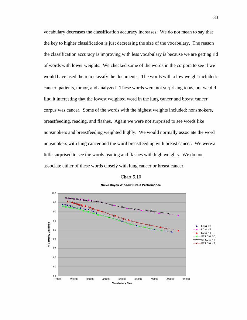
5.5 Vocabulary Analysis
We did not specifically design a test for vocabulary size, but limiting the data by
higher and higher term weights did decrease the vocabulary size. By increasing the
weight we should be getting rid of words that are less likely to help in the classification
process. Charts 5.10 and 5.11 show the performance of all tests with a window size of
three and five processed by the Naïve Bayes algorithm. These charts show that as the
33
vocabulary decreases the classification accuracy increases. We do not mean to say that
the key to higher classification is just decreasing the size of the vocabulary. The reason
the classification accuracy is improving with less vocabulary is because we are getting rid
of words with lower weights. We checked some of the words in the corpora to see if we
would have used them to classify the documents. The words with a low weight included:
cancer, patients, tumor, and analyzed. These words were not surprising to us, but we did
find it interesting that the lowest weighted word in the lung cancer and breast cancer
corpus was cancer. Some of the words with the highest weights included: nonsmokers,
breastfeeding, reading, and flashes. Again we were not surprised to see words like
nonsmokers and breastfeeding weighted highly. We would normally associate the word
nonsmokers with lung cancer and the word breastfeeding with breast cancer. We were a
little surprised to see the words reading and flashes with high weights. We do not
associate either of these words closely with lung cancer or breast cancer.
Chart 5.10 Naive Bayes Window Size 3 Performance
55
60
65
70
75
80
85
90
95
100
15000 25000 35000 45000 55000 65000 75000 85000 95000
Vocabulary Size
% C
orre
ctly
Cla
ssifi
ed
LC & BCLC & HTLC & NTST LC & BCST LC & HTST LC & NT

34
Chart 5.11
Naive Bayes Window Size 5 Performance
55
60
65
70
75
80
85
90
95
100
15000 25000 35000 45000 55000 65000 75000 85000 95000
Vocabulary Size
% C
orre
ctly
Cla
ssifi
ed
LC vs BCLC vs HTLC vs NTST LC vs BCST LC vs HTST LC vs NT

35
6 Conclusion
Our goal was to determine the degree to which the preprocessing and
transformation steps in the knowledge discovery process influence classification
accuracy. We adjusted the vocabulary used for classification with stemming, windowing
and TF*IDF weightings.
The results of this study suggest that stemming has little impact on classification
accuracy. Using word phrases provided better classification performance than single
words with the Naïve Bayes algorithm. In contrast, the J48 algorithm performs worse
with multiple word phrases than compared to single words. The slight increase in
performance for window sizes of three and five come at an increased preprocessing time.
Thus, we recommend a window size of three. Classification accuracy increased with
higher term weights. For these corpora, a TF*IDF weight ranges greater than 15 to
greater than 20 provided the best classification accuracy in most cases.
This study also provides insight into the algorithm performance. In 12 out of 18
tests Naïve Bayes performed higher than J48, and the remaining 6 cases showed the same
classification accuracy. Thus, in these corpora the classification accuracy of Naïve Bayes
algorithm is typically better and never worse than the J48. In these experiments, we also
observed that the J48 algorithm ran out of memory even when we provided the largest
amount allowed by Java. Thus, we also recommend using the Naïve Bayes algorithm
over the J48 implementation in Weka.

36
To achieve the best classification accuracy and performance we recommend using
the Naïve Bayes algorithm. With respect to preprocessing we recommend using a stop
list and manual checks to remove data anomalies. The identification of data anomalies in
your target data may take a while, but removing them will reduce problems in later
knowledge discovery steps. With respect to transformation methods we recommend the
use of term weighting, specifically TF*IDF weights in the range of 15 to 20, and the use
of a three word window size. Although a window size of five had the highest accuracy in
most cases the small improvement over a window size of three is negligible when the
processing time is taken into account.

37
7 References
1. Apte, C., Fred Damerau, and Sholom Weiss. “Automated Learning of Decision
Rules for Text Categorization.” ACM Transactions of Information Systems 12.3
(1994): 233-251.
2. Bayes, T. “Essay towards solving a problem in the doctrine of chances.”
Philosophical Transactions of the Royal Society of London 53 (1763): 370-418.
3. Blake, C., and Wanda Pratt. “Better Rules, Fewer Features: A Semantic Approach
to Selecting Features from Text.” First IEEE International Conference on Data
Mining (ICDM'01) (2001): 59-66.
4. Dave, K., Steve Lawrence, and David Pennock. “Mining the Peanut Gallery:
Opinion Extraction and Semantic Classification of Product Reviews.”
Proceedings of the 12th international conference on World Wide Web (2003):
519-528.
5. Downie, J. Stephen. “Week3: TF IDF weighting.” Instructional Web Server 25
Sept 1997. The University of Western Ontario. Feb 2007.
<http://instruct.uwo.ca/gplis/601/week3/tfidf.html>.
6. Fayyad, U., Gregory Piatetsky-Shapiro, and Padhraic Smyth. “From Data Mining
to Knowledge Discovery in Databases.” IA Magazine 17.3 (1996): 37-54.
7. Fayyad, U., Gregroy Piatetsky-Shapiro, Padhraic Smyth, and Ramasamy
Uthurusamy. Advances in Knowledge Discovery and Data Mining. Menlo
Park/Cambridge: AAAI Press/The MIT Press, 1996.

38
8. Harman, D. “How Effective Is Suffixing?” Journal of the American Society for
Information Science 42.1 (1991): 7-15.
9. Joachims, T. “Text Categorization with Support Vector Machines: Learning with
Many Relevant Features.” Lecture Notes in Computer Science, 1398 (1998): 137-
142.
10. Kao, A., and Steve Poteet. “Report on KDD Conference 2004 Panel Discussion
Can Natural Language Processing Help Text Mining?” ACM SIGKDD
Explorations Newsletter 6.2 (2004): 132-133.
11. Lewis, D., and Marc Ringuette. “A Comparison of Two Learning Algorithms for
Text Categorization.” In Proc. of the Third Annual Symposium on Document
Analysis and Information Retrieval (1994): 81-93.
12. McCallum, A., and Kamal Nigam. “A Comparison of Event Models for Naïve
Bayes Text Classification.” Proceeding of AAAI/ICML-98 Workshop on
Learning for Text Categorization (1998): 41-48.
13. Porter, Martin. “The Porter Stemming Algorithm.” Tartarus.org. Jan 2006.
Tartarus.org. 01 Jun 2006 <http://www.tartarus.org/~martin/PorterStemmer/>.
14. Quinlan, J. C4.5: Programs for Machine Learning. San Francisco: Morgan
Kaufmann Publishers Inc., 1993.
15. Rogati, M., and Yiming Yang. “High-Performing Feature Selection for Text
Classification.” Proceedings of the eleventh international conference on
Information and knowledge management (2002): 659-661.

39
16. Sanderson, Mark. “Glasgow IDOM – IR linguistic utilities”. Computing Science
– Computing Science. University of Glasgow. 01 Jun 2006
<http://www.dcs.gla.ac.uk/idom/ir_resources/linguistic_utils/stop_words>.
17. Waegel, D., and April Kontostathis. “TextMOLE: Text Mining Operations
Library and Environment.” Proceedings of the 37th SIGCSE technical symposium
on Computer science education (2006): 553-557.
18. Weiss, S., Chidanand Apte, Fred Damerau, David Johnson, Frank Oles, Thilo
Goetz, and Thomas Hampp. “Maximizing Text-Mining Performance.” IEEE
Intelligent Systems 14.4 (1999): 63-69.
19. Witten, I., and Eibe Frank. Data Mining: Practical machine learning tools and
techniques. 2nd Edition. San Francisco: Morgan Kaufmann, 2005.
20. Yang, Y. “An Evaluation of Statistical Approaches to MEDLINE Indexing.”
Proceedings of AMIA-96, Fall Symposium of the American Medical Informatics
Association (1996): 358-362.
21. Yang, Y., and Jan Pedersen. “A Comparative Study on Feature Selection in Text
Categorization.” Proceedings of ICML-97, 14th International Conference on
Machine Learning (1997): 412-420.
22. Yang, Y., and Xin Liu. “A re-examination of text categorization methods.”
Proceedings of the 22nd Annual International ACM SIGIR Conference on
Research and Development in Information Retrieval (1999): 42-49.
23. Zaiane, O., and Maria-Luiza Antonie. “Classifying Text Documents by
Associating Terms with Text Categories.” Proceedings of the thirteenth
Australasian conference on Database technologies 5 (2002): 215-222.

40
Appendix A: Journals Used in Selection Criteria

41

42

43

44

45

46

47
Appendix B: Special Characters Replaced
= , ) ( > < : ; % ' " & $ * + / . [ ]

48
Appendix C: Contents of Anomaly File
-- - -year -month -years -hour -mm -hours -hr -hrs -months -week -weeks -day -days -min -mins -minute -minutes -cm -yr-old -yrs-old -week-old -weeks-old -year-old -years-old -month-old -months-old -year-young -years-young -kg -mg