bounds for the ratio of two gamma functions

Hindawi Publishing CorporationJournal of Inequalities and ApplicationsVolume 2010, Article ID 493058, 84 pagesdoi:10.1155/2010/493058

Review ArticleBounds for the Ratio of Two Gamma Functions

Feng Qi

Department of Mathematics, College of Science, Tianjin Polytechnic University, Tianjin City 300160, China

Correspondence should be addressed to Feng Qi, [email protected], [email protected]

Received 28 July 2009; Accepted 16 January 2010

Academic Editor: Laszlo Losonczi

Copyright q 2010 Feng Qi. This is an open access article distributed under the Creative CommonsAttribution License, which permits unrestricted use, distribution, and reproduction in anymedium, provided the original work is properly cited.

By looking back at the long history of bounding the ratio Γ(x + a)/Γ(x + b) for x > −min{a, b} anda, b ∈ R, various origins of this topic are clarified, several developed courses are followed, differentresults are compared, useful methods are summarized, new advances are presented, some relatedproblems are pointed out, and related references are collected.

1. Basic Definitions and Notations

In order to fluently and smoothly understand what follows in this paper, some basic conceptsand notations need to be stated at first in this section.

1.1. The Gamma Function and Related Formulas

1.1.1. The Gamma Function

It is well known that the classical Euler gamma function can be defined for x > 0 by

Γ(x) =∫∞

0tx−1e−tdt, (1.1)

the logarithmic derivative of Γ(x) is called the psi or digamma function and denoted by ψ(x),and ψ(k)(x) for k ∈ N are called the polygamma functions.

It is general knowledge that

Γ(x + 1) = xΓ(x), x > 0. (1.2)

mailto:[email protected], [email protected]

2 Journal of Inequalities and Applications

Taking the logarithm and differentiating on both sides of (1.2) give

ψ(x + 1) = ψ(x) +1x, x > 0. (1.3)

1.1.2. Stirling’s Formula

For x > 0, there exists 0 < θ < 1 such that

Γ(x + 1) =√

2π xx+1/2 exp(−x +

θ

12x

). (1.4)

See [1, page 257, 6.1.38].

1.1.3. Wallis Cosine Formula

Wallis cosine or sine formula reads [2] that

∫π/2

0cosnxdx =

∫π/2

0sinnxdx

=√π Γ((n + 1)/2)

nΓ(n/2)=

⎧⎪⎪⎪⎨⎪⎪⎪⎩

π

2· (n − 1)!!

n!!for n even,

(n − 1)!!n!!

for n odd,

(1.5)

where n!! denotes a double factorial. Therefore,

(2k)!!(2k − 1)!!

=√π Γ(k + 1)Γ(k + 1/2)

, k ∈ N. (1.6)

1.1.4. Duplication Formula

For x > 0,

2x−1Γ(x

2

)Γ(x + 1

2

)=√π Γ(x). (1.7)

1.1.5. Binet’s First Formula

Binet’s first formula for lnΓ(x) is given by

ln Γ(x) =(x − 1

2

)lnx − x + ln

√2π + θ(x) (1.8)

Journal of Inequalities and Applications 3

for x > 0, where

θ(x) =∫∞

0

(1

et − 1− 1

t+

12

)e−xt

tdt (1.9)

for x > 0 is called the remainder of Binet’s first formula for the logarithm of the gammafunction. See [3, page 11].

1.1.6. Wendel’s Limit

For real numbers a and b,

limx→∞

[xb−a Γ(x + a)

Γ(x + b)

]= 1. (1.10)

See [1, page 257, 6.1.46].If z/= − a,−a − 1, . . . and z/= − b,−b − 1, . . . , then

zb−aΓ(z + a)Γ(z + b)

∼ 1 +(a − b)(a + b − 1)

2z+(a − b)(a − b − 1)

[3(a + b − 1)2 − a + b − 1

]24z2

+ · · ·

(1.11)

as z → ∞ along any curve joining z = 0 and z = ∞. See [4, pages 118-119].

1.1.7. Legendre’s Formula

For x > 0,

ψ(x) = −γ +∫1

0

tx−1 − 1t − 1

dt. (1.12)

1.1.8. Gauss’ Theorem

For Re(c − a − b) > 0,

∞∑n=0

(a)n(b)nn!(c)n

= 2F1(a, b; c; 1) =Γ(c)Γ(c − a − b)Γ(c − a)Γ(c − b)

. (1.13)

See [5, page 66, Theorem 2.2].


1.2. The q-Gamma Function and Related Formulas

It is well known (see [5, pages 493–496] and [6]) that the q-gamma function, the q-analogueof the gamma function Γ(x), is defined for x > 0 by

Γq(x) =(1 − q

)1−x∞∏i=0

1 − qi+1

1 − qi+x(1.14)

for 0 < q < 1 and

Γq(x) =(q − 1

)1−xq

(x

2

)∞∏i=0

1 − q−(i+1)

1 − q−(i+x)(1.15)

for q > 1. It has the following basic properties

limq→ 1+

Γq(z) = limq→ 1−

Γq(z) = Γ(z), Γq(x) = q

(x−1

2

)Γ1/q(x). (1.16)

The q-psi function ψq(x), the q-analogue of the psi function ψ(x), for 0 < q < 1 and x > 0 maybe defined by

ψq(x) =Γ′q(x)

Γq(x)= − ln

(1 − q

)+ ln q

∞∑k=0

qk+x

1 − qk+x= − ln

(1 − q

)+ ln q

∞∑k=1

qkx

1 − qk, (1.17)

and ψ(k)q (x), the q-analogues of the polygamma functions ψ(k)(x), for k ∈ N are called the

q-polygamma functions. The following Stieltjes integral representation for ψq(x) is given in[7]:

ψq(x) = − ln(1 − q

)−∫∞

0

e−xt

1 − e−tdγq(t) (1.18)

for 0 < q < 1 and x > 0, where

γq(t) = − ln q∞∑k=1

δ(t + k ln q

). (1.19)

1.3. Logarithmically Convex Functions

Definition 1.1 (see [8, 9]). For k ∈ N, a positive and k-time differentiable function f(x) is saidto be k-log-convex on an interval I if

[ln f(x)

](k) ≥ 0 (1.20)

on I. If the inequality (1.20) is reversed, then f is said to be k-log-concave on I.


Remark 1.2. It is clear that a 1-log-convex function (or 1-log-concave function, resp.) isequivalent to a positive and increasing (or decreasing, resp.) function and that a 2-log-convexfunction is positive and convex. Conversely, a convex function may not be 2-log-convex. See[8, page 7, Remark 1.16].

1.4. Completely Monotonic Functions

Definition 1.3 ([10, Chapter XIII] and [11, Chapter IV]). A function f is said to be completelymonotonic on an interval I if f has derivatives of all orders on I and

(−1)nf (n)(x) ≥ 0 (1.21)

for x ∈ I and n ≥ 0.

Remark 1.4. The famous Bernstein-Widder’s Theorem [11, page 161] states that a function fis completely monotonic on (0,∞) if and only if

f(x) =∫∞

0e−xsdμ(s), (1.22)

where μ is a nonnegative measure on [0,∞) such that the integral (1.22) converges for allx > 0. This means that a completely monotonic function f on (0,∞) is a Laplace transform ofthe measure μ.

Remark 1.5. A result of [12, page 98] asserts that for a completely monotonic function f on(a,∞), inequalities in (1.21) strictly hold unless f(x) is constant. This assertion can also befound in [13].

Definition 1.6 (see [14]). If f (k)(x) for some nonnegative integer k is completely monotonic onan interval I, but f (k−1)(x) is not completely monotonic on I, then f(x) is called a completelymonotonic function of the kth order on an interval I.

1.5. Logarithmically Completely Monotonic Functions

Definition 1.7 (see [14, 15]). A positive function f is said to be logarithmically completelymonotonic on an interval I ⊆ R if it has derivatives of all orders on I and its logarithm ln fsatisfies

(−1)k[ln f(x)

](k) ≥ 0 (1.23)

for k ∈ N on I.


Remark 1.8. In [15–19], it was recovered that any logarithmically completely monotonicfunction f on I must be completely monotonic on I, but not conversely. However, itwas discovered in [20, Section 5] that every completely monotonic function on (0,∞) islogarithmically convex.

Remark 1.9. The following conclusions may be useful: A logarithmically convex function isalso convex. If f is nonnegative and concave, then it is logarithmically concave. The sum offinite logarithmically convex functions is also a logarithmically convex function. But, the sumof two logarithmically concave functions may not be logarithmically concave. See [20, Section3].

Remark 1.10. In [16, Theorem 1.1] and [13, 21] it is pointed out that the logarithmicallycompletely monotonic functions on (0,∞) can be characterized as the infinitely divisiblecompletely monotonic functions studied by Horn in [22, Theorem 4.4] and that the set of allStieltjes transforms is a subset of the set of logarithmically completely monotonic functionson (0,∞).

Remark 1.11. For more information on characterizations, applications and history of theclass of logarithmically completely monotonic functions, please refer to [13–17] and relatedreferences therein.

Definition 1.12 (see [23, 24]). Let f be a positive function which has derivatives of all orderson an interval I. If [ln f(x)](k) for some nonnegative integer k is completely monotonic onI, but [ln f(x)](k−1) is not completely monotonic on I, then f is said to be a logarithmicallycompletely monotonic function of the kth order on I.

Definition 1.13 (see [11, 25]). A function f is said to be absolutely monotonic on an interval Iif it has derivatives of all orders and

f (k−1)(t) ≥ 0 (1.24)

for t ∈ I and k ∈ N.

Definition 1.14 (see [23, 24]). Let f be a positive function which has derivatives of all orderson an interval I. If [ln f(x)](k) for some nonnegative integer k is absolutely monotonic onI, but [ln f(x)](k−1) is not absolutely monotonic on I, then f is said to be a logarithmicallyabsolutely monotonic function of the kth order on I.

Definition 1.15 (see [23, 24]). A positive function f which has derivatives of all orders on aninterval I is said to be logarithmically absolutely convex on I if

[ln f(x)

](2k) ≥ 0 (1.25)

on I for k ∈ N.


1.6. Some Useful Formulas and Inequalities

1.6.1. Jensen’s Inequality

If φ is a convex function on [a, b], then

φ

(n∑

k=1

pkxk

)≤

n∑k=1

pkφ(xk), (1.26)

where n ∈ N, xk ∈ [a, b], and pk ≥ 0 for 1 ≤ k ≤ n satisfying∑n

k=1 pk = 1.

1.6.2. Holder’s Inequality for Integrals

Let p and q be positive numbers satisfying 1/p + 1/q = 1. If f and g are absolutely integrableon (0,∞), then

∫∞

0

∣∣f(t)g(t)∣∣dt ≤[∫∞

0

∣∣f(t)∣∣pdt]1/p[∫∞

0

∣∣g(t)∣∣qdt]1/q

, (1.27)

with equality when |g(x)| = c|f(x)|p−1.

1.6.3. Convolution Theorem of Laplace Transform (See [26])

Let fi(t) for i = 1, 2 be piecewise continuous in arbitrary finite intervals included on (0,∞). Ifthere exist some constants Mi > 0 and ci ≥ 0 such that |fi(t)| ≤ Mie

cit for i = 1, 2, then

∫∞

0

[∫ t

0f1(u)f2(t − u)du

]e−stdt =

∫∞

0f1(u)e−sudu

∫∞

0f2(v)e−svdv. (1.28)

1.6.4. Mean Values

The generalized logarithmic mean Lp(a, b) of order p ∈ R for positive numbers a and b witha/= b is defined in [27, page 385] by

Lp(a, b) =

⎧⎪⎪⎪⎪⎪⎪⎪⎪⎪⎪⎪⎪⎨⎪⎪⎪⎪⎪⎪⎪⎪⎪⎪⎪⎪⎩

[bp+1 − ap+1(p + 1

)(b − a)

]1/p

p /= − 1, 0,

b − a

ln b − lnap = −1,

1e

(bb

aa

)1/(b−a)

p = 0.

(1.29)


Note that

L1(a, b) =a + b

2= A(a, b), L−1(a, b) = L(a, b), L0(a, b) = I(a, b) (1.30)

are called, respectively, the arithmetic mean, the logarithmic mean, and the identric orexponential mean in the literature. Since the generalized logarithmic mean Lp(a, b) isincreasing in p for a/= b, see [27, pages 386-387, Theorem 3], inequalities

L(a, b) < I(a, b) < A(a, b) (1.31)

are valid for a > 0 and b > 0 with a/= b. See also [25, 28, 29] and related references therein.

1.6.5. Bernoulli Numbers

Bernoulli numbers Bn for n ≥ 0 can be defined as

x

ex − 1=

∞∑n=0

Bn

n!xn = 1 − x

2+

∞∑j=1

B2jx2j(2j)!, |x| < 2π. (1.32)

The first six Bernoulli numbers are

B0 = 1, B1 = −12, B2 =

16, B4 = − 1

30, B6 =

142

, B8 = − 130

. (1.33)

1.6.6. A Completely Monotonic Function

For any real number α, let

Θα(x) = xα[lnx − ψ(x)], x ∈ (0,∞). (1.34)

The function Θ1(x) was proved in [30, Theorem 3.1] to be decreasing and convex on(0,∞).

By using Binet’s first formula (1.9) and complicated calculating techniques for properintegrals, a general result was presented in [31, pages 374-375, Theorem 1]. For real numberα, the function Θα(x) is completely monotonic on (0,∞) if and only if α ≤ 1.

Recently the completely monotonic property of Θα(x) was also proved by differentapproaches in [32–34].


1.7. Properties of A Function Involving the Exponential Function

For t ∈ R and real numbers α and β satisfying α/= β and (α, β)/∈ {(0, 1), (1, 0)}, let

qα,β(t) =

⎧⎪⎨⎪⎩

e−αt − e−βt

1 − e−t, t /= 0,

β − α, t = 0.(1.35)

In [9, 35–40], sufficient and necessary conditions that the function qα,β(x) is monotonic,logarithmically convex, and logarithmically concave on (0,∞) were discovered step by step.

1.7.1. Monotonic Properties of qα,β(x)

The earliest complete conclusions on monotonic properties of qα,β(x) were discussed in thepaper [36] little by little but thoroughly.

Theorem 1.16 (see [35, 36]). Let α and β satisfying α/= β and (α, β)/∈ {(0, 1), (1, 0)} be realnumbers and t ∈ R.

(1) The function qα,β(t) is increasing on (0,∞) if and only if

(β − α

)(1 − α − β

)≥ 0,

(β − α

)(∣∣α − β∣∣ − α − β

)≥ 0. (1.36)

(2) The function qα,β(t) is decreasing on (0,∞) if and only if

(β − α

)(1 − α − β

)≤ 0,

(β − α

)(∣∣α − β∣∣ − α − β

)≤ 0. (1.37)

(3) The function qα,β(t) is increasing on (−∞, 0) if and only if

(β − α

)(1 − α − β

)≥ 0,

(β − α

)(2 −∣∣α − β

∣∣ − α − β)≥ 0. (1.38)

(4) The function qα,β(t) is decreasing on (−∞, 0) if and only if

(β − α

)(1 − α − β

)≤ 0,

(β − α

)(2 −∣∣α − β

∣∣ − α − β)≤ 0. (1.39)

(5) The function qα,β(t) is increasing on (−∞,∞) if and only if

(β − α

)(∣∣α − β∣∣ − α − β

)≥ 0,

(β − α

)(2 −∣∣α − β

∣∣ − α − β)≥ 0. (1.40)

(6) The function qα,β(t) is decreasing on (−∞,∞) if and only if

(β − α

)(∣∣α − β∣∣ − α − β

)≤ 0,

(β − α

)(2 −∣∣α − β

∣∣ − α − β)≤ 0. (1.41)


β

β = α + 1

β = α β = α − 1

O 1

α

1

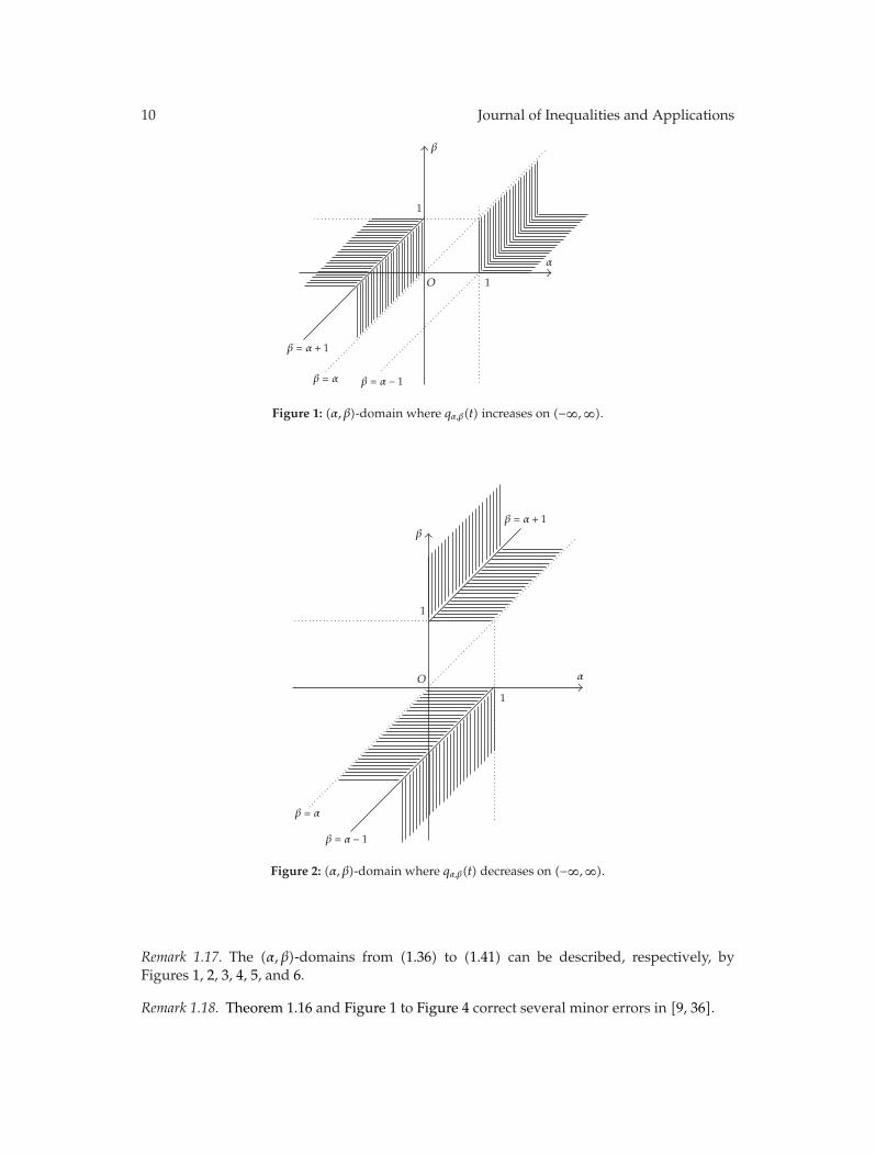
Figure 1: (α, β)-domain where qα,β(t) increases on (−∞,∞).

β

β = α

β = α − 1

O

1

α

1

β = α + 1

Figure 2: (α, β)-domain where qα,β(t) decreases on (−∞,∞).

Remark 1.17. The (α, β)-domains from (1.36) to (1.41) can be described, respectively, byFigures 1, 2, 3, 4, 5, and 6.

Remark 1.18. Theorem 1.16 and Figure 1 to Figure 4 correct several minor errors in [9, 36].


β

β = α + 1

β = α β = α − 1

β = 1 − α

O 1

α

1

Figure 3: (α, β)-domain where qα,β(t) is increasing on (0,∞).

β

β = α

β = α + 1

β = α − 1

O 1 α

1

β = 1 − α

Figure 4: (α, β)-domain where qα,β(t) is decreasing on (0,∞).

1.7.2. Logarithmically Convex Properties of qα,β(t)

These results were founded at first in [39, Lemma 1] and [40, Lemma 1] earlier thanmonotonic properties of qα,β(t).

Theorem 1.19 (see [35–40]). The function qα,β(t) on (−∞,∞) is logarithmically convex if β−α > 1and logarithmically concave if 0 < β − α < 1.


β

β = α

β = α + 1

β = α − 1

O 1

α

1

β = 1 − α

Figure 5: (α, β)-domain where qα,β(t) is increasing on (−∞, 0).

β

β = α

β = α + 1

β = α − 1

O 1 α

1

β = 1 − α

Figure 6: (α, β)-domain where qα,β(t) is decreasing on (−∞, 0).

Remark 1.20. This theorem tells us that the logarithmic convexity and logarithmic concavityof qα,β(t) on the interval (−∞, 0), showed in [39, Lemma 1] and [40, Lemma 1] , are wrong.However, this does not affect the correctness of any other results established in [39, 40], sincethe wrong conclusions about qα,β(t) on the interval (−∞, 0) are idle there luckily.


1.7.3. Three-Log-Convex Properties of qα,β(t)

Theorem 1.21 (see [9]). If 1 > β − α > 0, then qα,β(t) is 3-log-convex on (0,∞) and 3-log-concaveon (−∞, 0); if β − α > 1, then qα,β(t) is 3-log-concave on (0,∞) and 3-log-convex on (−∞, 0).

Remark 1.22. So far no application of 3-log-convex properties of qα,β(t) is disclosed, unlikemonotonic and logarithmically convex properties of qα,β(t) already having applications in[35, 37–41], respectively.

Remark 1.23. One of the key steps proving Theorems 1.16 to 1.21 is to rewrite the functionqα,β(t) as

qα,β(t) =sinh(β − α

)t/2

sinh(t/2)exp

(1 − α − β

)t

2. (1.42)

Remark 1.24. The monotonic and convex properties of qα,β(t) have important applications toinvestigations of the gamma and q-gamma functions.

2. The History and Origins

In the history of this topic, there are several independent origins and different motivations ofbounding the ratio of two gamma functions, no matter their appearances were early or late.

2.1. Wendel’s Double Inequality and Proof

As early as in 1948, in order to establish the classical asymptotic relation

limx→∞

Γ(x + s)xsΓ(x)

= 1 (2.1)

for real s and x, using Holder’s inequality (1.27), Wendel proved in [42] the double inequality

(x

x + s

)1−s≤ Γ(x + s)

xsΓ(x)≤ 1 (2.2)

for 0 < s < 1 and x > 0.

Wendel’s Proof for (2.1) and (2.2). Let

0 < s < 1, p =1s, q =

p

p − 1=

11 − s

,

f(t) = e−sttsx, g(t) = e−(1−s)tt(1−s)x+s−1,

(2.3)


and apply Holder’s inequality (1.27) and the recurrent formula (1.2) to obtain

Γ(x + s) =∫∞

0e−ttx+s−1dt ≤

(∫∞

0e−ttxdt

)s(∫∞

0e−ttx−1dt

)1−s= [Γ(x + 1)]s[Γ(x)]1−s = xsΓ(x).

(2.4)

Replacing s by 1 − s in (2.4), we get

Γ(x + 1 − s) ≤ x1−sΓ(x), (2.5)

from which we obtain

Γ(x + 1) ≤ (x + s)1−sΓ(x + s), (2.6)

by substituting x + s for x.Combining (2.4) and (2.6), we get

x

(x + s)1−s Γ(x) ≤ Γ(x + s) ≤ xsΓ(x). (2.7)

Therefore, the inequality (2.2) follows.Letting x tend to infinity in (2.2) yields (2.1) for 0 < s < 1. The extension to all real s is

immediate on repeated application of (1.2).

Remark 2.1. The inequality (2.2) can be rewritten for 0 < s < 1 and x > 0 as

x1−s ≤ Γ(x + 1)Γ(x + s)

≤ (x + s)1−s. (2.8)

Remark 2.2. The limits (1.10) and (2.1) are equivalent to each other, since

xt−s Γ(x + s)Γ(x + t)

=Γ(x + s)xsΓ(x)

· xtΓ(x)Γ(x + t)

. (2.9)

Hence, the limit (1.10) is called Wendel’s limit in the literature of this paper.

Remark 2.3. The double inequality (2.2) or (2.8) is more meaningful than the limit (2.1), sincethe former implies the latter, but not conversely.

Remark 2.4. Due to unknown reasons, Wendel’s paper [42] and inequalities (2.2) or (2.8) werepossibly neglected by nearly all mathematicians for about more than fifty years, until 1999 in[43] and later in [20, 44–49], to the best of my knowledge.


2.2. Gurland’s Upper Bound

In 1956, by a basic theorem in mathematical statistics concerning unbiased estimators withminimum variance, Gurland in [50, page 645] established a closer approximation to π

4k + 3

(2k + 1)2

[(2k)!!

(2k − 1)!!

]2

< π <4

4k + 1

[(2k)!!

(2k − 1)!!

]2

, k ∈ N (2.10)

through presenting

[Γ((n + 1)/2)

Γ(n/2)

]2

<n2

2n + 1, n ∈ N. (2.11)

Remark 2.5. The double inequality (2.10) may be rearranged as

√4k + 3√

π (2k + 1)<

(2k − 1)!!(2k)!!

<2√

π(4k + 1), k ∈ N. (2.12)

Remark 2.6. The inequality (2.11) is better than the right-hand side inequality in (2.8) forx = (n − 1)/2 and s = 1/2.

Remark 2.7. Taking, respectively, n = 2k and n = 2k − 1 for k ∈ N in (2.11) leads to

√k +

14

<Γ(k + 1)

Γ(k + 1/2)<

2k√4k − 1

, k ∈ N. (2.13)

This is better than (2.8) for x = k and s = 1/2. We will see that it is also better than (2.23) fors = 1/2 and it is the same as (2.31).

Remark 2.8. It is astonishing that inequalities in (2.11) or (2.12) were recovered in [51] by adifferent but elementary approach. In other words, the inequality (2.11) and the right-handside inequality in (2.30) are the same. See Section 2.5.

Remark 2.9. Just like the paper [42], Gurland’s paper [50] was also neglected until 1966 in[52] and 1985 in [53]. The famous monograph [54] recorded neither of the papers [42, 50].It is a pity, since inequalities in (2.10) and (2.11) are very sharp, as discussed in Remark 2.12below.

Remark 2.10. For more information on new developments of bounding Wallis’ formula (1.5),please refer to Section 7.4.


2.3. Kazarinoff’s Bounds for Wallis’ Formula

In 1956, starting from one form of the celebrated formula of John Wallis,

1√π(n + 1/2)

<(2n − 1)!!(2n)!!

<1√πn

, n ∈ N, (2.14)

which had been quoted for more than a century before 1950s by writers of textbooks, it wasproved in [55] that the sequence θ(n) defined by

(2n − 1)!!(2n)!!

=1√

π(n + θ(n))(2.15)

satisfies 1/4 < θ(n) < 1/2 for n ∈ N. This implies

1√π(n + 1/2)

<(2n − 1)!!(2n)!!

<1√

π(n + 1/4), n ∈ N. (2.16)

It was said in [55] that it is unquestionable that inequalities similar to (2.16) can beimproved indefinitely but at a sacrifice of simplicity, which is why they have survived solong.

The proof of (2.16) is based upon the property

[lnφ(t)

]′′ − {[lnφ(t)]′}2

> 0 (2.17)

of the function

φ(t) =∫π/2

0sintxdx =

√π

2Γ((t + 1)/2)Γ((t + 2)/2)

(2.18)

for −1 < t < ∞. The inequality (2.17) was proved by making use of (1.12) and estimating theintegrals

∫1

0

xt

1 + xdx,

∫1

0

xt lnx

1 + xdx. (2.19)

Since (2.17) is equivalent to the statement that the reciprocal of φ(t) has an everywherenegative second derivative, therefore, for any positive t, φ(t) is less than the harmonic meanof φ(t − 1) and φ(t + 1); simplifying this leads to the fact that

Γ((t + 1)/2)Γ((t + 2)/2)

<2√

2t + 1, t > 0. (2.20)

As a subcase of this result, the right-hand side inequality in (2.16) is established.


Remark 2.11. Replacing t by 2t for t > 0 in (2.20) leads to

Γ(t + 1/2)Γ(t + 1)

<1√

t + 1/4(2.21)

for t > 0, which is better than the left-hand side inequality in (2.8) for s = 1/2 and extends theleft-hand side inequality in (2.13).

Remark 2.12. The right-hand side inequality in (2.12) is the same as the corresponding onein (2.16), and the left-hand side inequality in (2.12) is better than the corresponding one in(2.16) and (3.6) for n ≥ 2. Therefore, Gurland’s inequality (2.11) is much sharp.

Remark 2.13. A double inequality bounding the quantity (2k − 1)!!/(2k)!! can be reduced toan upper or a lower bound for the ratio Γ((n + 1)/2)/Γ(n/2). Conversely, either the upper orthe lower bound for the ratio Γ((n + 1)/2)/Γ(n/2) can be used to derive a double inequalitybounding the quotient (2k − 1)!!/(2k)!!.

Remark 2.14. The idea and spirit of Kazarinoff in [55] would be developed by Watson in [56].See Section 3.1.

2.4. Gautschi’s Double Inequalities

In 1959, among other things, by a different motivation from Wendel in [42], Gautschiestablished independently in [57] two double inequalities for n ∈ N and 0 ≤ s ≤ 1:

n1−s ≤ Γ(n + 1)Γ(n + s)

≤ exp((1 − s)ψ(n + 1)

), (2.22)

n1−s ≤ Γ(n + 1)Γ(n + s)

≤ (n + 1)1−s. (2.23)

Remark 2.15. It is clear that the upper bound and the domain in the inequality (2.23) are notbetter and more extensive than the corresponding ones in (2.8).

Remark 2.16. The upper bounds in (2.8), (2.22), and (2.23) have the following relationships:

exp((1 − s)ψ(n + 1)

)≤ (n + 1)1−s (2.24)

for 0 < s ≤ 1 and n ∈ N,

(n + s)1−s ≤ exp((1 − s)ψ(n + 1)

)(2.25)

for 0 ≤ s ≤ 1/2 and n ∈ N, and the inequality (2.25) reverses for s > e1−γ − 1 = 0.52620 · · · ,since the function

Q(x) = eψ(x+1) − x (2.26)


was proved in [58, Theorem 2] to be strictly decreasing on (−1,∞), with

limx→∞

Q(x) =12. (2.27)

This means that Wendel’s double inequality (2.8) and Gautschi’s first double inequality (2.22)are not included in each other but they all contain Gautschi’s second double inequality (2.23).

Remark 2.17. By the convex property of lnΓ(x), Merkle recovered in [20, 59–63] inequalitiesin (2.22) and (2.23) once again. See Section 4.

Remark 2.18. The monotonic and convex properties of the function (2.27) are also derived in[64]. See Section 3.20.1 and Remark 3.56 to Remark 3.58.

Remark 2.19. The Mathematical Reviews’ comments MR0103289 on the paper [57] are citedas follows. The author gives lower and upper bounds of the form c[(xp + (1/c))1/p − x] forex

p ∫∞x e−t

pdt in the range p > 1 and 0 ≤ x < ∞; the respective values of c are 2 and [Γ(1 +

(1/p))]p/(p−1). As it stands, the proof is only valid if p is an integer, but, in a correction, theauthor has indicated a modification which validates it for all p > 1.

Remark 2.20. There is no word commenting on inequalities in (2.22) and (2.23) by theMathematical Reviews’ reviewer of the paper [57]. However, these two double inequalitieslater became a major source of a series of research on bounding the ratio of two gammafunctions.

Remark 2.21. The function exp ∫∞

x e−tpdt was further investigated in [65–72] and related

references therein.

2.5. Chu’s Double Inequality

In 1962, by discussing that bn+1(c) � bn(c) if and only if (1 − 4c)n + 1 − 3c � 0, where

bn(c) =(2n − 1)!!(2n)!!

√n + c , (2.28)

it was demonstrated in [51, Theorem 1] that

1√π[n + (n + 1)/(4n + 3)]

<(2n − 1)!!(2n)!!

<1√

π(n + 1/4), n ∈ N. (2.29)

As an application of (2.29), by using Γ(1/2) =√π and (1.2), the following double inequality

√2n − 3

4<

Γ(n/2)Γ(n/2 − 1/2)

≤

√(n − 1)2

2n − 1(2.30)

for positive integers n ≥ 2 was given in [51, Theorem 2].


Remark 2.22. After letting x = (n − 1)/2 the inequality (2.30) becomes

√x − 1

4<

Γ(x + 1/2)Γ(x)

<x√

x + 1/4, (2.31)

which is the same as (2.13).

Remark 2.23. When n is large enough, the lower bound in (2.29) is better than the one in (3.6).

Remark 2.24. Any one of the bounds in (2.31) may be derived from the other one by Boyd’smethod in [73] (see Section 3.4), by Shanbhag’s technique in [74] (see Section 3.5), by RajaRao’s technique in [75] (see Section 3.10), by Slavic’s method in [76] (see Section 3.10), or bythe β-transform in Section 4.1. This implies that the double inequality (2.30) is equivalent tothe inequality (2.11).

Remark 2.25. The double inequality (2.29) and the right-hand side inequality in (2.30) are arecovery of (2.12) and (2.11), respectively. Notice that the reasoning directions in the twopapers [50, 51] are opposite:

(2n − 1)!!(2n)!!

[51]=⇒⇐=[50]

Γ(n/2)Γ(n/2 − 1/2)

. (2.32)

This confirms again what is said in Remark 2.13.

Remark 2.26. The idea of Chu’s proof in [51, Theorem 1] has the same spirit as Kershaw’s in[77]. See Section 3.12.

2.6. Zimering’s Inequality

In 1962, Zimering obtained in [78, page 88] that

Γ(n + r)n!

≤ nr − (n − 1)r

r(2.33)

for 0 < r < 1 and n ∈ N.

Remark 2.27. From (1.2) it is easy to see that n! = Γ(n + 1). Hence, the inequality (2.33) can berearranged as

Γ(n + 1)Γ(n + r)

≥ r

nr − (n − 1)r(2.34)

for 0 < r < 1 and n ∈ N. Although the inequality (2.33) or (2.34) is not better than the left-hand side inequality in (2.22) or (2.23), since its motivation is particular, it is believed that itwas obtained independently, and so the paper [78] can also be regarded as an origin of thistopic.


2.7. Further Remarks

Remark 2.28. To the best of our knowledge and understanding, two evidences that there wasno cross-citation between them and that their motivations are different convince us to believethat the above origins are independent. Actually, the very real origin(s) may not be found outforever.

Remark 2.29. Except Wendel’s result, all inequalities above take values on N, the set of positiveintegers. In other words, only Wendel’s double inequality (2.8), the earliest result on thistopic, takes values on (0,∞), the set of real numbers.

Remark 2.30. As one will see, in the history of this topic, the works by Wendel, Gurland, andZimering did not become a source of bounding the ratio of two gamma functions.

Remark 2.31. In [53], some of the extensive previous background of the papers [55, 56] wasoutlined.

Remark 2.32. Currently, we may conclude that the very origins of bounding the ratio of twogamma functions are asymptotic analysis, estimation of Wallis’ cosine formula, estimation ofπ , and mathematical statistics.

Remark 2.33. The good bounds for the ratio of two gamma functions should satisfy one orseveral of the following criteria.

(1) The bounds should be easily computed by hand or by computers.

(2) Sharper the bounds are, better the bounds are.

(3) The bounds should be simple in form.

(4) The bounds should be beautiful in form.

(5) The bounds should be expressed by elementary functions or any other easilycalculated functions.

(6) The bounds are of some recurrent or symmetric properties.

(7) The bounds should have origin(s) and background(s).

(8) The bounds should have application(s) in mathematics or mathematical sciences.

Maybe these standards are also suitable for judging any other inequalities and estimates inmathematics.

3. Refinements and Extensions

In this section, the refinements and extensions of bounds for the ratio of two gamma functionsfrom 1959 will be collected, to the best of our ability.


3.1. Watson’s Monotonicity Result

In 1959, motivated by the result in [55], mentioned in Section 2.3, and basing on Gauss’Theorem (1.13), Watson observed in [56] that

[Γ(x + 1)]2

x[Γ(x + 1/2)]2= 2F1

(−1

2,−1

2;x; 1

)

= 1 +1

4x+

132x(x + 1)

+∞∑r=3

[(−1/2) · (1/2) · (3/2) · (r − 3/2)]2

r!x(x + 1) · · · (x + r − 1)

(3.1)

for x > −1/2, which implies that the much general function

θ(x) =[

Γ(x + 1)Γ(x + 1/2)

]2

− x, (3.2)

ever discussed in [55] or Section 2.3 as a special case θ(n) for n ∈ N, for x > −1/2 is decreasingand with

limx→∞

θ(x) =14, lim

x→ (−1/2)+θ(x) =

12. (3.3)

This apparently implies the sharp inequalities

14< θ(x) <

12

(3.4)

for x > −1/2,

√x +

14

<Γ(x + 1)

Γ(x + 1/2)≤

√x +

14+[Γ(3/4)Γ(1/4)

]2

=√x + 0.36423 · · · (3.5)

for x ≥ −1/4, and, by (1.5),

1√π(n + 4/π − 1)

≤ (2n − 1)!!(2n)!!

<1√

π(n + 1/4), n ∈ N. (3.6)

In [56], an alternative proof of the double inequality (3.4) was provided as follows. Let

f(x) =2√π

∫π/2

0cos2xtdt =

2√π

∫∞

0exp(−xt2

) t exp(−t2/2

)√

1 − exp(−t2)dt (3.7)


for x > 1/2. By using the fairly obvious inequalities

√1 − exp(−t2) ≤ t

t exp(−t2/4

)√

1 − exp(−t2)=

t√2 sinh(t2/2)

≤ 1,(3.8)

we have, for x > −1/4,

1√π

∫∞

0exp(−(x +

12

)t2)

dt < f(x) <1√π

∫∞

0exp(−(x +

14

)t2)

dt, (3.9)

that is to say

1√x + 1/2

< f(x) <1√

x + 1/4. (3.10)

Remark 3.1. In [56, page 8], the following interesting relation was provided:

x + θ(x) =x2

x − 1/2 + θ(x − 1/2)(3.11)

for appropriate ranges of values of x.

Remark 3.2. The formula (3.1) would be used in [73] to obtain the inequality (3.23).

Remark 3.3. The function θ(x) defined by (3.2) was extended and studied in [37–40, 64, 79–84]later.

Remark 3.4. It is easy to see that the inequality (3.5) extends and improves (2.8) if s = 1/2, saynothing of (2.22) and (2.23) if s = 1/2.

Remark 3.5. The left-hand side inequality in (3.6) is better than the corresponding one in (2.16)but worse than the corresponding one in (2.12) for n ≥ 2.

Remark 3.6. The double inequality (3.6) for bounding Wallis’ formula (1.5) was recovered,refined, or generalized recently in [70, 85–94] and related references therein. For moreinformation on bounds for Wallis’ formula (1.5), please refer to Sections 2.2, 2.3, and 7.4 ofthis paper.

Remark 3.7. It is easy to see that

θ(x)x

+ 1 =Γ(x)Γ(x + 1)

[Γ(x + 1/2)]2 (3.12)


which is a special case of Gurland’s ratio

T(x, y)=

Γ(x)Γ(y)

[Γ((x + y

)/2)]2 (3.13)

defined first in [95] for positive numbers x and y.The formula (3.12) reveals that bounds for Gurland’s ratio T(x, y) can be reduced to

bounds for Γ(x)/Γ(x + 1/2).For more information on bounding Gurland’s ratio, please refer to [20, 44, 96, 97] and

related references therein. However, there does not exist a general identity similar to (3.12)between Gurland’s ratio and the ratio of two gamma functions. As a result, considering thelimitation of length of this paper, new developments on Gurland’s ratio (3.13) will not beinvolved in detail.

3.2. Erber’s Inequality

Gurland proved in [95] that

[Γ(δ + α)]2

Γ(δ)Γ(δ + 2α)≤ δ

δ + α2, (3.14)

where α/= 0, α + 2δ > 0, and δ > 0. In [97], the following results were derived from the right-hand side inequality in (2.23) and (3.14).

(1) Taking in (3.14) δ = n ∈ N and α = (s + 1)/2 for s ∈ (0, 1) and rearranging lead to

Γ(n + 1)Γ(n + s)

<4(n + s)

4n + (s + 1)2

[Γ(n + 1)

Γ(n + (1 + s)/2)

]2

, 0 < s < 1, n ∈ N. (3.15)

Since 0 < (1+ s)/2 < 1, applying the right-hand side inequality in (2.23) to the ratioin the bracket yields a strengthened upper bound of (2.23)

Γ(n + 1)Γ(n + s)

<4(n + s)

4n + (s + 1)2 (n + 1)1−s, 0 < s < 1, n ∈ N. (3.16)

(2) Letting δ = n and 0 < s = α < 1 in (3.14) and using the right-hand side inequality in(2.23), then

Γ(n + s)Γ(n + 2s)

<(n + 1)1−s

n + s2, 0 < s < 1, n ∈ N. (3.17)


(3) After k + 1 iterations of the above process, it was obtained that

Γ(n + s)Γ(n + 2s)

<(n + 1)1−s

(n + s2)R(n, s, k),

Γ(n + 1)Γ(n + s)

<(n + 1)1−s

R(n, s, k),

(3.18)

where

R(n, s, k) =k∏i=0

{n +[(s + 2i+1 − 1

)/2i+1]2

n + (s + 2i − 1)/2i

}2i

(3.19)

for n, k ∈ N and 0 < s < 1.

In the final of [97], it was pointed out that it is ready to verify that the limit limk→∞R(n, s, k)exists and that it would be interesting to know the value of this infinite product in closedform.

Remark 3.8. It is easy to observe that bounds for Gurland’s ratio provide a method to refinebounds for ratio of two gamma functions. Conversely, it is also done.

3.3. Uppuluri’s Bounds

If X is a random variable defined on a probability space and E denotes the expectationoperator, then {E|X|r}1/r is a nondecreasing function of r > 0. See [98, page 156]. Using thisconclusion, the double inequality (2.8) was recovered in [99] for x > 0 and 0 ≤ s ≤ 1, whichsharpens the inequality (2.23) given in [57].

Following the same lines as in [97] or Section 3.2, after k + 1 iterations, Rao Uppulurifurther obtained in [99] that

Γ(x + 1)Γ(x + s)

<

[x +(s − 1 + 2k+1)/2k+1]1−s

R(x, s, k),

Γ(x + s)Γ(x + 2s)

<

[x +(s − 1 + 2k+1)/2k+1]1−s(x + s2)R(x, s, k)

(3.20)

for x > 0, 0 ≤ s ≤ 1, and k ∈ N, which improve inequalities (3.18).

Remark 3.9. In [74, page 48], Shanbhag pointed out that the discussion concerning (3.20) and(3.21) in [99] is misleading.


3.4. Uppuluri-Boyd’s Double Inequality

Motivated by (2.14) and the results in [50] (see Section 2.2), the following double inequalityfor m ∈ N was obtained in [52]:

(m +

14+

948m + 32

)1/2

<Γ(m + 1)

Γ(m + 1/2)<

[(m + 1/2)2

m + 3/4 + 9/(48m + 56)

]1/2

. (3.21)

In [73], the left-hand side inequality in (3.21) was pointed out to be false and it wasfurther demonstrated by using the formula (3.1) that the inequality

Γ(m + 1)Γ(m + 1/2)

>

(m +

14+

1am + b

)1/2(3.22)

is impossible to be true for all positive integers m if a < 32. Moreover, the following doubleinequality for m ∈ N was listed in [73]:

√m +

14+

132(m + 1)

<Γ(m + 1)

Γ(m + 1/2)<

m + 1/2√m + 3/4 + 1/(32m + 48)

(3.23)

by considering

Γ(m + 1)Γ(m + 1/2)

=m + 1/2

Γ(m + 3/2)/Γ(m + 1). (3.24)

Reminded by [73], the author of [52] went through the computations in finding theBhattacharya bounds in [52] and made corrections in [100]. The double inequality (3.23) wasrecovered in [100].

Remark 3.10. The technique used in (3.24) was employed once again in [76], see alsoSection 3.10, and summarized in [20] as the so-called β-transform and πn-transform, see alsoSection 4.

Remark 3.11. It is obvious that the lower bound in (3.23) is better than the corresponding onesin (2.8), (2.11) and (2.13), (2.22) and (2.23), (2.30) and (2.31), (2.33) and (2.34), and (3.5).

3.5. Shanbhag’s Inequalities

Motivated by [99], it was first pointed out in [74] that the right-hand side inequality in (2.8)may be deduced from the left-hand side inequality in (2.8) by observing

Γ((x + s) + 1)Γ((x + s) + (1 − s))

≥ (x + s)1−(1−s) ⇐⇒ (x + s)Γ(x + s)Γ(x + 1)

≥ (x + s)s. (3.25)


Then, by (2.8) and the technique stated in (3.25), a more general double inequality wasestablished:

α0(x, s) < α1(x, s) < · · · < Γ(x + 1)Γ(x + s)

< · · · < β1(x, s) < β0(x, s), (3.26)

where

αk(x, s) =(x + k)1−s(x + s + k − 1)(k)

(x + k)(k),

βk(x, s) =(x + k + s)1−s(x + s + k − 1)(k)

(x + k)(k)

(3.27)

for k ≥ 0, and

y(m) =

⎧⎨⎩

1, m = 0,

y(y − 1

)· · ·(y −m + 1

), m ≥ 1.

(3.28)

From the inequality (3.26), the following corollaries were deduced in [74].

(1) If x /∈N, then

θ0(x) < θ1(x) < · · · < γ(x) < · · · < ξ1(x) < ξ0(x), (3.29)

where

θk(x) =(x + k)x−[x]([x] + k)!

(x + k)(k+1),

ξk(x) =([x] + k + 1)x−[x]([x] + k)!

(x + k)(k+1)

(3.30)

for all nonnegative integer k and with [x] being the largest integer less than x.

(2) If 0 < s ≤ 1, then

s +1s− 1 < Γ(s) <

1s. (3.31)

(3) If x > 0, 0 < s < 1, and k is a nonnegative integer, then

η0(x, s) < η1(x, s) < · · · < Γ(x + s)Γ(x + 2s)

< · · · < ρ1(x, s) < ρ0(x, s), (3.32)


where

ηk(x, s) =(x + s + k)1−s(x + 2s + k − 1)(k)

(x + s + k)(k+1),

ρk(x, s) =(x + 2s + k)1−s(x + 2s + k − 1)(k)

(x + s + k)(k+1).

(3.33)

It was also proved in [74] that

β0(x, s) < T0(x, s) < T1(x, s) < · · · ,

ρ0(x, s) < P0(x, s) < P1(x, s) < · · · ,(3.34)

where

Tk(x, s) =

[x +(s − 1 + 2k+1)/2k+1]1−s

R(x, s, k),

Pk(x, s) =Tk(x, s)x + s2

(3.35)

for x > 0, 0 < s < 1, and k is a nonnegative integer, hence Shanbhag pointed out in [74, page48] that the discussion concerning (3.20) and (3.21) in [99] is misleading.

Remark 3.12. The method used in [74] is the same as the technique utilized in (3.24) whichhas been summarized as the πn-transform II (x, β, n) in Section 4.2.

3.6. Raja Rao’s Results

Based on [57, 74, 99] and by using Liapounoff’s inequality and probability distributionfunctions, the double inequalities (2.23) and (3.26) were recovered in [75].

It was also showed in [75] that

βk(x, s) =x + s

αk(x + s, 1 − s), (3.36)

so the inequality (3.26) can be written as

αk(x, s) ≤Γ(x + 1)Γ(x + s)

≤ x + s

αk(x + s, 1 − s). (3.37)


Moreover, the following double inequalities on the hypergeometric functions were alsoobtained in [75]:

Γ(x + 1)Γ(x + s)

(x + s + k)s−1 ≤ 2F1(−k, 1 − s;x + 1; 1) ≤ Γ(x + 1)Γ(x + s)

(x + k)s−1,

x + k

x + k + 1≤[

2F1(−k − 1, 1 − s;x + 1; 1)2F1(−k, 1 − s;x + 1; 1)

]1/(1−s)≤ x + s + k

x + s + k + 1,

(3.38)

where x > 0, 0 ≤ s ≤ 1, k = 0, 1, 2, . . . , and 2F1(a, b; c; 1) is the hypergeometric functiondefined by (1.13).

In [101–104], Raja Rao established some generalized inequalities and analogues forincomplete gamma functions, beta functions and hypergeometric functions, similar to thedouble inequality (2.8).

3.7. Keckic-Vasic’s Double Inequality

In 1971, by considering monotonic properties of

x + ln Γ(x) − x lnx + α lnx (3.39)

on (1,∞) for α = 1/2 or 1, respectively, among other things, Keckic and Vasic gave in [105,Theorem 1] the following double inequality for b > a > 1:

bb−1

aa−1ea−b <

Γ(b)Γ(a)

<bb−1/2

aa−1/2ea−b. (3.40)

Remark 3.13. Taking b = x + 1 and b = x + s in Keckic and Vasic’s double inequality (3.40)gives

(x + 1)x

(x + s)x+s−1e−(1−s) <

Γ(x + 1)Γ(x + s)

<(x + 1)x+1/2

(x + s)x+s−1/2e−(1−s) (3.41)

for 0 < s < 1 and x > 0.

Remark 3.14. In [105], inequalities in (3.40) were compared with those in (2.23), (2.30), and(2.33). For example, if taking b = n/2 and a = (n − 1)/2 and letting n be large enough, thenthe double inequality (3.40) is not sharper than (2.30), say nothing of the inequality (3.23).

Remark 3.15. For more information on extensions and refinements of the inequality (3.40),please refer to Remark 3.43 and Section 5.


3.8. Amos’ Sharp Upper Bound

In 1973, in an appendix of the paper [106], starting with the asymptotic expansion

ln Γ(z) =(z − 1

2

)ln z − z +

12

ln(2π) +1

12z− 1

360z3+ R (3.42)

for z > 0 and estimate R by the next term |R| ≤ 1/1260z5, see [1, page 257, 6.1.42], thefollowing inequality was established in [106, pages 425–427]:

[Γ(x + 1)]2

[Γ(x + 1/2)]2< x

(1 +

14x

+1

32x2− 1

128x3+

65x4

)(3.43)

for x ≥ 2. This expression is asymptotically correct in all terms except the last.

Remark 3.16. In virtue of the techniques used in [73–75], a lower bound for (3.43) can beprocured from its upper bound.

3.9. Lazarevic-Lupas’s Convexity

In 1974, among other things, the function

θα(x) =[Γ(x + 1)Γ(x + α)

]1/(1−α)− x (3.44)

on (0,∞) for α ∈ (0, 1) was claimed in [80, Theorem 2] to be decreasing and convex, and so

α

2<

[Γ(x + 1)Γ(x + α)

]1/(1−α)− x ≤ [Γ(α)]1/(1−α). (3.45)

Remark 3.17. Although Lazarevic-Lupas’s proof given in [80] on monotonic and convexproperties of θα(x) is wrong, as commented in [64, page 240], these properties are correct,as we know now.

Remark 3.18. Taking α = 1/2 in (3.44) leads to Watson’s monotonicity result in Section 3.1, butthe range of x here is slightly smaller. Note that Watson did not discuss in [56] the convexproperty of the function θ(x) defined by (3.2).

Remark 3.19. The function θα(x) would be extended and the same properties would beverified in [37–40, 64, 79]. See Sections 3.20.1 and 6.1.

Remark 3.20. It seems that the problem discussed in [80, Theorem 1] on characterization ofthe gamma function was further carried out by Merkle in [20, 59] and Lorch in [107] andrelated references therein.


3.10. Slavic’s Double Inequalities

In 1975, by virtue of (1.2), the following implications were pointed out in [76, page 19]:

f(x) ≤ Γ(x + 1)Γ(x + 1/2)

=⇒ Γ(x + 1)Γ(x + 1/2)

≤ x + 1/2f(x + 1/2)

, (3.46)

Γ(x + 1)Γ(x + 1/2)

≤ g(x) =⇒ x

g(x − 1/2)≤ Γ(x + 1)

Γ(x + 1/2). (3.47)

In particular, adopting

g(x) =

√x +

14+

132x + 8

(3.48)

in (3.47) leads to

√x +

14+

132x + 8 + 36/(4x − 1)

<Γ(x + 1)

Γ(x + 1/2)<

√x +

14+

132x + 8

. (3.49)

On basis of Duplication formula (1.7) and Binet’s first formula (1.9), the followingintegral representation was also given in [76]:

Γ(x + 1)Γ(x + 1/2)

=√x exp

{n∑

k=1

(1 − 2−2k)B2k

k(2k − 1)x2k−1×∫∞

0

[tanht

2t−

n∑k=1

22k(22k − 1)B2k

2 · (2k)! t2k−2

]e−4txdt

},

(3.50)

from which, a more accurate double inequality was procured:

√x exp

(2m∑k=1

(1 − 2−2k)B2k

k(2k − 1)x2k−1

)<

Γ(x + 1)Γ(x + 1/2)

<√x exp

(2 −1∑k=1

(1 − 2−2k)B2k

k(2k − 1)x2k−1

)(3.51)

for x > 0, where m and are natural numbers and B2k for k ∈ N are Bernoulli numbers.

Remark 3.21. Why can the function g(x) in (3.47) be taken as (3.48)? There was not any clueto it in [76], but the double inequality (3.49) is surely sound.

Remark 3.22. What are the ranges of x in the double inequalities (3.46), (3.47) and (3.49)?These were not provided explicitly in [76]. As we know now, the double inequality (3.49) isvalid for x > −1/4.

Remark 3.23. It was claimed in [76] that inequalities in (3.49) are sharper than those in (3.23)and many other inequalities mentioned above. In fact, it is true.


Remark 3.24. It was also claimed in [76] that inequalities in (3.51) are sharper than those in(3.49), but there was no proof supplied in it.

Remark 3.25. We conjecture that the constants 32 and 8 in the upper bound of (3.49) are thebest possible.

Remark 3.26. The lower bound in (3.49) would be refined by the corresponding one in (7.24)obtained in [108, Theorem 1].

Remark 3.27. The method showed by (3.46) and (3.47) had been used in [73–75] when provingthe double inequality (3.23) and it was summarized in [20] as the β-transform in Section 4.1.

3.11. Imoru’s Refinements of Inequalities by Uppuluri-Boyd and Slavic

In [109], it was obtained that

√m + θ(m) <

Γ(m + 1)Γ(m + 1/2)

<m + 1/2√

m + 1/2 + θ(m + 1/2)(3.52)

for

14< θ(m) ≤ 1

2. (3.53)

In particular,

(1) taking in (3.52)

θ(m) =14+

132(m + 1)

(3.54)

for m ∈ N leads to

√m +

14+

132(m + 1)

<Γ(m + 1)

Γ(m + 1/2)<

m + 1/2√m + 3/4 + 1/32(m + 1)

, (3.55)

an improved version of (3.23).

(2) Putting in (3.52)

θ(m) =14+

132m + 8 + 36/(4m − 1)

(3.56)

for m ∈ N yields (3.49).

(3) Letting in (3.52)

θ(m) =14+

132m + 8 + 36/(4m + 5)

(3.57)


for m ∈ N gives

√m +

14+

132m + 8 + 36/(4m + 5)

<Γ(m + 1)

Γ(m + 1/2)

<m + 1/2√

m + 3/4 + 1/4[4m + 6 + 9/(4m + 7)].

(3.58)

3.12. Kershaw’s Double Inequalities and Proofs

In 1983, motivated by the inequality (2.22) in [57], Kershaw presented in [77] the followingtwo double inequalities for 0 < s < 1 and x > 0:

(x +

s

2

)1−s<

Γ(x + 1)Γ(x + s)

<

[x − 1

2+(s +

14

)1/2]1−s

, (3.59)

exp[(1 − s)ψ

(x +

√s)]

<Γ(x + 1)Γ(x + s)

< exp[(1 − s)ψ

(x +

s + 12

)]. (3.60)

They are called in the literature Kershaw’s first and second double inequalities, respectively,although the order of these two inequalities (3.59) and (3.60) reverses the original order in[77].

Kershaw’s Proof for (3.59) and (3.60). Define the functions fα and gβ by

fα(x) =Γ(x + 1)Γ(x + s)

exp((s − 1)ψ(x + α)

),

gβ(x) =Γ(x + 1)Γ(x + s)

(x + β

)s−1(3.61)

for x > 0 and 0 < s < 1, where the parameters α and β are to be determined.It is not difficult to show, with the aid of Stirling’s formula (1.4), that

limx→∞

fα(x) = limx→∞

gβ(x) = 1. (3.62)

Now let

F(x) =fα(x)

fα(x + 1)=

x + s

x + 1exp

1 − s

x + α. (3.63)

Then

F ′(x)F(x)

= (1 − s)

(α2 − s

)+ (2α − s − 1)x

(x + 1)(x + s)(x + α)2. (3.64)


It is easy to show that

(1) if α = s1/2, then F ′(x) < 0 for x > 0,

(2) if α = (s + 1)/2, then F ′(x) > 0 for x > 0.

Consequently if α = s1/2 then F strictly decreases, and since F(x) → 1 as x → ∞ it followsthat F(x) > 1 for x > 0. But, from (3.62), this implies that fα(x) > fα(x + 1) for x > 0 and sofα(x) > fα(x + n). Take the limit as n → ∞ to give the result that fα(x) > 1, which can berewritten as the left-hand side inequality in (3.60). The corresponding upper bound can beverified by a similar argument when α = (s + 1)/2, the only difference is that in this case fαstrictly increases to unity.

To prove the double inequality (3.59) define

G(x) =gβ(x)

gβ(x + 1)=

x + s

x + 1

(x + β + 1x + β

)1−s, (3.65)

from which it follows that

G′(x)G(x)

=(1 − s)

[(β2 + β − s

)+(2β − s

)x]

(x + 1)(x + s)(x + β

)(x + β + 1

) . (3.66)

This will leads to

(1) if β = s/2, then G′(x) < 0 for x > 0,

(2) if β = −1/2 + (s + 1/4)1/2, then G′(x) > 0 for x > 0.

The same arguments which were used on F can now be used on G to give the doubleinequality (3.59).

Remark 3.28. The limits in (3.62) can also be derived by using (1.10).

Remark 3.29. Since the limits in (3.62) hold, the left-hand side inequality in (3.59) and theright-hand side inequality in (3.60) are immediate consequences of the fact that f(s+1)/2 andgs/2 are decreasing on (0,∞).

Remark 3.30. The spirit of Kershaw’s proof is similar to Chu’s in [51, Theorem 1]. See alsoSection 2.5.

Remark 3.31. The method used by Kershaw in [77] to prove (3.59) and (3.60) was utilized toconstruct many similar inequalities in several papers such as [107, 110, 111]. See Remark 3.39.

Remark 3.32. It is easy to see that the inequality (3.59) refines and extends the inequality (2.8),say nothing of (2.23).

Remark 3.33. Since the function Q(x) defined by (2.26) was proved in [58, Theorem 2] to bestrictly decreasing on (−1,∞), the functions

h1;s(x) = eψ(x+√s ) −

(x +

s

2

)= eψ(x+

√s ) −

(x +

√s − 1

)− s

2+√s − 1 (3.67)


for x > −√s and

h2;s(x) = eψ(x+(s+1)/2) −[x − 1

2+(s +

14

)1/2]

= eψ(x+(s+1)/2) −(x +

s + 12

− 1)−(s +

14

)1/2

+s

2

(3.68)

for x > −(s + 1)/2, where 0 < s < 1, are both strictly deceasing. From (2.27), it follows that

limx→∞

h1;s(x) =√s − s + 1

2< 0, lim

x→∞h2;s(x) =

s + 12

−(s +

14

)1/2

< 0 (3.69)

for 0 < s < 1. It is apparent that

h1;s(0) = eψ(√s ) − s

2� h1(s),

h2;s(0) = eψ(s+1/2) +12−(s +

14

)1/2

� h2(s)(3.70)

for 0 < s < 1. Direct computation gives

lims→ 1−

h1(s) = e−γ − 12> 0, lim

s→ 0+h2(s) = eψ(1/2) > 0. (3.71)

These calculations show that neither (3.59) nor (3.60) is the outright winner. When x is largeenough, the lower bound in (3.60) is not better than the one in (3.59), but the upper bound in(3.60) is better than the one in (3.59).

Remark 3.34. Kershaw proved in [77] that if 2x + s ≥ 1 and 0 < s < 1 then the lower bound inKershaw’s first double inequality (3.59) is an improvement over the lower bound in (3.41).

Remark 3.35. In [77], Kershaw compared his upper bounds with Erber’s inequality (3.16), butit is sure that there may be something wrong with his arguments.

3.13. Lorch’s Double Inequality

In 1984, by initially unaware utilization of Kershaw’s method in [77], see also Section 3.12,Lorch gave in [107] the following results. For nonnegative integers k ≥ 0, the upper bound inthe inequality

(k +

s

2

)s−1<

Γ(k + s)Γ(k + 1)

< (k + s)s−1 (3.72)

is valid for all s > 1, the lower bound in (3.72) is valid for 1 < s < 2, the left-hand sideinequality in (3.72) reverses for s > 2, and the double inequality (3.72) reverses for 0 < s < 1.


Remark 3.36. For 0 < s < 1, the double inequality (3.72) is not better than (3.59) for 0 < s < 1,but the range of the parameter s was extended.

Remark 3.37. In the special case in which s = 1/2, the inequalities in (3.72) had beenestablished first by Kazarinoff in [55] and then by Watson in [56]. From Watson’smonotonicity result in Section 3.1, the upper bounds in (3.59) for s = 1/2 and (3.72) maybe derived.

Remark 3.38. The motivation of Lorch in [107] was to refine an inequality for ultrasphericalpolynomials. Inequalities in (3.72) were used in [107] to obtain a very interesting sharpenedinequality for ultraspherical polynomials:

(sin θ)λ∣∣∣P (λ)

n (cos θ)∣∣∣ < 21−λ

Γ(λ)(n + λ)λ−1, (3.73)

where θ ∈ [0, π] and

P(λ)n (x) =

[n/2]∑k=0

(−1)kΓ(n − k + λ)

Γ(λ)Γ(k + 1)Γ(n − 2k + 1)(2x)n−2k (3.74)

for n ≥ 0 being an integer and λ > 0 being a real number. The inequality (3.73) refines theBernstein inequality


n (cos θ)∣∣∣ < 21−λ

Γ(λ)nλ−1 (3.75)

for n ≥ 0, 0 < λ < 1, and 0 ≤ θ ≤ π . Earlier in 1975, Durand generalized in [112] the Bernsteininequality (3.75) and, as a consequence of (23) in [112], the following inequality may bederived:


n (cos θ)∣∣∣ < Γ(n/2 + λ)

Γ(λ)Γ(n/2 + 1)(3.76)

for n ≥ 0, 0 < λ < 1 and 0 ≤ θ ≤ π . For more information on further refinements of theBernstein inequality (3.75), please refer to [113, pages 388-389] and the related referencestherein.

3.14. Laforgia’s Inequalities

In 1984, starting from [56, 57, 77, 107] and employing more carefully Kershaw’s and Lorch’smethods in [77, 107], by discussing the monotonicity of the function G(x) defined by (3.65)more delicately, Laforgia constructed in [111] a number of inequalities of the type

(x + α)s−1 <Γ(x + s)Γ(x + 1)

<(x + β

)s−1 (3.77)

for s > 0 and real number x ≥ 0.


Remark 3.39. As in [111], thorough analyses of Kershaw’s and Lorch’s methods had beencarried out continuously in [110, 114, 115] and [113, pages 389-390], respectively.

Remark 3.40. By discussing (3.63) subtly, the double inequality (3.60) was extended on s in[110, Section 5].

3.15. Dutka’s Double Inequalities

In 1985, some of the extensive previous background of the papers [55, 56] associated withbounding Wallis’s cosine formula or Wallis’ product formula was outlined in [53].

On the other hand, by using continued fraction expansions for the quotient of betafunctions, several bounds for the sequence θ(n) defined by (2.15), or the function θ(x) definedby (3.2), or the function θα(x) defined by (3.44) were established in [53]. For n ∈ N,

(1 +

12n

)1/2

<θ(n)n

+ 1 <

(1 − 1

2n

)−1/2

, (3.78)

4n + 32(8n + 5)

< θ(n) <2n

8n − 1, (3.79)

8n2 + 13n + 632n2 + 48n + 19

< θ(n) <8n + 3

8(4n + 1), (3.80)

14< θ(n) <

n + 14n + 3

, (3.81)

and inequalities in (2.10) and (2.29) were recovered.

Remark 3.41. The left-hand side inequalities in (3.4) and (3.79) are better than the one in (3.78),the right-hand side inequalities in (3.78) and (3.79) are better than the corresponding one in(3.4), and the right-hand side inequality in (3.79) is better than the corresponding one in(3.78).

3.16. Ismail-Lorch-Muldoon’s Monotonicity Results

In 1986, the logarithmically complete monotonicity of three functions related to the gammafunction or its ratio were obtained in [116, Theorems 2.1, 2.4, and 2.6].

(1) The function

xαΓ(x)( ex

)x(3.82)

is logarithmically completely monotonic on (0,∞) if and only if α ≤ 1/2, so is thereciprocal of the function (3.82) if and only if α ≥ 1.


(2) The function

xb−a Γ(x + a)Γ(x + b)

(3.83)

for a > b ≥ 0 is logarithmically completely monotonic on (0,∞) if and only ifa + b ≥ 1.

(3) Let

txδ

Γ(xδ + 1

) = e−h(x) (3.84)

for 0 < t ≤ e−γ .

(a) For 0 < δ ≤ 1/2, the function h(x) is positive and h′(x) is completelymonotonic on (0,∞).

(b) For δ = 1, the functions h(x) and h′(x) are both positive and h′′(x) iscompletely monotonic on (0,∞).

It was conjectured in [116, page 8] that h′′(x) remains completely monotonic for at least somevalues of δ > 1.

Remark 3.42. The logarithmically complete monotonicity of the function (3.82) was alsoproved in [117, Theorem 2.1] early in 1978. See also [7, Theorem 2.1].

Remark 3.43. It is clear that the logarithm of the function (3.82) for α = 1/2 or 1 equals thefunction (3.39). Therefore, the monotonic properties of the function (3.82) may be used toderive the double inequality (3.40) for b > a > 0 and to show the best possibilities of theconstants 1/2 and 1 in (3.40).

Remark 3.44. Since the limit (1.10) is valid, from the decreasingly monotonic property of thefunction (3.83), it follows that

xa−b <Γ(x + a)Γ(x + b)

<xa−b

xa−b0

· Γ(x0 + a)Γ(x0 + b)

(3.85)

for a > b ≥ 0 and a + b ≥ 1 holds on [x0,∞) for any x0 > 0. It is obvious that this extends theleft-hand side inequalities in (2.8), (2.22), and (2.23).

Remark 3.45. The conclusions in [116], mentioned above, were not stated using theterminology “logarithmically completely monotonic function”, since the authors were notaware of the paper [14] and related papers such as [13, 15–19, 118] have not been publishedthen.

3.17. Bustoz-Ismail’s Monotonicity Results

In 1986, it was revealed in [96] that


(1) the function

f(x) =1

(x + c)1/2· Γ(x + 1)Γ(x + 1/2)

, x > max{−1

2,−c}

(3.86)

is logarithmically completely monotonic on (−c,∞) if c ≤ 1/4, so is the reciprocalof (3.86) on [−1/2,∞) if c ≥ 1/2;

(2) the function

(x + c)a−bΓ(x + b)Γ(x + a)

(3.87)

for 1 ≥ b − a > 0 is logarithmically completely monotonic on the interval(max{−a,−c},∞) if c ≤ (a+b)−1/2, so is the reciprocal of (3.87) on (max{−b,−c},∞)if c ≥ a;

(3) the functions

Γ(x + s)Γ(x + 1)

exp[(1 − s)ψ

(x +

s + 12

)], (3.88)

Γ(x + 1)Γ(x + s)

(x +

s

2

)s−1(3.89)

for 0 < s < 1 are logarithmically completely monotonic on (0,∞);

(4) the functions

Γ(x + 1)Γ(x + s)

exp((s − 1)ψ

(x +

√s)), (3.90)

⎛⎝x − 1

2+

√s +

14

⎞⎠

1−sΓ(x + s)Γ(x + 1)

(3.91)

for 0 < s < 1 are strictly decreasing on (0,∞).

Remark 3.46. The monotonic properties of the function (3.86) implies inequalities (3.4) and(3.79).

Remark 3.47. These monotonicity results generalize, extend, and refine inequalities (2.8),(2.22), (2.23), (3.59), (3.60), monotonic properties of the function (3.83), and so on.

3.18. Alzer’s Monotonicity Result

In 1993, it was obtained in [119, Theorem 1] that

Γ(x + s)Γ(x + 1)

(x + 1)x+1/2

(x + s)x+s−1/2exp(s − 1 +

ψ ′(x + 1 + α) − ψ ′(x + s + α)12

)(3.92)


for α > 0 and s ∈ (0, 1) is logarithmically completely monotonic on (0,∞) if and only ifα ≥ 1/2, so is the reciprocal of (3.92) for α ≥ 0 and s ∈ (0, 1) if and only if α = 0.

In [120, Theorem 3], a slight extension of [119, Theorem 1] was presented. The function

Γ(x + s)Γ(x + t)

(x + t)x+t−1/2

(x + s)x+s−1/2exp(s − t +

ψ ′(x + t + α) − ψ ′(x + s + α)12

)(3.93)

for 0 < s < t and x ∈ (0,∞) is logarithmically completely monotonic if and only if α ≥ 1/2, sois the reciprocal of (3.93) if and only if α = 0.

The decreasingly monotonic properties of (3.93) and its reciprocal imply that

exp

(t − s +

ψ ′(x + s + β)− ψ ′(x + t + β

)12

)≤ Γ(x + s)

Γ(x + t)(x + t)x+t−1/2

(x + s)x+s−1/2

≤ exp(t − s +

ψ ′(x + s + α) − ψ ′(x + t + α)12

)

(3.94)

for α > β ≥ 0 are valid for 0 < s < t and x ∈ (0,∞) if and only if β = 0 and α ≥ 1/2.

Remark 3.48. The inequality (3.94) is a slight extension of the double inequality (2.6) in [119,Corollary 2].

Remark 3.49. In [119, Theorem 4], Keckic-Vasic’s double inequality (3.40) for b > a > 1 wasrefined and sharpened. For detailed information, see Section 5.2.

3.19. Ismail-Muldoon’s Monotonicity Result

In 1994, it was obtained in [7, Corollary 2.4] that, for a > 0, the function

xα−xΓ(x)(x + a)α−x−aΓ(x + a)

(3.95)

is logarithmically completely monotonic on (0,∞) if and only if α ≤ 1/2, so is the reciprocalof (3.95) if and only if α ≥ 1.

3.20. Elezovic-Giordano-Pecaric’s Results

3.20.1. The First Result

A standard argument shows that inequality (3.59) can be rearranged as

s

2<

[Γ(x + 1)Γ(x + s)

]1/(1−s)− x <

√s +

14

− 12. (3.96)


Therefore, monotonic and convex properties of the general function

zs,t(x) =

⎧⎪⎪⎨⎪⎪⎩

[Γ(x + t)Γ(x + s)

]1/(t−s)− x, s /= t,

eψ(x+s) − x, s = t

(3.97)

for x ∈ (−α,∞), where s and t are two real numbers and α = min{s, t} was considered in [64,Theorem 1] and obtained by the following theorem.

Theorem 3.50. The function zs,t(x) is either convex and decreasing for |t − s| < 1 or concave andincreasing for |t − s| > 1.

As consequences of Theorem 3.50, the following useful conclusions are derived.

(1) The function

eψ(x+t) − x (3.98)

for all t > 0 is decreasing and convex from (0,∞) onto (eψ(t), t − (1/2)).

(2) For all x > 0,

ψ ′(x)eψ(x) < 1. (3.99)

(3) For all x > 0 and t > 0,

ln(x + t − 1

2

)< ψ(x + t) < ln

(x + eψ(t)

). (3.100)

(4) For x > −α, the inequality

[Γ(x + t)Γ(x + s)

]1/(t−s)<

t − s

ψ(x + t) − ψ(x + s)(3.101)

holds if |t − s| < 1 and reverses if |t − s| > 1.

Remark 3.51. Direct computation yields

z′′s,t(x)

zs,t(x) + x=[ψ(x + t) − ψ(x + s)

t − s

]2

+ψ ′(x + t) − ψ ′(x + s)

t − s. (3.102)

To prove the positivity of the function (3.102), the following formula and inequality are usedas basic tools in the proof of the following [64, Theorem 1].


(1) For x > −1,

ψ(x + 1) = −γ +∞∑k=1

(1k− 1x + k

). (3.103)

(2) If a ≤ b < c ≤ d, then

1ab

+1cd

>1ac

+1bd

. (3.104)

Remark 3.52. In [39, 40], a new proof for [64, Theorem 1] was supplied by making use of(1.28) and Theorem 1.19 on the logarithmically convex properties of qα,β(t).

Note that a similar proof to [39, 40] for [64, Theorem 1] in the case of |t − s| < 1 wasalso given in [79].

Remark 3.53. Actually, the function (3.102) is completely monotonic under some conditionsabout s and t. This was verified in [81–84], and so several new proofs for [64, Theorem 1]were supplied again; see Section 6.2.

Remark 3.54. Inequality (3.99) was recovered in [121, Lemma 1.2].

Remark 3.55. It is easy to see that Elezovic-Giordano-Pecaric’s first main result generalizesWatson’s monotonicity result in [56] and Lazarevic-Lupas’s convexity result in [80]; seeSections 3.1 and 3.9.

Remark 3.56. In fact, function (3.98) is deceasing and convex on (−t,∞) for all t ∈ R; see [58,Theorem 2].

Remark 3.57. It is clear that the double inequality (3.100) can be deduced directly from thedecreasingly monotonic property of (3.98). Furthermore, from the decreasingly monotonicand convex properties of (3.98) on (−t,∞), inequality (3.99) and

ψ ′′(x) +[ψ ′(x)

]2> 0 (3.105)

on (0,∞) can be derived straightforwardly.

Remark 3.58. Inequalities (3.99) and (3.105) were recovered [122, page 208] and [121, Lemma1.1]. Inequality (3.105) has been generalized to the q-analogues in [123, Lemma 4.6] and to thecomplete monotonicity of divided differences of ψ(x) and ψ ′(x) in [81–84]; see Section 6.2.

3.20.2. The Second Result

It is easy to see that inequality (3.60) can be rewritten for s ∈ (0, 1) and x ≥ 1 as

exp[ψ(x +

√s)]

<

[Γ(x + 1)Γ(x + s)

]1/(1−s)< exp

[ψ

(x +

s + 12

)]. (3.106)


Now it is natural to ask: What are the best constants δ1(s, t) and δ2(s, t) such that

exp[ψ(x + δ1(s, t))

]≤[Γ(x + t)Γ(x + s)

]1/(t−s)≤ exp

[ψ(x + δ2(s, t))

](3.107)

holds for x > −min{s, t, δ1(s, t), δ2(s, t)}? where s and t are two real numbers.Elezovic-Giordano-Pecaric’s answer is the following [64, Theorem 4]. If the integral

ψ-mean of s and t is denoted by

Iψ = Iψ(s, t) = ψ−1

(1

t − s

∫ t

s

ψ(u)du

), (3.108)

then the inequality

ψ(x + Iψ(s, t)

)<

1t − s

∫ t

s

ψ(x + u)du < ψ

(x +

s + t

2

)(3.109)

is valid for every x ≥ 0 and positive numbers s and t.

Remark 3.59. It is clear that Elezovic-Giordano-Pecaric’s second main result [64, Theorem 4]is not the outright winner surely, since the ranges of s and t in (3.109) are restricted to bepositive and the lower bound in (3.109) cannot be calculated easily.

Remark 3.60. The question (3.107) was also investigated in [124–127] and has beengeneralized in [128–133]; see Section 6.4.1 and Section 6.4.2.

3.20.3. The Third Result

The function (3.88) and its monotonicity were generalized in [64, Theorem 5] and [39,Proposition 5] and [40, Proposition 5] as follows. The function

[Γ(x + t)Γ(x + s)

]1/(s−t)exp(ψ

(x +

s + t

2

))(3.110)

is logarithmically completely monotonic for x ∈ (−α,∞), where s and t are two real numbersand α = min{s, t}.

Remark 3.61. In [39, Proposition 5] and [40, Proposition 5], as a consequence of thelogarithmically complete property of the function (3.110), the right-hand side inequality in(3.106) was extended as

exp[ψ

(x +

s + t

2

)]>

[Γ(x + t)Γ(x + s)

]1/(t−s). (3.111)


3.21. Some Results from the Viewpoint of Means

It may be worthwhile mentioning the paper [134, 135] in which some monotonicity andinequalities for the gamma and incomplete gamma functions were constructed by usingproperties of extended mean values E(r, s;x, y) or generalized weighted mean valuesMf,g(r, s;x, y). For example, the inequality

eγx < Γ(x + 1) < exψ(x+1) (3.112)

is valid for x > 0 and the functions

[Γ(s, x)Γ(r, x)

]1/(s−r),

[γ(s, x)γ(r, x)

]1/(s−r)(3.113)

are increasing in r > 0, s > 0 and x > 0, where Γ(s, x) and γ(s, x) denote the incompletegamma functions with usual notation.

Remark 3.62. The right-hand side inequality in (3.112) is valid for x > −1 and takes an equalityat x = 0. Moreover, it can be rearranged by (1.2) and (1.3) as

xΓ(x) ≤ exψ(x)+1, x > −1. (3.114)

But this inequality is not better than those in [136] for bounding the gamma function Γ(x).

3.22. Batir’s Double Inequality

It is clear that the double inequality (3.60) can be rearranged as

ψ(x +

√s)<

ln Γ(x + 1) − ln Γ(x + s)1 − s

< ψ

(x +

s + 12

)(3.115)

for 0 < s < 1 and x > 1. The middle term in (3.115) can be regarded as a divided differenceof the function lnΓ(t) on the interval (x + s, x + 1). Motivated by this, Batir generalized andextended in [137, Theorem 2.7] the double inequality (3.115) as

−∣∣∣ψ(n+1)(L−(n+2)

(x, y))∣∣∣ <

∣∣ψ(n)(x)∣∣ − ∣∣ψ(n)(y)∣∣x − y

< −∣∣∣ψ(n+1)(A(x, y))∣∣∣ (3.116)

which bounds the divided differences of the polygamma functions, where x and y arepositive numbers, n a positive integer, A(x, y) and Lp(a, b) are defined by (1.29).

Remark 3.63. In [138, Theorem 2.4], the following incorrect double inequality was obtained:

e(x−y)ψ(L(x+1,y+1)−1) ≤ Γ(x)Γ(y) ≤ e(x−y)ψ(A(x,y)), (3.117)


where x and y are positive real numbers, and L(x, y) and A(x, y) are mean values defined inSection 1.6.4.

Remark 3.64. Inequalities in (3.116) and (3.117) have been corrected and refined in [128–133],respectively. See Section 6.4.2.


Remark 3.65. In [139, 140], by using a method of the geometric convexity for functions,the authors presented some known and new results on the ratio of two gamma functions,including a refinement of (3.6).

Remark 3.66. In [141], the authors investigated some general cases seemingly related with theratio of two gamma functions but essentially similar to the f-means in [142] and some resultsappeared in [121, 137, 138].

4. Merkle’s Methods and Inequalities

It is known that Merkle did many researches on bounding the ratio of two gamma functionsand has his own particular methods, approaches, and notations; therefore, this section isdevoted to summarize his results and to present his methods on this topic.

Merkle himself said in [20] that his method is founded on certain general convexityresults, as well as on integral representations of error terms in some classical and relatedinequalities.

4.1. The β-Transform

This transform has been known since [73–76]; see inequality (3.23) in Section 3.4 andinequalities (3.46) and (3.47) in Section 3.10.

The inequality

A(x, β)≤

Γ(x + β

)Γ(x)

(4.1)

implies, replacing x by x + β and β by 1 − β,

A(x + β, 1 − β

)≤ Γ(x + 1)

Γ(x + β

) , (4.2)

and therefore

Γ(x + β

)Γ(x)

≤ x

A(x + β, 1 − β

) , (4.3)

so, only the lower bound (4.1) is enough, or vice versa. It is said that inequality (4.3) is derivedfrom (4.1) by a β-transform.


4.2. The πn-Transform

This transform was firstly applied in [74, 75], see also Sections 3.5 and 3.6. It works forinequalities of both the ratio of two gamma functions and Gurland’s ratio.

For n ∈ N, let

II(x, β, n

)=

x(x + 1) · · · (x + n − 1)(x + β

)(x + β + 1

)· · ·(x + β + n − 1

) . (4.4)

Start from the inequality

Γ(x + β

)Γ(x)

≤ B(x, β), (4.5)

write it for x + n and β and then apply the recurrence (1.2), to obtain

Γ(x + β

)Γ(x)

≤ B(x + n, β

)II(x, β, n

). (4.6)

Similarly, for an inequality

Γ(x)Γ(y)

[Γ((x + y)/2

)]2 ≤ B(x, y)

(4.7)

one obtains

Γ(x)Γ(y)

[Γ((x + y)/2

)]2 ≤ B(x + n, y + n

)ρ(x, y, n

), (4.8)

where

ρ(x, y, n

)=

(x + y

)2(x + y + 2

)2 · · ·(x + y + 2n − 2

)2

22nx(x + 1) · · · (x + n − 1)y(y + 1

)· · ·(y + n − 1

) . (4.9)

Remark 4.1. The β-transform and the πn-transform are connected closely. The techniquesamong these transforms are essentially the same, that is, using formula (1.2) iteratively.

4.3. Convexities Used by Merkle

The following texts are the main conclusions that Merkle used in his papers bounding theratio of two gamma functions.


4.3.1. Convexities of a Divided Difference

Let f : I ⊆ R → R have a continuous derivative f ′ and let

F(x, y)=

f(y)− f(x)

y − x(4.10)

on I2 for x /=y, and F(x, x) = f ′(x). Then it was obtained in [59, pages 273-274] that thefollowing conclusions are equivalent to each other:

(1) f ′ is convex on I,

(2) f ′((x + y)/2) ≤ F(x, y) for all x, y of I,

(3) F(x, y) ≤ (f ′(x) + f ′(y))/2 for all x, y of I,

(4) F is convex on I2,

(5) F is Schur-convex on I2.

4.3.2. Convexity of the Error Term for Asymptotic Expansion of the Gamma Function

The function

ln Γ(x) −(x − 1

2

)lnx + x − 1

2ln(2π) −

n∑k=1

B2k

2k(2k − 1)x2k−1 (4.11)

is convex on (0,∞) if n is even and it is concave if n is odd. See [62, Theorem 1].

Remark 4.2. The complete monotonicity of the function (4.11) was proved in [31, page 383,Theorem 8] and [143].

4.3.3. Convexity of a Function Involving the Gamma and Tri-Gamma Functions

The following convexity were proved by [61, Theorem 1]. If

Fa(x) = ln Γ(x) −(x − 1

2

)lnx − 1

12ψ ′(x + a), (4.12)

then the function F0(x) is strictly concave and the function Fa(x) for a ≥ 1/2 is strictly convexon (0,∞).

4.4. Discrete Inequalities Produced by Convexities

By utilizing the above convexity or their corresponding concavity, the following discreteinequalities for bounding the ratio of two gamma functions were demonstrated in term ofMerkle’s own expressions, notations, and style.


4.4.1. The First Kind Bounds for the Ratio of Two Gamma Functions

In 1996, the following recurrent conclusions were obtained by using the convexity of thefunction (4.11) in [62, Theorem 2]. Let B2k be Bernoulli numbers, L0(x) = 0,

L(x) = L2n(x) = −2n∑k=1

B2k

2k(2k − 1)x2k−1, n ∈ N, (4.13)

R(x) = R2n+1(x) = −2n+1∑k=1

B2k

2k(2k − 1)x2k−1, n ∈ N ∪ {0}, (4.14)

U(x, β, S

)= S(x) − βS

(x − 1 + β

)−(1 − β

)S(s + β

), (4.15)

V(x, β, S

)= −U

(x + β, 1 − β, S

)=(1 − β

)S(x) + βS(x + 1) − S

(x + β

), (4.16)

A(x, β)=

[(x − 1 + β

)β(x + β

)1−β]x−1/2+β

xx−1/2, x > 1 − β, (4.17)

B(x, β)=

x

A(x + β, 1 − β

) =

(x + β

)x+β−1/2xβ

x(1−β)(x−1/2)(x + 1)β(x+1/2), x > 0. (4.18)

Then for β ∈ [0, 1] and x > 1 − β, we have

eU(x,β,L(x))A(x, β)≤

Γ(x + β

)Γ(x)

≤ eV (x,β,L(x))B(x, β),

eV (x,β,R(x))B(x, β)≤

Γ(x + β

)Γ(x)

≤ eU(x,β,R(x))A(x, β).

(4.19)

With equalities if and only if β = 0 and β = 1. As x → ∞, the absolute and relative error in allfour inequalities tends to zero.

In [62, Theorem 3], it was obtained that, for x ≥ (1 − β)/2 and β ∈ [0, 1],

Γ(x + β

)Γ(x)

≥(x −

1 − β

2+

1 − β2

24x + 12

)β

, (4.20)

with equality if and only if β = 0 and β = 1.

4.4.2. The Second Kind Bounds for the Ratio of Two Gamma Functions

In 1998, by the convexity of lnΓ(x) and convex properties mentioned in Section 4.3.1, thefollowing inequalities were obtained in [59].

(1) For positive numbers x and y,

ψ(x) + ψ(y)

2≤

lnΓ(y)− ln Γ(x)

y − x=

1y − x

∫y

x

ψ(u)du ≤ ψ

(x + y

2

). (4.21)


If letting y = x + β for β > 0 in (4.21), then

exp

(β[ψ(x) + ψ

(x + β

)]2

)≤

Γ(x + β

)Γ(x)

≤ exp(βψ

(x +

β

2

)). (4.22)

(2) For x > 0 and 0 ≤ β ≤ 1,

Γ(x + β

)Γ(x)

≥ x(1+β)(2−β)/2(x + 1)β(1+β)/2

x + β. (4.23)

The equalities in (4.23) hold for β = 0 and β = 1.(3) For x > 0 and 0 ≤ β ≤ 1,

Γ(x + β

)Γ(x)

≥ xβ2eβ(1−β)ψ(x). (4.24)

(4) For x > 0 and β < 1/2,

Γ(x + β

)Γ(x)

≤ x−β2/(1−2β) exp

(β(1 − β

)1 − 2β

ψ(x + β

)). (4.25)

(5) For x > 0 and β > 0,

Γ(x + 3β

)Γ(x)

≤(Γ(x + 2β)Γ(x + β)

)2

. (4.26)

(6) For x > 0,

ln(x − 1

2

)≤ ψ ≤ lnx − 1

2x. (4.27)

Remark 4.3. The lower bound in (4.24) is closer than the one in (4.22). The upper bound in(4.22) was also obtained in [57]. The lower bound in (4.22) is closer than a lower bound in[57].

4.4.3. The Third Kind Bounds for the Ratio of Two Gamma Functions

The inequality in the right-hand side of (2.22), the double inequalities (3.60) and (3.94) fort = 1 are rewritten in [61] as

Γ(x + β

)Γ(x)

< exp(βψ(x + β

)), 0 < β < 1, x > 0, (4.28)

exp(βψ

(x + β − 1 +

√1 − β

))<

Γ(x + β

)Γ(x)

< exp(βψ

(x +

β

2

))(4.29)


for 0 < β < 1 and x − 1 + β > 0;

(x + β

)x+β−1/2

xx−1/2exp

(−β +

ψ ′(x + β)− ψ ′(x)

12

)<

Γ(x + β

)Γ(x)

<

(x + β

)x+β−1/2

xx−1/2exp

(−β +

ψ ′(x + β + a)− ψ ′(x + a)

12

) (4.30)

for β ∈ (0, 1), x − 1 + β > 0, and a ≥ 1/2.By using the convex properties of Fa(x) defined by (4.12) and the mean value theorem

for derivative, the double inequality (4.30) was extended in [61, Corollary 1] to x > 0, β > 0and a ≥ 1/2.

By making use of the convex properties of Fa(x) defined by (4.12) and Jensen’sinequality for convex functions, the following double inequalities were presented in [61,Corollary 2].

(1) If β ∈ (0, 1) and s ≥ 1/2, then

A(x, β)

exp

(βψ ′(x + a − 1 + β

)+(1 − β

)ψ ′(x + a + β

)− ψ ′(x + a)

12

)

<Γ(x + β

)Γ(x)

< A(x, β)

exp

(βψ ′(x − 1 + β

)+(1 − β

)ψ ′(x + β

)− ψ ′(x)

12

) (4.31)

holds for x > 1 − β, where A(x, β) is defined by (4.17).

(2) If β ∈ (0, 1) and s ≥ 1/2, then

B(x, β)

exp

(ψ ′(x + β

)−(1 − β

)ψ ′(x) − βψ ′(x + 1)

12

)<

Γ(x + β

)Γ(x)

< B(x, β)

exp

(ψ ′(x + a + β

)−(1 − β

)ψ ′(x + a) − βψ ′(x + a + 1)12

) (4.32)

holds for x > 0, where B(x, β) is defined by (4.18).

(3) If β > 1, then the reversed inequalities of (4.31) and (4.32) hold for x > 0.

In [61, Theorem 1], it was proved that the double inequality (4.32) for β ∈ (0, 1) andx > 0 is sharper than (4.30).

It is pointed out that an advantage of inequalities based on convexity is that they can beinfinitely sharpened. As an example, the following inequality was shown in [61, Theorem 3].


For any x > 0 and β ∈ (0, 1), the inequality

Γ(x + β

)Γ(x)

<x(x + 1) · · · (x + n − 1)A

(x + n, β

)(x + β

)(x + β + 1

)· · ·(x + β + n − 1

)

× exp

(βψ ′(x + n − 1 + β

)+(1 − β

)ψ ′(x + n + β

)− ψ ′(x + n)

12

) (4.33)

holds for n ∈ N.By proving the fact that the function (4.10) applied to f(x) = ln Γ(x) is Schur-convex

for x > 0 and y > 0, inequality (4.22) was recovered in [61, Corollary 3] and was proved in[61, Theorem 5] to be sharper than (4.29).

4.4.4. The Fourth Kind Bounds for the Ratio of Two Gamma Functions

In 1999, Merkle used in [43, Section 4] only the convex property of ln Γ(x) to discover theleft-hand side of Wendel’s double inequality (2.8) and

Γ(x + β

)Γ(x)

≤ (x + n)βII(x, β, n

), x > 0, β ∈ [0, 1], (4.34)

Γ(x + β

)Γ(x)

≥(x − 1 + β

)β, x > 0, β ∈ [0, 1], (4.35)

Γ(x + β

)Γ(x)

≥(x + n − 1 + β

)βII(x, β, n

), x > 0, β ∈ [0, 1], (4.36)

Γ(x + β

)Γ(x)

≥[x(x − 1 + β

)]β/2, x > 0, β ∈ [0, 1], (4.37)

Γ(y)

Γ(x)≥[(x − 1)y

](y−x)/2, 0 < x < y. (4.38)

It is easy to see that (4.37) is sharper than (4.35) and (4.38); however, (4.38) is not restrictedto y − x ≤ 1.

4.4.5. The Fifth Kind Bounds For the Ratio of Two Gamma Functions

In [60], the author rediscovered by the same method as in [59, 61, 62] inequalities (4.27),(4.22), (4.26) and gave by using the β-transform the following inequalities:

II(x, n, β

)exp

(β[ψ(x + n) + ψ

(x + n + β

)]2

)≤

Γ(x + β

)Γ(x)

≤ II(x, n, β

)exp(βψ

(x + n +

β

2

)),

ln(x + n − 1

2

)−

n−1∑k=0

1x + k

≤ ψ(x) ≤ ln(x + n) − 12(x + n)

−n−1∑k=0

1x + k

.

(4.39)



Remark 4.4. Actually, a wonderful survey of Merkle’s methods, tools, and techniques whichcan be used to produce inequalities for the gamma function has been given in [20]. Therefore,the readers should refer to [20] for the very real ideas and spirits of Professor Merkle.

5. Refinements and Extensions of Keckic-Vasic’s Inequality

Due to the importance of Keckic-Vasic’s double inequality (3.40) and the enrichment ofresults on it, now we devote this special section to this topic.

5.1. An Extension and the Sharpness

In Section 3.7, Keckic-Vasic’s double inequality (3.40) obtained in [105] was introduced. Anextension and the sharpness of (3.40), followed by the decreasingly monotonic property ofthe function (3.82) considered in [116], has been claimed in Remark 3.43.

5.2. Alzer’s Refinement and Sharpness

In 1993, Keckic-Vasic’s double inequality (3.40) was rearranged in [119, page 342] as

(b

a

)1/2 Γ(b)Γ(a)

< [I(a, b)]b−a <b

a· Γ(b)Γ(a)

(5.1)

for b > a ≥ 1, where

I(a, b) =1e

(bb

aa

)1/(b−a)

(5.2)

for a > 0 and b > 0 with a/= b is the so-called identric or exponential mean; see [25, 27–29].This provides a relationship between the identric and the gamma function.

Alzer in [119, Theorem 4] sharpened the inequality (5.1) as

(b

a

)α Γ(b)Γ(a)

< [I(a, b)]b−a <

(b

a

)β Γ(b)Γ(a)

(5.3)

for b > a ≥ 1 if and only if α ≤ 1/2 and β ≥ γ .If setting b = x + 1 and a = x + s, then inequality (5.3) with α = 1/2 and β = γ yields

(x + 1)x+1−γ

(x + s)x+s−γes−1 <

Γ(x + 1)Γ(x + s)

<(x + 1)x+1/2

(x + s)x+s−1/2es−1 (5.4)

for all real numbers x and s satisfying s < 1 and x + s ≥ 1.


Remark 5.1. The lower bound in (5.4) improves the corresponding one in (3.41).

Remark 5.2. The double inequality (5.4) is not better than (3.94).

5.3. ABRVV’s Monotonic and Log-Convex Functions

In 1995, by using the monotonicity of Θ1(x) defined by (1.34), it was proved with noany application in [30, Theorem 3.2] that the function x1/2−xexΓ(x) is decreasing andlogarithmically convex from (0,∞) onto (

√2π,∞) and that the function x1−xexΓ(x) is

increasing and logarithmically concave from (0,∞) onto (1,∞).It is remarked in [30, page 1720] that a result similar to the above monotonic and log-

convex properties appears in [144, page 17].

Remark 5.3. These conclusions extend the corresponding results in [105], are particular casesof properties of the function (3.79) in [116], and may be used to establish the doubleinequality (3.40) for b > a > 0.

Remark 5.4. The convex properties of these two functions can be applied to obtain bounds forGurland’s ratio (3.13), as done in [145] and mentioned in Remark 5.7 below.

5.4. Alzer’s Necessary and Sufficient Conditions

In 1997, the monotonic and convex properties of the function (3.82) were slightly extendedin [31, page 376, Theorem 2]. For c ≥ 0, function (3.82) is decreasing on (c,∞) if and only ifα ≤ 1/2 and increasing on (c,∞) if and only if

α ≥

⎧⎨⎩Θ1(c) if c > 0,

1 if c = 0.(5.5)

Remark 5.5. From these monotonic properties, Keckic-Vasic’s double inequality (3.40) may begeneralized as follows. If b > a > c ≥ 0, then the double inequality (5.3) holds if and only ifα ≤ 1/2 and β ≥ Θ1(c).

5.5. Chen-Qi’s Necessary and Sufficient Conditions

In 2006, the following necessary and sufficient conditions were demonstrated in [146]. Forα ∈ R and β ≥ 0, the function

fα,β(x) =exΓ(x + β

)xx+β−α

(5.6)

is logarithmically completely monotonic on (0,∞) if 2α ≤ 1 ≤ β; the function fα,1(x) islogarithmically completely monotonic on (0,∞) if and only if 2α ≤ 1; so is the function[fα,1(x)]

−1 on (0,∞) if and only if α ≥ 1.From monotonic properties of f1/2,1(x) and [f1,1(x)]

−1, Keckic-Vasic’s double inequal-ity (3.40) obtained in [105] was extended in [146] from b > a > 1 to b > a > 0.


Remark 5.6. The functions defined by (3.39) and (3.82) and discussed in [30, Theorem 3.2] areparticular cases of the function fα,β(x) defined by (5.6).

Remark 5.7. From convex properties of f1/2,1(x) and [f1,1(x)]−1 and Jensen’s inequality (1.26),

bounds for Gurland’s ratio (3.13) were established in [145]. For positive numbers x and y,

xx−1/2yy−1/2

[(x + y)/2

]x+y−1≤ T(x, y)≤

xx−1yy−1

[(x + y)/2

]x+y−2. (5.7)

The left-hand side inequality in (5.7) is same as the corresponding one in [44, Theorem 1],but their upper bounds do not include each other.

5.6. Guo-Qi-Srivastava’s Double Inequality

For β ∈ R, let

gβ(x) =exΓ(x + 1)(x + β

)x+β (5.8)

on the interval (max{0,−β},∞). In [147, 148], it was showed that the function gβ(x) islogarithmically completely monotonic if and only if β ≥ 1 and that the function [gα,β(x)]

−1 islogarithmically completely monotonic if and only if β ≤ 1/2.

As consequences of the monotonicity results of the function gβ(x), the following two-sided inequality was derived in [148]

(x + 1)x+1

(y + 1

)y+1ey−x <

Γ(x + 1)Γ(y + 1

) <(x + 1/2)x+1/2

(y + 1/2

)y+1/2ey−x (5.9)

or, equivalently,

I

(x +

12, y +

12

)<

[Γ(x + 1)Γ(y + 1)

]1/(x−y)< I(x + 1, y + 1

)(5.10)

for y > x > 0, where the constants 1 and 1/2 in the very left and the very right sides of thetwo-sided inequalities (5.9) and (5.10) cannot be replaced, respectively, by smaller and largerones.


Remark 5.8. By convex properties of gβ(x) and Jensen’s inequality (1.26), a new doubleinequality for a generalization of Gurland’s ratio (3.13) may be deduced. For n ∈ N, xk > 0for 1 ≤ k ≤ n, and pk ≥ 0 satisfying

∑nk=1 pk = 1, the inequality

(∑nk=1 pkxk

)∏nk=1(xk + b)pk(xk+b)

[∑nk=1 pk(xk + b)

]∑nk=1 pk(xk+b)∏n

k=1xpkk

<

∏nk=1[Γ(xk)]

pk

Γ(∑n

k=1 pkxk

)

<

(∑nk=1 pkxk

)∏nk=1(xk + a)pk(xk+a)

[∑nk=1 pk(xk + a)

]∑nk=1 pk(xk+a)∏n

k=1xpkk

(5.11)

holds if and only if a ≤ 1/2 and b ≥ 1. In particular, Gurland’s ratio (3.13) can be bounded by

2x+y+2b−2(x + y)2(x + b)x+b

(y + b

)y+bxy(x + y + 2b

)x+y+2b< T(x, y)

<2x+y+2a−2(x + y

)2(x + a)x+a(y + a

)y+axy(x + y + 2a

)x+y+2a

(5.12)

if and only if a ≤ 1/2 and b ≥ 1, where x and y are positive numbers.

5.7. Some More Keckic-Vasic Type Inequalities

5.7.1. Guo-Qi-Srivastava’s One-Sided Inequality

In 2008, some new conclusions of the function fα,β(x) were procured in [149].

(1) If β ∈ (0,∞) and α ≤ 0, then fα,β is logarithmically completely monotonic on (0,∞).

(2) If β ∈ (0,∞) and fα,β is a logarithmically completely monotonic function on (0,∞),then α ≤ min{β, 1/2}.

(3) If β ≥ 1, then fα,β is logarithmically completely monotonic on (0,∞) if and only ifα ≤ 1/2.

As direct consequences of monotonic properties above, a Keckic-Vasic type inequalityis deduced immediately. If a and b are positive numbers with a/= b, then

(1) the inequality

I(a, b) >[(a

b

)α−β Γ(a + β)Γ(b + β)

]1/(a−b)(5.13)

holds true for β ≥ 1 if and only if α ≤ 1/2;

(2) inequality (5.13) holds true also for β ∈ (0,∞) if α ≤ 0.


5.7.2. More Inequalities by Guo and Qi

Subsequently, a necessary and sufficient condition and a necessary condition for [fα,β(x)]−1

to be logarithmically completely monotonic on (0,∞) were established in [150] as follows.

Theorem 5.9 (see [150]). If the function [fα,β(x)]−1 is logarithmically completely monotonic on

(0,∞), then either β > 0 and α ≥ max{β, 1/2} or β = 0 and α ≥ 1.

Theorem 5.10 (see [150]). If β ≥ 1/2, the necessary and sufficient condition for the function[fα,β(x)]

−1 to be logarithmically completely monotonic on (0,∞) is α ≥ β.

As the first application of Theorem 5.10, the following inequalities are derived byusing logarithmically complete monotonicity of the functions [fα,β(x)]

±1 on (0,∞).

Theorem 5.11 (see [150]). Let β be a positive number.

(1) For k ∈ N, double inequalities

lnx − 1x≤ ψ(x) ≤ lnx − 1

2x, (5.14)

(k − 1)!xk

+k!

2xk+1≤ (−1)k+1ψ(k)(x) ≤ (k − 1)!

xk+

k!xk+1

(5.15)

hold on (0,∞).

(2) When β > 0, inequalities

ψ(x + β

)≤ lnx +

β

x,

(−1)kψ(k−1)(x + β)≥ (k − 2)!

xk−1−β(k − 1)!

xk

(5.16)

hold on (0,∞) for k ≥ 2.

(3) When β ≥ 1/2, inequalities

ψ(x + β

)≥ lnx, (−1)kψ(k−1)(x + β

)≤ (k − 2)!

xk−1(5.17)

hold on (0,∞) for k ≥ 2.

(4) When β ≥ 1, inequalities

ψ(x + β

)≤ lnx +

β − 1/2x

,

(−1)kψ(k−1)(x + β)≥ (k − 2)!

xk−1−(β − 1/2

)(k − 1)!

xk

(5.18)

holds on (0,∞) for k ≥ 2.


As the second application of Theorem 5.10, the following inequalities are derived byusing logarithmically convex properties of the function [fα,β(x)]

±1 on (0,∞).

Theorem 5.12 (see [150]). Let n ∈ N, xk > 0 for 1 ≤ k ≤ n, pk ≥ 0 satisfying∑n

k=1 pk = 1. If eitherβ > 0 and α ≤ 0 or β ≥ 1 and α ≤ 1/2, then

∏nk=1[Γ(xk + β)

]pkΓ(∑n

k=1 pkxk + β) ≥

∏nk=1x

pk(xk+β−α)k(∑n

k=1 pkxk

)∑nk=1 pkxk+β−α

. (5.19)

If α ≥ β ≥ 1/2, then inequality (5.19) reverses.

As the final application of Theorem 5.10, the following inequality may be derived byusing the decreasingly monotonic property of the function [fα,β(x)]

−1 on (0,∞).

Theorem 5.13 (see [150]). If α ≥ β ≥ 1/2, then

I(x, y)<

[(x

y

)α−β Γ(x + β)Γ(y + β)

]1/(x−y)

(5.20)

holds true for x, y ∈ (0,∞) with x /=y.

Remark 5.14. The double inequality (5.15) and its sharpness can also be deduced from [45,Thorem 1.3] and [46, Thorem 3].

5.8. Guo-Zhang-Qi’s Inequality

In 2008, by using the monotonicity and convexity of the function Θ1(x) defined by (1.34), itwas showed in [136] that the function

h(x) =exΓ(x)xx−Θ1(x)

(5.21)

on (0,∞) has a unique maximum e at x = 1, with the following two limits:

limx→ 0+

h(x) = 1, limx→∞

h(x) =√

2π. (5.22)

As consequences of the monotonicity of the function h(x), it was concluded in [136]that the following inequality:

I(x, y)<

[xΘ1(x)Γ(x)yΘ1(y)Γ(y)

]1/(x−y)

(5.23)

holds true for x ≥ 1 and y ≥ 1 with x /=y. If 0 < x ≤ 1 and 0 < y ≤ 1 with x /=y, the inequality(5.23) is reversed.



Remark 5.15. The above discussins show that Keckic-Vasic type inequalities and bounds forGurland’s ratio (3.13) may be established, respectively, from the monotonic and convexproperties of the same functions. Keckic-Vasic type inequalities follow from the monotonicproperties while bounds for Gurland’s ratio (3.13) do from the convex properties.

6. Qi and His Coauthors’ Results

Beginning from 2005, a large part of my academic attention was concentrated on boundingthe ratio of two gamma functions.

6.1. Proofs of Elezovic-Giordano-Pecaric’s Monotonicity Result

In [39, 40], by making use of the convolution theorem (1.28) for Laplace transform andTheorem 1.19 on logarithmically convex properties of the function qα,β(x) defined by (1.35),a new proof of [64, Theorem 1], that is, Theorem 3.50 in Section 3.20.1, was given.

By a similar approach to the one in [39, 40], a concise proof for [64, Theorem 1] waspresented in [37, 38] recently.

6.2. Complete Monotonicity of Divided Differences

After giving a new proof for [64, Theorem 1], complete monotonicity of the function (3.102),which involves divided differences of the digamma and trigamma functions, was consideredin [81–84] by employing one of the main results in [151, 152].

Our main results can be stated as follows.

Theorem 6.1. Let s and t be two real numbers and α = min{s, t}. Define

δs,t(x) =

⎧⎪⎪⎪⎨⎪⎪⎪⎩

ψ(x + t) − ψ(x + s)t − s

− 2x + s + t + 12(x + s)(x + t)

, s /= t,

ψ ′(x + s) − 1x + s

− 1

2(x + s)2, s = t,

(6.1)

on x ∈ (−α,∞). Then the functions δs,t(x) for |t − s| < 1 and −δs,t(x) for |t − s| > 1 are completelymonotonic on x ∈ (−α,∞).

Theorem 6.2. Let s and t be two real numbers and α = min{s, t}. Define

Δs,t(x) =

⎧⎪⎪⎪⎨⎪⎪⎪⎩

[ψ(x + t) − ψ(x + s)

t − s

]2

+ψ ′(x + t) − ψ ′(x + s)

t − s, s /= t,

[ψ ′(x + s)

]2 + ψ ′′(x + s), s = t,

(6.2)

on x ∈ (−α,∞). Then the functions Δs,t(x) for |t − s| < 1 and −Δs,t(x) for |t − s| > 1 are completelymonotonic on x ∈ (−α,∞).


Theorem 6.3. Let k be a nonnegative integer and θ > 0 a constant.If a > 0 and b > 0, then

k∑i=0

1

(a + θ)i+1(b + θ)k−i+1+

k∑i=0

1ai+1bk−i+1

> 2k∑i=0

1

(a + θ)i+1bk−i+1(6.3)

holds for b − a > −θ and reveres for b − a < −θ.If a < −θ and b < −θ, then inequalities

2k∑i=0

1

(a + θ)i+1(b + θ)2k−i+1+

2k∑i=0

1ai+1b2k−i+1

> 22k∑i=0

1

(a + θ)i+1b2k−i+1, (6.4)

2k+1∑i=0

1

(a + θ)i+1(b + θ)2k−i+2+

2k+1∑i=0

1ai+1b2k−i+2

< 22k+1∑i=0

1

(a + θ)i+1b2k−i+2(6.5)

hold for b − a > −θ and reverse for b − a < −θ.If −θ < a < 0 and −θ < b < 0, then inequality (6.4) holds and inequality (6.5) is valid for

a + b + θ > 0 and is reversed for a + b + θ < 0.If a < −θ and b > 0, then inequality (6.4) holds and inequality (6.5) is valid for a + b + θ > 0

and is reversed for a + b + θ < 0.If a > 0 and b < −θ, then inequality (6.4) is reversed and inequality (6.5) holds for a+b+θ < 0

and reverses for a + b + θ > 0.If b = a − θ, then inequalities (6.3), (6.4), and (6.5) become equalities.

Theorem 6.4. Inequality (6.3) for positive numbers a and b is equivalent to Theorem 6.1.

Remark 6.5. One of the key tools or ideas used in the proofs of Theorems 6.1 and 6.2 is thatif f(x) is a function defined on an infinite interval I and satisfies limx→∞f(x) = δ andf(x) − f(x + ε) > 0 for x ∈ I and some fixed number ε > 0, then f(x) > δ. This lemma hasbeen validated in [81–83, 151, 152] and related references therein to be especially successfulin proving the monotonicity, the complete monotonicity, and the logarithmically completemonotonicity of functions involving the gamma, psi, and polygamma functions.

Remark 6.6. It is clear that the complete monotonicity of the functions δs,t(x) and Δs,t(x) inTheorems 6.1 and 6.2 generalize the positivity and complete monotonicity of the function

ψ ′(x) − 1x− 1

2x2(6.6)

on (0,∞), presented in [153, 154], [45, Thorem 1.3], and [46, Thorem 3], and the inequality(3.105), obtained initially and, respectively, in [122, page 208] and [121, Lemma 1.1].

Remark 6.7. Along another direction, results on the convex and completely monotonicproperties for the generalization of the function (6.6) were procured in [31, page 383, Theorem8] and [62, page 370, Theorem 1] by different approaches, respectively. Recently, a new prooffor it was published in [143].


6.3. Necessary and Sufficient Conditions

For real numbers a, b, and c, denote ρ = min{a, b, c} and let

Ha,b,c(x) = (x + c)b−aΓ(x + a)Γ(x + b)

(6.7)

for x ∈ (−ρ,∞).Making use of monotonicity of qα,β(t) on (0,∞), see Theorem 1.16 procured in [35, 36]

and Section 1.7 in this paper, sufficient and necessary conditions such that the functionHa,b,c(x) are logarithmically completely monotonic on (−ρ,∞), which extend or generalize[116, Theorem 2.4], [155, Theorem 1], and [156, Theorem 1], and other known resultsmentioned in Section 3.17 are presented as follows.

Theorem 6.8 (see [41]). Let a, b and c be real numbers, and ρ = min{a, b, c}. Then

(1) Ha,b,c(x) is logarithmically completely monotonic on (−ρ,∞) if and only if

(a, b, c) ∈ D1(a, b, c) � {(a, b, c) : (b − a)(1 − a − b + 2c) ≥ 0}

∩ {(a, b, c) : (b − a)(|a − b| − a − b + 2c) ≥ 0}

\ {(a, b, c) : a = c + 1 = b + 1} \ {(a, b, c) : b = c + 1 = a + 1},

(6.8)

(2) Hb,a,c(x) is logarithmically completely monotonic on (−ρ,∞) if and only if

(a, b, c) ∈ D2(a, b, c) � {(a, b, c) : (b − a)(1 − a − b + 2c) ≤ 0}

∩ {(a, b, c) : (b − a)(|a − b| − a − b + 2c) ≤ 0}

\ {(a, b, c) : b = c + 1 = a + 1} \ {(a, b, c) : a = c + 1 = b + 1}.

(6.9)

From Theorem 6.8, the following double inequality for divided differences of the psiand polygamma functions can be deduced readily.

Theorem 6.9 (see [157]). Let b > a ≥ 0 and k ∈ N. Then the double inequality

(k − 1)!

(x + α)k≤

(−1)k−1[ψ(k−1)(x + b) − ψ(k−1)(x + a)]

b − a≤ (k − 1)!(

x + β)k (6.10)

for x ∈ (−ρ,∞) holds if α ≥ max{a, (a + b − 1)/2} and 0 ≤ β ≤ min{a, (a + b − 1)/2}.

Remark 6.10. It is unthought of that taking b − a = 1 in (6.10) leads to

ψ(k−1)(x + a + 1) − ψ(k−1)(x + a) = (−1)k−1 (k − 1)!

(x + a)k(6.11)


for a ≥ 0, x > 0 and k ∈ N, which is equivalent to the recurrence formula

ψ(n)(z + 1) − ψ(n)(z) = (−1)nn!z−n−1 (6.12)

for z > 0 and n ≥ 0, listed in [1, pages 260, 6.4.6]. This has been showed in [158, 159] by adifferent manner from here.

Remark 6.11. The logarithmically complete monotonicity of the function Ha,0,0(x) wasdemonstrated in [48, Theorem 1.3].

6.4. Some Results on Gautschi-Kershaw’s Second Double Inequality

Up to now, results on refinements or generalizations of the right-hand side inequality in(2.22) and the double inequality (3.60) are the logarithmically complete monotonicity of thefunctions (3.88), (3.90), and (3.110) and inequalities in (3.109), (3.111), and (3.116).

6.4.1. Monotonicity Results on Gautschi-Kershaw’s Second Double Inequality

Motivated by problem (3.107), the following results on logarithmically complete monotonic-ity of functions related to the double inequality (3.107) were demonstrated.

Theorem 6.12 (see [124, Theorem 1] and [125, Theorem 1]). Let a, b, c be real numbers andρ = min{a, b, c}. Define

Fa,b,c(x) =

⎧⎪⎪⎨⎪⎪⎩

[Γ(x + b)Γ(x + a)

]1/(a−b)exp[ψ(x + c)

], a /= b,

exp[ψ(x + c) − ψ(x + a)

], a = b /= c

(6.13)

for x ∈ (−ρ,∞). Furthermore, let θ(t) be an implicit function defined by equation

et − t = eθ(t) − θ(t) (6.14)

on (−∞,∞). Then θ(t) is decreasing and tθ(t) < 0 for θ(t)/= t, and

(1) Fa,b,c(x) is logarithmically completely monotonic on (−ρ,∞) if

(a, b, c) ∈ {c ≥ a, c ≥ b} ∪ {c ≥ a, 0 ≥ c − b ≥ θ(c − a)}

∪ {c ≤ a, c − b ≥ θ(c − a)} \ {a = b = c};(6.15)

(2) [Fa,b,c(x)]−1 is logarithmically completely monotonic on (−ρ,∞) if

(a, b, c) ∈ {c ≤ a, c ≤ b} ∪ {c ≥ a, c − b ≤ θ(c − a)}

∪ {c ≤ a, 0 ≤ c − b ≤ θ(c − a)} \ {a = b = c}.(6.16)


Theorem 6.13 (see [126, Theorem 1] and [127, Theorem 1]). For real numbers s and t with s /= tand θ(s, t) a constant depending on s and t, define

νs,t(x) =1

exp[ψ(x + θ(s, t))

][Γ(x + t)Γ(x + s)

]1/(t−s). (6.17)

(1) If θ(s, t) ≤ min{s, t}, then νs,t(x) is logarithmically completely monotonic on(−θ(s, t),∞).

(2) The function [νs,t(x)]−1 is logarithmically completely monotonic on the interval

(−min{s, t},∞) if and only if θ(s, t) ≥ (s + t)/2.

6.4.2. Refinements of Gautschi-Kershaw’s Second Double Inequality

Stimulated by the left-hand side inequality in (3.117), although it is not correct, severalrefinements and generalizations related to Gautschi-Kershaw’s second double inequalitywere established.

Theorem 6.14 (see [128, Theorem 1] and [129, Theorem 1]). For positive numbers a and b witha/= b, the inequality

eψ(L(a,b)) <

[Γ(a)Γ(b)

](a−b)< eψ(A(a,b)) (6.18)

is valid, where L and A are, respectively, defined in (1.30).

Theorem 6.15 (see [128, Theorem 2] and [129, Theorem 2]). For s, t ∈ R with s /= t, the function

[Γ(x + s)Γ(x + t)

]1/(s−t) 1eψ(L(s,t;x))

(6.19)

is decreasing and

[Γ(x + s)Γ(x + t)

]1/(t−s)eψ(A(s,t;x)) (6.20)

is logarithmically completely monotonic in x > −min{s, t}, where

L(s, t;x) = L(x + s, x + t), A(s, t;x) = A(x + s, x + t). (6.21)


Theorem 6.16 (see [131, 132]). The inequalities

[Γ(a)Γ(b)

]1/(a−b)≤ eψ(I(a,b)) , (6.22)

(−1)n[ψ(n−1)(a) − ψ(n−1)(b)

]a − b

≤ (−1)nψ(n)(I(a, b)) (6.23)

hold true for a > 0 and b > 0, where I is defined in (1.30).

Theorem 6.17 (see [130, Theorem 1] and [133, Theorem 1]). For real numbers s > 0 and t > 0with s /= t and an integer i ≥ 0, the inequality

(−1)iψ(i)(Lp(s, t))≤ (−1)i

t − s

∫ t

s

ψ(i)(u)du ≤ (−1)iψ(i)(Lq(s, t))

(6.24)

holds if p ≤ −i − 1 and q ≥ −i.

Theorem 6.18 (see [130, Theorem 2] and [133, Theorem 2]). The double inequality

eψ(Lp(a,b)) <

[Γ(a)Γ(b)

]1/(a−b)< eψ(Lq(a,b)) (6.25)

for a > 0 and b > 0 holds if p ≤ −1 and q ≥ 0.

Theorem 6.19 (see [130, Theorem 3] and [133, Theorem 3]). For i ≥ 0 being an integer ands, t ∈ R with s /= t and x > −min{s, t}, the function

(−1)i[ψ(i)(Lp(s, t;x)

)− 1t − s

∫ t

s

ψ(i)(x + u)du

](6.26)

is increasing in x if either p ≤ −(i + 2) or p = −(i + 1) and decreasing in x if p ≥ 1, where

Lp(s, t;x) = Lp(x + s, x + t). (6.27)

Remark 6.20. The proofs of Theorems 6.16 and 6.17 need to use the main results in [160–162]on monotonic properties of some functions involving the psi and polygamma functions.

Remark 6.21. In [163], the authors recovered the left-hand side inequality in (6.18) andobtained

ln Γ(b) − ln Γ(a)b − a

< ψ(L(a, b)) + lnI(a, b)L(a, b)

(6.28)

for all a and b with a/= b.


Since

ψ(I(a, b)) − ψ(L(a, b))ln I(a, b) − lnL(a, b)

= ξψ ′(ξ) > 1, (6.29)

where ξ ∈ (L(a, b), I(a, b)), inequality (6.28) is better than (6.22).

Remark 6.22. In [164], the author generalized Theorem 6.15 as follows. The function (6.19) islogarithmically convex with respect to x > −min{s, t}.

With the help of the main result obtained in [165, 166], it is claimed in [164] that thefunction

e−ψ(L(s,t;x)) (6.30)

is completely monotonic with respect to x > −min{s, t} for real numbers s and t with s /= t.Actually, the proof is not correct.

Let s and t be two real numbers and α = min{s, t}. For x ∈ (−α,∞), define

Ψs,t(x) =

⎧⎪⎪⎨⎪⎪⎩

[Γ(x + t)Γ(x + s)

]1/(t−s), s /= t,

eψ(x+s), s = t,

Ps,t(x) = Ψs,t(x)ψ(x + t) − ψ(x + s)

t − s,

Qs,t(x) =t − s

ψ(x + t) − ψ(x + s)−Ψs,t(x).

(6.31)

The second open problem posed in [39] was denied in [164] as follows. Neither Ps,t(x) norQs,t(x) is completely monotonic on (−α,∞).

6.5. Generalizations of Lew-Frauenthal-Keyfitz’s Double Inequality

In 2006, in order to improve

2Γ(n +

12

)≤ Γ(

12

)Γ(n + 1) ≤ 2nΓ

(n +

12

)(6.32)

for n ≥ 1, see [167, page 213] and [168], it was proved in [49] by using (2.2) that

√x ≤ Γ(x + 1)

Γ(x + 1/2)≤

√x +

12. (6.33)

It is clear that the double inequality (6.33) is weaker than (3.59) for s = 1/2 and the right-handside inequality in (6.33) is also weaker than an inequality obtained in [111].


Observe that inequality (6.32) can be rearranged for n > 1 as

1 ≤[Γ(1/2)Γ(n + 1)

2Γ(n + 1/2)

]1/(n−1)

≤ 2. (6.34)

The middle term in (6.34) hints us to define

g(x) =

⎧⎪⎪⎪⎪⎨⎪⎪⎪⎪⎩

[Γ(1/2)Γ(x + 1)

2Γ(x + 1/2)

]1/(x−1)

, x /= 1,

exp[

1 − γ − ψ

(32

)], x = 1

(6.35)

for x ∈ (−1/2,∞), with γ = 0.57721566 . . . being the Euler-Mascheroni constant, and toconsider its logarithmically complete monotonicity.

Theorem 6.23 (see [47, Theorem 1.1] and [48, Theorem 1.1]). The function g(x) ∈L[(−1/2,∞)] with

limx→−(1/2)+

g(x) = ∞, limx→∞

g(x) = 1, (6.36)

where L[I] stands for the set of logarithmically completely monotonic functions on an interval I ⊆ R.

The left-hand side inequality in (2.2) reminds us to introduce

ha(x) =(x + a)1−aΓ(x + a)

xΓ(x)=

(x + a)1−aΓ(x + a)Γ(x + 1)

(6.37)

for x > 0 and a > 0 and to discuss its logarithmically complete monotonicity.

Theorem 6.24 (see [47, Theorem 1.2] and [48, Theorem 1.2]). The function ha(x) has thefollowing properties.

(1) ha(x) ∈ L[(0,∞)] if 0 < a < 1.

(2) [ha(x)]−1 ∈ L[(0,∞)] if a > 1.

(3) For any a > 0,

limx→ 0+

ha(x) =Γ(a + 1)

aa, lim

x→∞ha(x) = 1. (6.38)

As a straightforward consequence of combining Theorem 6.8 for Ha,0,0(x) andTheorem 6.24, the following refinement of the upper bound in inequality (2.2) is established.


Theorem 6.25 (see [47, Theorem 1.4] and [48, Theorem 1.4]). Let x ∈ (0,∞). If 0 < a < 1, then

( x

x + a

)1−a<

Γ(x + a)xaΓ(x)

<

⎧⎪⎪⎪⎨⎪⎪⎪⎩

Γ(a + 1)aa

( x

x + a

)1−a≤ 1, 0 < x ≤

ap(a)1 − p(a)

,

1,ap(a)

1 − p(a)< x < ∞,

(6.39)

where

p(x) =

⎧⎪⎪⎨⎪⎪⎩

[xx

Γ(x + 1)

]1/(1−x), x /= 1,

e−γ , x = 1.

(6.40)

If a > 1, the reversed inequality of (6.39) holds.

Now rewrite inequality (6.32) or (6.34) for n > 1 as

1 ≤[Γ(1 + 1/2)Γ(1 + 1)

· Γ(n + 1)Γ(n + 1/2)

]1/(n−1)

≤ 2. (6.41)

The definition (6.35) of g(x) and inequality (6.41) motivate us to introduce a new functionhβ(x) as follows. Let s and t be two real numbers with s /= t, α = min{s, t} and β > −α. Forx ∈ (−α,∞), define

hβ(x) =

⎧⎪⎪⎨⎪⎪⎩

[Γ(β + t)Γ(β + s)

· Γ(x + s)Γ(x + t)

]1/(x−β), x /= β,

exp[ψ(β + s

)− ψ(β + t

)], x = β.

(6.42)

Theorem 6.26 (see [45, Theorem 1.1] and [46, Thorem 1]). The following two conclusions arevalid.

(1) If s > t, then hβ(x) ∈ L[(−α,∞)] with

limx→−α

hβ(x) = ∞, limx→∞

hβ(x) = 1. (6.43)

(2) If s < t, then [hβ(x)]−1 ∈ L[(−α,∞)] with

limx→−α

hβ(x) = 0, limx→∞

hβ(x) = 1. (6.44)


In [47] and [48, Theorem 1.5], the logarithmically complete monotonicity of p(x) wasproved: p(x) ∈ L[(0,∞)] with limx→ 0+p(x) = 1 and limx→∞p(x) = 1/e. Motivated byinequality (6.41) and the definition of hβ(x) in (6.42), a more general function than p(x) canbe introduced. For x ∈ (0,∞) and α > 0, let

pα(x) =

⎧⎪⎪⎪⎪⎨⎪⎪⎪⎪⎩

[Γ(α + 1)

αα· xx

Γ(x + 1)

]1/(α−x), x /=α,

exp[ψ(α + 1) − 1

]α

, x = α.

(6.45)

Theorem 6.27 (see [45, Theorem 1.4] and [46, Thorem 4]). For any fixed α > 0, pα(x) ∈L[(0,∞)] with

limx→ 0+

pα(x) =α√Γ(α + 1)α

, limx→∞

pα(x) =1e. (6.46)

Remark 6.28. The functions h(x, y) = hy(x) and p(x, y) = py(x) satisfy h(x, y) = h(y, x) andp(x, y) = p(y, x) and so their Schur-convex properties can be considered.

Remark 6.29. It is clear that the papers [45–48] take a different direction from [49] to generalizeand refine inequalities in (6.32).

Remark 6.30. The logarithmically complete monotonicity of the function x√Γ(x + 1)/x and

several similar ones have been researched and applied in [15, 169, 170].

7. Related Problems

7.1. Monotonicity Results for the Ratio of Two q-Gamma Functions

The known results obtained by many mathematicians show that most of properties of theratio of two gamma functions may be replanted to cases of the ratio of two q-gammafunctions.

Let a, b, and c be real numbers and ρ = min{a, b, c}, define

Hq;a,b;c(x) =(

1 − qx+c

1 − q

)a−b Γq(x + b)Γq(x + a)

(7.1)

for x ∈ (−ρ,∞), where Γq(x) for 0 < q < 1 is the q-gamma function defined by (1.14).In [7, Theorem 2.5], the following logarithmically complete monotonicity of Hq;a,b;c(x)

was obtained: For a < b ≤ a + 1, the function Hq;a,b;c(x) is logarithmically completelymonotonic on (−c,∞) if 0 ≤ c ≤ (a + b − 1)/2, so is its reciprocal on (−a,∞) if c ≥ a ≥ 0.Note that the proof in [7, Theorem 2.5] for the conclusion “Neither is completely monotonicfor (a + b − 1)/2 < c < a” is not convincible.

In virtue of monotonic properties of qα,β(t) on (0,∞), it is not difficult to see that [7,Theorem 2.5] can be extended to and [116, Theorem 2.5] and [7, Theorem 2.6] can be includedin the following Theorem 7.1 easily and thoroughly, which is an analogue of Theorem 6.8.


Theorem 7.1 (see [35]). Let a, b and c be real numbers and ρ = min{a, b, c}.

(1) The functionHq;a,b;c(x) is logarithmically completely monotonic on (−ρ,∞) if and only if

(a, b; c) ∈ D1(a, b; c) � {(a, b; c) : (a − b)(1 − a − b + 2c) ≥ 0}

∩ {(a, b; c) : (a − b)(|a − b| − a − b + 2c) ≥ 0}

\ {(a, b; c) : a = c + 1 = b + 1 or b = c + 1 = a + 1}.

(7.2)

(2) The functionHq;b,a;c(x) is logarithmically completely monotonic on (−ρ,∞) if and only if

(a, b; c) ∈ D2(a, b; c) � {(a, b; c) : (a − b)(1 − a − b + 2c) ≤ 0}

∩ {(a, b; c) : (a − b)(|a − b| − a − b + 2c) ≤ 0}

\ {(a, b; c) : b = c + 1 = a + 1 or a = c + 1 = b + 1}.

(7.3)

Similar to Theorem 6.9, we have the following double inequality for divideddifferences of the q-psi function ψq(x) for 0 < q < 1, which may be derived from Theorem 7.1.

Theorem 7.2 (see [35]). Let b > a ≥ 0, k ∈ N and 0 < q < 1. If 0 ≤ c ≤ min{a, (a+ b− 1)/2}, then

(−1)k−1[ψ(k−1)q (x + b) − ψ

(k−1)q (x + a)

]b − a

≤ (−1)kdk−1

dxk−1

(qx+c

1 − qx+c

)ln q (7.4)

holds for x ∈ (0,∞). If c ≥ max{a, (a+b− 1)/2}, inequality (7.4) reverses on (0,∞). Consequently,the identity

ψ(k−1)q (x + 1) − ψ

(k−1)q (x) = − dk−1

dxk−1

(qx

1 − qx

)ln q (7.5)

holds for x ∈ (0,∞) and k ∈ N.

7.2. Monotonicity Results for the Ratio of Products of Gamma Functions

7.2.1. Bounds for Gurland’s Ratio

There have been a lot of literature on bounding Gurland’s ratio T(x, y) defined by (3.13).Gurland’s ratio and the ratio of two gamma functions are nearly a couple of companion,therefore, to find results on bounding Gurland’s ratio possibly as long as to find thosebounding the ratio of two gamma functions, see [20, 96, 97] and related references therein.

There are a lot of literature provided in [44] on bounding Gurland’s ratio.


7.2.2. Monotonicity Results for the Ratio of Products of Gamma Functions

As a generalization of Gurland’s ratio, the function

Γ(x)Γ(x + a + b)Γ(x + a)Γ(x + b)

(7.6)

for nonnegative numbers a and b, related with Gauss’s Theorem expressed by (1.13), wasproved in [96, Theorem 6] to be logarithmically completely monotonic on (0,∞).

In [31], a more general result was obtained. The function

n∏k=1

Γ(x + ak)Γ(x + bk)

(7.7)

is logarithmically completely monotonic on (0,∞) provided that

0 ≤ a1 ≤ a2 ≤ · · · ≤ an, 0 ≤ b1 ≤ b2 ≤ · · · ≤ bn,

k∑i=1

ai ≤k∑i=1

bi for 1 ≤ k ≤ n − 1, andn∑i=1

ai =n∑i=1

bi.(7.8)

In [21, Theorem 1.2], it was presented that the functions

Fn(x) =Γ(x)

∏[n/2]k=1

[∏m∈Pn,2k

Γ(x +∑2k

j=1 amj

)]∏[(n+1)/2]

k=1

[∏m∈Pn,2k−1

Γ(x +∑2k−1

j=1 amj

)] (7.9)

for any ak > 0 and k ∈ N are logarithmically completely monotonic on (0,∞) and thatany product of functions of the type (7.9) with different parameters ak is logarithmicallycompletely monotonic as well, where Pn,k for 1 ≤ k ≤ n is the set of all vectors m =(m1, . . . , mk) whose components are natural numbers such that 1 ≤ mν < mμ ≤ n for1 ≤ ν < μ ≤ k and Pn,0 is the empty set.

Let ai and bi for 1 ≤ i ≤ n be real numbers and ρn = min1≤i≤n{ai, bi}. For x ∈ (−ρn,∞),define

ha,b;n(x) =n∏i=1

Γ(x + ai)Γ(x + bi)

, (7.10)

where a and b denote (a1, a2, . . . , an) and (b1, b2, . . . , bn), respectively. By recurring tomonotonic properties of qα,β(t) on (0,∞), the following new sufficient conditions for ha,b;n(x)to be logarithmically completely monotonic on (0,∞) are devised.

Theorem 7.3 (see [35]). If

(bi − ai)(1 − ai − bi) ≥ 0, (bi − ai)(|ai − bi| − ai − bi) ≥ 0 (7.11)


hold for 1 ≤ i ≤ n and

n∑i=1

bi ≥n∑i=1

ai, (7.12)

then the function ha,b;n(x) is logarithmically completely monotonic on (−ρn,∞). If inequalities in(7.11) and (7.12) are reversed, then the function hb,a;n(x) is logarithmically completely monotonic on(−ρn,∞).

Remark 7.4. The beta function B(p, q) is defined by

B(p, q)=

Γ(p)Γ(q)

Γ(p + q

) . (7.13)

It is a ratio among three gamma functions.The ratios among four gamma functions have hypergeometric functions (1.13) and

Gurland’s ratio (3.13).

7.3. Monotonicity Results for the Ratio of Products of q-Gamma Functions

In [21, Theorems 3.2 and 3.3] and [7, Theorem 4.1], logarithmically complete monotonicityfor ratios of products of q-gamma functions was discussed.

The q-analogue of Theorem 7.3 is as follows.

Theorem 7.5 (see [35]). Let ai and bi for 1 ≤ i ≤ n be real numbers and ρn = min1≤i≤n{ai, bi}. Forx ∈ (−ρn,∞), define

hq;a,b;n(x) =n∏i=1

Γq(x + ai)Γq(x + bi)

(7.14)

for 0 < q < 1, where a and b denote (a1, a2, . . . , an) and (b1, b2, . . . , bn), respectively. If inequalitiesin (7.11) and (7.12) hold, then the function hq;a,b;n(x) is logarithmically completely monotonicon (−ρn,∞). If inequalities in (7.11) and (7.12) are reversed, then the function hq;b,a;n(x) islogarithmically completely monotonic on (−ρn,∞).

7.4. Bounds for Wallis’ Formula

Bounding Wallis’ formula (1.5) has a long history, as mentioned in Sections 2.2, 2.3, and 2.5.For more information, please refer to related contents in [171], [54, pages 192-193 and page287] and [90, 91].

In this section, we would like to review concisely recent developments on it.


7.4.1. Recovery and Various Proofs

As mentioned in Remark 3.6, the double inequality (3.6) and its sharpness were recoveredand proved once and again in some papers such as [70, 86–92, 172–174] and [108, Theorem2], because of either without being aware of and finding out the original version of the paper[56], or making use of various approaches and subtle techniques, or repeating some existedroutines. Moreover, almost of them were not devoted to improve the bounds in (3.6).

7.4.2. Bounds for Wallis’ Formula and the Probability Integral

The following theorem connects bounds for Wallis’ formula with the probability integral.

Theorem 7.6 (see [85]). For n ∈ N,

√π

2√n + 9π/16 − 1

≤ (2n)!!(2n + 1)!!

<

√π

2√n + 3/4

. (7.15)

The constants 9π/16 − 1 and 3/4 in (7.15) are the best possible.For all natural number n,

√π√

1 + (9π/16 − 1)/n≤∫√

n

−√n

e−x2dx <

√π√

1 − 3/4n. (7.16)

In particular, taking n → ∞ in (7.16) leads to

∫∞

−∞e−x

2dx =

√π. (7.17)

7.4.3. Koumandos’ Generalization

Influenced by the iterative work in [90, 91], Koumandos established in [93] the followinggeneral double inequality.

Theorem 7.7 (see [93]). Let 0 < α < 1, n ∈ N and

dn(α) =(1 − α)n

n!=

⎧⎪⎨⎪⎩

1, n = 0,

Γ(n + 1 − α)n!Γ(1 − α)

, n ≥ 1.(7.18)

For all natural numbers n,

1Γ(1 − α)(n + c2)α

≤ dn(α) <1

Γ(1 − α)(n + c1)α, (7.19)


where the constants

c1 = c1(α) =1 − α

2, c2 = c2(α) =

1

[Γ(2 − α)]1/α− 1 (7.20)

are the best possible.

Remark 7.8. The double inequality (7.19) for α = 1/2 coincides with (3.6).

7.4.4. Zhao’s Refinement

In [175], the double inequality (3.6) was refined as follows. For n ∈ N,

1√πn[1 + 1/(4n − 1/2)]

<(2n − 1)!!(2n)!!

<1√

πn[1 + 1/(4n − 1/3)]. (7.21)

Remark 7.9. The double inequality (7.21) is better than (2.12), say nothing of (2.16) and (3.6).

Remark 7.10. By (1.6), inequality (7.21) may be rewritten as

√k +

k

4k − 1/3<

Γ(k + 1)Γ(1 + 1/2)

<

√k +

k

4k − 1/2, k ∈ N. (7.22)

7.4.5. Zhang’s Refinements

In [108, Theorem 1], the double inequality (7.21) was refined as

1√π{n + 1/[4 − 4/(8n + 3)]}

<(2n − 1)!!(2n)!!

<1√

π{n + 1/[4 − 1/(2n + 1)]}. (7.23)

Remark 7.11. The right-hand side inequality in (7.23) is same as the corresponding one in(3.49) for x = k, and the left-hand side inequality in (7.23) refines the lower bound of (3.49)for x = k.

Remark 7.12. In virtue of (1.6), the double inequality (7.23) may be rearranged as

√k +

14 − 1/(2k + 1)

<Γ(k + 1)

Γ(1 + 1/2)<

√k +

14 − 4/(8k + 3)

, k ∈ N. (7.24)

7.4.6. Zhao-Wu’s Refinements and Generalizations

In [94, 176], the following refinements and generalizations of inequalities on Wallis’ formulawere established.


Theorem 7.13. For 0 < z < 1 and n > 1,

1nz[1 + (1 − z)/2(n − 1)]zΓ(1 − z)

<(1 − z)(2 − z) · · · (n − z)

n!

<1

nz[1 + (1 − z)/(2n + 1 − z)]zΓ(1 − z),

(7.25)

For 0 < z < 1 and n ≥ 22,

(1 − z)(2 − z) · · · (n − z)n!

<1

nz[1 + (1 − z)/2n]zΓ(1 − z), (7.26)

For n ≥ 1, the left-hand side inequality in (7.21) is valid. For n ≥ 1 and 0 < ε < 1/2,

(2n − 1)!!(2n)!!

<1√

nπ[1 + 1/(4n − 1/2 + ε)](7.27)

holds for n > n∗ if n∗ is the maximal root of

32εn2 + 4ε2n + 32εn − 17n + 4ε2 − 1 = 0. (7.28)

Remark 7.14. Inequalities in (3.6) and (7.21) can be deduced from Theorem 7.13.

7.5. Inequalities for the Volume of Unit Ball in Rn

Let

Ωn =πn/2

Γ(1 + n/2)(7.29)

denote the volume of the unit ball in Rn. In [177], among other things, it was demonstrated

for n ≥ 1 that

√n + 1/2

2π<

Ωn−1

Ωn≤

√n + π/2 − 1

2π(7.30)

by recovering the decreasing monotonicity of θ(x) defined by (3.2) on [0,∞). The constantsboth 1/2 and π/2 − 1 in (7.30) are the best possible.

It is easy to see that the ratio of the volumes of two unit balls in Rn−1 and R

n for n ∈ N

is related with the ratio of two gamma functions.For more information on inequalities of volumes of unit balls in R

n, please see [122,177, 178], [179, Theorem 1] and [44, Theorem 5], and related references therein.


In [178], it was proved that the sequence Ω1/(n lnn)n for n ≥ 2 is decreasing and

converges to e−1/2 as n → ∞. In [180, Theorem 2]. It was presented that the double inequality

exp

(a

n(lnn)2

)≤ Ω1/(n lnn)

n

Ω1/[(n+1) ln(n+1)]n+1

< exp

(b

n(lnn)2

)(7.31)

holds for n ≥ 2 if and only if

a ≤ ln 2 lnπ − 2(ln 2)2 ln(4π/3)3 ln 3

, b ≥ 1 + ln(2π)2

. (7.32)

Recently, the author obtained the following stronger results than the ones in [180,Theorem 2] and [178].

Theorem 7.15. For n ≥ 2, the sequence Ω1/(n lnn)n is logarithmically convex and the sequence

Ω1/(n lnn)n

Ω1/[(n+1) ln(n+1)]n+1

(7.33)

is decreasing.

For more information on this topic, please see [181] and related references.

7.6. A New Ratio of Two Gamma Functions

By using a geometrical method, the following double inequality was proved in [182]:

1n!

≤ [Γ(1 + x)]n

Γ(1 + nx)≤ 1 (7.34)

for x ∈ [0, 1] and n ∈ N.By analytical arguments in [183], it was presented that the function

f(x, y)=

[Γ(1 + x)]y

Γ(1 + xy

) (7.35)

for all y ≥ 1 is decreasing in x ≥ 0. From this, it is deduced that

1Γ(1 + y

) ≤ [Γ(1 + x)]y

Γ(1 + xy

) ≤ 1 (7.36)

for all y ≥ 1 and x ∈ [0, 1], which is a generalization of inequality (7.34).


In [184], It was showed that if f is a differentiable and logarithmically convex functionon [0,∞), then the function [f(x)]a/f(ax) for a ≥ 1 (or 0 < a ≤ 1, resp.) is decreasing (orincreasing resp.) on [0,∞). As one of applications to inequalities involving gamma function,Riemann’s zeta function and the complete elliptic integrals of the first kind, inequalities (7.34)and (7.36) were deduced.

In [185], an inequality involving a positive linear operator acting on the compositionof two continuous functions is presented and, as applications of this inequality, some newinequalities involving the beta, gamma and Riemann’s zeta functions and a large family offunctions which are Mellin transforms are produced. In particular, for β > δ > 0, αβ > −1 andαδ > −1, if either α < 0 or α > 1, then the inequality

[Γ(1 + δ)]α

Γ(1 + αδ)>

[Γ(1 + β)

]αΓ(1 + αβ

) (7.37)

holds true; if 0 < α ≤ 1, inequality (7.37) is reversed. It is not difficult to see that the left-handsides in inequalities (7.34) and (7.36) are special cases of the inequality (7.37).

In [186, 187], the following logarithmically complete monotonicities, as generaliza-tions of the decreasingly monotonic property in [183], are presented.

(1) For given y > 1, the function f(x, y) defined by (7.35) is decreasing and loga-rithmically concave with respect to x ∈ (0,∞), and 1/f(x, y) is a logarithmicallycompletely monotonic function of second order in x ∈ (0,∞).

(2) For given 0 < y < 1, the function f(x, y) defined by (7.35) is increasing andlogarithmically convex with respect to x ∈ (0,∞), and f(x, y) is a logarithmicallycompletely monotonic function of second order in x ∈ (0,∞).

(3) For given x ∈ (0,∞), the function f(x, y) defined by (7.35) is logarithmicallyconcave with respect to y ∈ (0,∞), and 1/f(x, y) is a logarithmically completelymonotonic function of first order in y ∈ (0,∞).

(4) For given x ∈ (0,∞), let

Fx

(y)=

Γ(1 + y

)[Γ(1 + x)]y

Γ(1 + xy

) (7.38)

on ∈ (0,∞). If 0 < x < 1, then Fx(y) is a logarithmically completely monotonicfunction of second order on (0,∞); if x > 1, then 1/Fx(y) is a logarithmicallycompletely monotonic function of second order on (0,∞).

In [188, Theorem 2.1], it was proved that the function

Gs,t(x) =[Γ(1 + tx)]s

[Γ(1 + sx)]t(7.39)

is decreasing (or increasing, resp.) in x ∈ [0,∞) if either s ≥ t > 0 or 0 > s ≥ t (or both s > 0and t < 0, resp.) such that 1 + sx > 0 and 1 + tx > 0. This result generalized and extended thecorresponding conclusions in [182, 183, 185].


In [23, 24], the following logarithmically complete monotonicity, logarithmicallyabsolute monotonicity and logarithmically absolute convexity of Gs,t(x) defined by (7.39)are verified. The function Gs,t(x) for x, s, t ∈ R such that 1 + sx > 0 and 1 + tx > 0 with s /= thas the following properties.

(1) For t > s > 0 and x ∈ (0,∞), Gs,t(x) is an increasing function and a logarithmicallycompletely monotonic function of second order in x.

(2) For t > s > 0 and x ∈ (−1/t, 0), Gs,t(x) is a logarithmically completely monotonicfunction in x;

(3) For s < t < 0 and x ∈ (−∞, 0), Gs,t(x) is a decreasing function and a logarithmicallyabsolutely monotonic function of second order in x;

(4) For s < t < 0 and x ∈ (0,−1/s), Gs,t(x) is a logarithmically completely monotonicfunction in x.

(5) For s < 0 < t and x ∈ (−1/t, 0), Gt,s(x) is an increasing function and alogarithmically absolutely convex function in x.

(6) For s < 0 < t and x ∈ (0,−1/s), Gt,s(x) is a decreasing function and a logarithmicallyabsolutely convex function in x.

As generalizations of [24, Theorem 1.4] and the main results in [187], the followingi-log convex properties for i ∈ N are established in [189] and its simplified version [190,Theorem 1.2].

Theorem 7.16. Let a and b be two real numbers, f(x) a positive function on an interval I, and

ga,b(x) =

[f(bx)

]a[f(ax)

]b (7.40)

defined for ax ∈ I and bx ∈ I. For i ∈ N, the function ga,b(x) has the following properties.

(1) For either b > a > 0 and x > 0 or 0 > b > a and x > 0,

(a) if the function ui−1[ln f(u)](i) for all i ∈ N is increasing on I, then ga,b(x) is i-log-convex;

(b) if the function ui−1[ln f(u)](i) for all i ∈ N is decreasing on I, then ga,b(x) is i-log-concave.

(2) For b > 0 > a and x > 0,

(a) if the function ui−1[ln f(u)](i) for all i ∈ N is increasing on I, then ga,b(x) is i-log-concave;

(b) if the function ui−1[ln f(u)](i) for all i ∈ N is decreasing on I, then ga,b(x) is i-log-convex.

(3) For either b > a > 0 and x > 0 or 0 > b > a and x < 0,

(a) if the function ui−1[ln f(u)](i) for all i ∈ N is increasing on I, then ga,b(x) is (2i− 1)-log-concave and (2i)-log-convex;


(b) if the function ui−1[ln f(u)](i) for all i ∈ N is decreasing on I, then ga,b(x) is (2i−1)-log-convex and (2i)-log-concave.

(4) For b > 0 > a and x < 0,

(a) if the function ui−1[ln f(u)](i) for all i ∈ N is increasing on I, then ga,b(x) is (2i− 1)-log-convex and (2i)-log-concave;

(b) if the function ui−1[ln f(u)](i) for all i ∈ N is decreasing on I, then ga,b(x) is (2i−1)-log-concave and (2i)-log-convex.

Remark 7.17. Most results in [191–194] are simple and direct consequences of Theorem 7.16.

Remark 7.18. Some proofs in [23, 24, 189, 190] need to use the main results in [160–162] onmonotonic properties of some functions involving the psi and polygamma functions.

Remark 7.19. Recently, some new results on this topic are obtained in [84, 195–200] andclosely-related references therein.

Acknowledgments

This paper is a sisterly paper of the preprints [201–203] and a largely expanded versionof the preprint [204] which was commenced on Tuesday 25 March 2008 while the authorwas visiting the Research Group in Mathematical Inequalities and Applications (RGMIA),School of Computer Science and Mathematics, Victoria University, Australia between March2008 and February 2009. The author would like to express his sincere appreciations on localcolleagues, especially many thanks to Professors Pietro Cerone and Server S. Dragomir, at theRGMIA for their invitation, hospitality, and inspiration throughout this period. In the processof composing this paper, a number of mathematicians and organizations, such as PietroCerone in Australia, Chao-Ping Chen in China, Edward Furman in Canada, Walter Gautschiin USA, Senlin Guo in Canada and China, Mourad E. H. Ismail in USA, Lee Lorch in Canada,Milan Merkle in Serbia, E. Martin Muldoon and Ricardas Zitikis in Canada, Proceedings ofthe Edinburgh Mathematical Society and its several staffs such as Michael Eggar, Tony Gilbertand Alastair Gillespie, provide me a lot of related references in diverse manners. The authoris grateful to them. The author would also like to express his appreciation for the anonymousreferees for their helpful and valuable comments on this paper.

References

[1] M. Abramowitz and I. A. Stegun, Eds., Handbook of Mathematical Functions with Formulas, Graphs, andMathematical Tables, Applied Mathematics Series 55, National Bureau of Standards, Washington, DC,USA, 1970.

[2] E. W. Weisstein, “Wallis Cosine Formula, From MathWorld—A Wolfram Web Resource,”http://mathworld.wolfram.com/WallisFormula.html.

[3] W. Magnus, F. Oberhettinger, and R. P. Soni, Formulas and Theorems for the Special Functions ofMathematical Physics, vol. 52 of Die Grundlehren der mathematischen Wissenschaften, Springer, NewYork, NY, USA, 3rd edition, 1966.

[4] F. W. J. Olver, Asymptotics and Special Functions, Computer Science and Applied Mathematics,Academic Press, New York, NY, USA, 1974.

[5] G. E. Andrews, R. Askey, and R. Roy, Special Functions, vol. 71 of Encyclopedia of Mathematics and ItsApplications, Cambridge University Press, Cambridge, UK, 1999.

http://mathworld.wolfram.com/WallisFormula.html


[6] G. Gasper and M. Rahman, Basic Hypergeometric Series, vol. 35 of Encyclopedia of Mathematics and ItsApplications, Cambridge University Press, Cambridge, UK, 1990.

[7] M. E. H. Ismail and M. E. Muldoon, “Inequalities and monotonicity properties for gamma and q-gamma functions,” in Approximation and Computation (West Lafayette, IN, 1993), R. V. M. Zahar, Ed.,vol. 119 of Internat. Ser. Numer. Math., pp. 309–323, Birkhauser, Boston, Mass, USA, 1994.

[8] J. E. Pecaric, F. Proschan, and Y. L. Tong, Convex Functions, Partial Orderings, and StatisticalApplications, vol. 187 of Mathematics in Science and Engineering, Academic Press, Boston, Mass, USA,1992.

[9] F. Qi, “Three-log-convexity for a class of elementary functions involving exponential function,”Journal of Mathematical Analysis and Approximation Theory, vol. 1, no. 2, pp. 100–103, 2006.

[10] D. S. Mitrinovic, J. E. Pecaric, and A. M. Fink, Classical and New Inequalities in Analysis, vol. 61 ofMathematics and Its Applications (East European Series), Kluwer Academic Publishers, Dordrecht, TheNetherlands, 1993.

[11] D. V. Widder, The Laplace Transform, vol. 6 of PrincetonMathematical Series, Princeton University Press,Princeton, NJ, USA, 1941.

[12] M. J. Dubourdieu, “Sur un theoreme de M. S. Bernstein relatif a la transformation de Laplace-Stieltjes,” Compositio Mathematica, vol. 7, pp. 96–111, 1939.

[13] F. Qi, B.-N. Guo, and Ch.-P. Chen, “Some completely monotonic functions involving the gamma andpolygamma functions,” Journal of the Australian Mathematical Society, vol. 80, no. 1, pp. 81–88, 2006.

[14] R. D. Atanassov and U. V. Tsoukrovski, “Some properties of a class of logarithmically completelymonotonic functions,” Comptes Rendus de l’Academie Bulgare des Sciences, vol. 41, no. 2, pp. 21–23,1988.

[15] F. Qi and B.-N. Guo, “Complete monotonicities of functions involving the gamma anddigamma functions,” RGMIA Research Report Collection, vol. 7, no. 1, article 8, pp. 63–72, 2004,http://rgmia.org/v7n1.php.

[16] C. Berg, “Integral representation of some functions related to the gamma function,” MediterraneanJournal of Mathematics, vol. 1, no. 4, pp. 433–439, 2004.

[17] F. Qi and Ch.-P. Chen, “A complete monotonicity property of the gamma function,” Journalof Mathematical Analysis and Applications, vol. 296, no. 2, pp. 603–607, 2004, http://dx.doi.org/10.1016/j.jmaa.2004.04.026.

[18] F. Qi, W. Li, and B.-N. Guo, “Generalizations of a theorem of I. Schur,” RGMIA Research ReportCollection, vol. 9, no. 3, article 15, 2006, http://rgmia.org/v9n3.php.

[19] B.-N. Guo and F. Qi, “A property of logarithmically absolutely monotonic functions and thelogarithmically complete monotonicity of a power-exponential function,” University Politehnica ofBucharest Scientific Bulletin Series A—Applied Mathematics and Physics, vol. 72, no. 2, 2010.

[20] M. Merkle, “Inequalities for the gamma function via convexity,” in Advances in Inequalities for SpecialFunctions, P. Cerone and S. S. Dragomir, Eds., pp. 81–100, Nova Science, New York, NY, USA, 2008.

[21] A. Z. Grinshpan and M. E. H. Ismail, “Completely monotonic functions involving the gamma andq-gamma functions,” Proceedings of the American Mathematical Society, vol. 134, no. 4, pp. 1153–1160,2006.

[22] R. A. Horn, “On infinitely divisible matrices, kernels, and functions,” Zeitschrift fur Wahrschein-lichkeitstheorie und Verwandte Gebiete, vol. 8, pp. 219–230, 1967.

[23] F. Qi, B.-N. Guo, and S. Guo, “A function involving gamma function and having logarith-mically absolute convexity,” RGMIA Research Report Collection, vol. 10, p. 1, article 15, 2007,http://rgmia.org/v10n1.php.

[24] F. Qi, B.-N. Guo, S. Guo, and S.-X. Chen, “A function involving gamma function and havinglogarithmically absolute convexity,” Integral Transforms and Special Functions, vol. 18, no. 11-12, pp.839–845, 2007, http://dx.doi.org/10.1080/10652460701528875.

[25] F. Qi, “Generalized weighted mean values with two parameters,” Proceedings of the Royal Society ofLondon. Series A, vol. 454, no. 1978, pp. 2723–2732, 1998.

[26] E. W. Weisstein, “Laplace Transform, From MathWorld—A Wolfram Web Resource,” http://mathworld.wolfram.com/LaplaceTransform.html.

[27] P. S. Bullen, Handbook of Means and Their Inequalities, vol. 560 of Mathematics and Its Applications,Kluwer Academic Publishers, Dordrecht, The Netherlands, 2003.

[28] F. Qi, “The extended mean values: definition, properties, monotonicities, comparison, convexities,generalizations, and applications,” Cubo Matematica Educacional, vol. 5, no. 3, pp. 63–90, 2003.

[29] F. Qi, “The extended mean values: definition, properties, monotonicities, comparison, convexities,generalizations, and applications,” RGMIA Research Report Collection, vol. 5, no. 1, pp. 57–80, 2002,http://rgmia.org/v5n1.php.

http://rgmia.org/v7n1.php

http://dx.doi.org/10.1016/j.jmaa.2004.04.026




http://dx.doi.org/10.1080/10652460701528875

http://mathworld.wolfram.com/LaplaceTransform.html

http://mathworld.wolfram.com/LaplaceTransform.html



[30] G. D. Anderson, R. W. Barnard, K. C. Richards, M. K. Vamanamurthy, and M. Vuorinen, “Inequalitiesfor zero-balanced hypergeometric functions,” Transactions of the American Mathematical Society, vol.347, no. 5, pp. 1713–1723, 1995.

[31] H. Alzer, “On some inequalities for the gamma and psi functions,” Mathematics of Computation, vol.66, no. 217, pp. 373–389, 1997.

[32] B.-N. Guo and F. Qi, “Two new proofs of the complete monotonicity of a function involvingthe psi function,” Bulletin of the Korean Mathematical Society, vol. 47, no. 1, pp. 103–111, 2010,http://dx.doi.org/10.4134/BKMS.2010.47.1.103.

[33] F. Qi and B.-N. Guo, “A new proof of complete monotonicity of a function involving psi function,”RGMIA Research Report Collection, vol. 11, no. 3, article 12, 2008, http://rgmia.org/v11n3.php.

[34] F. Qi and B.-N. Guo, “Two new proofs of the complete monotonicity of a function involving the psifunction,” http://arxiv.org/abs/0902.2520.

[35] B.-N. Guo and F. Qi, “Properties and applications of a function involving exponential functions,”Communications on Pure and Applied Analysis, vol. 8, no. 4, pp. 1231–1249, 2009.

[36] F. Qi, “Monotonicity and logarithmic convexity for a class of elementary functions involvingthe exponential function,” RGMIA Research Report Collection, vol. 9, no. 3, article 3, 2006, http://rgmia.org/v9n3.php.

[37] F. Qi and B.-N. Guo, “An alternative proof of Elezovic-Giordano-Pecaric’s theorem,” http://arxiv.org/abs/0903.1174.

[38] B.-N. Guo and F. Qi, “An alternative proof of Elezovic-Giordano-Pecaric’s theorem,” MathematicalInequalities & Applications. In Press.

[39] F. Qi, B.-N. Guo, and C.-P. Chen, “The best bounds in Gautschi-Kershaw inequalities,” MathematicalInequalities & Applications, vol. 9, no. 3, pp. 427–436, 2006.

[40] F. Qi, B.-N. Guo, and Ch.-P. Chen, “The best bounds in Gautschi-Kershaw inequalities,” RGMIAResearch Report Collection, vol. 8, no. 2, article 17, 2005, http://rgmia.org/v8n2.php.

[41] F. Qi and B.-N. Guo, “Wendel-Gautschi-Kershaw’s inequalities and sufficient and necessaryconditions that a class of functions involving ratio of gamma functions are logarithmicallycompletely monotonic,” RGMIA Research Report Collection, vol. 10, no. 1, article 2, 2007,http://rgmia.org/v10n1.php.

[42] J. G. Wendel, “Note on the gamma function,” The American Mathematical Monthly, vol. 55, pp. 563–564, 1948.

[43] M. Merkle, “Representations of error terms in Jensen’s and some related inequalities withapplications,” Journal of Mathematical Analysis and Applications, vol. 231, no. 1, pp. 76–90, 1999.

[44] M. Merkle, “Gurland’s ratio for the gamma function,” Computers & Mathematics with Applications,vol. 49, no. 2-3, pp. 389–406, 2005.

[45] F. Qi, “Three classes of logarithmically completely monotonic functions involving gamma andpsi functions,” Integral Transforms and Special Functions, vol. 18, no. 7-8, pp. 503–509, 2007,http://dx.doi.org/10.1080/10652460701358976.

[46] F. Qi, “Three classes of logarithmically completely monotonic functions involving gammaand psi functions,” RGMIA Research Report Collection, vol. 9, supplement, article 6, 2006,http://rgmia.org/v9(E).php.

[47] F. Qi, J. Cao, and D.-W. Niu, “Four logarithmically completely monotonic functions involvinggamma function and originating from problems of traffic flow,” RGMIA Research Report Collection,vol. 9, no. 3, article 9, 2006, http://rgmia.org/v9n3.php.

[48] F. Qi, D.-W. Niu, J. Cao, and S.-X. Chen, “Four logarithmically completely monotonic functionsinvolving gamma function,” Journal of the Korean Mathematical Society, vol. 45, no. 2, pp. 559–573,2008.

[49] J. Sandor, “On certain inequalities for the gamma function,” RGMIA Research Report Collection, vol.9, no. 1, article 11, pp. 115–117, 2006.

[50] J. Gurland, “On Wallis’ formula,” The American Mathematical Monthly, vol. 63, pp. 643–645, 1956.[51] J. T. Chu, “A Modified Wallis product and some applications,” The American Mathematical Monthly,

vol. 69, no. 5, pp. 402–404, 1962.[52] V. R. Rao Uppuluri, “On a stronger version of Wallis’ formula,” Pacific Journal of Mathematics, vol. 19,

pp. 183–187, 1966.[53] J. Dutka, “On some gamma function inequalities,” SIAM Journal on Mathematical Analysis, vol. 16,

no. 1, pp. 180–185, 1985.[54] D. S. Mitrinovic, Analytic Inequalities, vol. 16 of Die Grundlehren der Mathematischen Wissenschaften,

Springer, New York, NY, USA, 1970.

http://dx.doi.org/10.4134/BKMS.2010.47.1.103


http://arxiv.org/abs/0902.2520







http://dx.doi.org/10.1080/10652460701358976

http://rgmia.org/v9(E).php



[55] D. K. Kazarinoff, “On Wallis’ formula,” Edinburgh Mathematical Notes, vol. 1956, no. 40, pp. 19–21,1956.

[56] G. N. Watson, “A note on gamma functions,” Edinburgh Mathematical Notes, vol. 42, pp. 7–9, 1959.[57] W. Gautschi, “Some elementary inequalities relating to the gamma and incomplete gamma

function,” Journal of Mathematics and Physics, vol. 38, pp. 77–81, 1959.[58] F. Qi and B.-N. Guo, “Sharp inequalities for the psi function and harmonic numbers,”

http://arxiv.org/abs/0902.2524.[59] M. Merkle, “Conditions for convexity of a derivative and some applications to the gamma function,”

Aequationes Mathematicae, vol. 55, no. 3, pp. 273–280, 1998.[60] M. Merkle, “Conditions for convexity of a derivative and applications to the gamma and digamma

function,” Facta Universitatis. Series: Mathematics and Informatics, no. 16, pp. 13–20, 2001.[61] M. Merkle, “Convexity, Schur-convexity and bounds for the gamma function involving the digamma

function,” The Rocky Mountain Journal of Mathematics, vol. 28, no. 3, pp. 1053–1066, 1998.[62] M. Merkle, “Logarithmic convexity and inequalities for the gamma function,” Journal of Mathematical

Analysis and Applications, vol. 203, no. 2, pp. 369–380, 1996.[63] M. Merkle, “Logarithmic concavity of distribution functions,” in Recent Progress in Inequalities (Nis,

1996), G. V. Milovanovic, Ed., vol. 430 of Math. Appl., pp. 481–484, Kluwer Academic Publishers,Dordrecht, The Netherlands, 1998.

[64] N. Elezovic, C. Giordano, and J. Pecaric, “The best bounds in Gautschi’s inequality,” MathematicalInequalities & Applications, vol. 3, no. 2, pp. 239–252, 2000.

[65] G. Alirezaei, “Inequalities for the complementary error function and the bivariate normal probabilityintegral,” submitted.

[66] A. Baricz, “Mills’ ratio: monotonicity patterns and functional inequalities,” Journal of MathematicalAnalysis and Applications, vol. 340, no. 2, pp. 1362–1370, 2008.

[67] A. Elbert and A. Laforgia, “An inequality for the product of two integrals relating to the incompletegamma function,” Journal of Inequalities and Applications, vol. 5, no. 1, pp. 39–51, 2000.

[68] A. Laforgia and P. Natalini, “Supplements to known monotonicity results and inequalities for thegamma and incomplete gamma functions,” Journal of Inequalities and Applications, vol. 2006, ArticleID 48727, 8 pages, 2006.

[69] P. Natalini and B. Palumbo, “Inequalities for the incomplete gamma function,” MathematicalInequalities & Applications, vol. 3, no. 1, pp. 69–77, 2000.

[70] F. Qi, L.-H. Cui, and S.-L. Xu, “Some inequalities constructed by Tchebysheff’s integral inequality,”Mathematical Inequalities & Applications, vol. 2, no. 4, pp. 517–528, 1999.

[71] F. Qi and S.-L. Guo, “Inequalities for the incomplete gamma and related functions,” MathematicalInequalities & Applications, vol. 2, no. 1, pp. 47–53, 1999.

[72] F. Qi and J.-Q. Mei, “Some inequalities of the incomplete gamma and related functions,” Zeitschriftfur Analysis und ihre Anwendungen, vol. 18, no. 3, pp. 793–799, 1999.

[73] A. V. Boyd, “Note on a paper by Uppuluri,” Pacific Journal of Mathematics, vol. 22, pp. 9–10, 1967.[74] D. N. Shanbhag, “On some inequalities satisfied by the gamma function,” Skandinavisk Aktuarietid-

skrift, vol. 1967, pp. 45–49, 1967.[75] B. Raja Rao, “On a generalization of Gautschi’s inequality,” Skandinavisk Aktuarietidskrift, pp. 10–14,

1970.[76] D. V. Slavic, “On inequalities for Γ(x + 1)/Γ(x + 1/2),” Publikacije Elektrotehnickog Fakulteta. Serija

Matematika i Fizika, no. 498–541, pp. 17–20, 1975.[77] D. Kershaw, “Some extensions of W. Gautschi’s inequalities for the gamma function,” Mathematics of

Computation, vol. 41, no. 164, pp. 607–611, 1983.[78] Sh. Zimering, “On a Mercerian theorem and its application to the equiconvergence of Cesaro and

Riesz transforms,” Publications de l’Institut Mathematique, vol. 1 (15), pp. 83–91, 1962.[79] Ch.-P. Chen, “Monotonicity and convexity for the gamma function,” Journal of Inequalities in Pure and

Applied Mathematics, vol. 6, no. 4, article 100, pp. 1–6, 2005.[80] I. B. Lazarevic and A. Lupas, “Functional equations for Wallis and gamma functions,” Publikacije

Elektrotehnickog Fakulteta Univerziteta u Beogradu Serie: Electronique, Telecommunications, Automatique,no. 461–497, pp. 245–251, 1974.

[81] F. Qi, “A completely monotonic function involving divided differences of psi and polygammafunctions and an application,” RGMIA Research Report Collection, vol. 9, no. 4, article 8, 2006.

[82] F. Qi, “The best bounds in Kershaw’s inequality and two completely monotonic functions,” RGMIAResearch Report Collection, vol. 9, no. 4, article 2, 2006, http://rgmia.org/v9n4.php.

[83] F. Qi and B.-N. Guo, “A class of completely monotonic functions involving divided differences ofthe psi and polygamma functions and some applications,” http://arxiv.org/abs/0903.1430.





[84] F. Qi and B.-N. Guo, “Completely monotonic functions involving divided differences of the di- andtri-gamma functions and some applications,” Communications on Pure and Applied Analysis, vol. 8, no.6, pp. 1975–1989, 2009, http://dx.doi.org/10.3934/cpaa.2009.8.1975.

[85] J. Cao, D.-W. Niu, and F. Qi, “A Wallis type inequality and a double inequality for probabilityintegral,” The Australian Journal of Mathematical Analysis and Applications, vol. 4, no. 1, article 3, pp.1–6, 2007, http://ajmaa.org/cgi-bin/paper.pl?string=v4n1/V4I1P3.tex.

[86] Ch.-P. Chen and F. Qi, “A new proof of the best bounds in Wallis’ inequality,” RGMIA Research ReportCollection, vol. 6, no. 2, article 2, pp. 19–22, 2003, http://rgmia.org/v6n2.php.

[87] Ch.-P. Chen and F. Qi, “Best upper and lower bounds in Wallis’ inequality,” Journal of the IndonesianMathematical Society, vol. 11, no. 2, pp. 137–141, 2005.

[88] Ch.-P. Chen and F. Qi, “Completely monotonic function associated with the gamma functions andproof of Wallis’ inequality,” Tamkang Journal of Mathematics, vol. 36, no. 4, pp. 303–307, 2005.

[89] Ch.-P. Chen and F. Qi, “Improvement of lower bound in Wallis’ inequality,” RGMIA Research ReportCollection, vol. 5, supplement, article 23, 2002, http://rgmia.org/v5(E).php.

[90] Ch.-P. Chen and F. Qi, “The best bounds in Wallis’ inequality,” Proceedings of the AmericanMathematical Society, vol. 133, no. 2, pp. 397–401, 2005.

[91] Ch.-P. Chen and F. Qi, “The best bounds in Wallis’ inequality,” RGMIA Research Report Collection, vol.5, no. 4, article 13, pp. 709–712, 2002, http://rgmia.org/v5n4.php.

[92] Ch.-P. Chen and F. Qi, “The best bounds to (2n)!/22n(n!)2,” The Mathematical Gazette, vol. 88, pp.54–55, 2004.

[93] S. Koumandos, “Remarks on a paper by Chao-Ping Chen and Feng Qi,” Proceedings of the AmericanMathematical Society, vol. 134, no. 5, pp. 1365–1367, 2006.

[94] Y. Zhao and Q. Wu, “Wallis inequality with a parameter,” Journal of Inequalities in Pure and AppliedMathematics, vol. 7, no. 2, article 56, pp. 1–10, 2006.

[95] J. Gurland, “An inequality satisfied by the gamma function,” Skandinavisk Aktuarietidskrift, vol. 39,pp. 171–172, 1956.

[96] J. Bustoz and M. E. H. Ismail, “On gamma function inequalities,” Mathematics of Computation, vol.47, no. 176, pp. 659–667, 1986.

[97] T. Erber, “The gamma function inequalities of Gurland and Gautschi,” Skandinavisk Aktuarietidskrift,vol. 1960, pp. 27–28, 1961.

[98] M. Loeve, Probability Theory, The University Series in Higher Mathematics, D. Van Nostrand,Princeton, NJ, USA, 2nd edition, 1960.

[99] V. R. Rao Uppuluri, “A stronger version of Gautschi’s inequality satisfied by the gamma function,”Skandinavisk Aktuarietidskrift, vol. 1964, no. 1-2, pp. 51–52, 1965.

[100] V. R. Rao Uppuluri, “Correction to: “On a stronger version of Wallis’ formula”,” Pacific Journal ofMathematics, vol. 23, pp. 629–630, 1967.

[101] B. Raja Rao, “Gautschi-type inequalities for incomplete absolute moments of a multivariatedistribution with applications,” Metron, vol. 39, no. 3-4, pp. 43–51, 1981.

[102] B. Raja Rao, “On an inequality satisfied by the gamma function and its logarithmic derivatives,”Metron, vol. 39, no. 3-4, pp. 125–131, 1981.

[103] B. Raja Rao, “On some analogues of Gauchi’s inequality satisfied by the Beta and the Hypergeomet-ric functions,” Skandinavisk Aktuarietidskrift, pp. 15–19, 1970.

[104] B. Raja Rao, “A note on some properties of the hypergeometric function with the last argumentunity,” Scandinavian Actuarial Journal, pp. 140–143, 1974.

[105] J. D. Keckic and P. M. Vasic, “Some inequalities for the gamma function,” Publications de l’InstitutMathematique, vol. 11(25), pp. 107–114, 1971.

[106] D. E. Amos, “Bounds on iterated coerror functions and their ratios,” Mathematics of Computation, vol.27, pp. 413–427, 1973.

[107] L. Lorch, “Inequalities for ultraspherical polynomials and the gamma function,” Journal ofApproximation Theory, vol. 40, no. 2, pp. 115–120, 1984.

[108] G. M. Zhang, “The upper bounds and lower bounds on Wallis’ inequality,” Mathematics in Practiceand Theory, vol. 37, no. 5, pp. 111–116, 2007 (Chinese).

[109] C. O. Imoru, “A note on an inequality for the gamma function,” International Journal of Mathematicsand Mathematical Sciences, vol. 1, no. 2, pp. 227–233, 1978.

[110] C. Giordano, A. Laforgia, and J. Pecaric, “Unified treatment of Gautschi-Kershaw type inequalitiesfor the gamma function,” Journal of Computational and Applied Mathematics, vol. 99, no. 1-2, pp. 167–175, 1998.

[111] A. Laforgia, “Further inequalities for the gamma function,” Mathematics of Computation, vol. 42, no.166, pp. 597–600, 1984.

http://dx.doi.org/10.3934/cpaa.2009.8.1975

http://ajmaa.org/cgi-bin/paper.pl?string=v4n1/V4I1P3.tex


http://rgmia.org/v5(E).php



[112] L. Durand, “Nicholson-type integrals for products of Gegenbauer functions and related topics,” inTheory and Application of Special Functions (Proc. Advanced Sem., Math. Res. Center, Univ. Wisconsin,Madison, Wis., 1975), R. A. Askey, Ed., Math. Res. Center, Univ. Wisconsin, Publ. no. 35, pp. 353–474,Academic Press, New York, NY, USA, 1975.

[113] C. Giordano and A. Laforgia, “Inequalities and monotonicity properties for the gamma function,”Journal of Computational and Applied Mathematics, vol. 133, no. 1-2, pp. 387–396, 2001.

[114] C. Giordano, A. Laforgia, and J. Pecaric, “Monotonicity properties for some functions involving theratio of two gamma functions,” in Funzioni Speciali e Applicazioni, A. Bellacicco and A. Laforgia, Eds.,pp. 35–42, Franco Angeli, Milano, Italy, 1998.

[115] B. Palumbo, “A generalization of some inequalities for the gamma function,” Journal of Computationaland Applied Mathematics, vol. 88, no. 2, pp. 255–268, 1998.

[116] M. E. H. Ismail, L. Lorch, and M. E. Muldoon, “Completely monotonic functions associated with thegamma function and its q-analogues,” Journal of Mathematical Analysis and Applications, vol. 116, no.1, pp. 1–9, 1986.

[117] M. E. Muldoon, “Some monotonicity properties and characterizations of the gamma function,”Aequationes Mathematicae, vol. 18, no. 1-2, pp. 54–63, 1978.

[118] F. Qi, B.-N. Guo, and Ch.-P. Chen, “Some completely monotonic functions involving the gammaand polygamma functions,” RGMIA Research Report Collection, vol. 7, no. 1, article 5, pp. 31–36, 2004,http://rgmia.org/v7n1.php.

[119] H. Alzer, “Some gamma function inequalities,” Mathematics of Computation, vol. 60, no. 201, pp. 337–346, 1993.

[120] A.-J. Li, W.-Z. Zhao, and Ch.-P. Chen, “Logarithmically complete monotonicity properties for theratio of gamma function,” Advanced Studies in Contemporary Mathematics, vol. 13, no. 2, pp. 183–191,2006.

[121] N. Batir, “Some new inequalities for gamma and polygamma functions,” Journal of Inequalities in Pureand Applied Mathematics, vol. 6, no. 4, article 103, pp. 1–9, 2005.

[122] H. Alzer, “Sharp inequalities for the digamma and polygamma functions,” Forum Mathematicum,vol. 16, no. 2, pp. 181–221, 2004.

[123] H. Alzer and A. Z. Grinshpan, “Inequalities for the gamma and q-gamma functions,” Journal ofApproximation Theory, vol. 144, no. 1, pp. 67–83, 2007.

[124] F. Qi, “A class of logarithmically completely monotonic functions and application to the best boundsin the second Gautschi-Kershaw’s inequality,” Journal of Computational and Applied Mathematics, vol.224, no. 2, pp. 538–543, 2009, http://dx.doi.org/10.1016/j.cam.2008.05.030.

[125] F. Qi, “A class of logarithmically completely monotonic functions and application to the best boundsin the second Gautschi-Kershaw’s inequality,” RGMIA Research Report Collection, vol. 9, no. 4, article11, 2006, http://rgmia.org/v9n4.php.

[126] F. Qi and B.-N. Guo, “A class of logarithmically completely monotonic functions and the best boundsin the second Kershaw’s double inequality,” Journal of Computational and Applied Mathematics, vol.212, no. 2, pp. 444–456, 2008, http://dx.doi.org/10.1016/j.cam.2006.12.022.

[127] F. Qi and B.-N. Guo, “A class of logarithmically completely monotonic functions and the best boundsin the second Kershaw’s double inequality,” RGMIA Research Report Collection, vol. 10, no. 2, article5, 2007, http://rgmia.org/v10n2.php.

[128] F. Qi, “A new lower bound in the second Kershaw’s double inequality,” Journal of Computational andApplied Mathematics, vol. 214, no. 2, pp. 610–616, 2008, http://dx.doi.org/10.1016/j.cam.2007.03.016.

[129] F. Qi, “A new lower bound in the second Kershaw’s double inequality,” RGMIA Research ReportCollection, vol. 10, no. 1, article 9, 2007, http://rgmia.org/v10n1.php.

[130] F. Qi, “Refinements, extensions and generalizations of the second Kershaw’s double inequality,”RGMIA Research Report Collection, vol. 10, no. 2, article 8, 2007, http://rgmia.org/v10n2.php.

[131] F. Qi and S. Guo, “New upper bounds in the second Kershaw’s double inequality and its generaliza-tions,” RGMIA Research Report Collection, vol. 10, no. 2, article 1, 2007, http://rgmia.org/v10n2.php.

[132] F. Qi, S. Guo, and S.-X. Chen, “A new upper bound in the second Kershaw’s double inequality andits generalizations,” Journal of Computational and Applied Mathematics, vol. 220, no. 1-2, pp. 111–118,2008, http://dx.doi.org/10.1016/j.cam.2007.07.037.

[133] F. Qi, X.-A. Li, and S.-X. Chen, “Refinements, extensions and generalizations of the second kershaw’sdouble inequality,” Mathematical Inequalities and Applications, vol. 11, no. 3, pp. 457–465, 2008.

[134] F. Qi, “Monotonicity results and inequalities for the gamma and incomplete gamma functions,”Mathematical Inequalities & Applications, vol. 5, no. 1, pp. 61–67, 2002.


http://dx.doi.org/10.1016/j.cam.2008.05.030










[135] F. Qi, “Monotonicity results and inequalities for the gamma and incomplete gamma functions,”RGMIA Research Report Collection, vol. 2, no. 7, article 7, pp. 1027–1034, 1999, http://rgmia.org/v2n7.php.

[136] B.-N. Guo, Y.-J. Zhang, and F. Qi, “Refinements and sharpenings of some double inequalities forbounding the gamma function,” Journal of Inequalities in Pure and Applied Mathematics, vol. 9, no. 1,article 17, pp. 1–5, 2008, http://jipam.org/article.php?sid=953.

[137] N. Batir, “On some properties of digamma and polygamma functions,” Journal of MathematicalAnalysis and Applications, vol. 328, no. 1, pp. 452–465, 2007.

[138] N. Batir, “Some gamma function inequalities,” RGMIA Research Report Collection, vol. 9, no. 3, article5, 2006.

[139] X.-M. Zhang and H.-N. Shi, “Two Gautschi type inequalities and applications,” Budengshı YanjiuTongxun, vol. 14, no. 2, pp. 179–191, 2007 (Chinese).

[140] X.-M. Zhang, T.-Q. Xu, and L.-B. Situ, “Geometric convexity of a function involving gamma functionand applications to inequality theory,” Journal of Inequalities in Pure and Applied Mathematics, vol. 8,no. 1, article 17, pp. 1–9, 2007, http://jipam.org/article.php?sid=830.

[141] Ch.-P. Chen and A.-J. Li, “Monotonicity results of integral mean and application to extension of thesecond Gautschi-Kershaw’s inequality,” RGMIA Research Report Collection, vol. 10, no. 4, article 2,2007.

[142] N. Elezovic and J. Pecaric, “Differential and integral f-means and applications to digammafunction,” Mathematical Inequalities & Applications, vol. 3, no. 2, pp. 189–196, 2000.

[143] S. Koumandos, “Remarks on some completely monotonic functions,” Journal of Mathematical Analysisand Applications, vol. 324, no. 2, pp. 1458–1461, 2006.

[144] Y. L. Luke, Mathematical Functions and Their Approximations, Academic Press, New York, NY, USA,1975.

[145] Y.-J. Wei, S.-L. Zhang, and Ch.-P. Chen, “Logarithmically completely monotonic functions andGurland’s ratio for the gamma functions,” Advanced Studies in Contemporary Mathematics, vol. 15,no. 2, pp. 253–257, 2007.

[146] Ch.-P. Chen and F. Qi, “Logarithmically completely monotonic functions relating to the gammafunction,” Journal of Mathematical Analysis and Applications, vol. 321, no. 1, pp. 405–411, 2006,http://dx.doi.org/10.1016/j.jmaa.2005.08.056.

[147] S. Guo, “Some classes of completely monotonic functions involving the gamma function,”International Journal of Pure and Applied Mathematics, vol. 30, no. 4, pp. 561–566, 2006.

[148] S. Guo, F. Qi, and H. M. Srivastava, “Necessary and sufficient conditions for two classes of functionsto be logarithmically completely monotonic,” Integral Transforms and Special Functions, vol. 18, no.11-12, pp. 819–826, 2007, http://dx.doi.org/10.1080/10652460701528933.

[149] S. Guo, F. Qi, and H. M. Srivastava, “Supplements to a class of logarithmically completely monotonicfunctions associated with the gamma function,” Applied Mathematics and Computation, vol. 197, no. 2,pp. 768–774, 2008, http://dx.doi.org/10.1016/j.amc.2007.08.011.

[150] S. Guo and F. Qi, “More supplements to a class of logarithmically completely monotonic functionsassociated with the gamma function,” http://arxiv.org/abs/0904.4027.

[151] F. Qi, “A completely monotonic function involving divided difference of psi function and anequivalent inequality involving sum,” RGMIA Research Report Collection, vol. 9, no. 4, article 5, 2006,http://rgmia.org/v9n4.php.

[152] F. Qi, “A completely monotonic function involving the divided difference of the psi function and anequivalent inequality involving sums,” ANZIAM Journal, vol. 48, no. 4, pp. 523–532, 2007.

[153] A. Elbert and A. Laforgia, “On some properties of the gamma function,” Proceedings of the AmericanMathematical Society, vol. 128, no. 9, pp. 2667–2673, 2000.

[154] F. Qi, R.-Q. Cui, Ch.-P. Chen, and B.-N. Guo, “Some completely monotonic functions involvingpolygamma functions and an application,” Journal of Mathematical Analysis and Applications, vol. 310,no. 1, pp. 303–308, 2005, http://dx.doi.org/10.1016/j.jmaa.2005.02.016.

[155] F. Qi, “A class of logarithmically completely monotonic functions and the best bounds in the firstKershaw’s double inequality,” Journal of Computational and Applied Mathematics, vol. 206, no. 2, pp.1007–1014, 2007, http://dx.doi.org/10.1016/j.cam.2006.09.005.

[156] F. Qi, “A class of logarithmically completely monotonic functions and the best bounds in the firstKershaw’s double inequality,” RGMIA Research Report Collection, vol. 9, no. 2, article 16, pp. 351–362,2006, http://rgmia.org/v9n2.php.



http://jipam.org/article.php?sid=953

http://jipam.org/article.php?sid=830


http://dx.doi.org/10.1080/10652460701528933

http://dx.doi.org/10.1016/j.amc.2007.08.011







[157] F. Qi and B.-N. Guo, “Wendel’s and Gautschi’s inequalities: refinements, extensions, and a class oflogarithmically completely monotonic functions,” Applied Mathematics and Computation, vol. 205, no.1, pp. 281–290, 2008, http://dx.doi.org/10.1016/j.amc.2008.07.005.

[158] B.-N. Guo and F. Qi, “A double inequality for divided differences and some identities of the psi andpolygamma functions,” The Australian Journal of Mathematical Analysis and Applications, vol. 5, no. 2,article 18, pp. 1–7, 2008, http://ajmaa.org/cgi-bin/paper.pl?string=v5n2/V5I2P18.tex.

[159] F. Qi, “A double inequality for divided differences and some identities of psi and polygamma func-tions,” RGMIA Research Report Collection, vol. 10, no. 3, article 6, 2007, http://rgmia.org/v10n3.php.

[160] F. Qi, S. Guo, and B.-N. Guo, “Complete monotonicity of some functions involving polygammafunctions,” Journal of Computational and Applied Mathematics, vol. 233, no. 9, pp. 2149–2160, 2010,http://dx.doi.org/10.1016/j.cam.2009.09.044.

[161] F. Qi, S. Guo, and B.-N. Guo, “Complete monotonicity of some functions involving polygammafunctions,” http://arxiv.org/abs/0905.2732.

[162] F. Qi, S. Guo, and B.-N. Guo, “Note on a class of completely monotonic functions involvingthe polygamma functions,” RGMIA Research Report Collection, vol. 10, no. 1, article 5, 2007,http://rgmia.org/v10n1.php.

[163] X. Zhang and Y. Chu, “A double inequality for gamma function,” Journal of Inequalities andApplications, vol. 2009, Article ID 503782, 7 pages, 2009.

[164] Q. Zou, “On F. Qi’s conjectures involving the ratio of two gamma functions,” AppliedMathematics—AJournal of Chinese Universities Series B. In press.

[165] F. Qi, “Complete monotonicity of logarithmic mean,” RGMIA Research Report Collection, vol. 10, no.1, article 18, 2007, http://rgmia.org/v10n1.php.

[166] F. Qi and S.-X. Chen, “Complete monotonicity of the logarithmic mean,” Mathematical Inequalitiesand Applications, vol. 10, no. 4, pp. 799–804, 2007.

[167] M. J. Cloud and B. C. Drachman, Inequalities with Applications to Engineering, Springer, New York,NY, USA, 1998.

[168] L. Lew, J. Frauenthal, and N. Keyfitz, “On the average distances in a circular disc,” in MathematicalModeling, Classroom Notes in Applied Mathematics, SIAM, Philadelphia, Pa, USA, 1987.

[169] B.-N. Guo and F. Qi, “Some logarithmically completely monotonic functions related to the gammafunction,” Journal of the Korean Mathematical Society, vol. 47, no. 6, 2010.

[170] F. Qi and B.-N. Guo, “Some logarithmically completely monotonic functions related to the gammafunction,” http://arxiv.org/abs/0903.5123.

[171] J.-Ch. Kuang, Applied Inequalities, Shandong Science and Technology Press, Ji’nan City, ShandongProvince, China, 3rd edition, 2004.

[172] Ch.-P. Chen, “On Wallis’ inequality,” Communications in Mathematical Analysis, vol. 1, no. 1, pp. 1–5,2006.

[173] Ch.-P. Chen, “Proof of the best bounds in Wallis’ inequality,” General Mathematics, vol. 13, no. 2, pp.117–120, 2005.

[174] J.-Sh. Sun and Ch.-M. Qu, “Alternative proof of the best bounds of Wallis’ inequality,”Communications in Mathematical Analysis, vol. 2, no. 1, pp. 23–27, 2007.

[175] D.-J. Zhao, “On a two-sided inequality involving Wallis’ formula,” Shuxue de Shıjian yu Renshı, vol.34, pp. 166–168, 2004 (Chinese).

[176] Y. Q. Zhao and Q. B. Wu, “An improvement of the Wallis inequality,” Journal of Zhejiang University.Science Edition, vol. 33, no. 4, pp. 372–375, 2006 (Chinese).

[177] H. Alzer, “Inequalities for the volume of the unit ball in Rn,” Journal of Mathematical Analysis and

Applications, vol. 252, no. 1, pp. 353–363, 2000.[178] G. D. Anderson and S.-L. Qiu, “A monotoneity property of the gamma function,” Proceedings of the

American Mathematical Society, vol. 125, no. 11, pp. 3355–3362, 1997.[179] A.-J. Li and Ch.-P. Chen, “Some complexity monotonic functions involving the gamma and

polygamma functions,” Journal of the Korean Mathematical Society, vol. 45, no. 1, pp. 273–287, 2008.[180] H. Alzer, “Inequalities for the volume of the unit ball in R

n. II,” Mediterranean Journal of Mathematics,vol. 5, no. 4, pp. 395–413, 2008.

[181] F. Qi and B.-N. Guo, “Monotonicity and logarithmic convexity relating to the volume of the unitball,” http://arxiv.org/abs/0902.2509.

[182] C. Alsina and M. S. Tomas, “A geometrical proof of a new inequality for the gamma function,”Journal of Inequalities in Pure and Applied Mathematics, vol. 6, no. 2, article 48, pp. 1–3, 2005.

[183] J. Sandor, “A note on certain inequalities for the Gamma function,” Journal of Inequalities in Pure andApplied Mathematics, vol. 6, no. 3, article 61, pp. 1–3, 2005.

http://dx.doi.org/10.1016/j.amc.2008.07.005

http://ajmaa.org/cgi-bin/paper.pl?string=v5n2/V5I2P18.tex









[184] E. Neuman, “Inequalities involving a logarithmically convex function and their applications tospecial functions,” Journal of Inequalities in Pure and Applied Mathematics, vol. 7, no. 1, article 16, pp.1–4, 2006.

[185] A. McD. Mercer, “Some new inequalities for the gamma, beta and zeta functions,” Journal ofInequalities in Pure and Applied Mathematics, vol. 7, no. 1, article 29, pp. 1–6, 2006.

[186] F. Qi and W. Li, “Two logarithmically completely monotonic functions connected with thegamma function,” RGMIA Research Report Collection, vol. 8, no. 3, article 13, pp. 497–493, 2005,http://rgmia.org/v8n3.php.

[187] F. Qi, Q. Yang, and W. Li, “Two logarithmically completely monotonic functions connected withgamma function,” Integral Transforms and Special Functions, vol. 17, no. 7, pp. 539–542, 2006,http://dx.doi.org/10.1080/10652460500422379.

[188] L. Bougoffa, “Some inequalities involving the gamma function,” Journal of Inequalities in Pure andApplied Mathematics, vol. 7, no. 5, article 179, pp. 1–3, 2006.

[189] F. Qi, S. Guo, and B.-N. Guo, “A class of k-log-convex functions and their applications tosome special functions,” RGMIA Research Report Collection, vol. 10, no. 1, article 21, 2007,http://rgmia.org/v10n1.php.

[190] F. Qi, S. Guo, B.-N. Guo, and S.-X. Chen, “A class of k-log-convex functions and their applicationsto some special functions,” Integral Transforms and Special Functions, vol. 19, no. 3, pp. 195–200, 2008,http://dx.doi.org/10.1080/10652460701722627.

[191] T. Kim and C. Adiga, “On the q-analogue of gamma functions and related inequalities,” Journal ofInequalities in Pure and Applied Mathematics, vol. 6, no. 4, article 118, pp. 1–4, 2005.

[192] T. Mansour, “Some inequalities for the q-gamma function,” Journal of Inequalities in Pure and AppliedMathematics, vol. 9, no. 1, article 18, pp. 1–4, 2008.

[193] M. Sellami, K. Brahim, and N. Bettaibi, “New inequalities for some special and q-special functions,”Journal of Inequalities in Pure and Applied Mathematics, vol. 8, no. 2, article 47, pp. 1–7, 2007.

[194] A. Sh. Shabani, “Some inequalities for the gamma function,” Journal of Inequalities in Pure and AppliedMathematics, vol. 8, no. 2, article 49, pp. 1–4, 2007.

[195] S. Guo and F. Qi, “A class of logarithmically completely monotonic functions associated with thegamma function,” Journal of Computational and Applied Mathematics, vol. 224, no. 1, pp. 127–132, 2009,http://dx.doi.org/10.1016/j.cam.2008.04.028.

[196] S. Koumandos, “Monotonicity of some functions involving the gamma and psi functions,”Mathematics of Computation, vol. 77, no. 264, pp. 2261–2275, 2008.

[197] F. Qi and B.-N. Guo, “A complete solution to an open problem relating to an inequality for ratios ofgamma functions,” http://arxiv.org/abs/0902.2513.

[198] F. Qi and B.-N. Guo, “Necessary and sufficient conditions for a function involving a ratio of gammafunctions to be logarithmically completely monotonic,” http://arxiv.org/abs/0904.1101.

[199] F. Qi and B.-N. Guo, “Necessary and sufficient conditions for a function involvingdivided differences of the di- and tri-gamma functions to be completely monotonic,”http://arxiv.org/abs/0903.3071.

[200] F. Qi and B.-N. Guo, “Necessary and sufficient conditions for functions involving the tri- and tetra-gamma functions to be completely monotonic,” Advances in Applied Mathematics, vol. 44, no. 1, pp.71–83, 2010, http://dx.doi.org/10.1016/j.aam.2009.03.003.

[201] F. Qi, “Bounds for the ratio of two gamma functions—from Gautschi’s and Kershaw’s inequalitiesto completely monotonic functions,” http://arxiv.org/abs/0904.1049.

[202] F. Qi, “Bounds for the ratio of two gamma functions—from Wendel’s and related inequalities tologarithmically completely monotonic functions,” http://arxiv.org/abs/0904.1048.

[203] F. Qi, “Bounds for the ratio of two gamma functions—from Wendel’s limit to Elezovic- Giordano-Pecaric’s theorem,” http://arxiv.org/abs/0902.2514.

[204] F. Qi, “Bounds for the ratio of two gamma functions,” RGMIA Research Report Collection, vol. 11, no.3, article 1, 2008, http://rgmia.org/v11n3.php.


http://dx.doi.org/10.1080/10652460500422379


http://dx.doi.org/10.1080/10652460701722627





http://dx.doi.org/10.1016/j.aam.2009.03.003





bounds for the ratio of two gamma functions

Documents