HAL Id: hal-01552273https://hal.archives-ouvertes.fr/hal-01552273

Submitted on 1 Jul 2017

HAL is a multi-disciplinary open accessarchive for the deposit and dissemination of sci-entific research documents, whether they are pub-lished or not. The documents may come fromteaching and research institutions in France orabroad, or from public or private research centers.

L’archive ouverte pluridisciplinaire HAL, estdestinée au dépôt et à la diffusion de documentsscientifiques de niveau recherche, publiés ou non,émanant des établissements d’enseignement et derecherche français ou étrangers, des laboratoirespublics ou privés.

Blind Source Separation in Nonlinear Mixtures:Separability and a Basic Algorithm

Bahram Ehsandoust, Massoud Babaie-Zadeh, Bertrand Rivet, ChristianJutten

To cite this version:Bahram Ehsandoust, Massoud Babaie-Zadeh, Bertrand Rivet, Christian Jutten. Blind Source Sep-aration in Nonlinear Mixtures: Separability and a Basic Algorithm. IEEE Transactions on Sig-nal Processing, Institute of Electrical and Electronics Engineers, 2017, 65 (16), pp.4339 - 4352.�10.1109/TSP.2017.2708025�. �hal-01552273�

1

Blind Source Separation in Nonlinear Mixtures:Separability and a Basic Algorithm

Bahram Ehsandoust⇤†, Massoud Babaie-Zadeh⇤, Bertrand Rivet†, Christian Jutten†⇤ Sharif University of Technology, Electrical Engineering Department, Tehran, IRAN

ehsandoust@ee.sharif.edu and mbzadeh@sharif.edu† University Grenoble Alpes, CNRS, GIPSA-lab, Grenoble, France

{bahram.ehsandoust,bertrand.rivet,christian.jutten}@gipsa-lab.grenoble-inp.fr

Abstract—In this paper, a novel approach for performing

Blind Source Separation (BSS) in nonlinear mixtures is proposed,

and their separability is studied. It is shown that this problem

can be solved under a few assumptions, which are satisfied in

most practical applications. The main idea can be considered as

transforming a time-invariant nonlinear BSS problem to local

linear ones varying along the time, using the derivatives of both

sources and observations.

Taking into account the proposed idea, numerous algorithms

can be developed performing the separation. In this regard, an

algorithm, supported by simulation results, is also proposed in

this paper. It can be seen that the algorithm well separates the

mixed sources, however, as the conventional linear BSS methods,

the nonlinear BSS suffers from ambiguities, which are discussed

in the paper.

Index Terms—Blind Source Separation, Nonlinear Mixtures,

Nonlinear Regression, Independent Component Analysis

I. INTRODUCTION

The Blind Source Separation (BSS) problem was firstlyintroduced in 1980’s [1], [2], and since then, it has been thor-oughly studied in the signal processing community. Roughlyspeaking, in this problem there are a number of source signalsthat are mixed in some way to make a number (probably notthe same number as the sources) of observation signals. Thegoal is to reconstruct the sources having access only to theobservations, i.e. knowing neither the sources nor the mixingmodel.

BSS problem is formally described as follows. At eachtime (more generally, sample) t let us consider m observa-tions x

i

(t), i = 1, . . . ,m, which are unknown time-invariantfunctions f

i

(·) of unknown sources s

j

(t), j = 1, . . . , n. Fort = 1, . . . , T measurements, we can write the model as

x(t) = f(s(t)), t = 1, . . . , T (1)

where x(t) = [x1(t), ..., xm

(t)]

T (T stands for matrix transpo-sition) and s(t) = [s1(t), ..., sn(t)]

T represent the observationand source vectors, respectively, and f(·) denotes a functionfrom Rn to Rm.

The problem is generally ill-posed, but it has been shownthat assuming some particular structure of f , and/or statisticalproperties of the sources, it can be solved to some extentand the sources can be reconstructed with ambiguities in their

This work is partly funded by the European project 2012-ERC-Adv-320684CHESS.

amplitude and their order. The book [2] provides a comprehen-sive survey on different structures and proposed algorithms.The key idea to perform separation is trying to recover somecharacteristics of the sources by estimating a mapping on theobservations able to inverse f . Mostly the characteristics are atleast one of the “non-properties” (a word borrowed from [3]);e.g. non-dependence (independence), non-Gaussianity, non-stationarity, non-whiteness and non-negativity.

A. BackgroundThe simplest form of the problem is when the mixture

model is instantaneous linear and the number of the sources isequal to the number of the observations so that (1) becomesx(t) = As(t) where A is an unknown mixing matrix. Theearliest approach to this case was in [1], [4] which introducedthe concept of Independent Component Analysis (ICA). Theindependence employed in ICA is in the sense of randomvariables assuming that each source consists of Independentand Identically Distributed (iid) samples, i.e. without takingcare of the sample order.

It should be recalled that if two random variables aremutually independent, the joint probability density function(pdf) of them factorizes as the product of their marginal pdf’s.On the other hand, two stochastic processes are said to bemutually independent iff they are mutually independent forany sequence of time instants.

Accordingly, the two notions: random variable (RV) inde-pendence and stochastic process (SP) independence, should bedistinguished. For linear instantaneous mixtures, a very niceresult is that signal separation can be achieved if the sourcess

i

(t) and s

j

(t), for any pair i 6= j, are mutually independentrandom variables [4]. It is thus outstanding to note that SPindependence is not required in the linear case.

Many algorithms have been designed based on different ap-proximations of RV independence, e.g. CoM2 [4], INFOMAX[5], JADE [6], Normalized EASI [7], HOSVD [8], FastICA[9], and finally AMUSE [10], [11] and SOBI [12] (whichexploit the assumption that the source samples are not iid,and consider the statistical independence of delayed samples).Afterwards, taking into account any of the mentioned “non-properties”, any combination of them, or even some othercharacteristics such as sparsity, other separation algorithmshave been proposed [2].

2

Nonetheless, in many applications the mixing model ofthe sources has to be modeled as nonlinear. Hyperspectralimaging [13], [14], remote sensing data [15], determining theconcentration of different ions in a combination via smartchemical sensor arrays [16], and removing show-through inscanned documents [17] are some well-studied examples ofsuch applications. However, in contrast to linear BSS, nogeneral theoretical results on identifiability and separabilityhave been provided for BSS in nonlinear mixtures so far.

B. ICA in Nonlinear MixturesAlthough for linear mixtures, conventional ICA (i.e. based

on RV independence) ensures identifiability and separabilityeven for iid sources, it is not sufficient for nonlinear mix-tures. In other words, one can find some nonlinear mixtures(with non-diagonal Jacobian) of mutually independent sourceswhich are still mutually independent. In this subsection it isshown by a counter-example why RV-based ICA does not workfor nonlinear BSS.

In [18, Section 3.3], it is shown that even for smoothnonlinear mixing functions, source independence (in the senseof random variables) is not a powerful enough criterion forseparating the sources. In the following example, at eachsample t, the sources are mixed nonlinearly as

x1(t)

x2(t)

�=

cos↵(s(t)) � sin↵(s(t))

sin↵(s(t)) cos↵(s(t))

� s1(t)

s2(t)

�(2)

where ↵(s(t)) is a differentiable function. In this particular ex-ample the determinant of the Jacobian matrix of the nonlineartransformation always equals to one, hence

⇢

X1,X2(x1, x2) =1

| det(Jf

(s))|⇢S1,S2(s1, s2)

= ⇢

S1,S2(s1, s2). (3)

Particularly, if the source samples are iid and uniformlydistributed between �1 and 1, i.e. ⇢

S1,S2(s1, s2) = 0.25 for(s1, s2) 2 [�1, 1]⇥ [�1, 1] and 0 elsewhere and given

↵(s(t)) =

(✓0(1� r)

n if 0 r 1

0 if r � 1

(4)

where r

4=

ps

21(t) + s

22(t) and ✓0 and n are constant real and

natural numbers respectively, the observations will also followa joint uniform distribution as ⇢

X1,X2(x1, x2) = 0.25 for(x1, x2) 2 [�1, 1]⇥ [�1, 1] and 0 elsewhere, which factorizes.Thus the observations are instantaneously mutually indepen-dent, even though each of them is a nonlinear mixture of bothsources. In other words, this counter-example proves that RVindependence is not sufficient for separating nonlinearly mixedsignals.

As a consequence, except a few dispersed works (e.g. [19]and [20]), studies in nonlinear BSS were mainly focusedon specific mixing models or specific source signals, whichwere concerned by practical applications and for which RVindependence is sufficient for ensuring identifiability and sep-arability. Post-Nonlinear (PNL) [21], [22] and Bi-Linear (orLinear Quadratic) mixtures [17], [23] are known as the twomain classes of nonlinear models investigated [24] and for

which ICA leads to source separation under mild conditions. Inaddition, Convolutive Post-Nonlinear mixtures [18], conformalmappings [25], and linear-transformable mappings [26] aresome other categories that have been addressed so far andfor which RV independence leads to source separation.

C. Our Contribution

However, the above limitations are mainly due to the factthat the temporal information of the sources is not exploited.For example in [27] it is shown that even if for eachtime instant t0, x1(t0) and x2(t0) are independent randomvariables, stochastic processes x1(t) and x2(t) might not beindependent stochastic processes, and random variables x1(t0)

and x2(t0 � 1) could be dependent. Taking this fact intoaccount, previous “counter-examples” lose their validity forproving that general nonlinear mixtures are not separable.

Therefore in this work, using a more general definitionof independence than RV independence used in ICA, butsimpler than SP independence, we address a more generalproblem without being restricted to any specific mixture orparametric model. We will provide a method, based on whichdifferent algorithms can be developed for solving nonlinearBSS problems. We propose a general approach for performingthe separation in nonlinear mixtures as well as the necessaryconditions on the model. In this work, we also provide aseparation algorithm, efficiency of which is proved by simplesimulations as a proof of concept.

It should be mentioned that this work, as well as othergeneral nonlinear BSS methods [2], [28], [29], [30], suffersfrom the ambiguity of a nonlinear transformation that cannotbe resolved. However, it is important to differentiate betweensource separation and source reconstruction. In fact, oncethe sources are separated, the task of BSS is done. Sourcereconstruction is a more general task that is out of the scopeof this work.

Although source separation can be sufficient and efficient inthe cases where BSS is used as a first step before classification,in practical applications of source reconstruction, the proposedmethod of this paper, as well as most other papers on nonlinearBSS, serves as a first step which separates the sources andmaybe needs to be followed by a reconstruction method. Forthis last step, simple and weak priors on a source like sparsity[31], bandwidth [32], zero-crossing [33], etc. can be usedfor reconstructing it without knowing the nonlinear distortion.This point is more elaborated in the following sections.

Parts of this work have already been presented in theconference paper [34]. The present paper not only extends theexample proposed in that one, but also elaborates, details (withmathematical expressions) and discusses more the proposedmethod, and provides simulations with noticeable results.

The paper is organized as follows. The novel approachfor solving the nonlinear BSS problem is introduced in thenext section. Then a discussion on the separability and theassumptions on the model is provided. Section III containsthe basic algorithms proposed for performing the separation.The algorithms are implemented and tested with examples, theresults of which are presented in Section IV. Finally, conclu-

3

x = f(s) y = g(x)

s1

s

n

x1

x

n

y1

y

n

Unknown

Fig. 1: Nonlinear BSS problem basic model

sions, remained questions and future works are discussed inthe last section.

II. THE MAIN IDEA

The problem model, depicted in Fig. 1, considers thatthe number of the sources is equal to the number of theobservations. In this model, we generally expect each of theelements of y(t) = g(x(t)) to be a function of only one ofthe source signals (and each source signal appears in only oneentry of y(t)).

Since we are going to exploit only the statistical inde-pendence of the sources to be retrieved, and since changingthe order of source signals and an invertible component-wise nonlinear transformation do not affect the independencecondition, one may at most expect to obtain a “nonlinear copy”of the source vector (defined in Section II-A). In other words,for each source to be estimated, a nonlinear function remainsas an ambiguity that cannot be resolved. This is discussed inmore details in Section V.

The main idea is based on the fact that the derivativesof the sources are locally mixed linearly even though themixture model is nonlinear in general. Indeed, if the nonlinearmapping f is differentiable at each point, one can derive a locallinear approximation of it involving the derivatives of sourcesand observations. This is easily seen from

x

i

(t) = f

i

(s(t))) dx

i

dt

=

nX

j=1

@f

i

@s

j

ds

j

dt

(5)

) ˙

x = J

f ;t(s)˙s, (6)

where

J

f ;t(s) =

2

64

@f1

@s1· · · @f1

@sn

......

@fn

@s1· · · @fn

@sn

3

75 (7)

is the Jacobian matrix of the nonlinear mixing function, and˙

x and ˙

s denote the time (or sample) derivatives of x and s

respectively.It should be noted that the precise definition of the derivative

of a random process p(t) is in the mean square sense, i.e. arandom process p(t) is the time-derivative of a random processp(t) iff lim

✏!0 IE[|p(t+✏)�p(t)✏

�p(t)|2] = 0 where IE representsthe expected value. Nonetheless, in the rest of the paper, forthe reason of simplicity, we use the equality symbol “=” forthe equality of random processes in the mean squared senseas well.

It is worth noting that Jf ;t(s) is the Jacobian of the nonlinear

time-invariant function f and is a function of the sources s,however, since the source vector is a random process and

varies over the time, the elements of J

f ;t(s) change over thetime as well. This is why t does not directly appear in (7) andis considered as an index of the Jacobian matrix (not an inputargument). Thus, (6) is a locally linear instantaneous mixturemodel.

So, one can firstly separate the local linear mixtures of thesource derivatives using a linear (but adaptive) BSS technique,and then, use an integration step to reconstruct the source sig-nals themselves. Applying a linear BSS method on derivativesof the sources imposes some necessary conditions on them,which will be studied in the following section. Particularly, theDC value of signals is removed in the first step of any classicallinear BSS method, hence the derivatives in our framework.Nonetheless, as mentioned earlier, the goal in this work is toreconstruct a “nonlinear copy” of the sources which can stillbe achieved considering this DC-removal pre-processing.

In the following, the problem of interest is formulatedand all the assumptions are mentioned. Then the proposedapproach is described and the separability is discussed. Thediscussion is made from two points of view: mathematicalexpressions and system analysis.

A. Problem Definition and Assumptions

Definition Let s be an n-dimensional vector. y = c(s) iscalled a “nonlinear copy” of s if it has the same dimension ass and each element y

i

of it is an invertible nonlinear functionof one and only one of the elements of s. It can be written as

8 1 i n y

i

= c

i

(s

⌧ i) (8)

where c

i

for i = 1, . . . , n is an invertible nonlinear functionand (⌧1, ⌧2, . . . , ⌧n) is a permutation of (1, 2, . . . , n). ⇤

In this case, the transformation c(·) which only con-tains component-wise nonlinear functions and permutations,is called a “nonlinear copy function” or a “trivial nonlinearmapping”.

Thus, the problem can be defined as follows. Let an obser-vation vector be an unknown nonlinear mixture of an unknownsource vector s(t) as (1), or equivalently

8 i x

i

(t) = f

i

(s(t)). (9)

Source separation consists of finding a nonlinear mapping g

asfind g s.t. g � f = c (10)

where c = g � f is a “nonlinear copy” function.Note that an ambiguity of a permutation and a nonlinear

function in reconstruction of the sources cannot be resolved.It is evident from the definition of a nonlinear copy functionand (10). In addition, it can also be understood from anotherpoint of view by looking at the Jacobian of the mixing function(see Section II-B).

The above source separation problem is ill-posed withoutadditional assumptions, either on the nonlinear mapping f

or on the sources. In this paper, we consider the followingassumptions:

4

1) The number of the sources is equal to the number of theobservations,

2) f is invertible,3) f is memoryless,4) f is time-invariant,5) f 2 C1 (i.e. it is differentiable with continuous first-

order derivative),6) sources s1(t), . . . , sn(t) are differentiable, hence colored

(this assumption implies continuity and smoothness),7) derivatives of the sources {s1(t), . . . , sn(t)} are mutu-

ally independent and8) at most, one of of the derivatives of the sources follows

the Gaussian distribution.

These assumptions are satisfied in most practical applica-tions where the signals and the nonlinear mixing model corre-spond to real physical phenomena. In fact, the assumptions 1to 4 are classical assumptions of BSS that are assumed evenin linear cases. If the source signals have different origins (i.e.their physical origins are independent), then they will also bemutually independent stochastic processes, hence assumptions6 and 7 hold.

As a consequence, all applications introduced in the SectionI-A, including hyperspectral imaging [14] and determining theconcentration of different ions in a combination via smartchemical sensor arrays [16] satisfy the mentioned assumptions.

Therefore, nonlinear BSS problems which can be treatedthrough the proposed approach in this work do not belongto specific set of functions and are quite general.

The necessity of these assumptions is regarding with theproposed approach which comes in Section II-B. Nevertheless,it is worth adding some remarks about some of them.

The assumption f 2 C1 imposes the continuity of J

f

.Moreover, according to the inverse function theorem [35], if afunction f is invertible on a region in its domain and f 2 C1, 1)its Jacobian J

f

will be non-singular on that region and 2) theJacobian of its inverse is equal to the inverse of its Jacobian(J�1

f

= J

f

�1 ). Consequently, assumptions 5 and 2 result incontinuity and non-singularity of J

f

, which makes the locallinear BSS problem (6) solvable with ICA.

In addition, f needs to be memoryless and time-invariant,because otherwise J

f

in (6) would also vary along time, hencethe variations of local linear approximation would be toodifficult to be followed by a BSS algorithm. This limitationwill be better understood after Section III in which we utilizeit for amending the initially proposed method.

Moreover, assumption 6, in combination with the differen-tiability and continuity of f , implies the smoothness of thevariations of the nonlinear function, hence its Jacobian J

f

,along the time so that it is tractable by adaptive local BSSalgorithms. In other words (as it will be elaborated in SectionIII and simulation results), the performance of the proposedmethod depends on the speed of the variations of J

f

along thetime, which is due to the colorfulness of the sources and thenonlinearity of f itself.

As mentioned before, the proposed algorithm in this workis based on the statistical independence of the sources. There-fore, as assumed in ICA-based classical BSS methods, mixed

signals in (6) need to satisfy certain conditions [4]. This iswhere the assumptions 7 and 8 come from.

It should be noticed that the assumptions 7 and 8 concernderivatives of the sources (because in (6), the mixed signalsare the derivatives of the sources). The assumption 7 can beexpressed as

⇢

S

(s) =

NY

k=1

⇢

k

(s

k

) (11)

where ⇢

S

(s) and ⇢

k

(s

k

) correspond to the joint and marginalpdf’s of the derivatives of the sources. It should be notedthat a more limiting assumption than (11) was proposed as anecessary and sufficient condition for separability of nonlinearmixtures in [20] (but without any proof or explanation),which needed the signals and their derivatives to be jointlystatistically independent.

Note that (11) is a completely different condition from RVindependence of the source signals and is not a result of that.Generally, a signal and its derivative can be instantaneouslyindependent: for instance, given the position of a particle ata time, one cannot say anything about its speed at that time).However, the derivative of a signal contains some informationabout the variations of it (which can be translated to thebandwidth or the amount of colorfulness).

To summarize, the proposed approach for nonlinear BSS inthis paper is mainly based on local linear approximation of thenonlinear mixture. So, it is applicable to any nonlinear modelsatisfying the mentioned assumptions. In addition, a discussionis made in Section IV showing how its performance relateswith the amount of the nonlinearity of the mixture (supportedby simulation results).

It should be finally declared that the mentioned assumptionsare not claimed to be necessary for the general separabilityof nonlinear mixtures. One may suggest other approachesand methods for nonlinear BSS, based on other assumptions.However, in the proposed framework, it is necessary for themto be satisfied and they are sufficient in the sense that ifthey hold, it is possible to separate the sources based on theproposed approach.

B. Proposed ApproachIn order to get ˙

x, a component-wise derivative operatorshould be applied on the output of the mixing function f(s) ofFig. 1. Then, in order to cancel the effect of the differentiationoperator (so that the separating function g(·) in Fig. 1 remainsunchanged), an integration operator needs to be added rightafter the differentiation operator. This will lead to the systemwhich is depicted in Fig. 2.

Therefore, the problem (10) can be equivalently written as

find g s.t. g � d�1 � d � f = c (12)

where c is a nonlinear copy function and d and d

�1 arethe component-wise differentiation and integration operatorsrespectively. For the reason of homogeneity in expressions, weuse the same notation as functions for operators even though itis not mathematically accurate. It should be noted that d�1�d

5

f(s)

d

dt

Rg(x)

s1

s

n

x1

x

n

x1

x

n

x1

x

n

y1

y

n

Unknown

Fig. 2: Nonlinear BSS problem alternative model

d

dt

J

f ;t J

g;tRs1

s

n

s1

s

n

x1

x

n

y1

y

n

y1

y

n

Unknown

Fig. 3: Transforming the nonlinear BSS problem model to the linear time-variant one

is not necessarily equal to identity function because the resultof integration is not unique and it could be added by anyconstant (in general, d�1 � d � f = f + cte). However, sinced and d

�1 operate component-wise, applying them may justadd a constant value to each signal, which does not affect theproposed framework.

However, (6) says that the derivatives of the observationslocally are linear mixtures of the derivatives of the sources.It means that they can be achieved by mixing the derivativesof sources via the Jacobian matrix of the nonlinear mixingfunction. In other words, considering (6), each half of this newmodel (which is nonlinear), can be replaced by an equivalentone (which is locally linear) shown in Fig. 3.

Mathematically speaking, denoting J

f ;t = @f/@s andJ

g;t = @g/@x the Jacobian matrices of the mixing function f

and separating function g respectively, the equivalence of thesystems of Fig. 2 and Fig. 3 can be written as

(d � f ⌘ J

f ;t � dg � d�1 ⌘ d

�1 � Jg;t

. (13)

This equation says that instead of taking derivatives of amixture of sources (i.e. d � f ), one can equivalently mixderivatives of the sources via the Jacobian of the mixingfunction (i.e. J

f ;t � d).Then, replacing d � f and g � d

�1 in (12) with theirequivalents in (13), the nonlinear BSS problem becomes

8t, find J

g;t s.t. d

�1 � Jg;t � Jf ;t � d = c. (14)

This new model (depicted in Fig. 3) will be used for adiscussion on the separability and proposing an algorithm.

Regarding (14) and Fig. 3, the goal is to find a lineartime-variant system J

g;t such that each of the output signalsy1(t), . . . , yn(t) is a function of only one of the sources, hencey is a nonlinear copy of the sources.

By left-multiplying both sides of (14) by d, and right-multiplying them by d

�1, we will have

d � d�1 � Jg;t � Jf ;t � d � d�1

= d � c � d�1 (15)) J

g;t � Jf ;t = d � c � d�1= c2 (16)

where the last equation comes from the fact that c is anonlinear copy function and, therefore, in combination withd and d

�1 makes another nonlinear copy function named c2.As a consequence, the basic problem (10) is equivalent to

8 t find J

g;t s.t. J

g;t � Jf ;t = c2 (17)

where c2 is a nonlinear copy function. This is a traditionallinear BSS problem where the mixing matrix is not constantalong the time, and can be solved via existing adaptivelinear BSS methods (probably, with some modifications). Asa conclusion, any nonlinear BSS problem is equivalent to atime-varying linear one and if the linear problem is solvedcorrectly, the nonlinear problem will be solved as well.

It is worth adding two remarks which help better under-standing the proposed concept. Firstly, the local linear mixingJ

f ;t and separating J

g;t matrices are the Jacobian matrices ofthe nonlinear mixing f and separating g functions respectively.Neglecting the indeterminacies in reconstructing the sources,it is obvious from Fig. 3 that the matrix J

g;t should be theinverse of the matrix J

f ;t. Actually, as mentioned in SectionII-A, the inverse of the Jacobian of a function is the Jacobianof the inverse function [35]. This can also be easily shownby writing the equivalency equations of the right half of thesystems of Fig. 2 and 3.

Secondly, the proposed approach could also be derivedby trying to linearly approximate the nonlinear function viaTaylor expansion as

x(t) = f(s(t)))

8t x(t+ ✏) = x(t) +

@f

@s

(s(t+ ✏)� s(t)) + o(✏) (18)

) x(t+ ✏)� x(t) ⇡ J

f ;t(s)

���s=s(t)

(s(t+ ✏)� s(t)) (19)

) �

x

(t) ⇡ J

f ;t(s)

���s=s(t)

�

s

(t), (20)

where o(✏) represents Higher-Order Terms and �

x

(t) and�

s

(t) are the differences (increments) of the observation andsource vectors respectively.

Eq. (20) can also be considered as a discrete-time approx-imation of (6) using the difference instead of the derivative.Nevertheless, the proposed framework can also be understoodas the (local) linear approximation of the nonlinear mixingfunction at each point, and trying to separate the sources usingadaptive linear BSS methods.

Reconstruction Indeterminacies: Linear BSS methods suf-fer from ambiguities both in the order of the sources andtheir scales. On the other hand, as pointed earlier and willbe explained in the following, the proposed framework in thispaper is based on the local linear approximation of the nonlin-ear mixture. However, there are two well-known ambiguitiesin traditional BSS methods: permutation and scaling. So it isimportant to understand how these local ambiguities performglobally.

6

Since the local separating matrix J

g;t is estimated adap-tively and continuously, the local permutation matrix shouldalso change continuously. However, a change in permutationcannot be continuous at all. Therefore, local permutations inany neighbourhood of observations result in an arbitrary globalpermutation, and do not cause any issue about the alignmentof permutations at successive time instants.

Moreover, the time-varying values of the scaling ambiguityon the whole domain of the signals cause a component-wise nonlinearity which cannot be resolved by the proposedalgorithm, i.e. each output of the algorithm does depend ononly one of the sources but with a time-varying scaling factor(i.e. a nonlinear function).

This indeterminacy in reconstructing the sources couldalso be seen from another point of view. Assume u(·) is acomponent-wise nonlinear function as

y(t) = u(y(t)) (21)

such that

8 1 k n y

k

(t) = u

k

(y(t)) = u

k

(y

k

(t)) (22)

where u

k

(·) for k = 1, . . . , n are 1-dimensional R ! Rnonlinear functions.

Obviously, the Jacobian of a component-wise function is di-agonal. As a consequence, if J

g;t satisfies (17), Ju�g = J

u

J

g

will satisfy (17) as well. Indeed, if a function g (resultingin y as the separated sources) is a separating function, thefunction u �g (resulting in y(t) = u(y(t))) will also separatethe sources. In other words, the proposed approach may resultin any component-wise nonlinear function of the sources.

III. PROPOSED ALGORITHMS

It follows from Fig. 3 that

y(t) = J

g;t(x(t))x(t) = J

g;t(x(t))Jf ;t(s(t))s(t). (23)

Therefore it is necessary and sufficient for the separation tofind a matrix J

g;t(x(t)) such that the off-diagonal elementsof J

g;t(x(t))Jf ;t(s(t)) are zero everywhere and its diagonalelements are nonlinear copy functions.

In this section, we are going to propose algorithms in orderto perform nonlinear BSS based on the proposed idea. To thisend, firstly an adaptive linear BSS method is recalled in sub-section III-A, which plays an important role in the proposedalgorithms. In this subsection, the necessity of utilizing anadaptive algorithm is highlighted and its exact formulation isprovided. Then a basic algorithm is proposed in subsectionIII-B led by the sequencing steps of the mentioned approachof Section II. Afterwards, in subsection III-C, the main prob-lem of the proposed preliminary algorithm is discussed andaddressed by nonlinear regression of the separating function.Finally, in subsection III-D a modified algorithm is proposedemploying the “Nonlinear Regression” technique.

A. Adaptive Linear BSS (Normalized EASI)

An adaptive BSS algorithm is an algorithm whose esti-mation of mixing/separating matrix is on-line, i.e. adjustedat each new sample that is observed. Normalized EASI(Equivariant Adaptive Separation via Independence) [7] isone of the adaptive BSS algorithms that is based on thestatistical independence of the sources. This powerful real-time algorithm is used in this work as the adaptive linearBSS method for estimating the J

g;t matrix, which cancelsthe mixture J

f ;t. In this purpose, components of ˙

s must bestatistically independent. In other words, while assumption 7 isnecessary because of Normalized EASI, using other algorithmsmight impose other assumptions on the sources.

Since the mixing matrix in (23) (i.e. Jg;t) changes along

the time, an adaptive technique needs to be utilized to performthe linear BSS (so that it can follows the variations of J

g;t).Taking advantage of the equivariancy, good convergence rateand low computational cost of Normalized EASI, it has beenused as the adaptive linear BSS algorithm in whole this work.

The update formula of the separating matrix J

g;t accordingto this algorithm will be as

J

g;t+1 = J

g;t � �

t

hy(t)y(t)

T � I

1 + �

t

y(t)

Ty(t)

+

h(y(t))y(t)T � y(t)h(y(t))T

1 + �

t

|y(t)T h(y(t))|

iJ

g;t (24)

where �

t

is a sequence of positive adaptation steps andh(·) is an arbitrary component-wise (n-dimensional) nonlinearfunction. For a more detailed discussion on the choice of thecomponents h

i

(·) of h(·), the reader is invited to refer to [7].Plainly, at each iteration, eq. (24) is followed by an update

of the output vector as

y(t+ 1) = J

g;t+1 x(t+ 1). (25)

B. Preliminary Algorithm

As mentioned earlier, assuming J

g;t(x(t)) in Eq. (23) tovary slowly enough such that it remains almost constant inthe temporal neighborhood of each point x(t), a preliminaryalgorithm can be suggested simply as locally solving linearBSS problems at all time instants.

Accordingly, the first algorithm, called Adaptive Algorithmfor Time-Variant Linear mixtures (AATVL), is sketched inAlgorithm 1, where in line (2), EASI or any other adaptivelinear BSS technique can be employed.

The main problem with this algorithm is the issue ofconvergence: it always needs to be updated at each new sampleof observations. In conventional applications of NormalizedEASI, where the mixing matrix is assumed to be constant, aftera number of iterations the algorithm (hopefully) converges tothe exact separating matrix. However, in our case where J

f ;t

varies from one sample to another, the algorithm should notonly estimate the exact separating matrix J

g;t at each sample,but it should also track the variations of J

f ;t along the time.

7

Algorithm 1 Adaptive Algorithm for Time-Variant Linearmixtures (AATVL)

1: x Derivative (difference) of x2: procedure ADAPTIVE LINEAR BSS METHOD ( x(t) )3: J

g;0 Random Initialization4: y(0) = J

g;0 x(0)

5: for t = 0, . . . , T � 1 do

6: J

g;t+1 Update by eq. (24)7: y(t+ 1) Update by eq. (25)8: end for

9: end procedure

10: y Integral of y

So the convergence issue is much more severe than the classiclinear problem.

It is worth noting that the variations of J

f ;t(s(t)) dependon both the nonlinearity of the mixing model f(·) and thedynamics of the sources s(t). Thus, even if the nonlinearmixing function f(·) is smooth, bursty sources may leadto bursty changes in the mixing values, and consequently,the separating matrix cannot be tracked by the separatingalgorithm. This is the reason why the proposed approach needsboth assumptions 4 (the mixture to be time-invariant) and6 (the sources to be colored) to impose the smoothness onJ

f ;t(s(t)) along the time.Another issue, which makes the convergence problem even

more severe, is that the output of this adaptive linear BSSalgorithm is going to be integrated through a following step toestimate the separated sources. This integration will propagatethe estimation error to the other samples as well. As aconsequence, the AATVL algorithm (algorithm 1) needs tobe modified.

C. Nonlinear Regression

In this subsection, the main problem of the proposedpreliminary algorithm (i.e. convergence) is addressed by anonlinear regression technique. The concept is explained indetails providing 2 different methods (subsections III-C1 andIII-C2). The second method (which is actually used in themodified algorithm 2) is supported by a simulated preliminaryexample and a discussion on its performance.

The convergence problem of the algorithm 1 is because itdoes not exploit the time-invariance and smoothness of themixing function f . In fact, the original nonlinearity f , and itsinverse g, are time-invariant. Therefore the dependence of J

f ;t

(Jg;t) on s (x) is not time-varying.In other words, s and x themselves are time-varying, and

J

f ;t and J

g;t are evaluated for sources and observations atsuccessive times as

J

f ;t(s(t)) =@f

@s

(s)

���s=s(t)

(26)

J

g;t(x(t))=@g

@x

(x)

���x=x(t)

. (27)

As a result, a modification on the algorithm 1 can besuggested by learning the nonlinear model of J

g;t(x) from

its estimations at different samples (say ˆ

J

g

(x(t)) for t =

1, . . . , T , the outputs of the adaptive linear BSS method). Itshould be noted that J

g;t(x) is an n⇥ n matrix and containsn

2 nonlinear functions that should be learned in this approach.

For example, let [Jg;t(x)]i,j denote the (i, j)

th element ofthe separating matrix. In the “nonlinear regression” stage,we aim at estimating the nonlinear function [J

g;t(x)]i,j from[

ˆ

J

g

(x(t))]

i,j

for t = 1, . . . , T . In the simplest case, it can bemathematically expressed as for all 1 i, j n

minimize

[Jg;t(x)]i,j

TX

t=1

⇣d

2w

([

ˆ

J

g

(x(t))]

i,j

, [J

g;t(x)]i,j)

⌘(28)

where d

2w

represents a weighted squared distance of a pointand a manifold defined as

d

2w

(·, ·) = d

2(·, ·)⇥ w(d

2(·, ·)) (29)

and

d

2([

ˆ

J

g

(x(t))]

i,j

, [J

g;t(x)]i,j) =

| [Jg;t(x)]i,j

��x=x(t)

� [

ˆ

J

g

(x(t))]

i,j

|2. (30)

Since the error in the estimation [

ˆ

J

g

(x(t))]

i,j

might be largefor some samples (especially due the convergence issue), theremight be some outliers in the data. Although the outliers aresupposed to be rare, due to the power of 2 in (30), theycan highly affect the result of the manifold learning process.Consequently, using a weighted distance in (28) is essential inorder to reduce the effect of the estimations that are too farfrom the learned manifold.

The weighting function is designed such that it is closeto 1 for short distances and it tends to zero as the distanceincreases. As an example, Gaussian weighting function canbe defined as

w(d

2) = e

� d2

2�2 (31)

where � is a parameter which can be adjusted according tothe data.

The optimization (28), where the cost function shouldbe minimized with respect to a nonlinear manifold, can beperformed using either a parametric model (when the nonlinearfunction is assumed to belong to a specific set of functions,e.g. polynomials) or a non-parametric one (utilizing an inter-polation method like smoothing splines). One may also modifya dimension reduction technique (e.g. ISOMAP [36]) in orderto solve (28).

1) Parametric Approach: In this approach, a parametricmodel for each [J

g;t(x)]i,j is assumed and then the minimiza-tion of (28) is performed with respect to those parameters. Inother words, we assume each manifold to be formulated as

[J

g;t(x)]i,j = Q

i,j

(x;✓i,j

) (32)

where ✓i,j

is a vector of the parameters in nonlinear model of[J

g;t(x)]i,j .As a consequence, with this parametric model, (28) becomes

minimize

✓i,j

TX

t=1

⇣d

2w

([

ˆ

J

g

(x(t))]

i,j

, [J

g;t(x)]i,j)

⌘(33)

8

-2-1

x1

01

221

x2

0-1

-2

20-2

[Jg;t(x

)]1;1

(a) Pure function (b) 300 sample evaluations

Fig. 4: The nonlinear function of [Jg(x)]1,1 of (36) with respect to theobservations

where d

2w

([

ˆ

J

g

(x(t))]

i,j

, [J

g;t(x)]i,j) can be calculated as afunction of the parameters according to (29) and (30). Thus itcan be solved, and the optimal parameter vectors ✓⇤

i,j

will letus formulate the [J

g;t(x)]i,j’s.2) Non-Parametric Approach: The other approach pro-

posed for nonlinear regression is non-parametric where nomodel for the nonlinearity is assumed. To this end, the non-linear functions are learned by fitting curves using a smooth-ing method (e.g. smoothing splines [37]) to the estimations[

ˆ

J

g

(x(t))]

i,j

for t = 1, . . . , T .In this work, smoothing spline [38] is utilized as the

smoothing method, for which a penalty function (the secondorder derivative of [J

g;t(x)]i,j) is added to the cost function(28) to impose the smoothness. In this method, there is asmoothing parameter, controlling the trade-off between fidelityto the data and roughness of the function estimate.

This method is explained via studying its performance onan example with a mixing function f as (2). This model isa rotation with the angle which depends to the norm of thesource vector. So the inverse function g can be easily achievedby another rotation with the negative angle as

y1(t)

y2(t)

�=

cos↵(x(t)) sin↵(x(t))

� sin↵(x(t)) cos↵(x(t))

� x1(t)

x2(t)

�(34)

where↵(x(t)) = ↵0 + � ⇥

qx

21(t) + x

22(t). (35)

Therefore, the exact Jacobian J

g

(x) is calculated as

J

g

(x) =

cos↵(x) sin↵(x)

� sin↵(x) cos↵(x)

�

"1 + x2

@↵(x)@x1

x2@↵(x)@x2

�x1@↵(x)@x1

1� x1@↵(x)@x2

#. (36)

Now consider one of the elements of Jg

(x), say [J

g

(x)]1,1.In this example, n = 2 and the 2-dimensional nonlinearfunction of the function [J

g

(x)]1,1 with respect to x1 and x2

(calculated in (36)) is depicted in Fig. 4a.As an example, suppose that the sources s1(t) and s2(t)

are integrals of a triangle (with the amplitude of 6 and theprimitive period of 200⇡ samples) and a sinusoidal (with theamplitude of 6 and the frequency of

p3/200⇡ samples) signal

respectively. The trajectory of the observation vector along the

-2-1

x1

01

221

x2

0-1

20-2

-2[Jg;t(x

)]1;1

(a) 300 samples

-2-1

x1

01

221

x2

0-1

-2

-2

20

[Jg;t(x

)]1;1

(b) 700 samples

Fig. 5: The estimated (learned) nonlinear model of [Jg(x)]1,1 from 300(Fig. 5a) and 700 (Fig. 5b) samples of observations. The circles are the outputsof the adaptive linear BSS method [ˆJg(x(t))]1,1, and hyper-surface is thelearned manifold using the introduced smoothing spline technique.

time projected onto the 2-dimensional manifold of [Jg

(x)]1,1

for 300 time instants is plotted in Fig. 4b. It illustrates thechanges in the value of [J

g;t(x)]1,1 along the time. It is nice tosee that as time passes, the observation vector takes differentvalues and may span its whole range, such that it will bepossible to learn the whole shape of the nonlinear function.

Fig. 5 shows the learned nonlinear model (the hyper-surface) given 300 and 700 samples of [ˆJ

g

(x(t))]1,1 using thesmoothing spline technique. It can be seen that the learnednonlinear model from 700 samples based on smoothing splineis quite accurate in the region of interest, i.e. where samplesare available.

Fig. 6 shows the Normalized Root Mean Squared (RMS)error in reconstruction of [J

g

(x)]1,1 in (36) with respect to thenumber of observation samples. The error E

nrms

is calculatedas

E

nrms

=

✓ RR

|x1|,|x2|M

⇣[J

g

(x)]1,1 � [

ˆ

J

g

(x)]1,1

⌘2◆ 1

2

✓ RR

|x1|,|x2|M

⇣[

ˆ

J

g

(x)]1,1

⌘2◆ 1

2

(37)

where M = max

�max(|x1(t)|),max(|x2(t)|)

�is the maxi-

mum range of variations of the observations.However, a more meaningful definition of the N-RMS error

is when it is calculated over the region of interest, as

˜

E

nrms

=

✓ Pt=1,...,T

⇣[J

g

(x(t))]1,1 � [

ˆ

J

g

(x(t))]1,1

⌘2◆ 1

2

✓ Pt=1,...,T

⇣[

ˆ

J

g

(x(t))]1,1

⌘2◆ 1

2

.

(38)˜

E

nrms

, as well as Enrms

, decreases as the number of samplesincreases (see Fig. 6).

According to Fig. 6, the accuracy of the estimated modelimproves as the number of input samples grows until a certainnumber at which the estimation is close enough to the correctmodel and the error does not decrease anymore.

It should be added that the utilized algorithm in this example(smoothing splines) does not force the model to pass theinput points. Nevertheless, depending on the application, othersmoothing algorithms with different properties (more robust to

9

0 500 1000 1500 20000

0.5

1

1.5

2

On the whole regionOn the regoin of interest

Fig. 6: The N-RMS error of the estimation of the nonlinear model of[Jg(x)]1,1 with respect to the number of samples over 1) an M ⇥M square(the dashed line) and 2) the region of interest in which the samples exist (thesolid line)

Algorithm 2 Batch Algorithm for Time-Invariant Nonlinearmixtures (BATIN)

1: x Derivative (difference) of xStep Adaptive linear BSS:

2: procedure ADAPTIVE LINEAR BSS METHOD ( x(t) )3: ˆ

J

g

(x(0)) Random Initialization4: y(0) =

ˆ

J

g

(x(0)) x(0)

5: for t = 0, . . . , T � 1 do

6: ˆ

J

g

(x(t+ 1)) Update by eq. (24)7: y(t+ 1) Update by eq. (25)8: end for

9: end procedure

Step Nonlinear Separation:10: procedure NONLINEAR REGRESSION ( ˆ

J

g

(x(t)),x(t) )11: J

g;t(x) Smoothing Spline of ˆ

J

g

(x(t))

12: end procedure

13: for t = 1, . . . , T do

14: y(t) J

g;t(x) x(t)

15: end for

16: y Integral of y

noise, forcing to pass the points, and so on) may be exploitedfor estimating the function (e.g. Kalman filter, kernel smoother,Laplacian smoothing, exponential smoothing, etc.).

D. Modified AlgorithmEmploying the nonlinear regression idea introduced in Sec-

tion III-C in combination with algorithm 1 leads to a secondalgorithm which outperforms the first one. This algorithmincludes 2 steps: 1) an “Adaptive linear BSS” algorithm forestimating ˆ

J

g

(x(t)) for t = 1, . . . , T and 2) a “NonlinearSeparation” process through which the nonlinear functionsJ

g;t(x) are learned by the proposed smoothing spline methodand are used to separate the sources. Once the nonlinearfunctions J

g;t(x) are estimated, they are used for separatingthe derivatives of the sources. The batch Algorithm for Time-Invariant Nonlinear mixtures (BATIN) can thus be proposedas algorithm 2.

It should be finally noted that, the Normalized EASI and thesmoothing spline algorithms that are used in algorithm 2, canprobably be replaced by other equivalent algorithms dependingon the application.

x1

-1.5 -1 -0.5 0 0.5 1 1.5

x2

-1.5

-1

-0.5

0

0.5

1

1.5

(a) Simulation 1

x1

-3 -2 -1 0 1 2 3

x2

0

1

2

3

4

5

6

(b) Simulation 2

Fig. 7: Illustration of the nonlinear mappings. 7a) the mapping follows model(2) and (39) for ↵0 = 0 and � = 1 and 7b) the mapping follows model (40).In both figures, we represent the grid obtained by applying the nonlinearmapping (2) or (40) to the regular grid in the domain [�1,+1]⇥ [�1,+1],and the input domain is mapped to nonlinear grids in the output domain whichare shown.

IV. SIMULATIONS

In this section, simulation results of both proposed algo-rithms for two different nonlinear functions are shown asproof of concept. The data model, nonlinear functions, theparameters and the details of the simulations come in SectionIV-A. Afterwards, the results of the simulations and theirperformance evaluation are reported in Section IV-B.

A. Simulated Data and Mixture ModelsIn the first example, consider the two-input two-output

system of (2) where instead of (4), ↵(s(t)) is defined by theparametric model

↵(s(t)) = ↵0 + � ⇥qs

21(t) + s

22(t) (39)

where ↵0 and � are some parameters.In our first simulation, (39) is considered for ↵0 = 0 and

� = 1. Secondly, the proposed method is applied to anothermixing model defined as

x(t) =

x1(t)

x2(t)

�= f(s(t)) =

e

s1(t) � e

s2(t)

e

�s1(t)+ e

�s2(t)

�(40)

which is a nonlinear but invertible mixing model, as well asthe first one.

The function mappings of the two simulated models areillustrated in Fig. 7: the figure shows how a regular grid inthe input domain is transformed through the functions. As itcan be understood from this figure as well as (2) and (40),both models are nonlinear but bijective (one-to-one) in theinput range.

In both simulations, the two sources that are mixed are theintegrals of a sine wave

s1(t) = sin(

p3t/100) ) s1(t) /

Zs1(t) d t (41)

and a triangle wave

s2(t) = saw(t/100) ) s2(t) /Z

s2(t) d t (42)

where saw(t) is defined as a sawtooth wave with period 2⇡

passing through the points (0, 0), (⇡/2, 1), (3⇡/2,�1) and

10

0 1000 2000 3000 4000 5000-0.5

0

0.5s1(t)

0 1000 2000 3000 4000 5000-0.2

0

0.2

0.4

0.6s2(t)

0 1000 2000 3000 4000 5000-0.5

0

0.5

1x1(t) of Simulation 1

0 1000 2000 3000 4000 5000-1

-0.5

0

0.5x2(t) of Simulation 1

Samples0 1000 2000 3000 4000 5000

-3

-2

-1x1(t) of Simulation 2

Samples0 1000 2000 3000 4000 5000

-1

0

1

2x2(t) of Simulation 2

Fig. 8: The sources s1(t) and s2(t) (the integral of a sine and a trianglewave) in the top row, and the observations x1(t) and x2(t) for the twosimulations with the nonlinear model (2) in the middle and with the nonlinearmodel (40) in the bottom.

0 1000 2000 3000 4000 5000[Jf;t(s(

t))]

11

0.6

0.8

1

1.2

0 1000 2000 3000 4000 5000[Jf;t(s(

t))]

12

-1

-0.5

0

Samples0 1000 2000 3000 4000 5000[J

f;t(s(

t))]

21

0

0.5

1

Samples0 1000 2000 3000 4000 5000[J

f;t(s(

t))]

22

0.6

0.8

1

1.2

Fig. 9: Variations of the elements of the Jacobian matrix of (2) along thesamples

(2⇡, 0). The sources are chosen well-known simple signalswith different frequencies avoiding any coherence, and satis-fying assumptions on s, and especially independence of thederivatives (assumption 7).

It should be noted that the integral can be practically approx-imated by either a recursive summation s(t) = s(t)+ s(t� 1)

or a continuous function estimation based on an interpolationmethod. Simulations (not presented in this paper) show thatthese two approaches result in almost the same estimation.Thus the summation is used as an approximation of the integraleverywhere.

The observations are then calculated by (2) and (40), andare depicted in Fig. 8 as well as the sources themselves.

In order to see the time-variations of the mixing matrix, eachof the elements of the Jacobian matrix of the first simulation(2) for ↵0 = 0 and � = 0.1 is plotted separately in Fig. 9.It can be seen that their variations along the time is periodic(because of the dynamics of the source). As mentioned earlier,variations of the value of the Jacobian are due to bothtime-variations of the sources and nonlinearity of the mixingfunction (which make the Jacobian dependent on the value ofsources).

AATVL and BATIN algorithms are applied on the ob-servations of Fig. 8 to separate the sources. As mentionedearlier, smoothing spline is the algorithm that is utilized for

Samples0 500 1000 1500 2000 2500 3000 3500 4000 4500 5000

-200-100

0100200300

s1(t)

Original SignalAATVL ResultBATIN Result

(a) The first source

Samples0 500 1000 1500 2000 2500 3000 3500 4000 4500 5000

-200

-100

0

100

200s2(t)

Original SignalAATVL ResultBATIN Result

(b) The second source

Fig. 10: The results of AATVL and BATIN algorithm in the mixture (2)

the nonlinear regression step of algorithm 2. Note that thesmoothing parameter, which determines the smoothness ofthe learned manifold in smoothing spline method, is adjustedheuristically in this work. It should be noted that similarlywith the integral, the difference between two successive timesamples is used as an approximation of the time-derivativeeverywhere in this paper.

In the implementation of Normalized EASI (24) in thiswork, h(·) is chosen as h(y) = y

3. In addition, the adaptationstep �

t

in (24) is chosen as

�

t

=

(1/t, 1 t 1000

1/1000, 1000 < t

. (43)

Even though a decreasing adaptation step (tending to zero ast moves forward) is usually taken in order to stabilize thealgorithm after the convergence, in this case it does not gobelow a threshold. This is because the mixing matrix J

x;t isnot constant and should be followed by the algorithm.

B. Simulation ResultsApplying AATVL and BATIN algorithms on the obser-

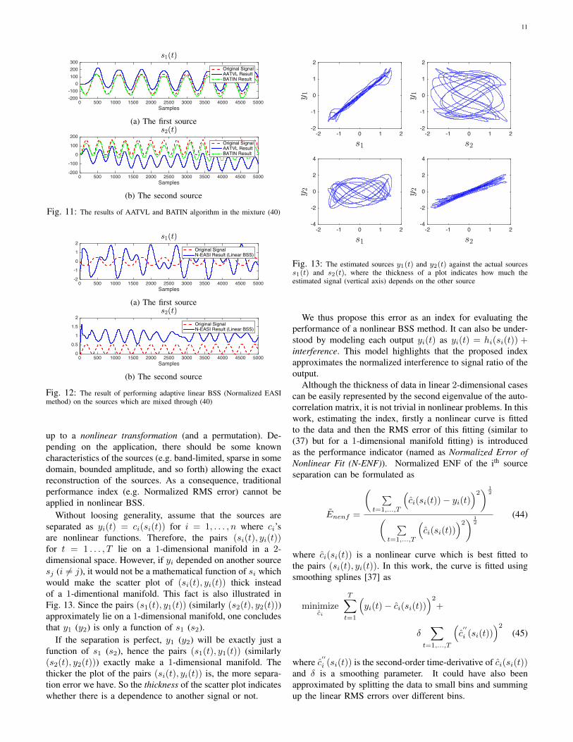
vations, we get the results shown in Fig. 10 for the firstsimulation (mapping of Eq. (2)), and Fig. 11 for the secondone (mapping of Eq. (40)). As expected, BATIN surpassesAATVL in estimating the separated sources in both simula-tions. Especially, the late convergence problem with AATVLhas been almost completely resolved by BATIN.

Additionally, in order to see that adaptive linear BSS algo-rithms are not able to separate the sources (since the mixtureis nonlinear), we have also implemented the same algorithmNormalized EASI for separating the mixture (40). It can beseen from Fig. 12 that the nonlinear mixture is not separatedat all since EASI never converges.

C. Performance EvaluationAs mentioned earlier in Section II-A, unlike linear BSS

where the sources may be estimated up to a scaling (anda permutation), in nonlinear problem, they can be estimated

11

Samples0 500 1000 1500 2000 2500 3000 3500 4000 4500 5000

-200-100

0100200300

s1(t)

Original SignalAATVL ResultBATIN Result

(a) The first source

Samples0 500 1000 1500 2000 2500 3000 3500 4000 4500 5000

-200

-100

0

100

200s2(t)

Original SignalAATVL ResultBATIN Result

(b) The second source

Fig. 11: The results of AATVL and BATIN algorithm in the mixture (40)

Samples0 500 1000 1500 2000 2500 3000 3500 4000 4500 5000

-2

-1

0

1

2s1(t)

Original SignalN-EASI Result (Linear BSS)

(a) The first source

Samples0 500 1000 1500 2000 2500 3000 3500 4000 4500 5000

0

0.5

1

1.5

2s2(t)

Original SignalN-EASI Result (Linear BSS)

(b) The second source

Fig. 12: The result of performing adaptive linear BSS (Normalized EASImethod) on the sources which are mixed through (40)

up to a nonlinear transformation (and a permutation). De-pending on the application, there should be some knowncharacteristics of the sources (e.g. band-limited, sparse in somedomain, bounded amplitude, and so forth) allowing the exactreconstruction of the sources. As a consequence, traditionalperformance index (e.g. Normalized RMS error) cannot beapplied in nonlinear BSS.

Without loosing generality, assume that the sources areseparated as y

i

(t) = c

i

(s

i

(t)) for i = 1, . . . , n where c

i

’sare nonlinear functions. Therefore, the pairs (s

i

(t), y

i

(t))

for t = 1 . . . , T lie on a 1-dimensional manifold in a 2-dimensional space. However, if y

i

depended on another sources

j

(i 6= j), it would not be a mathematical function of si

whichwould make the scatter plot of (s

i

(t), y

i

(t)) thick insteadof a 1-dimentional manifold. This fact is also illustrated inFig. 13. Since the pairs (s1(t), y1(t)) (similarly (s2(t), y2(t)))approximately lie on a 1-dimensional manifold, one concludesthat y1 (y2) is only a function of s1 (s2).

If the separation is perfect, y1 (y2) will be exactly just afunction of s1 (s2), hence the pairs (s1(t), y1(t)) (similarly(s2(t), y2(t))) exactly make a 1-dimensional manifold. Thethicker the plot of the pairs (s

i

(t), y

i

(t)) is, the more separa-tion error we have. So the thickness of the scatter plot indicateswhether there is a dependence to another signal or not.

-2 -1 0 1 2-2

-1

0

1

2

-2 -1 0 1 2-2

-1

0

1

2

-2 -1 0 1 2-4

-2

0

2

4

-2 -1 0 1 2-4

-2

0

2

4

Fig. 13: The estimated sources y1(t) and y2(t) against the actual sourcess1(t) and s2(t), where the thickness of a plot indicates how much theestimated signal (vertical axis) depends on the other source

We thus propose this error as an index for evaluating theperformance of a nonlinear BSS method. It can also be under-stood by modeling each output y

i

(t) as y

i

(t) = h

i

(s

i

(t)) +

interference. This model highlights that the proposed indexapproximates the normalized interference to signal ratio of theoutput.

Although the thickness of data in linear 2-dimensional casescan be easily represented by the second eigenvalue of the auto-correlation matrix, it is not trivial in nonlinear problems. In thiswork, estimating the index, firstly a nonlinear curve is fittedto the data and then the RMS error of this fitting (similar to(37) but for a 1-dimensional manifold fitting) is introducedas the performance indicator (named as Normalized Error ofNonlinear Fit (N-ENF)). Normalized ENF of the ith sourceseparation can be formulated as

˜

E

nenf

=

✓ Pt=1,...,T

⇣c

i

(s

i

(t))� y

i

(t)

⌘2◆ 1

2

✓ Pt=1,...,T

⇣c

i

(s

i

(t))

⌘2◆ 1

2

(44)

where c

i

(s

i

(t)) is a nonlinear curve which is best fitted tothe pairs (s

i

(t), y

i

(t)). In this work, the curve is fitted usingsmoothing splines [37] as

minimize

ci

TX

t=1

⇣y

i

(t)� c

i

(s

i

(t))

⌘2+

�

X

t=1,...,T

⇣c

00

i

(s

i

(t))

⌘2(45)

where c00

i

(s

i

(t)) is the second-order time-derivative of ci

(s

i

(t))

and � is a smoothing parameter. It could have also beenapproximated by splitting the data to small bins and summingup the linear RMS errors over different bins.

12

0 0.05 0.1 0.15 0.2 0.25 0.30

2

4

6

8 10-3

First SourceSecond Source

Fig. 14: The normalized ENF error in separating the mixture (2) for differentlevels of nonlinearity (represented by � in (39)) using BATIN algorithm

Simulation results of the algorithms are also compared interms of Normalized ENF error and can be found in table I.

TABLE I: N-ENF Error for AATVL and BATIN in thesimulations

AATVL BATIN

N-ENF for the Source 1 in the mixture (2) & (39) 0.0030 0.0019

N-ENF for the Source 2 in the mixture (2) & (39) 0.0084 0.0031

N-ENF for the Source 1 in the mixture (40) 0.0025 0.0023

N-ENF for the Source 2 in the mixture (40) 0.0064 0.0040

These results show that the proposed idea is able to sep-arate the sources that are mixed nonlinearly, which provesthe proposed concept. However, as mentioned earlier, theperformance of the proposed approach depends on the amountof the nonlinearity of the mixing function, i.e. as the mixingmodel gets distant from a linear mixture, the performance ofthe algorithm decreases. In order to show how the performancechanges according to the nonlinearity level, a 3

rd experimentis provided as follows.

Recall the example (2) with ↵(s(t)) defined as (39), letting↵0 = ⇡/6 and the parameter � vary. In this example, if � = 0,the mixture will be linear (a ⇡/6 rotation). But as � grows, themixture will become more nonlinear. Thus � can be consideredas a level of nonlinearity of this parametric model.

Finally, the algorithm BATIN is employed for separatingtwo sources of (41) and (42) mixed by (2), for different valuesof � in (39). The normalized ENF error of BATIN for bothsources is calculated and plotted in Fig. 14. Evidently, themore the mixture is nonlinear, the less efficient the proposedmethod is in separating the sources.

V. CONCLUSIONS AND PERSPECTIVES

In this paper, a novel approach for performing nonlinearBSS is proposed. Through this approach, it is shown thatthe nonlinear mixtures are generally separable under a fewassumptions (see subsection II-A). So the counter-examplesprovided in the literature to show that nonlinear mixtures arenot separable, are not valid any more.

The key idea is to regard the time-derivative of the observedsignals as a time-varying linear mixture of the (mutually in-dependent) time derivatives of the sources. As a consequence,

the model (6) will be obtained, where the mixing matrix is afunction of the sources (not to be confused with a time-variantmixing matrix which is a function of time).

Assuming both sources as functions of the time and non-linear mapping as a function of the sources to be smoothenough yields a sufficiently smooth mixing matrix which canbe considered as a time-variant model (AATVL algorithm).However, the model (6) being a function of sources instead ofconventional time-variant mixing models, enables performingthe nonlinear regression (as explained in Section III-C) anddramatically improves the performance of the separation,which resulted in proposing the second algorithm (BATIN).

Once the sources are separated, BSS has been performed.However, aiming at exactly estimating the sources (not onlyseparating them), the problem reduces to compensating anunknown nonlinear distortion. In other words, in order toprecisely estimating the source signals (compensating thenonlinear function), each of the separated signals should beconsidered separately.

Numerous algorithms have been proposed for blind restora-tion of nonlinearly distorted signals (e.g. [33], [32]). Theproposed methods are fundamentally based on retrieving somecharacteristics of the signal which are affected by nonlineardistortions. For example, nonlinear functions generally widenthe bandwidth of signals. Thus, given a distorted band-limitedsignal, one may recover the original signal by trying to min-imize its bandwidth via a nonlinear (compensating) function.

Moreover, assuming that the nonlinearly distorted signal issparse in some domain, it can be blindly reconstructed [39],[31]. Since nonlinear distortions generally tend to reduce thesparsity, the proposed algorithms compensate the distortion viaa sparse recovery procedure.

Nonetheless, depending on the application, there should besome known characteristics of the sources (e.g. band-limited,sparse in some domain, bounded amplitude, and so forth)allowing the exact reconstruction of the sources.

The basic idea proposed in this work is to utilize time-derivatives of the signals. Working with time-derivatives im-plicitly utilizes temporal information in the signals. Thisfact also supports the proposition in [27], which says thatalthough we may mix two sources so that the mixtures areinstantaneously independent of each other, it is highly probablethat their delayed versions are not mutually independent wheneach of them is temporally correlated. In other words, it isimplied in the paper that utilizing the temporal information ofthe sources may leads to solve nonlinear BSS problems.

It is worth noting that the proposed idea is quite differentwith respect to the previous works in the literature on nonlinearmixtures; it is more theoretic and general and does notassume any specific mixing model or source signals. Two basicmethods, AATVL and BATIN are provided in this work toshow how the idea is to be employed. Nevertheless, manydifferent separation algorithms can be suggested based on theproposed approach and they can be optimized to deal withmore complex signals/mixtures of practical applications.

13

However, there are several issues to be considered in thefuture. Firstly, the statistical characteristics of the derivativeof a signal with respect to those of the signal, itself, should beinvestigated. This might be the key to better understanding ofthe key feature of derivatives that lets perform the separation,and accordingly, it may lead to new algorithms of nonlinearBSS.

Secondly, the “Nonlinear Regression” used in the proposedalgorithm should be improved. The main objective of this stepis to accumulate the information of the separation at eachsample. For example, if at two different times, the sourcevector takes the same value, the mixing matrix will remainthe same as well.

The problem in this work is considered in the simplestform where there is no noise added to the signals. Since allthe signals in practical applications are noisy, and consideringthe fact that taking the derivatives may dramatically amplifiesthe noise, new methods should be developed which are morerobust to noise. It may also enforce some modifications on“Adaptive Linear BSS” procedure of the algorithms as well.

Last but not least, finding out the relations between autocor-relation functions of the sources (i.e. how much colored theyare) and the performance of the proposed approach and tryingto quantify it is also an interest for future studies.

REFERENCES

[1] J. Herault and C. Jutten, “Space or time adaptive signal processingby neural network models,” in AIP Conference Proceedings 151 onNeural Networks for Computing. Woodbury, NY, USA: AmericanInstitute of Physics Inc., 1987, pp. 206–211. [Online]. Available:http://dl.acm.org/citation.cfm?id=24140.24171

[2] P. Comon and C. Jutten, Handbook of Blind Source Separation: Inde-pendent component analysis and applications. Academic press, 2010.

[3] T. Mei, F. Yin, and J. Wang, “Blind source separation based oncumulants with time and frequency non-properties,” IEEE Transactionson Audio, Speech, and Language Processing, vol. 17, no. 6, pp. 1099–1108, 2009.

[4] P. Comon, “Independent component analysis, a new concept?” SignalProcessing, vol. 36, no. 3, pp. 287–314, 1994.

[5] A. J. Bell and T. J. Sejnowski, “An information-maximization approachto blind separation and blind deconvolution,” Neural computation, vol. 7,no. 6, pp. 1129–1159, 1995.

[6] J. F. Cardoso and A. Souloumiac, “An efficient technique for theblind separation of complex sources.” in Proceeding of IEEE SignalProcessing Workshop on Higher-Order Statistics, Lake Tahoe, 1993, pp.275–279.

[7] J. F. Cardoso and B. H. Laheld, “Equivariant adaptive source separation,”IEEE Transactions on Signal Processing, vol. 44, no. 12, pp. 3017–3030,1996.

[8] L. De Lathauwer, B. De Moor, and J. Vandewalle, “On the best rank-1and rank-(r 1, r 2,..., rn) approximation of higher-order tensors,” SIAMJournal on Matrix Analysis and Applications, vol. 21, no. 4, pp. 1324–1342, 2000.

[9] A. Hyvarinen, “Fast and robust fixed-point algorithms for independentcomponent analysis,” IEEE Transactions on Neural Networks, vol. 10,no. 3, pp. 626–634, 1999.

[10] L. Tong, V. C. Soon, Y. F. Huang, and R. Liu, “AMUSE: a new blindidentification algorithm,” in IEEE International Symposium on Circuitsand Systems, May 1990, pp. 1784–1787 vol.3.

[11] L. Tong, R. W. Liu, V. C. Soon, and Y. F. Huang, “Indeterminacy andidentifiability of blind identification,” IEEE Transactions on Circuits andSystems, vol. 38, no. 5, pp. 499–509, 1991.

[12] A. Belouchrani, K. Abed-Meraim, J.-F. Cardoso, and E. Moulines, “Ablind source separation technique using second-order statistics,” IEEETransactions on Signal Processing, vol. 45, no. 2, pp. 434–444, 1997.

[13] N. Dobigeon, J.-Y. Tourneret, C. Richard, J. C. M. Bermudez,S. McLaughlin, and A. O. Hero, “Nonlinear unmixing of hyperspectralimages: Models and algorithms,” IEEE Signal Processing Magazine,vol. 31, no. 1, pp. 82–94, 2014.

[14] M. Golbabaee, S. Arberet, and P. Vandergheynst, “Compressive sourceseparation: Theory and methods for hyperspectral imaging,” IEEETransactions on Image Processing, vol. 22, no. 12, pp. 5096–5110, 2013.

[15] I. Meganem, P. Deliot, X. Briottet, Y. Deville, and S. Hosseini, “Physicalmodelling and non-linear unmixing method for urban hyperspectralimages,” in Hyperspectral Image and Signal Processing: Evolution inRemote Sensing (WHISPERS), 3rd Workshop on. IEEE, 2011, pp. 1–4.

[16] L. T. Duarte and C. Jutten, “Design of smart ion-selective electrodearrays based on source separation through nonlinear independent compo-nent analysis,” Oil & Gas Science and Technology–Revue dIFP Energiesnouvelles, vol. 69, no. 2, pp. 293–306, 2014.

[17] F. Merrikh-Bayat, M. Babaie-Zadeh, and C. Jutten, “Linear-quadraticblind source separating structure for removing show-through in scanneddocuments,” International Journal on Document Analysis and Recogni-tion (IJDAR), vol. 14, no. 4, pp. 319–333, 2011.

[18] M. Babaie-Zadeh, “On blind source separation in convolutive andnonlinear mixtures,” Ph.D. dissertation, Grenoble, INPG, 2002.

[19] T. Blaschke, T. Zito, and L. Wiskott, “Independent slow feature analysisand nonlinear blind source separation,” Neural computation, vol. 19,no. 4, pp. 994–1021, 2007.

[20] D. N. Levin, “Performing nonlinear blind source separation with signalinvariants,” IEEE Transactions on Signal Processing, vol. 58, no. 4, pp.2131–2140, 2010.

[21] A. Taleb and C. Jutten, “Source separation in post-nonlinear mixtures,”IEEE Transactions on Signal Processing, vol. 47, no. 10, pp. 2807–2820,1999.

[22] Y. Altmann, A. Halimi, N. Dobigeon, and J. Y. Tourneret, “Supervisednonlinear spectral unmixing using a postnonlinear mixing model for hy-perspectral imagery,” IEEE Transactions on Image Processing, vol. 21,no. 6, pp. 3017–3025, 2012.

[23] A. Halimi, Y. Altmann, N. Dobigeon, and J. Y. Tourneret, “Nonlinearunmixing of hyperspectral images using a generalized bilinear model,”IEEE Transactions on Geoscience and Remote Sensing, vol. 49, no. 11,pp. 4153–4162, 2011.

[24] Y. Deville and L. T. Duarte, “An overview of blind source separationmethods for linear-quadratic and post-nonlinear mixtures,” in Interna-tional Conference on Latent Variable Analysis and Signal Separation.Springer, 2015, pp. 155–167.

[25] A. Hyvarinen and P. Pajunen, “Nonlinear independent component anal-ysis: Existence and uniqueness results,” Neural Networks, vol. 12, no. 3,pp. 429–439, 1999.

[26] A. M. Kagan, Y. V. Linnik, and C. R. Rao, “Extension of darmois-skitcvic theorem to functions of random variables satisfying an additiontheorem,” Communications in Statistics-Theory and Methods, vol. 1,no. 5, pp. 471–474, 1973.

[27] S. Hosseini and C. Jutten, “On the separability of nonlinear mixtures oftemporally correlated sources,” IEEE Signal Processing Letters, vol. 10,no. 2, pp. 43–46, 2003.

[28] C. Jutten and J. Karhunen, “Advances in nonlinear blind source separa-tion,” in Proceeding of the 4th International Symposium on IndependentComponent Analysis and Blind Signal Separation (ICA2003), 2003, pp.245–256.

[29] ——, “Advances in blind source separation (BSS) and independentcomponent analysis (ICA) for nonlinear mixtures,” International Journalof Neural Systems, vol. 14, no. 05, pp. 267–292, 2004.

[30] B. Ehsandoust, B. Rivet, C. Jutten, and M. Babaie-Zadeh, “Nonlinearblind source separation for sparse sources,” in 2016 24th EuropeanSignal Processing Conference (EUSIPCO), Aug 2016, pp. 1583–1587.

[31] L. T. Duarte, R. Suyama, R. Attux, J. M. T. Romano, and C. Jutten,“A sparsity-based method for blind compensation of a memoryless non-linear distortion: Application to ion-selective electrodes,” IEEE SensorsJournal, vol. 15, no. 4, pp. 2054–2061, 2015.

[32] K. Dogancay, “Blind compensation of nonlinear distortion for bandlim-ited signals,” IEEE Transactions on Circuits and Systems I: RegularPapers, vol. 52, no. 9, pp. 1872–1882, 2005.

[33] F. arvasti and A. K. Jain, “Zero crossings, bandwidth compression,and restoration of nonlinearly distorted band-limited signals,” Journalof Optical Society of America A, vol. 3, no. 5, pp. 651–654, May 1986.

[34] B. Ehsandoust, M. Babaie-Zadeh, and C. Jutten, Blind Source Separationin Nonlinear Mixture for Colored Sources Using Signal Derivatives.Springer International Publishing, 2015, pp. 193–200.

14

[35] M. Spivak, Calculus on Manifolds: A Modern Approach to ClassicalTheorems of Advanced Calculus, ser. Advanced book program. AvalonPublishing, 1965.

[36] J. B. Tenenbaum, V. d. Silva, and J. C. Langford, “A global geometricframework for nonlinear dimensionality reduction,” Science, vol. 290,no. 5500, pp. 2319–2323, 2000.

[37] C. H. Reinsch, “Smoothing by spline functions,” Numerische mathe-matik, vol. 10, no. 3, pp. 177–183, 1967.

[38] C. De Boor, A practical guide to splines. Springer-Verlag New York,1978, vol. 27.

[39] J. Malek, “Blind compensation of memoryless nonlinear distortionsin sparse signals,” in 21st European Signal Processing Conference(EUSIPCO 2013), Sept 2013, pp. 1–5.