the linear separability problem: some testing methods - sci2s

330 IEEE TRANSACTIONS ON NEURAL NETWORKS, VOL. 17, NO. 2, MARCH 2006

The Linear Separability Problem:Some Testing Methods

D. Elizondo

Abstract—The notion of linear separability is used widely in ma-chine learning research. Learning algorithms that use this conceptto learn include neural networks (single layer perceptron and re-cursive deterministic perceptron), and kernel machines (supportvector machines). This paper presents an overview of several ofthe methods for testing linear separability between two classes. Themethods are divided into four groups: Those based on linear pro-gramming, those based on computational geometry, one based onneural networks, and one based on quadratic programming. TheFisher linear discriminant method is also presented. A section onthe quantification of the complexity of classification problems is in-cluded.

Index Terms—Class of separability, computational geometry,convex hull, Fisher linear discriminant, linear programming,linear separability, quadratic programming, simplex, supportvector machine.

I. INTRODUCTION

TWO SUBSETS and of are said to be linearlyseparable (LS) if there exists a hyperplane of such

that the elements of and those of lie on opposite sides of it.Fig. 1 shows an example of LS and NLS set of points. Squaresand circles denote the two classes.

Linear separability is an important topic in the domain ofmachine learning and cognitive psychology. A linear model israther robust against noise and most likely will not over fit. Mul-tilayer non linear neural networks, such as the back propagationalgorithm, work well for classification problems. However, asthe experience of perceptrons has shown, there are many real lifeproblems in which there is a linear separation. For such prob-lems, using backpropagation is an overkill, with thousands ofiterations needed to get to the point where linear separation canbring us fast. Furthermore, multilayer linear neural networks,such as the recursive deterministic perceptron (RDP) [1], [2]can always linearly separate, in a deterministic way, two or moreclasses (even if the two classes are not linearly separable). Theidea behind the construction of an RDP is to augment the affinedimension of the input vector by adding to these vectors the out-puts of a sequence of intermediate neurons as new components.Each intermediate neuron corresponds to a single layer percep-tron and it is characterized by a hyperplane which linearly sep-arates an LS subset, taken from the non-LS (NLS) original set,

Manuscript received July 24, 2003; revised June 15, 2005.The author is with the Centre for Computational Intelligence, School of Com-

puting, De Montfort University, The Gateway, Leicester LEI 9BH, U.K. (e-mail:[email protected]).

Digital Object Identifier 10.1109/TNN.2005.860871

Fig. 1. (a) LS set of points. (b) Non-LS set of points.

and the remaining points in the input vector. A cognitive psy-chology study on the subject of linear separability constraint oncategory learning is presented in [3]. The authors stress the factthat grouping objects into categories on the basis of their sim-ilarity is a primary cognitive task. To the extent that categoriesare not linearly separable, on the basis of some combination ofperceptual information, they might be expected to be harder tolearn. Their work tries to address the issue of whether categoriesthat are not linearly separable can ever be learned.

Linear separability methods are also used for training supportvector machines (SVM) used for pattern recognition [4], [5].Similar to the RDP, SVMs are linear learning machines on LS

1045-9227/$20.00 © 2006 IEEE

ELIZONDO: THE LINEAR SEPARABILITY PROBLEM: SOME TESTING METHODS 331

and NLS data. They are trained by finding a hyperplane thatlinearly separates the data. In the case of NLS data, the data ismapped into some other Euclidean space. Thus, SVM is stilldoing a linear separation but in a different space.

This paper presents an overview of several of the methods fortesting linear separability between two classes. In order to dothis, the paper is divided into five sections. In Section II, somestandard notations and definitions together with some generalproperties related to them are given. In Section III, some of themethods for testing linear separability, and the computationalcomplexity for some of them are provided. These methods in-clude those based on linear programming, computational geom-etry, neural networks, quadratic programming, and the Fisherlinear discriminant method. Section IV deals with the quan-tification of the complexity of classification problems. Finally,some conclusions are pointed out in Section V.

II. PRELIMINARIES

The following standard notions are used: LetCard stands for the cardinality of a set . is the

set of elements which belongs to and does not belong to .is the set of elements of the form with and

. stands for , i.e., the set of elements ofthe form with and . Ifand , then corresponds to

. Letbe the standard position vectors representing two points and

in ; the set is called the seg-ment between and is denoted by . The dot productof two vectors is definedas .and by extension .stands for the hyperplane of ofthe normal , and the threshold . will stand for the set of allhyperplanes of .

The fact that two subsets and of are lin-early separable is denoted by or . Thus,if , then and

or and. Let

. Letbe the half space delimited by and containing (i.e.,

if for some.

A. Definitions and Properties

For the theoretical representations, column vectors are usedto represent points. However, for reasons of saving space, whereconcrete examples are given, row vectors are used to representpoints. We also introduce the notions of convex hull and linearseparability.

Definition 2.1: A subset of is said to be convex if, forany two points and in , the segment is entirelycontained in .

Fig. 2. Convex hull of a set of six points.

Fig. 3. (a) Affinely independent and (b) dependent set of points.

Definition 2.2: Let be a subset of , then the convex hullof , denoted by , is the smallest convex subset ofcontaining .

Property 2.1: [6]: Let be a subset of .

•and .

• If is finite, then there exists andsuch that

for . Thus, is the intersection of halfspaces.

Fig. 2 represents the convex hull for a set of six points with avalue of .

Property 2.2: If and then.

Definition 2.3: Let be a subset of points in and let; then (dimension affine) is the dimension of

the vectorial subspace generated by .In other words, is the dimension of the smallest

affine subspace that contains . does not depend onthe choice of .

Definition 2.4: A set of points is said to be affinely inde-pendent if Card .

In other words, given points in , they are

said to be affinely independent if the vectors

are linearly independent. In an affinely dependentset of points, a point can always be expressed as a linear combi-nation of the other points. Fig. 3 shows an example of an affinelyindependent and dependent set of points with coefficients sum-ming to 1.

Property 2.3: If , then .In other words, if we have a set of points in dimension , the

maximum number of affinely independent points that we canhave is . There are no affinely independent points;


so if we have for example 25 points in , these points arenecessarily affinely dependent. If not all the points were placedin a straight line, we could find three points which are affinelyindependent.

III. METHODS FOR TESTING LINEAR SEPARABILITY

In this section we present some of the methods for testinglinear separability between two sets of points and . Thesemethods can be classified in five groups

1 ) methods based on linear programming;2 ) methods based on computational geometry;3 ) method based on neural networks;4 ) method based on quadratic programming;5 ) Fisher linear discriminant method.

A. Methods Based on Linear Programming

In these methods, the problem of linear separability is repre-sented as a system of linear equations. If two classes are LS, themethods find a solution to the set of linear equations. This so-lution represents the hyperplane that linearly separates the twoclasses.

Several methods for solving linear programming problemsexist. Two of the most popular ones are the Fourier–Kuhn elim-ination and the Simplex Method [7]–[10].

1) The Fourier–Kuhn Elimination Method: This methodprovides a way to eliminate variables from a set of linearequations. To demonstrate how the Fourier–Kuhn eliminationmethod works, we will apply it to both the AND and the XORlogic problems.

a) The AND Problem: Let andrepresent the input patterns for

the two classes which define the AND problem. We want tofind out if .

Let

By doing the above, a mapping of the two-dimensional (2-D)LS problem into a three-dimensional (3-D) LS problem is ob-tained where the separating plane passes through the origen.This mapping is done throughout the paper.

Thus, to find out if , we need to find a set of values forthe weights , and threshold such that

The method consists of eliminating every time a variable from aset of inequalities. To do so, we consider all pairs of inequalitiesin which a variable has opposite signs, and eliminate it betweeneach pair. Thus, if we choose to eliminate (positive in , andnegative in the rest of the equations) we have

Since at this step all the variables have the same sign (they areall positive), we want to know if this new system of equationsadmits a solution which satisfies

and and

We can confirm that a set of values satisfying these constraintsis: , and . Thus, we have proven that

.b) The XOR Problem: Let and

represent the input patterns for the two classeswhich define the XOR problem. We want to find out if .

Let . We now have. Thus, to

find out if , we need to find a set of values for the weights, and threshold such that

As in the AND example, we choose to eliminate (positive inand , and negative in the rest of the equations). This produces

At this point, we observe that inequalities 1 and 4 (2 and3) contain a contradiction. Therefore, we conclude that theproblem is infeasible, and that .

c) Complexity: This method is computationally imprac-tical for large problems because of the large build-up in inequali-ties (or variables) as variables (or constraints) are eliminated. Itscomputational complexity is exponential and can result in theworst case in constraints (for inequalities involving

variables).2) The Simplex Method: The Simplex method is one of the

most popular methods used for solving linear programs. A linearprogram can be seen as a set of variables which are contained ina linear expression called the objective function. The goal is tofind values to these variables which maximize or minimize theobjective function subject to constraints. These constraints oflinear expressions must be either or to a given value.There are three possible results when trying to solve a linearprogram.

1) The model is solvable. This means that there exists a setof values for the variables that provide an optimal valueto the objective function.

2) The model is infeasible. This means that there are novalues for the variables which can satisfy all the con-straints at the same time.

3) The model is unbounded. This means that the value ofthe objective function can be increased with no limit bychoosing values to the variables.

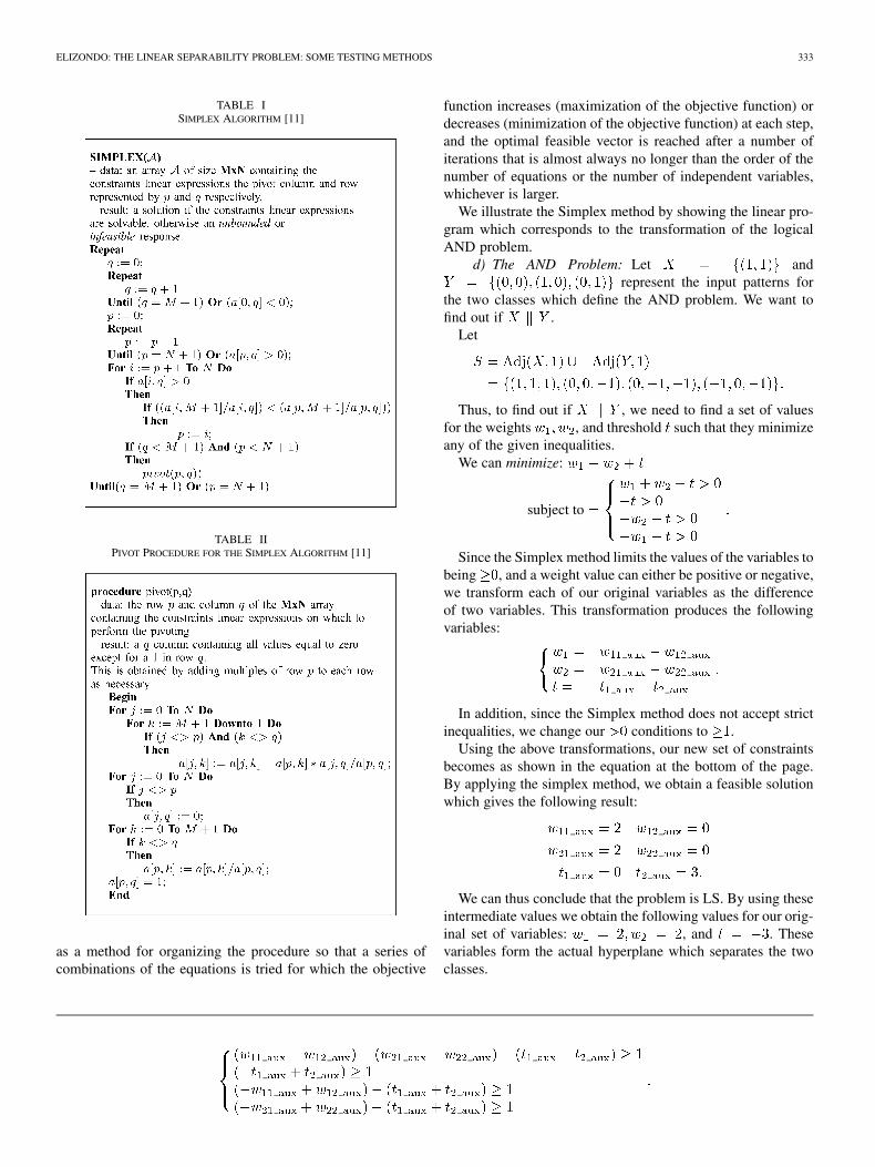
In this paper, we use the Simplex algorithm for testing linearseparability among two classes. The algorithms in Tables Iand II show the Simplex procedure. This algorithm consists offinding the values of and to pivot and repeating the processuntil either an optimum value is obtained, or the linear programis determined to be infeasible. This method can be viewed


TABLE ISIMPLEX ALGORITHM [11]

TABLE IIPIVOT PROCEDURE FOR THE SIMPLEX ALGORITHM [11]

as a method for organizing the procedure so that a series ofcombinations of the equations is tried for which the objective

function increases (maximization of the objective function) ordecreases (minimization of the objective function) at each step,and the optimal feasible vector is reached after a number ofiterations that is almost always no longer than the order of thenumber of equations or the number of independent variables,whichever is larger.

We illustrate the Simplex method by showing the linear pro-gram which corresponds to the transformation of the logicalAND problem.

d) The AND Problem: Let andrepresent the input patterns for

the two classes which define the AND problem. We want tofind out if .

Let

Thus, to find out if , we need to find a set of valuesfor the weights , and threshold such that they minimizeany of the given inequalities.

We can minimize:

subject to

Since the Simplex method limits the values of the variables tobeing , and a weight value can either be positive or negative,we transform each of our original variables as the differenceof two variables. This transformation produces the followingvariables:

In addition, since the Simplex method does not accept strictinequalities, we change our conditions to .

Using the above transformations, our new set of constraintsbecomes as shown in the equation at the bottom of the page.By applying the simplex method, we obtain a feasible solutionwhich gives the following result:

We can thus conclude that the problem is LS. By using theseintermediate values we obtain the following values for our orig-inal set of variables: , and . Thesevariables form the actual hyperplane which separates the twoclasses.


Fig. 4. Convex hulls for (a) LS and (b) non-LS set of points.

e) Complexity: One of the problems that the SimplexMethod presents is that there is no known best strategy forselecting the pivot element because there are no results to tellus how many pivot steps to expect for any reasonable sizeproblem.

The complexity of this method depends on the pivot rule used.A description of apparently all currently known bad examplesfor various pivot rules in a uniform way can be found in [12].These rules include

• greatest increase rule;• Dantzig(c)s largest coefficient rule;• Bland(c)s least index rule;• Gass-Saaty shadow vertex rule.

The largest number of vertices, and therefore, the maximalnumber of steps of the simplex algorithm with the worst pos-sible pivot sequence on a linear programming problem in fixeddimensions, and containing facets, is equal to ).

B. The Methods Based on ComputationalGeometry Techniques

In this section, we discuss two methods for testing linear sep-arability that are based on computational geometry techniques[13].

1) The Convex Hull Method for Testing Linear Separa-bility: The following method makes use of the notion ofconvex hull. Two classes and are LS if the intersectionof the convex hulls of and is empty. Fig. 4 presents theconvex hulls for an LS set of points, with an empty intersection,and an NLS set of points, with a nonempty intersection.

Lemma 3.1: Let.

Lemma 3.2: Let thenand . Thus,

.Lemma 3.3: Let be two finite subsets of

.Theorem 3.1: Let be two finite subsets of , then

iff .Property 3.1: Let be a finite subset of , then there exists

such that .

TABLE IIICONVEX HULL SEPARABILITY ALGORITHM

This property states that there exists a point which isLS from the rest of the points in .

Remark: The Lemmas 3.1, 3.2, and 3.3 and the Property 3.1are intuitively evident and their proofs are not relevant for theglobal comprehension of this work. Formal proofs can be foundin [2]. A more general result than the one shown in Theorem 3.1can be found in [14].

Property 3.2: Let be a finite subset of , and assumethat We have the following:

• if for all , then ;• if there exists such that , then ,

where , and.

Proof:

• If for all , then and; thus, by the Theorem 3.1, we conclude that

.• If there exists such that then, for every and

we have , that is .Let , and

. It is clear that , and therefore

We conclude that .The convex hull separability algorithm presented in Table III

is based in this property. Given , this algorithmcomputes and (if they exist) such that

, where and represent the weight vector andthreshold value which make the hyperplane that linearly sep-arates and .

Following Property 3.2, the convex hullis obtained as the set of points which verify the constraints

, where is the numberof vertices in the convex hull. This algorithm is applied in twosteps.


Fig. 5. XY PLOT of the 2-D classification problem.

1 ) If for all , then the two classes are NLS.2 ) If there exists such that , then the two classes are

LS: With this value of we compute the values of andwhich correspond respectively to the maximum value of

the vector product of with belonging to the finite setof points of the second class , and the minimum valueof the vector product of with belonging to the finiteset of points of the first class . These two values are thenused to compute the threshold value which is definedby . The set of weights that represents thehyperplane that linearly separates the two classes and

, corresponds to .We will use the two-class, two-dimensional classification

problem shown in Fig. 5 to illustrate the Convex Hull separa-bility algorithm.

Let andrepresent the input patterns for the

two classes which define these classification problem. We wantto find out if .

We calculate

We then compute the convex hull of

Thus, we now know that ( represents the number ofvertices in the CH). Next, we compute all the vectors whichare perpendicular to each of the facets that form the CH togetherwith the corresponding values of (see Fig. 6).

Fig. 6. Convex Hull of X Y for the 2-D classification problem.

We can now select any of the pairs having a value. In our example, we have two choices for the value

and 6. Taking, we have the following values of and :

We can now compute the values of and

These weight vector and threshold values produce

Input P. NetInput

NetOutput Class

Fig. 7 shows the hyperplane which linearly separates the twoclasses and . Enclosed in a circle are the three points whichrepresent and , the two values used to calculate the thresholdvalue .

There are other methods based on computational geometrythat can be found in the literature for testing linear separability.Examples of this are the open hemisphere method [15], and therotating calipers algorithm [16].

f) Complexity: A common algorithm used for computingconvex hulls is the Quick-hull. The complexity of this algorithmis of for the average case, and of for the worstcase with an overall complexity similar to that of the Quick sort


Fig. 7. Hyperplane that linearly separates the 2-D classification problem(dotted line).

TABLE IVCLASS OF LINEAR SEPARABILITY METHOD

algorithm (these complexities are for the case of two dimen-sions). An in depth article concerning the complexity of dif-ferent algorithms for computing the convex hull can be foundin [17].

2) The Class of Linear Separability Method: In this section,we characterize the set of points of by which passes a hyper-plane that linearly separates two given LS classes. This charac-terization is going to allow us to infer the algorithm for testinglinear separability described in Table IV.

g) Characterization of the Class of Linear Separa-bility: Let and be two finite and disjoint subsets of

, and let be the set of points by which passesa hyperplane that linearly separates and . Clearly,

.Before characterizing the set , we give the following

result which presents the linear separability property as a localproperty.

Proposition 3.1: Let and be subsets of points of ,then and are linearly separable if and only if for everysubset containing at most points,and are linearly separable.

After giving some specific notations, we will characterize theset .

Property 3.3: Let be finite subsets of such that, and let . Then,

with, and and are sets which are closed,

unbounded, and convex. is called a linear separabilityclass of relatively to . In other words, if we have the classof separabilities between two LS classes, we can take a point thatdoes not belong to either of the two classes of separability, andwe can always find a hyperplane that passes through this pointand linearly separates the two classes. We characterize here allthe points by which pass all the hyperplanes that linearly sepa-rate the two LS classes.

Proof: Let , and note

then and are convex becauseand are convex.

Moreover, if then suchthat . Let because

, hence, thus is a closed set in . Let

and and consider the straight linedefined by .

Assume that is bounded, then there existssuch that for all . Let ,then because . Then,there exists such that and

. Thus, . Then, thereexists such that ; hence,

which is absurd, thus .Property 3.4: Let then ; if there

exists such thatand

or and.

Proof:

1) Assume that there exists such that

andand assume that

and .Let ;and .Let and .Then, by construction .

2) Assume that and assume by induc-tion that there exists such that

and. Let

and . An orthog-onal family (i.e., is an orthogonalbasis of such that

and.

Two vectors and areorthogonal if .

Assume that and letbe the continuous functions such that


Fig. 8. Example of a class of linear separability.

for .Then, , if

, then. Let

andthen and

,because

and .Hence,

or and.

h) Class of Linear Separability Method: Let be a hy-perplane of . is the half of delimitedby and containing . We assume that all points of are inthe same size of . Given , the class of linearseparability procedure, presented in the algorithm IV, computesrecursively and . (if there exists) such that

.Property 3.5: Let , such that

then, where

Cardis a set of affinely independent

points and

ifif

where is a hyperplancecontaining

The proof of the this property can be found in [2].Fig. 8 presents an example of a class of linear separability.

In this figure, we have two classes and having some hypo-thetical values and . We then have that

represents the linear separability class of class withrespect to class (black area), and the linear separa-bility class of class with respect to class (gray area).

To demonstrate how the class of linear separa-bility method works, we will apply it to a two-class,two-dimensional classification problem. Let

andrepresent the input patterns for the two classes which defineour problem. We want to find out if . Fig. 9(a) shows aplot of the two classes. Following the algorithm, we want toidentify all the hyperplanes with the following characteristics:

1 ) pass by one point of each of the two classes;2 ) linearly separate the remaining points.In this example, there is only one such hyperplane as

illustrated in Fig. 9(b). This hyperplane is represented by. We now recursively reduce the original dimen-

sion of the problem to one dimension so as to locate all thepoints, by which the selected hyperplane passes in one line.Once this is done, we calculate the middle point between thetwo original points belonging to each of the classes. Next, wecalculate a hyperplane in the original dimension that passesby this middle point and is different than the first hyperplane.This is illustrated in Fig. 9(c). The selected two points arehighlighted with a circle ( and ). They correspond to thepoints (4,5), and (5,4) respectively. Thus the middle point hasa value equal to 4.5. This second hyperplane is represented by

. With these two hyperplanes we now computethe values of and in the following way:

where and correspond to the set of points by which thefirst hyperplane does not pass as illustrated in Fig. 9(d). We usethese values for and to calculate the final hyperplane whichlinearly separates the two classes in the following way:


Fig. 9. Steps followed by the class of linear separability for finding the hyperplane which linearly separates classes X and �.

This is illustrated in Fig. 9(e). The final hyperplaneis represented by a dotted line and corresponds to

. This final hyperplane is illustrated inFig. 9(f).

i) Complexity: This algorithm transforms recursively theproblem of linear separability from dimensions to . Thistransformation may require operations in the worse case.Thus, in order to simplify the search of this hyperplane, any hy-perplane can be used to begin with, which can be moved in func-tion of the points until it contains a set of affinely independent

points of the two classes, and that linearly separates the rest ofthe points.

C. The Methods Based on Neural Networks

1) The Perceptron Neural Network: The first neural networkapplied to the problem of separating patterns into two categorieswas proposed by McCulloch and Pitts [18]. This network com-putes the weighted sum of the input patterns and compares it toa threshold value . If the net input is greater than the threshold,


TABLE VPERCEPTRON LEARNING ALGORITHM

Fig. 10. Perception for a 2-D classification problem.

the output of the network is ; otherwise, the output value is. This network is represented as follows:

NetInput

NetOutputif NetInput Thresholdif NetInput Threshold

where and correspond to the weightand input vector. The threshold value represents the minimalactivity needed for the network to produce a positive output.Rosenblatt [19] transformed this algorithm into the first train-able neural network which he called the perceptron. Table Vshows the pseudocode for the perceptron procedure.

Fig. 10 shows a perceptron network for a two-dimensionalclassification problem. We can take, as an example to illustratethe perceptron algorithm, the binary function AND.

Let andrepresent the input patterns for the two classes,and , which define the AND problem. We want tofind a weight vector and a threshold such that

. We note, from previous calculations,,

and.

Following the algorithm V, we have

TABLE VIALPHA VALUES FOR THE QP SOLUTION TO THE 2-D CLASSIFICATION PROBLEM

Thus, . In other words, a set of values forthe weight vector and the threshold that linearly separatesthe two classes and are: , and ,respectively. These weight vector and threshold values produce

InputPattern NetInput NetOutput Class

j) Complexity: A complexity analysis of the percep-tron algorithm can be found in [20]. The authors show thateach iteration of the perceptron algorithm takes time.Furthermore, under a Gaussian perturbation of variancewhere d, the perceptron algorithm converges in

iterations (if the problem isLS).

A geometry-based convergence upper bound for the percep-tron learning algorithm is presented in [2]. This upper bound isbased on the method described above for testing linear separa-bility based on convex hulls.

D. Methods Based on Quadratic Programming

The training procedure for these methods consists in solvinga quadratic programming optimization problem (QPOP). Thisis the case for the support vector machines (SVM). The SVM[21], [22] are linear learning machines that can be applied toclassification problems involving both LS and NLS data sets[23], [24]. They can find a hyperplane that linearly separatesa data set by solving a constrained QPOP.

In the case of NLS data, the data is mapped into some otherEuclidean space; so that the SVM is still doing a linear separa-tion but in a different space.

An on hands tutorial into classification using SVM can befound in [25]. The hyperplane separating two classes is definedas

where corresponds to slack variables in optimization theoryand , if the there is no error for (they will all be zeroif the two classes are LS).


TABLE VIIPRODUCT OF THE DECISION REGION AND CLASS ASSIGNATION FOR EACH DATA POINT

For a training data set with input vectorand output value the SVM needs to find a solu-tion to the optimization problem

Minimize

subject to

where represents the penalty parameter between the errorterm and the margin of the hyperplane.

We can represent this problem in its dual form as

Maximize

subject to

A kernel function must be used on the SVM. In its simplestform, a kernel function calculates the dot product of two trainingvectors. This helps with the evaluation of the correct classifica-tion of each training vector. Some of the most common kernelsused include

• linear: ;• polynomial: ;• radial basis function:

;• sigmoid: ;

where , and are kernel parameters.To illustrate how the SVM works, we will apply it to the fol-

lowing 2-D LS set of input vectors:

Class 1

Class 2

which represent the input vector for the two LS classes. Let

represent the output value (-1 Class 1, and 1 Class 2). We wantto find out if Class 1 Class 2.

To solve this problem we need to solve the following opti-mization problem:

Maximize

subject to

This allows to find the Lagrange multipliers associated withthe classification constrains.

Table VI shows the resulting values of obtained by usinga QP solver. The support vectors are the vectors with .

We can now use the Lagrange multipliers to obtain the valueof the hyperplane that linearly separates the two classes

The value of (the bias) can be obtained by

If we choose , then we obtain . Using these twovalues, our decision boundary becomes

for class 1

for class 2

Table VII shows the output values obtained by applying thedecision boundary to the classification points.

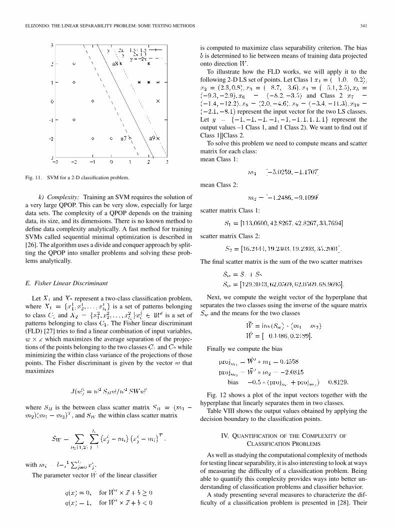
Fig. 11 shows a plot of the input vectors together with the hy-perplane that linearly separates them in two classes. The supportvectors , and are also displayed.


Fig. 11. SVM for a 2-D classification problem.

k) Complexity: Training an SVM requires the solution ofa very large QPOP. This can be very slow, especially for largedata sets. The complexity of a QPOP depends on the trainingdata, its size, and its dimensions. There is no known method todefine data complexity analytically. A fast method for trainingSVMs called sequential minimal optimization is described in[26]. The algorithm uses a divide and conquer approach by split-ting the QPOP into smaller problems and solving these prob-lems analytically.

E. Fisher Linear Discriminant

Let and represent a two-class classification problem,where is a set of patterns belongingto class and is a set ofpatterns belonging to class . The Fisher linear discriminant(FLD) [27] tries to find a linear combination of input variables,

which maximizes the average separation of the projec-tions of the points belonging to the two classes and whileminimizing the within class variance of the projections of thosepoints. The Fisher discriminant is given by the vector thatmaximizes

where is the between class scatter matrix, and the within class scatter matrix

with

The parameter vector of the linear classifier

for

for

is computed to maximize class separability criterion. The biasis determined to lie between means of training data projected

onto direction .To illustrate how the FLD works, we will apply it to the

following 2-D LS set of points. Let Class 1

and Class 2

represent the input vector for the two LS classes.Let represent theoutput values –1 Class 1, and 1 Class 2). We want to find out ifClass 1 Class 2.

To solve this problem we need to compute means and scattermatrix for each class:mean Class 1:

mean Class 2:

scatter matrix Class 1:

scatter matrix Class 2:

The final scatter matrix is the sum of the two scatter matrixes

Next, we compute the weight vector of the hyperplane thatseparates the two classes using the inverse of the square matrix

and the means for the two classes

Finally we compute the bias

bias

Fig. 12 shows a plot of the input vectors together with thehyperplane that linearly separates them in two classes.

Table VIII shows the output values obtained by applying thedecision boundary to the classification points.

IV. QUANTIFICATION OF THE COMPLEXITY OF

CLASSIFICATION PROBLEMS

As well as studying the computational complexity of methodsfor testing linear separability, it is also interesting to look at waysof measuring the difficulty of a classification problem. Beingable to quantify this complexity provides ways into better un-derstanding of classification problems and classifier behavior.

A study presenting several measures to characterize the dif-ficulty of a classification problem is presented in [28]. Their


Fig. 12. Hyperplane for a 2-D classification problem using Fisher linear discriminant.

TABLE VIIIPRODUCT OF THE DECISION REGION AND CLASS ASSIGNATION FOR EACH DATA POINT

study focuses in the geometrical characteristics of the class dis-tributions. The authors analyze measures that can emphasizethe way in which classes are separated or interleaved, whichplay a role in the level of accuracy of classification. These mea-sures include: overlap of individual feature values; separabilityof classes; and geometry, topology, and density of manifolds.

Another study on the measurement of the classifiability of in-stances of classification problems is presented in [29]. For thispurpose, the authors propose a nonparametric method based onthe evaluation of the texture of the class label surface. When theinstances of a class are interlaced with another class, the sur-face is rough. The surface is smoother when the class regionsare compact and disjoint. The texture of the class label surface

is characterized by the use of a co-ocurrence matrix. They applythis approach to a look-ahead-based fuzzy decision tree induc-tion that splits the instances of a particular node in such a way asto maximize the number of correct classifications at that node.

These characterization approaches can be used as another cri-teria from which to select the most adequate classifier for a spe-cific problem.

V. DISCUSSION AND CONCLUDING REMARKS

Several of the existing methods for testing linear separabilitybetween two sets of points and the complexities associated with


TABLE IXSUMMARY OF THE COMPUTATIONAL COMPLEXITIES OF SOME OF THE

METHODS FOR TESTING LINEAR SEPARABILITY

some of the algorithms have been presented. The methods pre-sented have been divided into four groups.

• The methods based on solving systems of linear equations.These methods include: the Fourier–Kuhn elimination al-gorithm, and the Simplex algorithm. The original classifi-cation problem is represented as a set of constrained linearequations. If the two classes are LS, the two algorithmsprovide a solution to these equations.

• The methods based on computational geometry tech-niques. We focused on the convex hull algorithm and theclass of linear separability method. If two classes are LS,the intersection of the convex hulls of the set of pointsthat represent the two classes is empty. The class of linearseparability method consists in characterizing the set ofpoints of by which it passes a hyperplane thatlinearly separates two sets of points and .

• The methods based on neural networks. The method de-scribed in this section is the perceptron learning algorithm.If the two classes are LS, the perceptron algorithm is guar-anteed to converge, after a finite number of steps, and willfind a hyperplane that separates them.

• The methods based on quadratic programming. Thesemethods can find a hyperplane that linearly separates twoclasses by solving a quadratic optimization problem. Thisis the case for the SVM.

• The Fisher linear discriminant method. This method triesto find a linear combination of input variables,which maximizes the average separation of the projectionsof the points belonging to the two classes and whileminimizing the within class variance of the projections ofthose points.

Table IX presents a summary of the complexities of some ofthe algorithms for testing linear separability described in thispaper.

Other methods for testing linear separability include theTarski elimination algorithm [30] which verifies the validity ofa special first order formula in an algebraic closed field

It is well known that the first-order logic for an algebraicclosed field is decidable.

Several aspects should be considered when choosing amethod for testing linear separability for a given problem.Some of these aspects include: the complexity level, thedifficulty of the classification problem, the easiness of imple-mentation, and the degree of linear separability that can beobtained when dealing with nonlinearly separable sets.

The Fourier-Khun elimination method is computationally im-practical for large problems due to the large build-up in inequali-ties (or variables) as variables (or constraints) are eliminated. Itscomputational complexity is exponential and can result in theworst case in constraints (for inequalities involving

variables).From a complexity point of view, the simplex method is re-

markably efficient in practice and is guaranteed to find the globaloptimum. However, in some cases, this method has markedlyvarying response times. Most of the times it is extremely fast,but when a succession of pivots are required, it slows down con-siderably, given rise to a less stable iteration.

The linear separability algorithm based on the convex hull ofthe data sets is simple to implement in three or less dimensions.It becomes more difficult as the dimension of the problem aug-ments. It is important to use effective storage techniques andtake into account possible imprecision in measurement. Onemust decide how to store a convex hull, once found, which isespecially tricky to do in higher dimensions. Hulls are gener-ally stored as a list of the highest dimensional facets (facets intwo dimensions), the neighboring facets for each facet, as wellas the vertices associated with the facets. This allows for a wayto add extra points to a computed hull.

The class of linear separability method can have a high com-putational complexity. However, this method cannot only beused for testing linear separability, but also for finding linearlyseparable subsets of maximum cardinality from within a nonlin-early separable set of points [31]. The concept of linearly sep-arable subsets of maximum cardinality is used as the basis forconstructing RDP multilayer linear networks.

From an implementation point of view, the perceptron neuralnetwork is probably one of the simplest algorithm to program.However, this algorithm is not very stable. There is also no wayto know after how many weight updates one can conclude that ifthe algorithm has not converged, the problem at hand is not lin-early separable. A convergence upper bound for this algorithmhas been developed by Elizondo [2]. This bound remains hardto compute, and further work needs to be done before it couldbe of practical use.

The SVM method is an efficient learning algorithm. Some ofits advantages include its ability to handle nonlinear classifica-tion problems that are nonseparable using linear methods; thehandling of arbitrary complex classifications, and the flexibilityand avoidance of overfitting. A key issue with this method isfinding the right kernel that will map a nonlinearly separabledata set into a higher dimension making it linearly separable.Training an SVM involves finding a solution to a very largeQPOP. This can prove very slow for large data sets. The sequen-tial minimal optimization method is a fast method for trainingSVMs. It uses a divide and conquer approach to minimize thetraining time.

The Fisher linear discriminant is a well-known method fortesting linear separability. The method has proven very powerfuland popular among users of discriminant analysis. Some rea-sons for this are its simplicity and unnecessity of strict assump-tions. However, this method has optimality properties only if theunderlying distributions of the groups are multivariate normal.The discriminant rule obtained can be seriously harmed by only


a small number of outlying observations. Outliers are hard todetect in multivariate data sets. The method is not very robustbecause it uses the sample means and variances, which can beaffected by one sufficiently large point. Kernel variations of thismethod have been proposed that can be used for nonlinear pat-tern recognition.

All the methods above will provide a hyperplane only if thetwo classes are linear separable. Both the SVM and the Fisherlinear discriminant will provide a hyperplane even if the twoclasses are nonlinearly separable.

Future directions in the area of linear separability includethe optimization of the hyperplanes that linearly separate twoclasses in order to maximize the generalization level. In otherwords, once we know that two classes are linearly separable,there exists an infinite number of hyperplanes that can separatethem linearly. How does one select the hyperplane that providesthe highest level of generalization? This will involve a deepcomparison study of the levels of generalization obtained withthe different methods for testing linear separability, involvingseveral real world data sets and benchmarks. Another interestingaspect to study is to include linear separability probabilities.This will make a set of points linearly separable within a cer-tain probability making the decision regions less rigid. Most re-search involving linear separability has been conducted usingtasks that involve learning two classes with a small number ofdata samples. It could be useful to do more research involvinglinear separability for more than two classes and larger data sets.

ACKNOWLEDGMENT

The author would like to thank the Associate Editor and twoanonymous referees for all their detailed comments and sug-gestions that have clearly improved the final presentation of thispaper. He would also like to thank especially to Dr. R. John,Dr. F. Chiclana, and R. Birkenhead from the CCI group at theSchool of Computing of De Montfort University for their feed-back on this paper.

REFERENCES

[1] M. Tajine and D. Elizondo, “Enhancing the Perceptron Neural Networkby Using Functional Composition,” Comp. Sci. Dept., Univ. Louis Pas-teur, Strasbourg, France, Tech. Rep. 96-07, 1996.

[2] D. A. Elizondo, “The Recursive Determinist Perceptron (rdp) andTopology Reduction Strategies for Neural Networks,” Ph.D. disserta-tion, Univ. Louis Pasteur, Strasbourg, France, Jan. 1997.

[3] M. Blair and D. Homa, “Expanding the search for a linear separabilityconstraint on category learning,” Memory and Cognition, vol. 29, no. 8,pp. 1153–1164, 2001.

[4] N. Cristianini and J. Shawe-Taylor, An Introduction to Support VectorMachines. Cambridge, U.K.: Cambridge Univ. Press, 2003, vol. I.

[5] A. Atiya, “Learning with kernels: Support vector machines, regulariza-tion, optimization, and beyond,” IEEE Trans. Neural Netw., vol. 16, no.3, pp. 780–781, May 2005.

[6] F. P. Preparata and M. Shamos, Computational Geometry. An Introduc-tion. New York: Springer-Verlag, 1985.

[7] J. Fourier, Memoire de l’Academie Royale des Sciences de l’Institute deFrance, 7 (1824), xlvij-lv., 1827. Chez Firmin Didot Pere et Fils.

[8] H. W. Kuhn, “Solvability and consistency for linear equations and in-equalities,” Amer. Math. Monthly, vol. 63, pp. 217–232, 1956.

[9] M. Sakarovitch, Optimization Combinatoire Graphe et ProgrammationLineaire. Paris, France: Hermann, 1984. Editeurs de Sciences et desArts.

[10] M. S. Bazaraa and J. J. Jarvis, Linear Programming and NetworkFlow. London, U.K.: Wiley, 1977.

[11] R. Sedgewick, Algorithms.. Reading, MA: Addison-Wesley, 1983, pt.38, p. 508.

[12] R. P. B. Chazelle and J. E. Goodman, Deformed Products and MaximalShadows.: American Mathematical Soc., Mar. 1996.

[13] M. Tajine and D. Elizondo, “New methods for testing linear separa-bility,” Neurocomput., vol. 47, no. 1–4, pp. 295–322, Aug. 2002.

[14] J. Stoer and C. Witzgall, Convexity and Optimization Infinite DimensionsI. Berlin, Germany: Springer-Verlag, 1970.

[15] D. S. Johnson and F. P. Preparata, “The densest hemisphere problem,”Theor. Comput. Sci., vol. 6, pp. 93–107, 1978.

[16] Solving Geometric Problems With the Rotating Calipers, May 1983.[17] D. Avis and D. Bremner, “How good are convex hull algorithms,” in

Proc. IEEE Symp. Computational Geometry , 1995, pp. 20–28.[18] W. McCulloch and W. Pitts, “A logical calculus of the ideas imminent

in nervous activity,” Bull. Math. Biophys., vol. 5, pp. 115–133, 1943.[19] F. Rosenblatt, Principles of Neurodynamics. Washington, D.C.:

Spartan, 1962.[20] A. Blum and J. Dunagan, “Smooth analysis of the perception algorithm,”

Proc. 13th Annu. ACM-SIAM Symp. Discrete Algorithms, pp. 905–914,2002.

[21] A Traning Algorithm for Optimal Margin Classifiers, 1992.[22] C. Cortes and V. Vapnik, “Support-vector network,” Mach. Learn., vol.

20, pp. 273–297, 1995.[23] L. Ferreira, E. Kaszkurewicz, and A. Bhaya, “Solving systems of linear

equations via gradient systems with discontinuous righthand sides:Application to ls-svm,” IEEE Trans. Neural Netw., vol. 16, no. 2, pp.501–505, Mar. 2005.

[24] S. Pang, D. Kim, and S. Y. Bang, “Membership authentication using svmclassification tree generated by membership-based lle data partition,”IEEE Trans. Neural Netw., vol. 16, no. 2, pp. 436–446, Mar. 2005.

[25] C. Hsu, C. Chang, and C. Lin, “Practical Guide to Support Vector Classi-fication,” National Taiwan Univ., Taipei 106, Taiwan, Tech. Rep., 2003.

[26] J. Platt, “Fast training of support vector machines using sequential min-imal optimization,” in Advances in Kernel Methods—Support VectorLearning, B. Schlkopf, C. Burges, and A. Smola, Eds. Cambridge,MA: MIT Press, 1998.

[27] R. A. Fisher, “The use of multiple measurements in taxonomic prob-lems,” Annu. Eugenics, vol. 7, no. II, pp. 179–188, Apr. 1936.

[28] T. K. Ho and M. Basu, “Complexity measures of supervised clas-sifi—cation problems,” IEEE Trans. Pattern Anal. Mach. Intell., vol.24, no. 3, pp. 289–300, Mar. 2002.

[29] M. Dong and R. Kothari, “Look-ahead based fuzzy decision tree induc-tion,” IEEE Trans. Fuzzy Syst., vol. 9, no. 3, pp. 461–468, Jun. 2001.

[30] A. Tarski, “A decision method for elementary algebra and geometry,”Univ. California Press, Berkeley and Los Angeles, Tech. Rep., 1954.

[31] D. Elizondo, “Searching for linearly separable subsets using the class oflinear separability method,” in Proc. IEEE 2004 Int. Joint Conf. NeuralNetworks (IJCNN 04) , vol. 2, Jul. 2004, pp. 955–959.

D. Elizondo received the B.Sc. degree in computerscience from Knox College, Galesbourg, IL, in1986, the M.Sc. degree in artificial intelligencefrom the University of Georgia, Athens, in 1992,and the Ph.D. degree in computer science from theUniversite Louis Pasteur, Strasbourg, France, andthe Institut Dalle Molle d’Intelligence ArtificiellePerceptive (IDIAP), Martigny, Switzerland, in 1996.

He is currently a Senior Lecturer at the Centre forComputational Intelligence of the School of Com-puting at De Montfort University, Leicester, U.K. His

research interests include applied neural network research, computational ge-ometry approaches towards neural networks, and knowledge extraction fromneural networks.

the linear separability problem: some testing methods - sci2s

Documents