Improving Greenhouse Cucumber Production in De-coupled Aquaponic Systems

by

Caroline Elizabeth Blanchard

A thesis submitted to the Graduate Faculty of Auburn University

in partial fulfillment of the requirements for the Degree of

Master of Science

Auburn, Alabama December 14, 2019

Keywords: integrated aquaponics, pH, sustainability, tilapia

Copyright 2019 by Caroline Elizabeth Blanchard

Approved by

Daniel E. Wells, Chair, Assistant Professor of Horticulture Jeremy M. Pickens, Assistant Research and Extension Professor of Horticulture

David M. Blersch, Associate Professor of Biosystems Engineering

ii

Abstract

Cucumbers are a major greenhouse crop, usually grown in hydroponic systems, but can

be adapted to aquaponics— the integration of fish and plant production. Aquaponic production

has shifted from coupled, recirculating systems to de-coupled, non-recirculating systems due to

the ability to adjust water quality parameters, namely pH, in each de-coupled unit to optimize

production. In order to effectively adapt cucumber production to aquaponics, determining

production practices that minimize production costs and increase yield is necessary. Cucumber

production requires energy and labor inputs for the duration of the production cycle, which

means costs are likely to increase as production continues even with continued revenue from

longer production lengths. To determine a production-cycle length that would maximize profit,

four production cycle-lengths were evaluated for cucumbers in a de-coupled aquaponic system.

Revenue from cucumber production increased linearly as production cycle length increased,

providing the highest revenue at a 95-day cycle length at 17.80 USD per m2. Estimated costs

increased as cycle length increased, but the highest profits were obtained at shorter cycle lengths.

In aquaponic systems, shortening production cycle length during the traditional off-season for

cucumber production would maximize profits.

To determine the effect of pH in a de-coupled aquaponic system, a study was conducted

using aquaculture effluent from tilapia culture tanks at 4 pH treatments: 5.0, 5.8, 6.5, and 7.0 to

irrigate a cucumber crop. Growth and yield parameters, nutrient content of the irrigation water,

and nutrients incorporated into the plant tissue were collected over two growing seasons. pH did

iii

not have a practical effect on growth rate, internode length or yield over the two growing

seasons.

Availability and uptake of several nutrients were affected by pH, but there was no over-

arching effect that would necessitate its use in commercial systems. Nutrient concentrations in

the aquaculture effluent would be considered low compared to hydroponic solutions; however

elemental analysis of leaf tissue was within the recommended ranges. Research into other

nutrient sources provided by the system (i.e. solid particles carried with the irrigation water)

would provide further information into the nutrient dynamics of this system.

iv

Acknowledgments

I would first like to thank my thesis advisor, Dr. Daniel Wells, for his invaluable help in

the planning and guidance of this research as well as providing this opportunity to me. I am

profoundly grateful for the time I have spent here cultivating my academic and professional

skills. I would also like to thank my committee members, Dr. Jeremy Pickens and Dr. David

Blersch, for their input in developing this research and the expertise they provided me in their

respective fields. My research would have been impossible without the support of Mollie Smith,

Gift Bender, Emmanuel Ayipio and the countless other graduate students and workers at the

E.W. Shell Fisheries Center who helped with managing the multitude of plants for this research.

For their encouragement throughout my time in this program, I would like to thank my fellow

graduate students in the Horticulture department. To my parents: for the valuable advice and

love they gave while I was working on this degree. I am blessed to have such a wonderful

support system back home as they have provided me. And finally, from whom all blessings

come, I would like to thank my Heavenly Father, my God, who has blessed me beyond anything

I could have done on my own, my sincerest gratitude.

v

Table of Contents

Abstract ....................................................................................................................................... ii

Acknowledgments ...................................................................................................................... iv

List of Tables ............................................................................................................................. vii

List of Figures ............................................................................................................................ ix

Chapter I .................................................................................................................................... 1

Literature Review ........................................................................................................................ 1

Literature Cited ......................................................................................................................... 15

Chapter II ................................................................................................................................. 20

Effect of production cycle length on profitability of cool season cucumber production in a de-

coupled aquaponic system ......................................................................................................... 20

Abstract ..................................................................................................................................... 20

Introduction ............................................................................................................................... 20

Materials and Methods .............................................................................................................. 22

Results and Discussion .............................................................................................................. 25

Conclusion ................................................................................................................................. 26

Literature Cited ......................................................................................................................... 28

Tables and Figures .................................................................................................................... 30

vi

Chapter III ............................................................................................................................... 35

Effect of pH on cucumber growth and nutrient availability in a de-coupled aquaponic system

with minimal solids removal ..................................................................................................... 35

Abstract ..................................................................................................................................... 35

Introduction ............................................................................................................................... 36

Materials and Methods .............................................................................................................. 37

Results ....................................................................................................................................... 41

Literature Cited ......................................................................................................................... 47

Tables and Figures .................................................................................................................... 49

................................................................................................................................................... 49

Appendix 1 ................................................................................................................................ 62

vii

List of Tables

Table 2.1 Inputs and multipliers used to determine variable costs of cool-season aquaponic

cucumber production (September-December 2018) ..................................................................... 30

Table 2.2 Aquaponic cucumber revenue and cost (USD per m2) at 10-day cycle-length intervals

....................................................................................................................................................... 31

Table 3.1 Growth and yield of aquaponic cucumber at four pH treatments ................................. 50

Table 3.2 Mid-Season macronutrient analysis of aquaponic irrigation water at four pH treatments

....................................................................................................................................................... 51

Table 3.3 Mid-season foliar analysis of macronutrients as percentage of dry matter for aquaponic

cucumbers at four pH treatments .................................................................................................. 52

Table 3.4 End-of-season macronutrient analysis of aquaponic irrigation water at four target pH

treatments ...................................................................................................................................... 53

Table 3.5 End-of-season foliar analysis of macronutrients as percentage of dry matter for

aquaponic cucumbers at four target pH treatments ....................................................................... 54

Table 3.6 Mid-Season micronutrient analysis of aquaponic irrigation water at four target pH

treatments ...................................................................................................................................... 55

Table 3.7 End-of-Season micronutrient analysis of aquaponic irrigation water at four target pH

treatments ...................................................................................................................................... 56

Table 3.8 Mid-season foliar analysis of micronutrients as dry matter for aquaponic cucumbers at

four pH treatments ........................................................................................................................ 57

viii

Table 3.9 End-of-season foliar analysis of micronutrients as dry matter for aquaponic cucumbers

at four pH treatments .................................................................................................................... 58

Table 3.10 Macronutrients (mg • kg dried solids-1) contained in suspended solids of aquaculture

effluent .......................................................................................................................................... 59

Table 3.11 Micronutrients (mg • kg dried solids-1) contained in suspended solids of aquaculture

effluent .......................................................................................................................................... 60

Table 3.12 Comparison of Daily Nutrient Supply (mg) from Aquaculture Effluent (AE) and

Hydroponic Solution based on irrigation rate of 7 L per day ....................................................... 61

ix

List of Figures

Figure 1. Input contribution to total cost of cool season aquaponic cucumber production. ......... 32

Figure 2. Decrease in electricity usage and increase in propane usage over fall production season

for cucumber production using aquaculture effluent as irrigation source. ................................... 33

Figure 3. Seasonal fluctuations in retail cucumber prices from January 2018 to November 2019

(USDA-AMS,2019). ..................................................................................................................... 34

Figure 4. Experimental design for pH treatment in de-coupled aquaponic cucumber production.

....................................................................................................................................................... 49

Figure 5. Systems schematic, courtesy of David M. Blersch, of the Auburn University

Aquaponics facility. ...................................................................................................................... 64

1

Chapter I

Literature Review

Feeding a Global Population

Agriculture is an integral part of society, reaching into nearly every aspect of daily life

from textiles to medicine to biofuels, and perhaps most importantly, diet. By the year 2050, the

United Nations estimates that the global population will reach 9 billion people and 11.2 billion

by 2100 (U.N., 2017). An increasing world population calls for an increase in agricultural food

production to satisfy the demands of a growing population. Estimates of the increase in food

demand range from a need for a 45-71% increase from the years 2010-2050 (Keating et al.,

2014). Innovative solutions are required to meet the needs of a society and to obtain food

security as populations increase.

Aquaculture

Aquaculture is the cultivation of aquatic species for human use. Many consider it to

become a major factor in supplying global food production in the coming years. A large portion

of the worldwide seafood supply is obtained from capture fisheries, however as new technologies

for capturing wild fish emerge and the demand for fresh seafood increases, overharvesting and

stock depletion are becoming problems for production.

According to the Food and Agriculture Organization (FAO), aquaculture’s contribution

to the world fish supply has been increasing over the years with 44.1% of the total worldwide

fish production coming from aquaculture in 2014. The aquaculture industry over-took production

2

from capture-fisheries for the first time, supplying 50% of the global fish supply (FAO, 2016),

and is still considered to be a growing sector in the agriculture industry. In 2010 the FAO

reported that the aquaculture industry was growing at a faster rate than capture fisheries and

terrestrial meat production—6.6%, 1.2%, and 2.8% respectively (FAO, 2010). The United States

ranked 16th in global aquaculture production in 2016 (NMFS, 2018), with Alabama as the 4th

largest state for aquaculture production in the U.S. (USDA-NASS, 2017). Taking advantage of

the growing aquaculture industry could make the United States competitive with the leading

aquaculture producing countries (i.e. China, India, Indonesia, Vietnam, and Bangladesh) (NMFS,

2018).

Fish and other aquaculture products are gaining attention as an alternative protein source

to terrestrial meat. Crude protein accounts for 18.5% of fish fresh weight, and fish provide all

amino acids essential for the human diet as well as vitamins A, B, C, D, E, and K (Haard, 1995).

As a growing industry supplying nutrient-rich protein, optimizing aquaculture production in the

United States could be one way to establish food security for the U.S. and the world in the

coming years.

Terrestrial Aquaculture Production

Aquaculture production systems range in their system designs form low-intensity systems

(10 kg biomass•ha-1)), which require little-to-no human input to high intensity systems where a

high stocking density (up to 100,000 kg biomass•ha-1) is contained in one area with a large

degree of human intervention used to run the system (Tidwell, 2012). Aquaculture systems can

be open, semi-closed, or closed depending on the ways oxygen supply, waste removal, and

temperature control are handled in the system. Low intensity, open systems rely on natural

3

processes to provide these functions, whereas in high-intensity, closed systems, humans monitor

and control the oxygen supply, waste removal, and temperature balance in the system.

Outdoor pond systems have been used to cultivate fish for the aquaculture industry, however

recirculating aquaculture systems (RAS) provide the potential for producers to control all

environmental aspects of production, especially if the system is located indoors.

If left unattended, water quality in aquaculture production systems decline over time due

to the build-up of ichthyotoxic substances in the water. These substances include carbon dioxide,

and nitrites, but the main concern for aquaculture producers is the build-up of ammonia that is

released from fish gills and through fish excrement. In RAS production, biological filtration is

used to filter the water of wastes and harmful compounds that build up in the system as a result

of production. Biological filtration is employed through the use of biofilters where bacteria

convert the harmful compounds into tolerable forms for production. The water is then disinfected

before being re-circulated through the system. Although these systems are termed as “re-

circulating” water does need to be exchanged from the system, but at a lower rate than the water

that is exchanged in other systems. Not only do these systems allow for a greater degree of

environmental control, but their capability to support higher production densities make them an

attractive option for increasing aquaculture production. In non-recirculating systems, water

quality is maintained by discharging aquaculture effluent into the environment and adding fresh

water back into the system.

Impacts of Increasing Aquaculture Production

Feed conversion ratio (FCR) is used as a measure of production efficiency and is defined

as the mass of dry feed required to produce one unit of biomass (Fry et al., 2018). A low FCR is

4

more desirable as it indicates a higher efficiency in feed utilization. Fish, in general, have a lower

FCR compared to other protein sources. While FCR varies with species, tilapia commonly have

an FCR of 1-2.5 depending on the growth stage of the fish and the type of feed given (El-Sayed,

2013). FCR for poultry, beef -cattle, and swine are 2.19, 14.97, and 2.94, respectively (Peters et

al., 2014). While fish have a lower FCR, production cost of commercial aquaculture feed has

been increasing due to increases in the cost of aquaculture feed ingredients. The rising cost of

fish feed, which accounts for upwards of 50% of production costs in aquaculture enterprises,

limits the potential for fish to become a main contender with terrestrial species for human

consumption (Rana, 2009).

Another impediment to increasing aquaculture production is the environmental impact

associated with the discharge of aquaculture effluent into the environment, primarily with

concern to water quality and, in particular, nitrogen levels. Water quality parameters such as pH,

alkalinity, dissolved oxygen, and temperature are often monitored daily and can be easily

adjusted to obtain the correct levels for production; however, nitrogen levels are managed by

exchanging nitrogen-rich water with fresh water. When fish feed enters the aquaculture system,

it is digested by the fish, incorporated into their tissues, and enters the tank solution as either

ammonia excreted directly from fish gills or nutrients made available by microorganisms living

in the system (Rakocy et al., 2016). Neto and Ostrenksky (2015) estimated nitrogen flow in Nile

tilapia as 35% of feed-nitrogen incorporated into tissues, 33% passing through gills as unionized

ammonia, 18% as uneaten feed, and 13% contained in the solid waste. Ammonia is present in

two forms in solution: unionized ammonia (NH3) and ionized ammonia (NH4+), which

combined, make up total ammonia nitrogen (TAN). Water quality parameters such as pH,

temperature, and salinity dictate the ratio of NH3:NH4+ (Timmons et al., 201; Lekang, 2013) in

5

the system. NH3 is toxic to fish, and levels as low as 0.6 ppm can lead to fish death (Durborow,

1997). It is recommended to keep NH3 levels below 0.05 ppm (Timmons et al., 2001) to avoid

toxicity. The greater the concentration of TAN the greater the potential for NH3 toxicity as a

sudden pH swing could rapidly convert NH4+ to its unionized and more toxic form.

To decrease NH3 levels, NH3 is converted into the less toxic form, nitrate (NO3) through

the process of nitrification. In RAS systems, nitrification is promoted through the use of either

biofilters or bioflocs to convert ammoniacal waste into the safer nitrate form through oxidation in

a two-step process by nitrifying bacteria. NH3 is first converted into an intermediate, nitrite

(NO2-), by Nitrosomonas spp., and ultimately into nitrate (NO3) by Nitrobacter spp. Nitrate,

while less toxic to fish, must still be removed from the system to avoid reaching harmful levels.

Recommended nitrate levels are between 0-400 mg•L-1 (Timmons et al., 2012). Growth of the

nitrifying bacteria in the system is promoted by providing a media with relatively high surface

area or by suspending solids into the water column through agitation (Lekang, 2013). The

success of an established biofilter depends on water quality parameters discussed above.

Temperature, pH, dissolved oxygen, and organic matter all play into the ability of the bacteria

population in the biofilter to grow and filter the water. Bioflocs are another type of biological

filters where microorganisms and organic matter are aggregated and suspended in the water

column (Hargreaves, 2013). A biofloc system allows for minimal water exchange, thus

decreasing the spread of disease. It has also been shown that bioflocs increase the immune

response of tilapia (Menaga et al. 2019) and increase fish biomass (Liu, 2019) compared to

conventional methods.

Along with harmful compounds, solids accumulate in aquaculture systems due to uneaten

feed, feces, and micro-organisms from the biofilter or biofloc (Timmons et al., 2012). If the

6

amount of solids in the water exceeds 25 mg•L-1, it can harm not only the fish but also the

bacteria in the biofilter (Timmons et al., 2012). Solids can also become places for pathogens to

accumulate and spread disease throughout the system. In most systems the removal of solids, by

either settling or filtration, is necessary to ensure water quality and maintain system

performance.

Once free of harmful compounds, the water, now rich in nitrates and other nutrients, is

discharged from the system into the environment and the discharged water is replaced. The

discharge of this nutrient-rich water into the environment has the potential to cause

eutrophication of surface waters. Aquaculture operations have been shown to contribute high

loads of N and P to surface waters creating areas of eutrophication (Axler et al., 1996; Zhang et

al., 2006).

Increasing aquaculture production alone would exacerbate the economic and

environmental impacts associated with it. Several methods of extracting pollutants from

wastewater exist, however, integrating aquaculture with plant production through aquaponics is

the only method that produces a salable product. Aquaponics combines the environmental

stewardship of wastewater treatment with a way of providing food security and generating a

secondary income from aquaculture inputs.

Hydroponics

Hydroponics is the technique of growing crops using water as the carrier for all

nutritional elements required for plant growth (Resh, 2008). Plants require 16 elements in

sufficient quantities to maintain normal metabolic functions and complete the reproductive cycle.

These “essential” nutrients can be divided into two groups, macro-nutrients and micro-nutrients,

7

depending on the relative amounts required for plant growth. The macro-nutrients, nitrogen (N),

phosphorus (P), potassium (K), calcium (Ca), magnesium (Mg) and sulfur (S), are required in the

largest amounts with N, P, and K being of particular importance. The micro-nutrients, boron (B),

chlorine (Cl), copper (Cu), iron (Fe), manganese (Mn), molybdenum (Mo) and zinc (Zn) are

required in much smaller amounts (Foth and Ellis, 1997). Insufficient or excessive quantities of

any of these elements will result in deficiency or toxicity symptoms, resulting in poor plant

growth, damage, mortality or the inability of the plant to complete its reproductive cycle.

Hydroponic nutrient solutions supply all essential plant elements required for growth in

measured amounts. The solution can be recirculated through the system to increase water and

nutrient use efficiency.

A major factor that governs the availability of essential nutrients in of hydroponic

systems, as well as conventionally produced plants, is solution pH. Low pH can damage root cell

walls, which can lead to electrolyte leakage and cell death. At higher pH, some plant nutrients

have the potential to precipitate out of solution in the form of insoluble salts. This is mainly a

concern with phosphorus, which forms an insoluble salt with free calcium in solution as calcium

phosphate at slightly alkaline pH and readily at pH above 8.0. Many of the micro-nutrients also

become unavailable at high pH including B, Cl, Cu, Fe, Mn, and Zn (Foth and Ellis, 1997).

Therefore, most commercial hydroponic systems are maintained at a pH of 5.8 (Bugbee, 2003),

within the 5.5-6.5 pH range for conventional crop production in soil bound systems.

Hydroponic systems are typically housed within greenhouses where environmental

conditions such as temperature and other factors such as pH can be monitored and controlled.

Cucumber (Cucumis sativus L.) is a warm season annual vegetable that thrives at

temperatures between 26.7 and 29.4°C (80-85°F) and is a major greenhouse vegetable crop

8

(Hochmuth, 2015; Wittwer and Honma, 1979). Cucumbers were ranked second among the

highest-valued greenhouse-grown crops in the United States behind tomatoes (USDA-NASS,

2014). Nearly 1.02 million m2 of cucumbers were grown under protected-culture structures such

as greenhouses and high tunnels in 2014 amounting to $78M in production value. Of all

protected-culture cucumbers grown, 91% were grown using hydroponic systems. Because of the

similarities between hydroponics and aquaponics, cucumber production can be easily adapted to

aquaponic production.

Cultivars for greenhouse production are primarily parthenocaropic and gynoecious,

producing seedless fruit on pistillate flowers. Miniature cucumbers range in size between 12 to

20 cm at market-size (WISS, 2016) and are a popular greenhouse type (Hochmuth, 2015). Plants

are typically spaced 30.5-45.7 cm apart in rows and grown vertically on a trellis system in the

greenhouse. Several pruning and training systems have been developed to maximize production

and efficiency in the greenhouse. Two popular methods are the umbrella method where plants

are pruned so that one main stem grows up the trellis twine up to the main trellis cable after

which the meristem is removed and the upper two lateral stems trained to grow back down to the

ground. The growing points of the remaining lateral stems are removed once they reach the

ground. It is recommended that the hydroponic solution pH for greenhouse cucumber cultivation

by maintained at 5.5-6.0 for optimum production (Hochmuth, 2015; Resh, 2008; Papadopoulos,

1994). Harvesting takes place over a 10- to 12-week period when the cucumbers have reached a

marketable size (Johnson and Hickman, n.d.).

Aquaponics

9

Aquaponics is the integration of aquaculture fish production with hydroponic plant

production (Rakocy et al., 2016). Anderson, et al. (1989) stated that hydroponic systems afford

greater crop yields using less space, water and labor, as well as reducing pollution to the

environment compared to in-ground soil production. Combining hydroponic systems with

aquaculture production not only yields the benefits of hydroponic production, but further lends

itself to sustainability by harnessing the byproducts of one industry for use in another.

Aquaponic systems consist of three biological components: fish, plants, and microbes-

primarily nitrifying bacteria. The bacteria bridge the gap between the aquaculture unit and the

horticulture unit by converting ammonia, which is toxic to fish, into the plant-available nitrogen

source—nitrate (Rakocy et al., 2016). Nitrate is a form of nitrogen that is less toxic to fish and is

also one of the primary forms of nitrogen taken up by the plant as an essential element.

Combining aquaculture and horticulture production into an integrated aquaponic system

has both environmental and economic benefits (Rakocy et al., 2016). To maximize the value

obtained from aquaculture inputs, using aquaculture effluent as fertilizer for horticultural crops

has the potential to offset the cost of fish feed by generating secondary income through the sale

of horticultural crops (Rakocy et al., 2004). In addition to the economic benefits associated with

aquaponics, the aquaculture effluent that would otherwise be discharged into the environment

would be re-used as a fertilizer in the horticulture component, thus reducing the potential for

environmental damage due to eutrophication from the discharge of the nutrient-rich effluent into

the environment.

Various aquaponic systems were developed that make use of the nutrient-rich aquaculture

effluent as fertigation for crop species (Diver, 2006). Most notably, Dr. J.E. Rakocy at the

University of the Virgin Islands is known for his contributions to aquaponic research. He has

10

developed a re-circulating aquaponic system that produces a variety of horticultural crops

including lettuce and basil using floating rafts and staggered production as well as producing

Nile Tilapia in the aquaculture component (Diver, 2006; Rakocy et al., 2004). Other systems

include the North Carolina State University system developed by Dr. Mark McMurtry (Diver,

2006). The NCSU system is comprised of underground fish tanks that water above-ground

vegetable beds. Gravity returns the filtered water back to the aquaculture component.

Early aquaponic system design focused on recirculating systems where the horticulture

component served as a biofilter to extract ichthyotoxic compounds from the water and

incorporate them into plant tissue. The filtered water is then returned to the aquaculture unit.

Recirculating systems not only re-cycle water, but also increase nutrient use efficiency and

reduce the discharge of waste into the environment (Rakocy et al., 2004). Fish and plant culture

are linked together in these systems known as “coupled systems”. Drawbacks to these systems

are that water quality parameters need to accommodate all species within the system.

A newer approach to aquaponic production systems unlinks the fish culture unit from the

plant culture unit. These “de-coupled” systems were first developed as non-recirculating

systems, which do not return the water back to the aquaculture unit once it has passed through

the horticulture unit (Monsees et al., 2017). By adding more horticulture units to the system, the

aquaculture effluent can flow until it is used completely by the plants, eliminating effluent

runoff. Because these systems are non-recirculating, water quality for each unit can be adjusted

separately and optimized for the specific species in each component. Re-circulation of water in

each unit separately has been incorporated into de-coupled systems (Kloas, 2015). Not only does

de-coupling allow for water quality optimization, it also allows growers to use pesticides that

contain ichthyotoxic compounds in the plant unit without affecting the fish in the aquaculture

11

unit. Additionally, there is more flexibility with de-coupled systems in the type of horticulture

units that can be used to grow plants. Coupled systems commonly employ floating raft or deep-

water culture hydroponic techniques since large amounts of water need to be moved at one time.

Drip irrigation and NFT systems can be used in the newer, de-coupled systems, which allows for

more variety in the types of crops that can be grown. Where floating rafts and deep-water culture

are more suited for production of leafy greens, drip irrigation allows larger, vining crops to be

grown with the nutrient-rich water.

pH in Aquaponics

While providing benefits to both the aquaculture and horticulture industries, there are

some challenges associated with aquaponic production. As in conventional aquaculture systems

water quality is an important factor in aquaponic production as it plays a large role in the ability

to produce large fish, fast. As mentioned previously, parameters interrelate to make up the water

quality of the aquaculture component of the aquaponic system. These parameters include pH,

alkalinity, dissolved oxygen, temperature, and concentrations of various forms of nitrogen and

organic matter in the water (Timmons et al., 2001).

A major challenge in managing an aquaponic system is balancing pH between the three

biological components since each component operates at specific pH optima. Nitrifying bacteria

are most active in wastewater treatment at neutral to slightly basic pH ranges: 7.0-8.5 (Kim et al.,

2007). Depending on the species, fish can tolerate a wider range of pH. Tilapia are especially

tolerant of lower pH as compared to other fish species (Lim and Webster, 2006), which is one

reason why they are a popular choice for aquaponic production. A slightly basic pH is more

favorable for fish production (Zou et al., 2016). Plants, on the other hand, depend on pH for

12

nutrient availability and thrive in conditions that are slightly acidic: 5.5-6.5 (Resh, 2008). Several

studies have established a reconciling pH for recirculating aquaponic systems between 7.0- 8.0 to

favor nitrification at the expense of an optimal plant pH range (Tyson, 2007; Tyson et al.,

2008a).

De-coupled aquaponic systems are in a unique position to allow for the pH to be adjusted

to suit each unit separately, optimizing production for both units. Monsees (2017) conducted a

study that looked at yield differences between coupled and de-coupled systems. The authors

observed a 36% increase in tomato production in de-coupled systems (pH 6.4) compared to

coupled systems (pH ~7.3). Kloas et al. (2015) also found increased yields in decoupled systems

when compared to coupled systems and noted that the de-coupled system had the potential for

even higher yields than what was observed over the course of the initial study.

Because pH is one of the main differences between aquaponics and hydroponics,

researchers have tried to elucidate its importance in plant production by comparing the two

production systems. Wortman (2015) conducted a study comparing the yields of crops grown

under conventional hydroponic conditions and simulated-aquaponic conditions (low EC and high

pH ~7.5). The study found that the simulated-aquaponic treatment produced lower yields than

conventional hydroponics. The author attributed this decrease in yields to the neutral to slightly

alkaline pH commonly used in aquaponic operations to accommodate both fish and plant species.

Although the study addressed the yield differences in crops at different pH conditions for

conventional hydroponics compared to aquaponics, it did not consider nutrient solution

compositional differences between the systems. Hydroponic growth solutions contain a complete

nutrient solution; however, aquaponic solutions have been observed to contain lower levels of

certain nutrients (Rakocy et al., 2004). Common deficiency problems in aquaponic systems are

13

potassium, calcium, magnesium, and iron. Because of the inherent differences in solution

composition for aquaponics compared to hydroponics, the difference in growth may not only be

a factor of solution pH. It may even be possible that pH influences which nutrients are more

available or less available in aquaponic solution.

RAS-type aquaculture systems remove solid wastes before the water moves to the plants, leaving

the soluble nutrients in the irrigation water for plant uptake. Liquid aquaculture effluent does not

necessarily contain all 16 essential plant elements in sufficient concentrations to support

optimum plant growth. Additionally, the pH of aquaculture effluent is commonly held at levels

higher than those recommended for plant growth. Several studies address the differences in pH

between hydroponic and aquaponic production by using hydroponic solution at various pH levels

to simulate the effects of nitrification in aquaponic solution. (Tyson, 2008b; Wortman et al.,

2015). Tyson (2008b) concluded that a pH of 7.0 would be a suitable compromising pH for

aquaponic cucumber production even though early marketable fruit yields were limited. His

results may be best applied to clearwater aquaponic systems in which aquaculture effluent is

filtered and solid particles removed. Nutrient availability in solution has the potential to increase

or decrease according to solution pH. Phosphorus is often a limiting nutrient in aquaponic

production. Cerozi and Fitzsimmons (2016) found decreased phosphorus availability at

increasing aquaponic solution pH due to the formation of insoluble calcium phosphate at higher

pH. Adjusting solution pH of AE has the potential to make more nutrients, especially those

typically lacking in aquaponic production, available for plant uptake.

Conclusion

Aquaponic production has the potential to provide a source of both protein and

vegetables in one, integrated system. This not only increases food security, but also decreases the

14

discharge of aquaculture waste into the environment, recycling the nutrients that are already

there and would otherwise be released into the environment. In order for aquaponic cucumber

production to become a viable option for aquaponic producers, the lack of information regarding

its economic feasibility and optimum operating conditions needs to be addressed, especially

when it comes to newer system designs. A comprehensive study has yet to be undertaken to

address aquaponic cucumber production in a de-coupled, biofloc-type aquaponic system. Based

on the need for a better understanding of the best production practices for greenhouse cucumbers

in these systems, the effects of production cycle length and pH in aquaponic cucumber

production employing these types of systems in east Alabama will be the focus of this research.

15

Literature Cited

Anderson, M., L. Bloom, C. Queen, M. Ruttenberg, K. Stroad, S. Sukanit, and D. Thomas. 1989.

Understanding Hydroponics. Volunteers in Tech. Assistance (VITA). Technical Paper

#63.

Abd-Elmoniem, E.M., A.F. Abou-Hadid, M.Z. El-Shinawy, A.S. El-Beltagy, and A.M. Eissa.

1996. Effect of nitrogen form on lettuce plant grown in hydroponic system. Acta Hort.

434:47–52.

Axler, R., C. Larsen, C. Tikanen, M. McDonald, S. Yokom, and P. Aas. 1996. Water quality

issues associated with aquaculture: a case study in mine pit lakes. Water Environ. Res.

68:995–1011.

Bugbee, B. 2003. Nutrient management in recirculating hydroponic culture. Acta Hort. 648:99–

112.

Cerozi, B.S., and K. Fitzsimmons. 2016. The effect of pH on phosphorus availability and

speciation in an aquaponics nutrient solution. Bioresource Technol. 219:778–781.

Diver, S. 2006. Aquaponics—integration of hydroponics with aquaculture. ATTRA—Natl.

Sustainable Agri. Info. Serv.

Durborow, R. M., D. M. Crosby, and M.W. Brunson. 1997. Ammonia in Fish Ponds. Southern

Regional Aquaculture Ctr. SRAC No. 463.

El-Sayed, A.F.M. 2013. On-farm feed management practices for Nile tilapia (Oreochromis

niloticus) in Egypt. FAO Fisheries and Aquaculture Tech. Paper No. 583:101–129.

16

FAO. 2009. Impact of rising feed ingredient prices on aquafeeds and aquaculture production.

Tech. Paper No. 541. Rome.

FAO. 2010. World review of fisheries and aquaculture. Rome.

FAO. 2016. The state of world fisheries and aquaculture. 2016. Rome.

Foth, H.D., and B.G. Ellis. 1997. Soil Fertility. (2nd ed). CRC Press Inc., Boca Raton.

Fry, J.P., N.A. Mailloux, D.C. Love, M.C. Milli., L. Cao. 2018. Feed conversion efficiency in

aquaculture in aquaculture: do we measure it correctly. Environ. Res. Lett. 13(2):024017.

Haard, N. 1995. Composition and nutritive value of fish proteins, p. 79–100. In: A. Ruiter (ed.).

Fish and Fishery Products: Composition, Nutritive Properties and Stability. CAB

International, UK.

Hargreaves, J.A. 2013. Biofloc Production Systems for Aquaculture. Southern Regional

Aquaculture Ctr. SRAC No. 4503.

Hochmuth, H.C. 2015. Greenhouse cucumber production. Florida Greenhouse Vegetable

Production Handbook. 3. Publication no. HS798.

Johnson Jr., H., and G.W. Hickman. n.d. Greenhouse Cucumber Production. Texas A&M

Agrilife Ext.

Keating, B.A., M. Herrero, P.S. Carberry, J. Gardner, and M.B. Cole. 2014. Food wedges:

framing the global food demand and supply challenge towards 2050. Global Food

Security. 3:125–132.

Kim, Y.M., D. Park, D.S. Lee, and J.M. Park. 2006. Instability of biological nitrogen removal in

a cokes wastewater treatment facility during summer. J. Hazardous Materials. 141:27–32.

Kloas, W., R. Grob, D. Baganz, J. Graupner, H. Monsees, U. Schmidt, G. Staaks, J. Suhl, M.

Tschirner, B. Wittstock, S. Wuertz, A. Zikova, and B. Rennert. 2015. A new concept for

17

aquaponic systems to improve sustainability, increase productivity and reduce

environmental impacts. Aquaculture Environ. Interactions 7:179–192.

Lekang, O., 2013. Aquaculture Engineering (2nd ed.). Wiley-Blackwell, West Sussex, UK.

Liu, H., H. Li, H. Wei, H. Zhu., D. Han, J. Jin, Y. Yang, and S. Xie. 2019. Biofloc formation

improves water quality and fish yield in a freshwater pong aquaculture system.

Aquaculture. 506:256-269.

Lim, C. E. and C.D. Webster (Eds.). 2006. Tilapia: Biology, Culture, and Nutrition. Food

Products Press, Binghamton, NY.

Menaga, M., S. Felix, M. Charulatha, A. Gopalakannan, and A. Panigrahi. 2019. Effect of in-situ

and ex-situ biofloc on immune response of genetically improved farmed tilapia. Fish and

Shellfish Immunology 92:698-705.

Monsees, H., W. Kloas, and S. Wuertz. 2017. Decoupled systems on trial: eliminating

bottlenecks to improve aquaponic processes. PLoS ONE. 12(9): e0183056.

National Marine Fisheries Service (NMFS). 2018. Fisheries of the United States 2017. U.S.

Department of Commerce, NOAA Current Fishery Statistics No. 2017.

Neto R. M. and A. Ostrensky. 2015. Nutrient load estimation in the waste of Nile Tilapia

Oreochromis niloticus (L.) reared in cages in tropical climate conditions. Aquaculture

Res. 46:1309-1322.

Papadopoulos, A.P. 1994. Growing greenhouse seedless cucumbers in soil and soilless media.

Agri. and Agri-Food Canada Publication 1902/E: Ottawa, Ontario.

Peters, C.J., J.A. Picardy, A. Darrouzet-Nardi, and T.S. Griffin. 2014. Feed conversions, ration

compositions, and land use efficiencies of major livestock products in the U.S.

agricultural systems- Supplemental Material. Agr. Systems. 130(C):35–43.

18

Rakocy, J.E., R.C. Shultz, D.S. Bailey, and E.S. Thoman. 2004. Aquaponic production of tilapia

and basil: comparing a batch and staggered cropping system. Acta Hort. 648:63–69.

Rakocy, J.E., M.P. Masser, and T.M. Losordo. 2016. Recirculating aquaculture tank production

systems: aquaponics- integrating plant and fish culture. Oklahoma Coop. Ext. Serv.

SRAC-454.

Rana, K. J., S. Siriwardena, and M. R. Hasan. 2009 Impact of rising feed ingredient prices on

aquafeeds and aquaculture production. Food and Agriculture Organization of the United

Nations. Rome. Fisheries and Aquaculture Tech. Paper No. 541.

Resh, H.M. 2008. Hydroponic Food Production (4th ed.). Woodbridge Press Publishing

Company, Santa Barbara, CA.

Tidwell, J. H. 2012. Aquaculture Production Systems. Wiley Publishing Company.

Timmons M.B., J.M. Ebeling, F.W. Wheaton, S.T. Sumerfelt, and B.J. Vinci. 2001.

Recirculating Aquaculture Systems. Cayuga Aqua Ventures, Ithaca, NY.

Tyson, R.V. 2007. Effect of nutrient solution, nitrate-nitrogen concentration, and pH on

nitrification rate in perlite medium. J. Plant Nutr. 30:901–913.

Tyson, R.V., E.H. Simonne, and D. D. Treadwell. 2008a. Reconciling pH for ammonia

biofiltration and cucumber yield in a recirculating aquaponic system with perlite

biofilters. Hort Sci. 43(3):719-724.

Tyson, R.V. 2008b. Effect of water pH on yield &nutritional status of greenhouse cucumber

grown in recirculating hydroponics. J. Plant Nutr. 31:2018–2030.

United Nations, Department of Economic and Social Affairs, Population Division 2017. World

Population Prospects: The 2017 Revision, Key Findings and Advance Tables. E USDA-

NASS. 2017. 2017 State Agriculture Overview: Alabama. SA/P/WP/248.

19

United States Department of Agriculture- National Agricultural Statistics Service (USDA-

NASS). 2014. Table 15: Food Crops Grown under Protection and Sold. 2012 Census of

Agriculture. WIFSS. 2016. Cucumbers. Western Institute for Food Safety and Security.

Wittwer, S.H. and S. Honma. 1979. Greenhouse tomatoes, lettuce and cucumbers. Michigan

State University Press: East Lansing, MI.

Wortman, S.E. 2015. Crop physiological response to nutrient solution electrical conductivity and

pH in an ebb-and-flow hydroponic system. Scientia Hort. 194:34–42.

Zhang, S., L.U Jinghong, W. Shiqiang, G. Jixi, W. Dingyong, K. Zhang. 2006. Impact of

aquaculture on eutrophication in Changshou reservoir. Chinese J. Geochemistry. 25:90–

96.

Zou, Y., Z. Hu, J. Zhang, H. Xie, C. Guimbaud, and Y. Fang. 2016. Effects of pH on nitrogen

transformations in media-based aquaponics. Bioresource Tech. 210:81–87.

20

Chapter II

Effect of production cycle length on profitability of cool season cucumber production in a de-

coupled aquaponic system

Abstract

Aquaponic systems provide a way for the aquaculture industry to mitigate environmental

and economic impacts associated with production, mainly high production costs and effluent

runoff. Cucumbers are a major greenhouse crop primarily produced in hydroponic systems.

Adapting cucumbers to aquaponic production requires determining a production cycle length that

minimizes production costs. Sixteen plots of cucumbers were grown in a de-coupled aquaponic

system at four cycle lengths. Yield and input costs were determined for each cycle length: 65, 75,

85, and 95 days after transplant. Revenue from cucumber production increased linearly as

production cycle length increased, providing the highest revenue at a 95-day cycle length at

17.80 USD per m2. The number of cucumbers harvested per plot per day increased by one

cucumber every 12.5 days after harvesting began. Estimated costs increased as cycle length

increased, but the highest profits were obtained at shorter cycle lengths. In aquaponic systems,

shortening production cycle length during the traditional off-season for cucumber production

would maximize profits.

Introduction

According to USDA-NASS (2014), cucumbers are the second highest-valued

greenhouse-grown crop in the United States. Over 250 acres of greenhouse production in the

21

United States produced 36.3 thousand tons of cucumbers amounting to $77 million USD of total

sales in 2014. Hydroponic cucumbers accounted for 91% of total cucumber production under

protected culture. Due to similarities in nutrient-delivery between hydroponic and aquaponic

systems, strategies can be adapted to transition hydroponic production to aquaponic production.

Cucumbers are a warm season annual, thriving at temperatures between 26.7 and 29.4°C

(80-85°F) with an optimum growing temperature of 27.7°C (82°F) (Hochmuth, 2015; Swaider

and Ware, 2002). During the colder months in eastern Alabama, heaters are used to keep

greenhouse temperatures high enough for optimum cucumber production in the off-season,

which increases production costs. Because cucumbers have a vining growth habit, they will

continue to produce fruit on the main and lateral stems until the meristems are removed. The

combination of protected culture and the vining growth habit of cucumbers allows the potential

for extended growing seasons for cucumber production beyond the traditional 10-12 week

harvesting period as well as production in the off-season of traditional field production (Cantliffe

et al., 2008). Thus, cucumber production in the off-season has the potential to increase profits

from cucumber production due to higher retail costs in the winter months.

Although greenhouse cucumbers are a very popular hydroponic crop, few studies have

focused on aquaponic cucumber production. To date, most research on aquaponics that addresses

cucumber production has focused on economics of aquaponic systems in general. Several studies

have investigated the profitability of aquaponics for both small- and commercial-scale

operations. Location and species choice, for both fish and plants, impact the profitability of

aquaponics operations as a whole (Asciuto et al, 2019; Bosma et al., 2017). Small scale systems

have been shown to be profitable, with labor costs accounting for the main variable cost (Asciuto

et al, 2019). On a commercial basis, profitability of aquaponics is more in line with small-scale

22

farming operations (Love et al., 2015). Using aquaculture effluent provides a free source of

nutrients to the plants, lowering production costs and potentially increasing profits. Extending

the growing season with longer production cycle lengths provides even more potential for

increase profits. The objective of this study is to determine if production-cycle lengths alone are

able to offset production costs, energy costs in particular, by the additional revenue generation in

the traditional off-season for aquaponic cucumber production.

Materials and Methods

Cucumber (Cucumis sativus L. ‘Delta Star’) seeds were sown in 72-count round (58 mL)

cells seeding trays (Hydrofarm, Pentaluna, CA) filled with a professional formula germination

mix (Sungro, Agawarm, MA). Trays were placed on a heating mat (Phytotronics Inc., Earth City,

Missouri) set to 82°F, covered with a humidity dome. and watered by hand as needed. One week

after seeding, after the appearance of the first true leaves, seedlings were fertilized once per day

until transplant with a nutrient solution containing 150, 80, 200, 150, and 35 mg• L-1 N, P, K, Ca,

and Mg, respectively from water-soluble 8N-6.5P-30K (Gramp’s Original Hydroponic Lettuce

Fertilizer, Ballinger, TX), calcium nitrate (15.5N-0P-0K), and magnesium sulfate (10% Mg). On

10 September 2018, seedlings were transplanted into 11-L Dutch buckets (CropKing, Lodi,

Ohio) filled with horticultural-grade perlite (Sungro, Agawarm, MA) in a 9.1m x 29.3m double-

polyethylene-covered greenhouse with a N to S orientation located at E.W. Shell Fisheries

Center, Auburn, Alabama, USA. For the first 31 days of the experiment, the greenhouse was

covered with 55% shade cloth.

The experiment was a one-way treatment design composed of four pre-set termination

times of 65, 75, 85, and 95 days after transplant (DAT). Plants were arranged in a completely

randomized block design to account for a temperature gradient in the greenhouse. Four blocks

23

were arranged in the greenhouse with each block containing one experimental unit per treatment.

Each experimental unit consisted of four Dutch buckets containing one cucumber plant each.

Two additional Dutch buckets each containing one cucumber plant were placed on each end of

the experimental unit to account for shading effects on the edge plants of the plot for a total of 96

cucumber plants.

Cucumber plants were trained and pruned according to the umbrella method (Hochmuth,

2015). The main stem was trained vertically 2.1 m up to a trellis cable. The main meristem was

removed when two nodes had grown above the trellis cable. All lateral stems were pruned from

the main stem as they appeared except for the two lateral stems directly below where the

meristem was removed. Those two lateral stems were allowed to grow back to the ground.

Plants were irrigated with aquaculture effluent (AE) from an aquaculture unit located in

an adjacent greenhouse. Irrigation frequency and duration were controlled using an irrigation

controller (Sterling 30, Superior Controls, Torrance, CA) and was adjusted throughout the

experiment based on plant demand. Water requirements averaged 6 and 8 L water plant-1 d-1.

Water quality was monitored each morning for pH, electrical conductivity (EC), and NO3-N

using handheld meters (LAQUA twin, Horiba, Kyoto, Japan). An integrated pest management

(IPM) program was established prior to the start of the experiment primarily for whitefly control.

Mycotrol™ was applied on 2 DAT and again on 56 DAT to control whiteflies.

Fish production was conducted in a 9.1m x 29.3 m greenhouse, covered with a double

layer of 6-mL polyethylene glazing, which contained two 102,000-L rectangular tanks each

holding an average of 6,000 tilapia (Oreochromis niloticus). The aquaculture unit utilized a

modified biofloc-type biofiltration system in which approximately 5% of the tank volume (5,100

L) was exchanged and replaced daily with fresh water which was sourced from a reservoir and

24

fed via gravity to the aquaculture system. Tilapia were fed twice daily until satiation with a

commercial aquaculture feed containing 36% crude protein (Cargill, Franklinton, LA). Water

quality in the tank was monitored daily for pH, ammonia, and dissolved oxygen levels. Water pH

in the aquaculture unit was maintained at approximately 6.5 by adding a hydrated lime slurry

several times per week, as needed. Ammonia and dissolved oxygen levels remained within

acceptable levels for tilapia production for the duration of the experiment. Suspended solids,

including uneaten feed, feces, and biofloc were settled and removed from aquaculture effluent

(AE) using two passive clarifiers connected in a series. The clarifiers were 1,500-L cone-bottom

tanks located adjacent to the aquaculture unit outside the greenhouse. Aquaculture effluent was

continuously pumped into the first clarifier from the aquaculture unit using an air lift and was

forced to pass under a solid baffle, which separated the tank into two halves, before being moved

to the second clarifier which was used as the irrigation reservoir for the plant greenhouse. The

clarifiers removed an average of 50% of suspended solids from AE before it was used to irrigate

plants.

Total variable costs of production were estimated for each treatment based on data

collected throughout the experiment (Table 2.1). Costs were allocated to each input collected

based on the total potential growing area at a planting density of 1.32 plants • m-2. Each day,

electricity and propane usage were recorded for the plant production greenhouse. Estimated labor

hours were calculated based on average labor hours for greenhouse tomato production, which

were assumed to be comparable to cucumber production (Snyder, 2019).

Starting on 8 Oct. 2018, cucumber fruit were harvested as needed at an average weight of

130 g. Harvesting continued until plants were terminated from the experiment at the specified

termination time. Yield was recorded as total marketable fruit count per plot and converted to

25

revenue based on the market price for cucumbers (2.64 USD per kg). Marketable fruit were

defined as fruit that measured between 15 and 25 cm and were free of mechanical or insect

damage.

Revenue each treatment was analyzed using an analysis of variance (ANOVA) via PROC

GLIMMIX. (SAS 9.4, Cary, NC). Block was treated as a random variable. The rate of cucumber

production over time was analyzed as a simple linear regression.

Results and Discussion

Revenue from cucumber production increased linearly by approximately $0.23 USD as

production cycle length increased (Table 2.2). A 95-day cycle length corresponded to a 63%

revenue increase over the 65-day cycle. An 85-day cycle length produced a 36% revenue

increase compared to the 65-day cycle. The revenue increase for longer cycle lengths can be

attributed primarily to the extended production season for the treatments. The plants had

additional time and access to resources for growth and fruit production, thus producing more

cucumbers over that time period. The rate of cucumber fruit production over the course of the

harvesting season increased slightly. Each plot, consisting of four plants, produced an average of

one additional cucumber every 12.5 days after harvesting began, corresponding to an increase in

one cucumber per plant every 50 days.

Estimated costs increased as cycle length increased (Table 2.2). Increased costs later in

the season can be attributed to liquid propane (LP) used to heat the greenhouse in the colder

months. High fuel usage in greenhouse cucumber production was observed in Iran (Mohammadi

and Omid, 2010) where the fuel was used primarily for heating purposes and accounted for the

highest proportion of input costs for production. Labor costs were estimated at 20 hours per week

for the entirety of the production cycle. Labor and LP were the two largest inputs to production

26

costs (Figure 1). As the production season lengthened, daily electricity usage decreased while

propane usage increased (Figure 2). Additionally, as the length of the production cycle increased,

propane made up more of the total cost of production since heating increased as production cycle

length increased, which consequently lowered the proportion of labor cost to total cost.

Feed costs were not considered as a variable cost for cucumber production using AE

since feed is required for fish production whether or not the nutrient-rich water that it results in is

used for plant production.

The largest profit was found at shorter cycle lengths (Table 2.2). Since LP was being consumed

primarily towards the end of the growing season, increased costs for longer cycle-lengths

reduced profits as cycle length increased. Cucumber price was held stable at 2.64 USD per kg

(1.20 USD/lb) for the purposes of this study; however, seasonal changes in cucumber availability

cause the retail price of cucumbers to fluctuate (Figure 3). A sensitivity analysis can determine

if price fluctuations are able to further increase profits or aquaponic cucumber production. If

price fluctuations are taken into account, greenhouse cucumber production in colder months has

the potential to generate an even higher return due to increased retail prices during the colder

months, but only if customer demand is high. Most aquaponic operations primarily grow lettuce

and other leafy greens (Love et al, 2015; Mchunu et al., 2018). The fast turnaround of these

crops compared to the longer maturity time required for fruiting vegetables allows multiple crops

to be harvested per year— especially during the cool season when it is less expensive to grow

leafy greens due to the lower optimum growth temperature.

Conclusion

While revenue generated from aquaponic cucumber production increased as a linear

function of increasing cycle length, profits at shorter cycle lengths were higher. Revenue was

27

highest for the longest cycle length of 95 days; however, the 95-day cycle length also had the

highest cost. LP was the main contributor to total cost as cycle length increased. For small

aquaponic operations, shorter cycle lengths for fall cucumber production would take advantage

of the warmer temperatures earlier in the season to cut back on input costs later in the season.

Additionally, switching to a crop that tolerates cooler temperatures in the greenhouse, such as

lettuce, during cool season production could be one strategy to optimize production without

increasing energy inputs. These practices would increase profits from aquaponic cucumber

production, making it a viable option for small-scale aquaponic producers.

28

Literature Cited

Asciuto, A. E. Schimmenti, C. Cottone, and V. Boresellino. 2019. A financial feasibility study of

an aquaponic system in a Mediterranean urban context. Urban For. and Urban

Greening. 38:397-402.

Bosma, R.H., L. Lacambra, Y. Landstra, C. Perini, J. Poulie, M.J. Schwaner, and Y. Yin. 2017.

The financial feasibility of producing fish and vegetables through aquaponics.

Aquacultural Eng. 78: 146-154.

Cantliffe, D. J., J.E. Webb, J. J. VanSickle, and N. L. Shaw. 2008. The economic feasibility of

greenhouse-grown cucumbers as an alternative to field production in north-central

Florida. Proc. Fla. State Hort. Soc. 121:222-227.

Hochmuth, H.C. 2015. Greenhouse cucumber production. Florida Greenhouse Vegetable

Production Handbook. 3. Publication no. HS798.

Love, D.C., J.P. Fry, X. Li, E.S. Hill, J. Genello, K. Semmens, and R.E. Thompson. 2015.

Commercial aquaponics production and profitability: Findings from an international

survey. Aquaculture. 435: 67-74.

Mchunu, N., G. Lagerwall, and A. Senzanje. 2018. Aquaponics in South Africa: results of a

national survey. Aquaculture Reports 12:12-19.

Mohammadi, A. and M. Omid. 2010. Economical Analysis and relation between energy inputs

and yield of greenhouse cucumber production in Iran. Applied Energy 87:191-196.

29

Ozkan, B., A. Kurklu, H. Akcaoz. 2004. An input—output energy analysis in greenhouse

vegetable production: a case study for Antalya region of Turkey. Biomass and

Bioenergy 26: 89-95.

Snyder, R.G. 2019. Greenhouse Tomato Handbook. Mississippi State University Extension

Publication 1828.

Swaider, J. M. and G. W. Ware. 2002. Producing vegetable crops (5th ed.). Interstate Publishers

Inc., Danville, IL.

USDA-NASS. 2014. Table 15: Food Crops Grown under Protection and Sold. 2012 Census of

Agriculture.

30

Tables and Figures

Table 2.1 Inputs and multipliers used to determine variable costs of cool-season aquaponic cucumber production (September-December 2018)z

Input Unit

Total amount of input used

during experiment

Cost multipl

ier (USD•unit-1)

Area allocated to input

Propane Liters 2,101 0.36

267m2 Electricity kWh 2,851 0.09

Labor Hours 336y 7.25

Pesticides mL 8 0.11 96 𝑝𝑙𝑎𝑛𝑡𝑠 ÷1.32 𝑝𝑙𝑎𝑛𝑡𝑠

𝑚

zCost estimate was calculated by dividing the product of the total amount of input per day and the cost multiplier for the input by the area allocated to the input. yEstimate based on greenhouse tomato production (Greenhouse Tomato Handbook: Mississippi State University Extension Publication No. 1828.)

31

Table 2.2 Aquaponic cucumber revenue and cost (USD per m2) at 10-day cycle-length intervals

Cycle-Length Revenue Cost Profit

95 17.80az 15.86 1.98a

85 14.89b 12.35 2.54b

75 12.57c 9.26 3.31c

65 10.94c 6.85 4.09c

Significance L***y N/A L*** zMeans with the same letters in a column are not significantly different at (P<0.05) as determined by analysis of variance and lsmeans using the GLIMMIX procedure and type III sum of squares in SAS. ySignificance established with an analysis of variance using the GLIMMIX procedure and type III sum of squares in SAS. L= linear. ***= significance at alpha=0.0001.

32

Figure 1. Input contribution to total cost of cool season aquaponic cucumber production.

33

Figure 2. Decrease in electricity usage and increase in propane usage over fall production season

for cucumber production using aquaculture effluent as irrigation source.

34

Figure 3. Seasonal fluctuations in retail cucumber prices from January 2018 to November 2019

(USDA-AMS,2019).

35

Chapter III

Effect of pH on cucumber growth and nutrient availability in a de-coupled aquaponic system

with minimal solids removal

Abstract

To determine the effect of pH in a de-coupled aquaponic system, a study was conducted

using aquaculture effluent from tilapia culture tanks at 4 pH treatments: 5.0, 5.8, 6.5, and 7.0 to

irrigate a cucumber crop. Growth and yield parameters, nutrient content of the irrigation water,

and nutrients incorporated into the plant tissue were collected over two growing seasons. pH did

not have a practical effect on growth rate, internode length or yield over the two growing

seasons.

Availability and uptake of several nutrients were affected by pH, but there was no over-

arching effect that would necessitate its use in commercial systems. Nutrient concentrations in

the aquaculture effluent would be considered low compared to hydroponic solutions; however

elemental analysis of leaf tissue were within the recommended ranges Research into other

nutrient sources provided by the system (i.e. solid particles carried with the irrigation water)

would provide further information into the nutrient dynamics of this system.

36

Introduction

Aquaponics combines the nutrient delivery method of hydroponics with aquaculture by

taking nutrient-rich wastewater from aquaculture production and using it as a nutrient solution

for horticultural crops. Aquaculture production maintains pH levels between 7.0-8.5 to favor

nitrification in the biofilters (Timmons, 2012), which allows more of the toxic NH3 to be

converted to NO3. In regard to plant production, pH plays a vital role in the nutrition of soil-

based systems (Foth and Ellis, 1997) as well as hydroponic systems (Hochmuth, 2015; Resh,

2008), with a recommended pH range for plant growth at 5.5-6.5. Different from conventional

soil production, aquaponic plant production takes advantage of nutrients dissolved in solution

rather than adsorbed to the surface of soil particles. Because aquaponics is linked to aquaculture

production in coupled systems, the pH of the irrigation water is typically maintained at a level

that favors fish production and nitrification rather than plant production, reconciling both

systems at a pH of 7.0 (Tyson, 2007). Newer aquaponic system designs de-couple the

aquaculture and horticulture units. These de-coupled systems allow each unit to be optimized

separately. Fertilizer supplements can be added, and pH adjusted in the plant unit without

affecting the water quality in the fish unit.

Cucumbers are a warm season annual, thriving at temperatures between 26.7 and 29.4°C

(80-85°F) with an optimum growing temperature of 27.7°C (82°F) (Hochmuth, 2015; Swaider

and Ware, 2002). Cucumbers are a major greenhouse crop primarily produced in hydroponic

systems (USDA NASS, 2014). Cucumber production pH is managed at 5.5-6.5, levels

commonly used for plant production. However little research has been done to investigate the

effect of pH on greenhouse cucumber production in de-coupled biofloc-type aquaponic systems.

37

Several studies address the differences in pH between hydroponic and aquaponic

production by using hydroponic solution at various pH levels to simulate the effects of

nitrification in aquaponic solution. (Tyson, 2008; Wortman et al., 2015). Tyson (2008)

concluded that a pH of 7.0 would be a suitable compromising pH for aquaponic cucumber

production even though early marketable fruit yields were limited. Tyson’s and others’ results

may be best applied to clearwater systems in which organic solids are removed. Monsess et al.

(2017), showed that there are nutrients in AE solids, which contain mostly calcium (0.5%) as

well as phosphorus (0.3%), a nutrient commonly limited in aquaponics. Sulfur, magnesium, iron,

and manganese contributed to solid composition at 0.06, 0.03, 0.03, and 0.002% respectively.

These nutrients could be made available to plants, providing adequate nutrition in aquaponic

production. Monsees reported aerobic treatment of sludge increased phosphorus (330%) and

potassium (31%). Aerobic conditions, such as those available in the perlite media could provide

opportunities for nutrients to be made available to plants. Therefore, a study was designed to

determine the effects of pH on cucumber growth and yield in a de-coupled, media-based biofloc-

type aquaponic system with minimal solids removal.

Materials and Methods

Two experiments occurred in Spring and Summer 2019 using two greenhouse facilities.

Cucumber seeds were grown for transplants for 21 days at the Patterson Greenhouse Facility,

Auburn University, Alabama, USA. The main experiment was housed in a commercial-sized

greenhouse located at E. W. Shell Fisheries Center, Auburn, Alabama, USA. The 30’ x 96’

greenhouse was covered with a double layer of polyethylene sheet and oriented North to South.

The greenhouse was set up for vining crop production with five rows arranged 1.2m apart.

38

Cucumber (Cucumis sativus L. ‘Delta Star’) seeds were sown in 72-count round (58 mL)

cells seeding trays (Hydrofarm, Pentaluna, CA). Seedlings were transplanted upon emergence of

true leaves into 11-L rectangular Dutch buckets (Crop King Inc., Lodi, Ohio) containing 100%

perlite media.

Fish production was conducted in a 9.1m x 29.3m double polyethelene-covered

greenhouse which contained two 102,000-L rectangular tanks each holding an average of 6,000

tilapia (Oreochromis niloticus). The aquaculture system was operated as an autotrophic, biofloc

system in which an external nutrient source was not applied to promote biofloc production.

Approximately 5% of the tank volume (5,100 L) was used for irrigation of plants and replaced

with fresh water daily which was sourced from a series of ponds and fed via gravity to the

aquaculture system. Tilapia were fed twice daily until satiation with a 36% crude protein

commercial aquaculture feed (Cargill, Franklinton, Louisiana). Water quality in the tanks was

monitored daily for pH, ammonia, and dissolved oxygen levels. Water pH was maintained at 7.0

for fish production by adding a hydrated lime slurry several times a week as needed to raise pH

to the appropriate level. Ammonia and dissolved oxygen levels remained within acceptable

levels for fish production for the duration of the experiment. Suspended solids, including uneaten

feed, feces, and microbial flocs were settled and removed from aquaculture effluent (AE) using

two passive clarifiers connected in a series. The clarifiers were 1,500-L cone-bottom tanks

located adjacent to the aquaculture system outside the greenhouse. Aquaculture effluent was

continuously pumped into the first clarifier using an air lift and was forced to pass under a solid

baffle separating the tank into two halves before being moved to the second clarifier which was

used as the irrigation reservoir for the plant greenhouse. The clarifiers removed an average of

50% of suspended solids from AE before it was used to irrigate plants.

39

Four pH treatments with target levels at 7.0, 6.5, 5.8 and 5.0 were randomly assigned to

16 plots in a randomized complete block experimental design to account for a temperature

gradient in the greenhouse. The four blocks were arranged in the greenhouse with each block

containing one experimental unit per treatment (Figure 4). Each experimental unit consisted of

four Dutch buckets containing one cucumber plant each. Two additional Dutch buckets each

containing one cucumber plant were placed on each end of the experimental unit to account for

shading effects on the edge plants of the plot and to serve as plants for destructive tissue analysis

throughout the season for a total of 96 cucumber plants.

Three Chemilizer chemical injectors (Hydro Systems Company, Cincinnati, Ohio) were

installed in the research greenhouse to inject acid (1M citric acid in Spring 2019, and 33%

Sulfuric acid in Summer 2019) to lower the irrigation water to the target pH. Citric acid was used

to adjust pH in the spring trial, however target levels were not reached. Sulfuric acid was used in

the summer trial, and while treatment pH was lower compared to the Spring trial, target pH

levels were still not reached. pH is managed in the fish tank by using hydrated lime to increase

pH, which creates a highly buffered system. Trials were analyzed separately due to acid type and

seasonal changes. Acid was mixed into irrigation water post-injection using an in-line static

mixer (Johnson Screens®, St. Paul, Minnesota) to ensure proper mixing of the acid with

irrigation water. Acid was not added to one treatment level, target pH of 7.0, to observe the

effects of unadjusted aquaculture effluent on plant growth. While pH was not adjusted in the

horticulture unit for the 7.0 treatment, pH of the fish tank was monitored and adjusted daily by

the addition of hydrated lime to the tank.

Plants received between 6 and 8 liters of AE each day during daylight hours using a

Sterling 30 irrigation controller (Superior Controls, Torrance, California) set to water at specific

40

time intervals set by the grower. Irrigation was set higher in the summer to prevent water stress

due to increased light intensity and temperatures. Water quality was monitored throughout the

duration of the experiment for pH, E.C., and NO3-N using a HI9813-6 Portable

pH/EC/TDS/Temperature Meter (Hanna Instruments, Smithfield, Rhode Island). and L-AQUA

twin handheld meters (Horiba, Kyoto, Japan).

Vines were trained up Bato bobbins strung with twine (Crop King, Lodi, Ohio) 2.1

meters to the main trellis cable. Once vines reached the main trellis cable, they were leaned and

lowered to continue growing, similar to tomato production practices. Lateral stems were

removed as they appeared along the main stem according to Hochmuth (2015).

Fruit was harvested once reaching a marketable size (310 grams in Spring 2019 and 402

grams in Summer 2019). Marketable fruit were defined as fruit that measured between 15 and

25 cm and were free of mechanical or insect damage.

Initial height, final height, and number of nodes (the point of emergence of a new leaf or

lateral stem from the main stem) was collected on each plant and averaged across the four plants

in each experimental unit to obtain information on growth rate throughout production. Yield was

calculated as a sum of marketable fruit at the end of a 60-day cycle length. Tissue samples were

collected as a composite sample of the two end plants on each plot for each experimental unit

(n=16) from the most-recently matured leaves on 30 DAT and 60 DAT and subjected to

elemental analysis by Inductively Coupled Plasma-Emission Spectroscopy (ICP_ES) using

AOAC official method 985.01(OMA, 2012) at Waters Agricultural Laboratory in Camilla,

Georgia. Water samples from the emitter of each plot (n=16) were taken at 30 DAT and 60 DAT

and analyzed for plant-essential nutrient levels at Auburn University’s Soil Lab in Auburn,

Alabama using Inductively Coupled Atomic Plasma (ICAP) Analysis. AE for solids collection

41

was captured from emitters for each treatment in one block. AE was centrifuged at 4000 rpm for

15 minutes until 2g of wet solids were collected. Solids were dried at 105°C for 24h and

analyzed using ICP-ES using AOAC official method 985.01(OMA, 2012) for total nutrient

content (Waters Agricultural Laboratory, Camilla, GA).

Data were analyzed using SAS software (SAS Institute, Cary, North Carolina) as an

analysis of variance (ANOVA) via PROC GLIMMIX and LSMEANS. (SAS 9.4, Cary, NC).

Block was treated as a random variable. Nutrient concentrations in the water samples were

compared to standard hydroponic solution standards (Resh, 2008) for cucumber production for

each treatment using Dunnett’s Test via PROC TTEST in SAS. Element concentrations in plant

tissue were compared against standard plant tissue levels (Mills and Jones, 1996) for cucumbers

using PROC TTEST in SAS.

Results

A target pH of 7.0 resulted in a 9.5% increase in growth rate compared to the 5.0

treatment in Spring 2019 (Table 3.1), but a similar trend was not observed in Summer 2019. No

other measured growth and yield factors, including internode length and total yield, were

influenced by target pH treatment in either season (Table 3.1).

Midseason soluble macronutrient ion concentrations in aquaculture effluent (AE) were

generally not affected by pH treatment with the exception of potassium (K) in Summer 2019

which decreased only 1.68%, from 175 to 172 mg•L-1 K, as target pH decreased from 7.0 to 5.0

(Table 3.2). Macronutrient uptake was not generally influenced by target pH treatment with the

exception of foliar P which decreased quadratically by 16% in Spring 2019 and linearly by

almost 18% in Summer 2019 (Table 3.3).

42

By the end of each trial soluble NO3-N concentrations decreased as target pH decreased

by 19% and 6% in Spring and Summer 2019, respectively (Table 3.4). Soluble calcium (Ca) and

magnesium (Mg) in AE increased by 7% as target pH decreased from 7.0 to 5.0 each by the end

of Summer 2019 (Table 3.4). Similar to midseason results, macronutrient uptake was generally

not affected at the end-of-season by target pH treatments with the exception of Ca which

decreased linearly by nearly 7% as target pH decreased from 7.0 to 5.0 (Table 3.5). This decrease

in Ca uptake correlated seemingly well to the observed decrease in soluble Ca in AE at the same

timeframe. However, a similar trend for Mg uptake was not observed.

Soluble micronutrient ions were generally non-detectable or extremely low in AE at each

sampling date in both Spring and Summer 2019 (Tables 3.6 and 3.7). At midseason, foliar Mn

uptake followed a quadratic trend in relationship with target pH, decreasing by 36% as target pH

lowered from 7.0 to 6.5, then increasing by 41% and 29% as target pH decreased to 5.8 and 5.0,

respectively (Table 3.8). However, micronutrient uptake was generally not affected by target pH

treatments at either sampling dates in Spring and Summer 2019 (Tables 3.8 and 3.9).

Macronutrients in the solids deposited from the emitter contained phosphorus and

calcium in the highest amounts (Figure 3.10). There were comparatively low amounts of

micronutrients, boron and copper, in particular (Figure 3.11). Of the micronutrients, Manganese

and Iron were present in the highest amounts.

Discussion

Nutrients in Aquaculture Effluent

Nitrates in the summer 2019 trial showed a general trend of increasing concentration with

increasing pH (Tables 3.2 and 3.4), which supports the trend observed by Zou in 2016.

43

Soluble K increased 1.68% from pH 5.0 to 7.0 (Table 3.2), which is not practical to

consider when using pH for the sole purpose of increasing its availability.

Calcium was added to the fish culture tank in the form of hydrated lime to maintain the

pH at 7.0. It is possible that the added calcium in solution reacted with the sulfuric acid used to

adjust irrigation pH for the plant greenhouse to form calcium sulfate. Shukla (2008) found that

the solubility of calcium sulfate increased with decreasing pH, which could explain the resulting

increased calcium observed at lower pH in the summer trial. Magnesium is applied to the system

through hydrated lime and magnesium oxide (MgO) in the fish feed. Uneaten feed can become

available to the plants as small particles carried by the irrigation water. Solubility of MgO in

water occurs more readily under acidic conditions (Lewis, 2007), which could account for the

observed increase in Mg under the low-pH treatments in the summer trial.

When compared against nutrient concentrations in standard hydroponic solution for

cucumber production, all nutrients, except for Zn and Cu, in both mid- and late- season

measurements were observed to be statistically lower than concentrations recommended for

hydroponic growth (Resh, 2008).

Nutrients Assimilated into Plant Tissue. Several individual nutrients showed changes in

incorporation into plant tissue due to pH at the ranges reached for this study.

pH has been shown to have an effect on phosphorus availability in solution (Cerozi and

Fitsimmons, 2017); however, this trend was not observed in this study, potentially due to the

inability of the acid injection to reach the target pH. pH was observed to have an effect on

phosphorus uptake, indicating that pH could have a two-fold effect on phosphorus availability

and uptake. Although it has been shown that the pH of the apoplast, the space between the cell

44

wall and the cell membrane, influences phosphorus uptake where high pH (7.0) reduced uptake

(Sentenac and Grignon, 1985), this trend was not observed in this study.

Several other macronutrients showed inconsistent changes with pH from mid-season to

late-season measurements and across trials. While light and temperature changes occurred due to

changing seasons, yield and growth was not statistically different between seasons. Nitrate

assimilation into leaf tissue varied significantly with pH during the mid-season measurements of

the summer 2019 trial showing highest assimilation at pH 5.8 and the lowest at pH 6.5, a 5%

increase between the two treatments (Table 3.3). This was not observed in the late-season

measurements nor at all in the spring trial. Calcium uptake showed the highest levels at pH 6.5 in

the late-season measurements of the summer 2019 trial, a 9.1% increase from 5.0 to 6.5 (Table

3.5). Differences in mid- to late- season measurements could be due to nutrients being allocated

to different plant organs at different rates according to seasonal changes or changes physiological

requirements once fruit-set and development occurs (Clark and Boldingh, 1991; Mengel and

Kirkby, 2001).

Manganese was the only micronutrient whose assimilation into plant tissues was affected

by the AE pH. In soil-based systems, manganese uptake occurs by facilitated diffusion in soil-

systems and decreases with the addition of lime to the soil. The decreased uptake at higher pH

observed could be due to the addition of lime to the irrigation source to manage pH in the fish

culture tank.

When compared against standard tissue concentrations for healthy cucumber tissue (Mills

and Jones, 1996), all nutrients- both mid- and late- season for the spring and summer trials were

observed to be statistically higher than lower range of recommended tissue concentrations for

cucumber leaf tissue.

45

Preliminary analysis of solids carried in the irrigation water was consistent with

observations by Monsees et al. (2017). Phosphorus and calcium constituted the largest proportion

of the solids. Additionally, Monsees et al. found that mobilization of these nutrients through

aerobic digestion further increases the amount of phosphorus and potassium available. High

levels of manganese and iron were observed in the captured solids, compared to low levels of

boron and copper. Boron and copper were also observed to be low in solution. Despite low levels

of nutrients, both in solution and contained in solids, compared to levels observed in hydroponic

solution (Table 3.12), cucumber plants were not deficient in plant essential nutrients.

Examination of raw numbers of nutrient levels in both the solid and liquid fraction of

aquaculture effluent may not be enough to capture the effects of nutrient flow in the system. It is

possible that there are interactions occurring in the media over time that allow for adequate plant

nutrition.

Conclusion

Certain nutrients are affected by the pH of AE either by influencing the availability of the

nutrient in solution or by influencing the nutrient’s uptake and assimilation into plant tissue.

However, there is no over-arching increase in plant nutrient availability or uptake to necessitate

the use of pH adjustment in these systems. Furthermore, the observed effects of pH on plant

essential nutrients did not translate to an increase in yield at the pH range observed in this study.

The acidifying agent used to manage pH should also be taken into further consideration.

Phosphoric and nitric acids are commonly used to manage pH in hydroponic systems, however

they add important macronutrients, phosphorus and nitrogen, to the system. Citric acid, while not

contributing any plant essential elements to solution, is a weak acid and was not able to

overcome the buffering capacity of the tank solution. Sulfuric acid was used in the summer trial

46

to try to overcome the buffering capacity and reach target pH. Using sulfuric acid provided

unique opportunities in the summer trial for subsequent reactions to take place and make certain

nutrients available that were not observed when citric acid was used in the spring trial. Sulfuric

acid added sulfur to the system, which not only increased the amount of sulfur available to the

plants, but also had the potential to react with other plant nutrients, such as calcium, and

precipitating out of solution. Sulfur incorporated into plant tissues was slightly higher in the

summer trial compared to the spring trial, but yield was not statistically different.

Another interesting observation was the sufficient levels of plant essential elements

incorporated into the plant tissues despite the poor nutrition of the irrigation water observed in

relation to the hydroponic solution standard. The cucumber plants were not deficient in any

essential plant nutrients even with the irrigation water under-supplying nutrients. This indicates

that there are nutrients coming from another source and being made available for plant uptake.

This could be from the accumulation of solids in the container over time, allowing plant roots to

mine for nutrients in the container, or even from aerobic processes increasing available nutrients

in the solid particles, which Monsees et al. (2017) observed in aquacultural sludge. Further

research that looks into the nutritional composition of suspended solids carried in the irrigation

water would provide additional information on the nutrient dynamics in this system.

47

Literature Cited

Bugbee, B. 2003. Nutrient management in recirculating hydroponic culture. Acta Hort. 648:99–

112.

Clark, C.J., and H.L. Boldingh. 1991. Biomass and mineral nutrient partitioning in relation to

seasonal growth of Zantedeschia. Sci. Hort. 47(1-2):125-135.

Hochmuth, H.C. 2015. Greenhouse cucumber production. Florida Greenhouse Vegetable

Production Handbook. 3. Publication no. HS798.

Foth, H.D., and B.G. Ellis. 1997. Soil Fertility. (2nd ed). CRC Press Inc., Boca Raton.

Lewis, R.J. Sr. 2007. Hawley's Condensed Chemical Dictionary (15th Ed). John Wiley & Sons,

Inc. New York, NY. p. 779.

Mengel, K. and E. Kirkby. 2001. Principles of Plant Nutrition (5th ed.). Kluwer Academic

Publishers, Dordrecht, The Netherlands.

Monsees, H., J. Keitel, M. Paul, W. Kloas, and S Wuertz. 2017. Potential of aquacultural sludge

treatment for aquaponics: evaluation of nutrient mobilization under aerobic and

anaerobic conditions. Aquaculture Environ. Interactions. 9:9-18.

Mills, H.A., and J.B. Jones. 1996. Plant Analysis Handbook II: A practical sampling,

preparation, analysis, and interpretation guide. MicroMacro Publishing, Athens, GA.

Official Methods of Analysis (OMA). 2012. Official Methods of Analysis of AOAC

INTERNATIONAL (19th Ed.). AOAC INTERNATIONAL, Gaithersburg, MD,

USA. Official Method 985.01.

48

Resh, H.M. 2008. Hydroponic Food Production (4th ed.). Woodbridge Press Publishing

Company, Santa Barbara, CA.

Sentenac, H., and C. Grignon. 1985. Effect of pH on orthophosphate uptake by corn roots. J.

Plant Physiol. 77:136-141.

Shukla, J., V.P. Mohandas, and A. Kumar. 2008. Effect of pH on the solubility of CaSO4•2H2O

in aqueous NaCl solutions and physicochemical solution properties at 35°C. J. Chem.

Eng. Data. 53(12):2797-2800.

Swaider, J. M. and G. W. Ware. 2002. Producing vegetable crops (5th ed.). Interstate Publishers

Inc., Danville, IL.

Timmons M.B., J.M. Ebeling, F.W. Wheaton, S.T. Sumerfelt, and B.J. Vinci. 2001.

Recirculating Aquaculture Systems. Cayuga Aqua Ventures, Ithaca, NY.

Tyson, R.V. 2007. Effect of nutrient solution, nitrate-nitrogen concentration, and pH on

nitrification rate in perlite medium. J. Plant Nutr. 30:901–913.

Tyson, R.V. 2008. Effect of water pH on yield &nutritional status of greenhouse cucumber

grown in recirculating hydroponics. J. Plant Nutr. 31:2018–2030.

USDA-NASS. 2014. Table 15: Food Crops Grown under Protection and Sold. 2012 Census of

Agriculture.

Wortman, S.E. 2015. Crop physiological response to nutrient solution electrical conductivity and

pH in an ebb-and-flow hydroponic system. Scientia Hort. 194:34–42.

Zou, Y., Z. Hu, J. Zhang, H. Xie, C. Guimbaud, and Y. Fang. 2016. Effects of pH on nitrogen

transformations in media-b transformations in media-based aquaponics. Bioresource

Tech., 210:81–87.

49

Tables and Figures

Blo

ck O

ne

Blo

ck T

wo

Blo

ck T

hre

e B

lock

Fou

r

Exp

erim

enta

l Un

it

Data Plant

Buffer Plant

Data Plant

Buffer Plant

Figure 4. Experimental design for pH treatment in de-coupled aquaponic cucumber production.

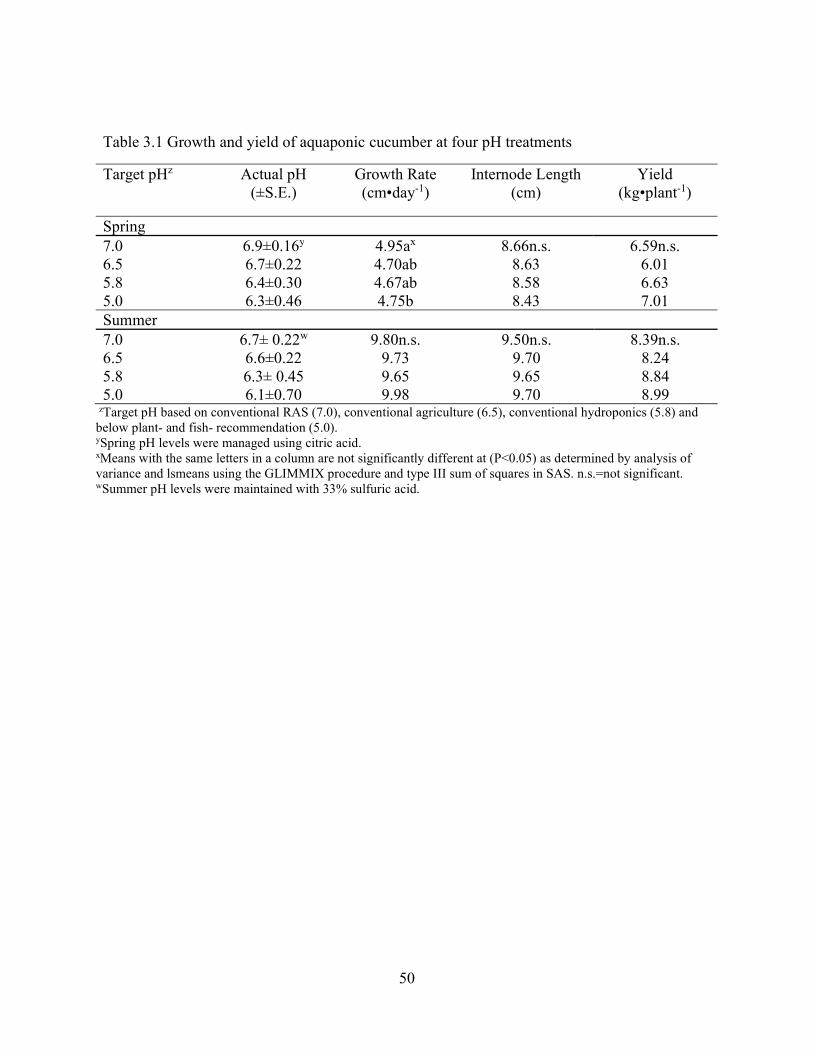
50

Table 3.1 Growth and yield of aquaponic cucumber at four pH treatments

Target pHz Actual pH (±S.E.)

Growth Rate (cm•day-1)

Internode Length (cm)

Yield (kg•plant-1)

Spring 7.0 6.9±0.16y 4.95ax 8.66n.s. 6.59n.s. 6.5 6.7±0.22 4.70ab 8.63 6.01 5.8 6.4±0.30 4.67ab 8.58 6.63 5.0 6.3±0.46 4.75b 8.43 7.01 Summer 7.0 6.7± 0.22w 9.80n.s. 9.50n.s. 8.39n.s. 6.5 6.6±0.22 9.73 9.70 8.24 5.8 6.3± 0.45 9.65 9.65 8.84 5.0 6.1±0.70 9.98 9.70 8.99

zTarget pH based on conventional RAS (7.0), conventional agriculture (6.5), conventional hydroponics (5.8) and below plant- and fish- recommendation (5.0). ySpring pH levels were managed using citric acid. xMeans with the same letters in a column are not significantly different at (P<0.05) as determined by analysis of variance and lsmeans using the GLIMMIX procedure and type III sum of squares in SAS. n.s.=not significant. wSummer pH levels were maintained with 33% sulfuric acid.

51

Table 3.2 Mid-Season macronutrient analysis of aquaponic irrigation water at four pH treatmentszy

Target pH Actual pH (±S.E.)

NO3-N P K Ca Mg

Springx 7.0 6.9±0.16 187n.s.w 8n.s. 104n.s. 187n.s. 20n.s. 6.5 6.7±0.22 183 8 104 186 20 5.8 6.4±0.30 184 8 104 188 20 5.0 6.3±0.46 171 8 104 187 20 Significance N/A N/A N/A N/A N/A N/A Summerv

7.0 6.7± 0.22 93a 11.n.s. 175a 108n.s. 20n.s. 6.5 6.6±0.22 86bc 11 173b 106 19 5.8 6.3± 0.45 88b 12 173b 106 19 5.0 6.1±0.70 85c 12 172b 105 19 Significance N/A N/A N/A L*u N/A N/A Recommended Levelt

N/A 216u 58 286 185 185 zAll units are in mg·L–1 yWhen compared against standard hydroponic solution for cucumber production (Resh, 2008), all measured levels of plant-essential elements were lower than the recommended amount for hydroponic production according to t-test results using the TTEST procedure in SAS. xSpring pH levels were managed using citric acid. wMeans with the same letters in a column are not significantly different at (P<0.05) as determined by analysis of variance and lsmeans using the GLIMMIX procedure and type III sum of squares in SAS. n.s.=not significant. vSummer pH levels were maintained with 33% sulfuric acid. uSignificance established using trend analyses in PROC GLIMMIX. L= linear trend. *= significance at alpha=0.05. N/A= no trend test conducted because of non-significant ANOVA. tSufficiency levels obtained from Jones, 2005. uppm total nitrogen

52

Table 3.3 Mid-season foliar analysis of macronutrients as percentage of dry matter for aquaponic cucumbers at four pH treatmentsz

Target pH Actual pH (±S.E.)

N P K Ca Mg S

Springy

7.0 6.9±0.16 4.98n.s.x 0.68a 3.95n.s. 8.36n.s. 0.58n.s. 0.76n.s. 6.5 6.7±0.22 4.96 0.52b 3.65 8.16 0.56 0.74 5.8 6.4±0.30 4.88 0.54b 3.59 7.65 0.54 0.74 5.0 6.3±0.46 4.90 0.57b 3.31 8.28 0.58 0.74 Significancew N/A N/A Q* N/A N/A N/A N/A Summerv

7.0 6.7± 0.22 5.72ab 0.62a 3.19n.s. 4.56n.s. 0.46n.s. 0.98n.s. 6.5 6.6±0.22 5.57c 0.51b 3.38 4.71 0.51 0.90 5.8 6.3± 0.45 5.85a 0.54b 3.18 4.10 0.51 1.09 5.0 6.1±0.70 5.68bc 0.51b 3.31 4.47 0.46 1.03 Significance N/A N/A L* N/A N/A N/A N/A Sufficiency Levelsu

N/A 4.30 0.30 3.10 2.40 0.35 0.32

zWhen compared against standard percentages in cucumber dry matter (Mills and Jones, 1996), all nutrients were above the lower range of recommended percentage of dry matter for cucumber growth according to t-test results using the TTEST procedure in SAS. ySpring pH levels were managed using citric acid. xMeans with the same letters in a column are not significantly different at (P<0.05) as determined by analysis of variance and lsmeans using the GLIMMIX procedure and type III sum of squares in SAS. n.s.=not significant. wSignifiance established using trend analyses in PROC GLIMMIX. L=linear trend, Q=quadratic trend. *= significance at alpha=0.05. N/A= no trend test conducted because of non-significant ANOVA. vSummer pH levels were maintained with 33% sulfuric acid. uSufficiency levels obtained from Mills and Jones, 1996.

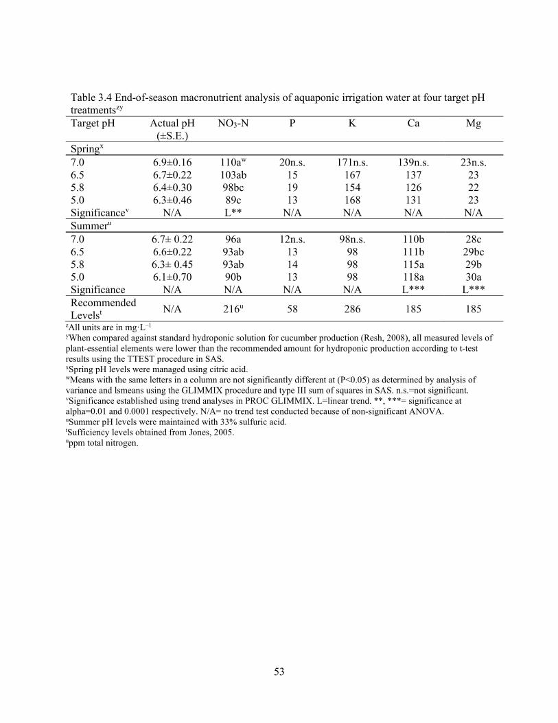
53

Table 3.4 End-of-season macronutrient analysis of aquaponic irrigation water at four target pH treatmentszy

Target pH Actual pH (±S.E.)

NO3-N P K Ca Mg

Springx

7.0 6.9±0.16 110aw 20n.s. 171n.s. 139n.s. 23n.s. 6.5 6.7±0.22 103ab 15 167 137 23 5.8 6.4±0.30 98bc 19 154 126 22 5.0 6.3±0.46 89c 13 168 131 23 Significancev N/A L** N/A N/A N/A N/A Summeru

7.0 6.7± 0.22 96a 12n.s. 98n.s. 110b 28c 6.5 6.6±0.22 93ab 13 98 111b 29bc 5.8 6.3± 0.45 93ab 14 98 115a 29b 5.0 6.1±0.70 90b 13 98 118a 30a Significance N/A N/A N/A N/A L*** L*** Recommended Levelst

N/A 216u 58 286 185 185 zAll units are in mg·L–1 yWhen compared against standard hydroponic solution for cucumber production (Resh, 2008), all measured levels of plant-essential elements were lower than the recommended amount for hydroponic production according to t-test results using the TTEST procedure in SAS. xSpring pH levels were managed using citric acid. wMeans with the same letters in a column are not significantly different at (P<0.05) as determined by analysis of variance and lsmeans using the GLIMMIX procedure and type III sum of squares in SAS. n.s.=not significant. vSignificance established using trend analyses in PROC GLIMMIX. L=linear trend. **, ***= significance at alpha=0.01 and 0.0001 respectively. N/A= no trend test conducted because of non-significant ANOVA. uSummer pH levels were maintained with 33% sulfuric acid. tSufficiency levels obtained from Jones, 2005. uppm total nitrogen.

54

Table 3.5 End-of-season foliar analysis of macronutrients as percentage of dry matter for aquaponic cucumbers at four target pH treatmentsz

Target pH Actual pH (±S.E.)

N P K Ca Mg S

Springy

7.0 6.9±0.16 5.26n.s.x 0.54n.s. 4.11n.s. 5.46n.s. 0.41n.s. 1.23n.s. 6.5 6.7±0.22 5.16 0.44 4.06 5.61 0.42 1.19 5.8 6.4±0.30 4.84 0.44 3.82 4.92 0.40 1.07 5.0 6.3±0.46 5.23 0.55 4.08 5.52 0.43 1.20 Significancew N/A N/A N/A N/A N/A N/A N/A Summerv

7.0 6.7± 0.22 3.94n.s. 0.38a 2.70n.s. 8.85ab 0.59n.s. 1.45n.s. 6.5 6.6±0.22 4.48 0.32b 2.50 8.99a 0.63 1.43 5.8 6.3± 0.45 5.10 0.33b 2.52 8.54bc 0.62 1.51 5.0 6.1±0.70 5.16 0.34b 2.66 8.24c 0.62 1.54 Significance N/A N/A N/A N/A L* N/A N/A Sufficiency Levelsu

N/A 4.30 0.30 3.10 2.40 0.35 0.32

zWhen compared against standard percentages in cucumber dry matter (Mills and Jones, 1996), all nutrients were above the lower range of recommended percentage of dry matter for cucumber growth according to t-test results using the TTEST procedure in SAS. ySpring pH levels were managed using citric acid. xMeans with the same letters in a column are not significantly different at (P<0.05) as determined by analysis of variance and lsmeans using the GLIMMIX procedure and type III sum of squares in SAS. n.s.=not significant. wSignificance established using trend analyses in PROC GLIMMIX. L=linear trend. *= significance at alpha=0.05. N/A= no trend test conducted because of non-significant ANOVA. vSummer pH levels were maintained with 33% sulfuric acid. uSufficiency levels obtained from Mills and Jones, 1996.

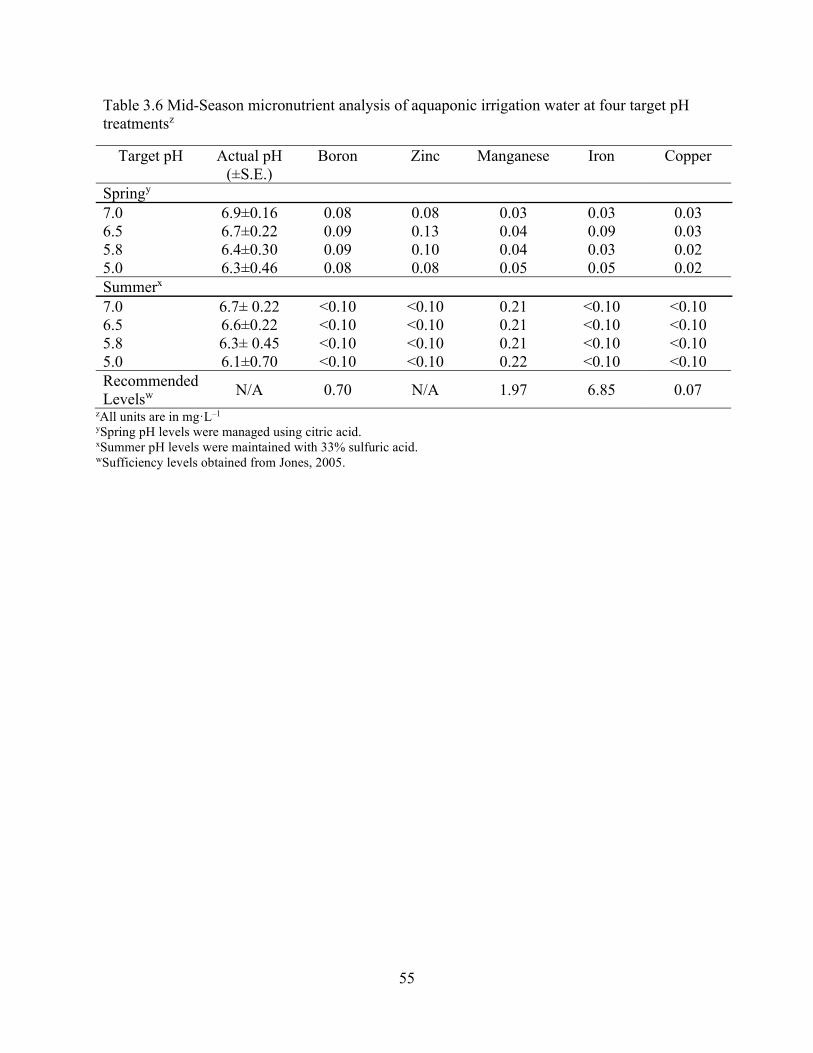
55

Table 3.6 Mid-Season micronutrient analysis of aquaponic irrigation water at four target pH treatmentsz

Target pH Actual pH (±S.E.)

Boron Zinc Manganese Iron Copper

Springy 7.0 6.9±0.16 0.08 0.08 0.03 0.03 0.03 6.5 6.7±0.22 0.09 0.13 0.04 0.09 0.03 5.8 6.4±0.30 0.09 0.10 0.04 0.03 0.02 5.0 6.3±0.46 0.08 0.08 0.05 0.05 0.02 Summerx

7.0 6.7± 0.22 <0.10 <0.10 0.21 <0.10 <0.10 6.5 6.6±0.22 <0.10 <0.10 0.21 <0.10 <0.10 5.8 6.3± 0.45 <0.10 <0.10 0.21 <0.10 <0.10 5.0 6.1±0.70 <0.10 <0.10 0.22 <0.10 <0.10 Recommended Levelsw

N/A 0.70 N/A 1.97 6.85 0.07 zAll units are in mg·L–1 ySpring pH levels were managed using citric acid. xSummer pH levels were maintained with 33% sulfuric acid. wSufficiency levels obtained from Jones, 2005.

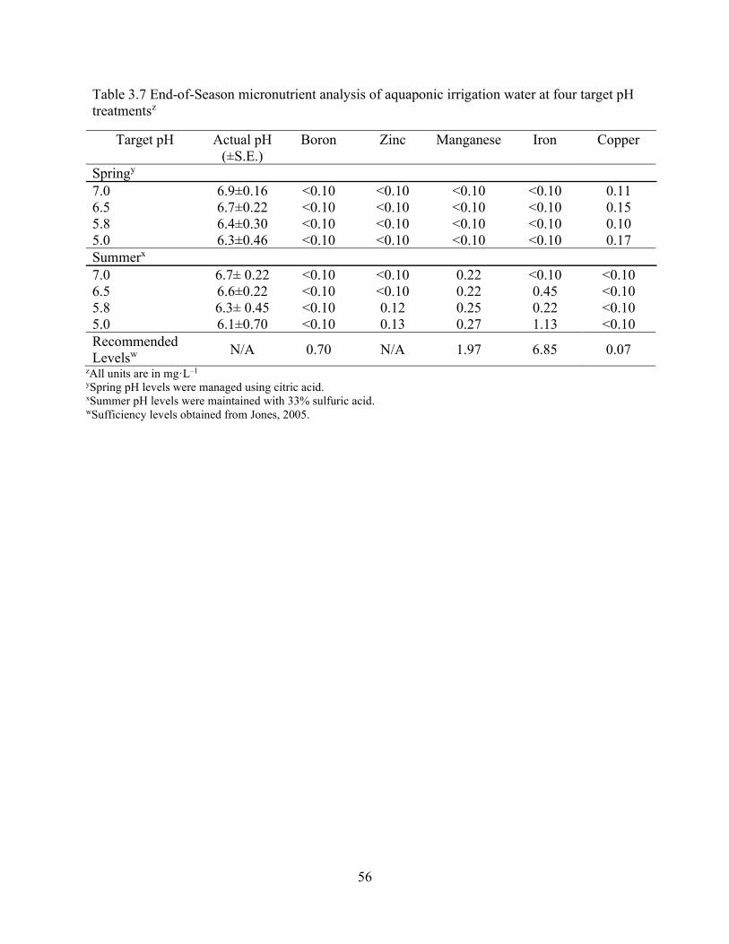
56

Table 3.7 End-of-Season micronutrient analysis of aquaponic irrigation water at four target pH treatmentsz

Target pH Actual pH (±S.E.)

Boron Zinc Manganese Iron Copper

Springy 7.0 6.9±0.16 <0.10 <0.10 <0.10 <0.10 0.11 6.5 6.7±0.22 <0.10 <0.10 <0.10 <0.10 0.15 5.8 6.4±0.30 <0.10 <0.10 <0.10 <0.10 0.10 5.0 6.3±0.46 <0.10 <0.10 <0.10 <0.10 0.17 Summerx

7.0 6.7± 0.22 <0.10 <0.10 0.22 <0.10 <0.10 6.5 6.6±0.22 <0.10 <0.10 0.22 0.45 <0.10 5.8 6.3± 0.45 <0.10 0.12 0.25 0.22 <0.10 5.0 6.1±0.70 <0.10 0.13 0.27 1.13 <0.10 Recommended Levelsw

N/A 0.70 N/A 1.97 6.85 0.07 zAll units are in mg·L–1 ySpring pH levels were managed using citric acid. xSummer pH levels were maintained with 33% sulfuric acid. wSufficiency levels obtained from Jones, 2005.

57

zWhen compared against standard percentages in cucumber dry matter (Mills and Jones, 1996), all nutrients were above the lower range of recommended percentage of dry matter for cucumber growth according to t-test results using the TTEST procedure in SAS. ySpring pH levels were managed using citric acid. xMeans with the same letters in a column are not significantly different at (P<0.05) as determined by analysis of variance and lsmeans using the GLIMMIX procedure and type III sum of squares in SAS. n.s.=not significant. wSummer pH levels were maintained with 33% sulfuric acid. vSignificance established using trend analyses in PROC GLIMMIX. Q=quadratic trend. *= significance at alpha=0.05. N/A= no trend test conducted because of non-significant ANOVA. uSufficiency levels obtained from Mills and Jones, 1996.

Table 3.8 Mid-season foliar analysis of micronutrients as dry matter for aquaponic cucumbers at four pH treatmentsz

Target pH Actual pH (±S.E.)

B Zn Mn Fe Cu

Springy

7.0 6.9±0.16 60n.s.x 95n.s. 46n.s. 106n.s. 12n.s. 6.5 6.7±0.22 57 84 47 116 12 5.8 6.4±0.30 55 82 46 120 11 5.0 6.3±0.46 59 92 47 119 12 Significance N/A N/A N/A N/A N/A N/A Summerw

7.0 6.7± 0.22 43n.s. 80n.s. 184ab 144n.s. 11n.s. 6.5 6.6±0.22 38 61 118c 78 9 5.8 6.3± 0.45 40 62 166b 89 10 5.0 6.1±0.70 38 79 214a 86 10 Significance N/A N/A N/A Q*v N/A N/A Sufficiency Levelsu

N/A 30 25 50 50 8

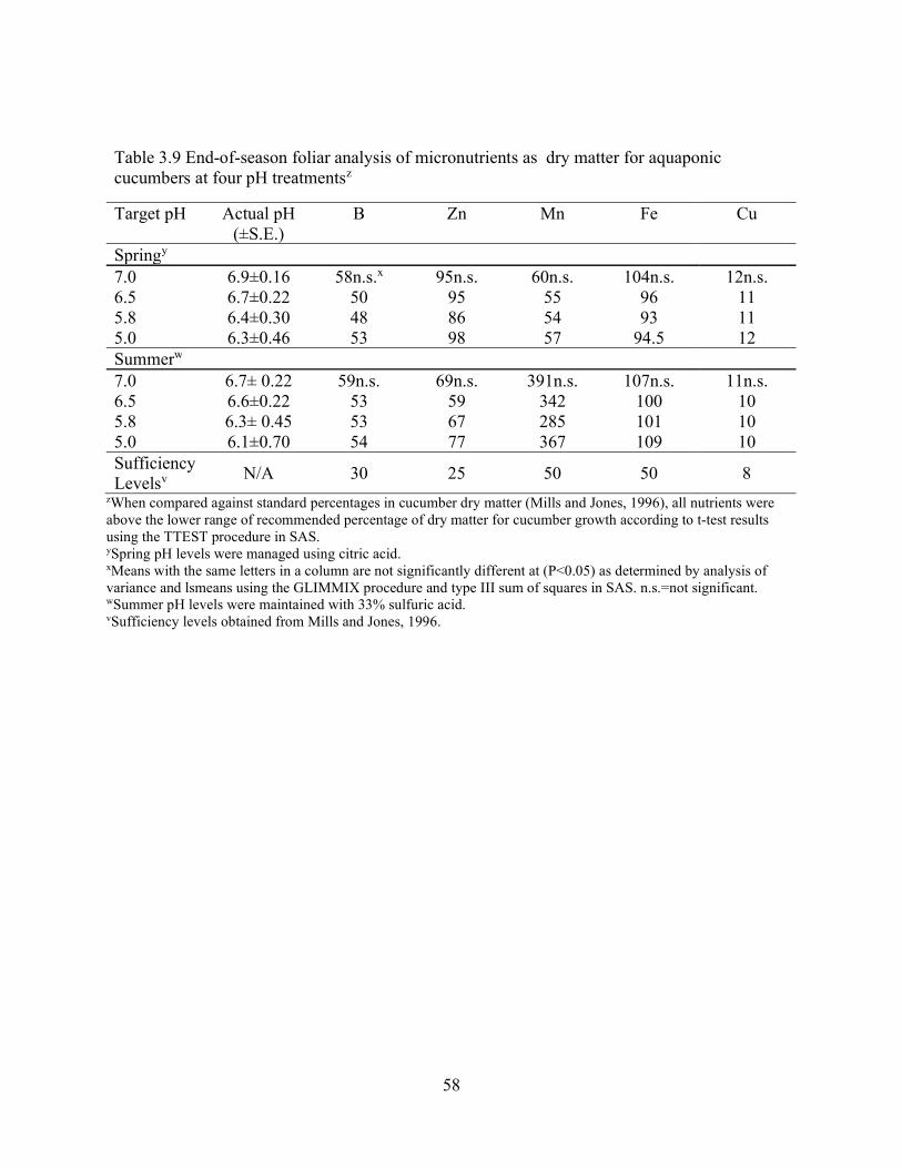
58

Table 3.9 End-of-season foliar analysis of micronutrients as dry matter for aquaponic cucumbers at four pH treatmentsz

Target pH Actual pH (±S.E.)

B Zn Mn Fe Cu

Springy

7.0 6.9±0.16 58n.s.x 95n.s. 60n.s. 104n.s. 12n.s. 6.5 6.7±0.22 50 95 55 96 11 5.8 6.4±0.30 48 86 54 93 11 5.0 6.3±0.46 53 98 57 94.5 12 Summerw

7.0 6.7± 0.22 59n.s. 69n.s. 391n.s. 107n.s. 11n.s. 6.5 6.6±0.22 53 59 342 100 10 5.8 6.3± 0.45 53 67 285 101 10 5.0 6.1±0.70 54 77 367 109 10 Sufficiency Levelsv

N/A 30 25 50 50 8 zWhen compared against standard percentages in cucumber dry matter (Mills and Jones, 1996), all nutrients were above the lower range of recommended percentage of dry matter for cucumber growth according to t-test results using the TTEST procedure in SAS. ySpring pH levels were managed using citric acid. xMeans with the same letters in a column are not significantly different at (P<0.05) as determined by analysis of variance and lsmeans using the GLIMMIX procedure and type III sum of squares in SAS. n.s.=not significant. wSummer pH levels were maintained with 33% sulfuric acid. vSufficiency levels obtained from Mills and Jones, 1996.

59

Table 3.10 Macronutrients (mg • kg dried solids-1) contained in suspended solids of aquaculture effluentz

P K S Ca Mg pH Pre-

Plant Post-Plant

Pre-Plant

Post-Plant

Pre-Plant

Post-Plant

Pre-Plant

Post-Plant

Pre-Plant

Post-Plant

7.0 2075 1672 757 519 1050 850 1713 2825 300 300 6.5 2628 2392 591 498 1100 875 2625 4188 325 300 5.8 1892 1580 716 540 1150 925 5100 5013 350 400 5.0 1693 2037 747 581 1213 963 3550 3238 350 325

zSolids were dried at 105°C for 24h before analysis.

60

Table 3.11 Micronutrients (mg • kg dried solids-1) contained in suspended solids of aquaculture effluentz B Zn Mn Fe Cu pH Pre-

Plant Post-Plant

Pre-Plant

Post-Plant

Pre-Plant

Post-Plant

Pre-Plant

Post-Plant

Pre-Plant

Post-Plant

7.0 5 13 175 150 625 1250 850 938 25 25

6.5 5 1 188 38 338 600 963 488 25 13

5.8 5 1 125 150 450 2238 1038 813 25 13

5.0 1 1 13 150 13 1963 1113 1125 25 13 zSolids were dried at 105°C for 24h before analysis.

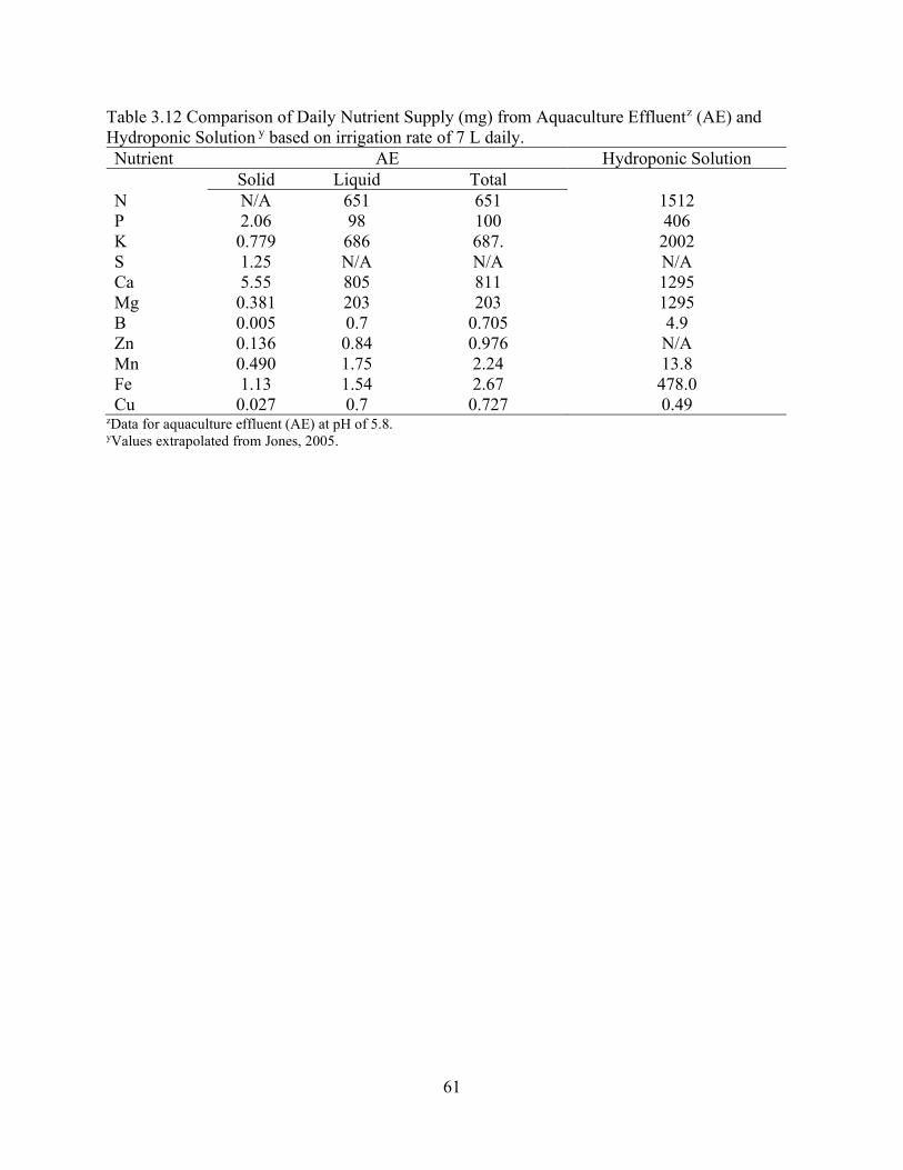
61

Table 3.12 Comparison of Daily Nutrient Supply (mg) from Aquaculture Effluentz (AE) and Hydroponic Solution y based on irrigation rate of 7 L daily.

Nutrient AE Hydroponic Solution

Solid Liquid Total

N N/A 651 651 1512 P 2.06 98 100 406 K 0.779 686 687. 2002 S 1.25 N/A N/A N/A Ca 5.55 805 811 1295 Mg 0.381 203 203 1295 B 0.005 0.7 0.705 4.9 Zn 0.136 0.84 0.976 N/A Mn 0.490 1.75 2.24 13.8 Fe 1.13 1.54 2.67 478.0 Cu 0.027 0.7 0.727 0.49

zData for aquaculture effluent (AE) at pH of 5.8. yValues extrapolated from Jones, 2005.

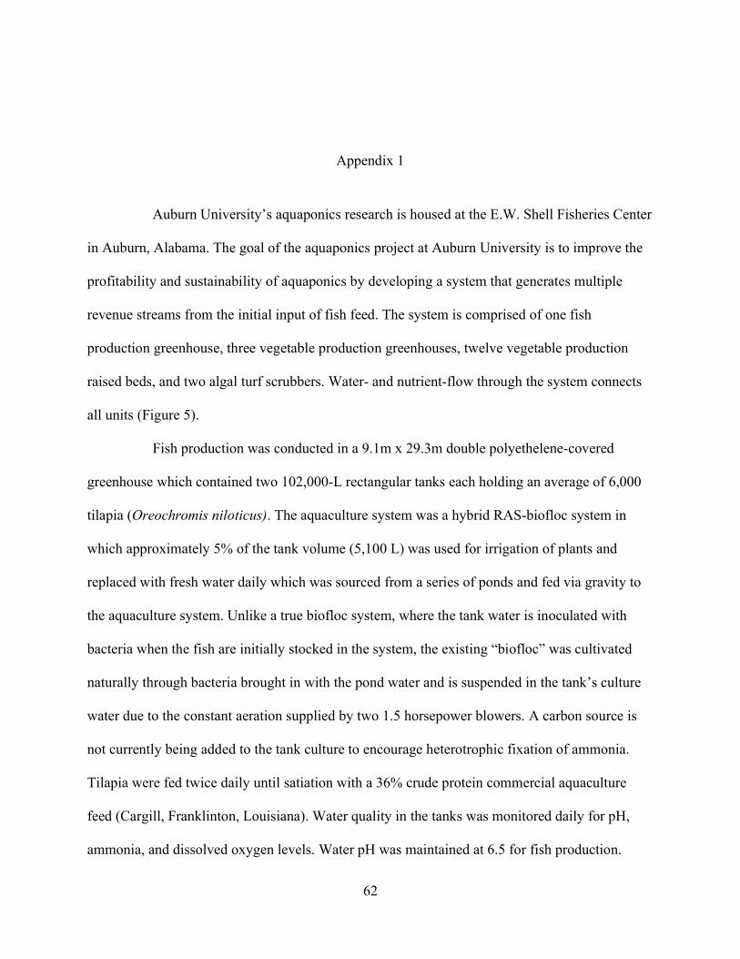
62

Appendix 1

Auburn University’s aquaponics research is housed at the E.W. Shell Fisheries Center

in Auburn, Alabama. The goal of the aquaponics project at Auburn University is to improve the

profitability and sustainability of aquaponics by developing a system that generates multiple

revenue streams from the initial input of fish feed. The system is comprised of one fish

production greenhouse, three vegetable production greenhouses, twelve vegetable production

raised beds, and two algal turf scrubbers. Water- and nutrient-flow through the system connects

all units (Figure 5).

Fish production was conducted in a 9.1m x 29.3m double polyethelene-covered

greenhouse which contained two 102,000-L rectangular tanks each holding an average of 6,000

tilapia (Oreochromis niloticus). The aquaculture system was a hybrid RAS-biofloc system in

which approximately 5% of the tank volume (5,100 L) was used for irrigation of plants and

replaced with fresh water daily which was sourced from a series of ponds and fed via gravity to

the aquaculture system. Unlike a true biofloc system, where the tank water is inoculated with

bacteria when the fish are initially stocked in the system, the existing “biofloc” was cultivated

naturally through bacteria brought in with the pond water and is suspended in the tank’s culture

water due to the constant aeration supplied by two 1.5 horsepower blowers. A carbon source is

not currently being added to the tank culture to encourage heterotrophic fixation of ammonia.

Tilapia were fed twice daily until satiation with a 36% crude protein commercial aquaculture

feed (Cargill, Franklinton, Louisiana). Water quality in the tanks was monitored daily for pH,

ammonia, and dissolved oxygen levels. Water pH was maintained at 6.5 for fish production.

63

Ammonia and dissolved oxygen levels remained within acceptable levels for fish production for

the duration of the experiment. Suspended solids, including uneaten feed, feces, and biofloc were

settled and removed from aquaculture effluent (AE) using two passive clarifiers connected in a

series. The clarifiers were 1,500-L cone-bottom tanks located adjacent to the aquaculture system

outside the greenhouse. Aquaculture effluent was continuously pumped into the first clarifier

using an air lift and was forced to pass under a solid baffle separating the tank into two halves

before being moved to the second clarifier which was used as the irrigation reservoir for the plant

greenhouse. The clarifiers removed an average of 50% of suspended solids from AE before it

was used to irrigate plants.

Water is captured from greenhouse production in one of four 378-L sumps and is

used in algae production and research. Unlike conventional aquaponic systems, the Auburn

system contains a high amount of suspended solids, which places it in a unique position for

research.

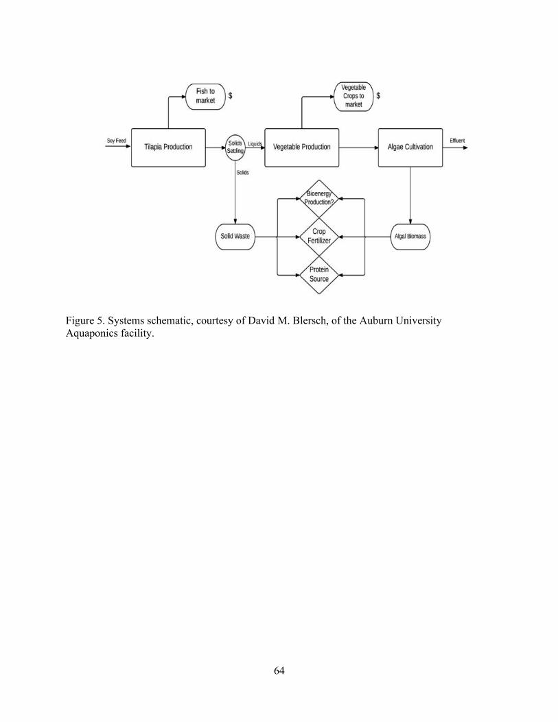
64

Figure 5. Systems schematic, courtesy of David M. Blersch, of the Auburn University Aquaponics facility.