biophysical chemistry of biointerfaces (ohshima/biophysical chemistry of biointerfaces) || potential...

2 Potential Distribution Around aNonuniformly Charged Surfaceand Discrete Charge Effects

2.1 INTRODUCTION

In the previous chapter we assumed that particles have uniformly charged hard sur-

faces. This is called the smeared charge model. Electric phenomena on the particle

surface are usually discussed on the basis of this model [1–4]. In this chapter we

present a general method of solving the Poisson–Boltzmann equation for the elec-

tric potential around a nonuniformly charged hard surface. This method enables us

to calculate the potential distribution around surfaces with arbitrary fixed surface

charge distributions. With this method, we can discuss the discrete nature of

charges on a particle surface (the discrete charge effects).

2.2 THE POISSON–BOLTZMANN EQUATION FOR A SURFACEWITHAN ARBITRARY FIXED SURFACE CHARGE DISTRIBUTION

Here we treat a planar plate surface immersed in an electrolyte solution of relative

permittivity er and Debye–Huckel parameter k. We take x- and y-axes parallel to theplate surface and the z-axis perpendicular to the plate surface with its origin at the

plate surface so that the region z> 0 corresponds to the solution phase (Fig. 2.1).

First we assume that the surface charge density s varies in the x-direction so that sis a function of x, that is, s¼ s(x). The electric potential c is thus a function of xand z. We assume that the potential c(x, z) satisfies the following two-dimensional

linearized Poison–Boltzmann equation, namely,

@2

@x2þ @2

@z2

� �cðx; zÞ ¼ k2cðx; zÞ ð2:1Þ

Equation (2.1) is subject to the following boundary conditions at the plate surface

and far from the surface:

@cðx; zÞ@z

��z¼0

¼ � sðxÞereo

ð2:2Þ

Biophysical Chemistry of Biointerfaces By Hiroyuki OhshimaCopyright# 2010 by John Wiley & Sons, Inc.

47

and

cðx; zÞ ! 0;@c@z

! 0 as z ! 1 ð2:3Þ

To solve Eq. (2.1) subject to Eq. (2.3), we write c(x, z) and s(x) by their Fourier

transforms,

cðx; zÞ ¼ 1

2p

Zcðk; zÞeikx dk ð2:4Þ

sðxÞ ¼ 1

2p

ZsðkÞeiks dk ð2:5Þ

where cðx; zÞ and sðkÞ are the Fourier coefficients. We thus obtain

cðk; zÞ ¼Zcðx; zÞe�iks dx ð2:6Þ

sðkÞ ¼ZsðxÞe�ikx dx ð2:7Þ

Substituting Eq. (2.4) into Eq. (2.1) subject to Eq. (2.3), we have

@2cðk; zÞ@z2

¼ ðk2 þ k2Þcðk; zÞ ð2:8Þ

which is solved to give

cðk; zÞ ¼ CðkÞexpð�ffiffiffiffiffiffiffiffiffiffiffiffiffiffiffik2 þ k2

pzÞ ð2:9Þ

x

y

z

O

FIGURE 2.1 A charged plate in an electrolyte solution. The x- and y-axes are taken to be

parallel to the plate surface and the z-axis perpendicular to the plate.

48 POTENTIAL DISTRIBUTION AROUND A NONUNIFORMLY CHARGED SURFACE

where C(k) is the Fourier coefficient independent of z. Equation (2.4) thus becomes

cðx; zÞ ¼ZCðkÞexp½ikx� z

ffiffiffiffiffiffiffiffiffiffiffiffiffiffiffik2 þ k2

p�dk ð2:10Þ

The unknown coefficient C(k) can be determined to satisfy the boundary condition

(Eq. (2.2)) to give

CðkÞ ¼ sðkÞereo


p ð2:11Þ

Substituting Eq. (2.11) into Eq. (2.10), we have

cðx; zÞ ¼ 1

2pereo

ZsðkÞffiffiffiffiffiffiffiffiffiffiffiffiffiffiffik2 þ k2

p exp ikx�ffiffiffiffiffiffiffiffiffiffiffiffiffiffiffik2 þ k2

pz

h idk ð2:12Þ

which is the general expression for c(x, z).Consider several cases of charge distributions.

(i) Uniform smeared charge density Consider a plate with a uniform surface

charge density s

sðxÞ ¼ s ð2:13Þ

From Eq. (2.7), we have

sðkÞ ¼ sZexpð�ikxÞdx ¼ 2psdðkÞ ð2:14Þ

where d(k) is Dirac’s delta function and we have used the following rela-

tion:

dðkÞ ¼ 1

2p

ZexpðikxÞdx ð2:15Þ

Substituting this result into Eq. (2.12), we have

cðx; zÞ ¼ sereo

ZdðkÞffiffiffiffiffiffiffiffiffiffiffiffiffiffiffik2 þ k2

p exp ikx�ffiffiffiffiffiffiffiffiffiffiffiffiffiffiffik2 þ k2

pz

h idk ð2:16Þ

Carrying out the integration, we obtain

cðzÞ ¼ sereok

e�kz ð2:17Þ

THE POISSON–BOLTZMANN EQUATION FOR A SURFACE 49

which is independent of x and agrees with Eq. (1.25) combined with

Eq. (1.26), as expected.

(ii) Sinusoidal charge distribution Consider the case where the surface charge

density s(x) varies sinusoidally (Fig. 2.2), namely,

sðxÞ ¼ cosðqxÞ ð2:18ÞFrom Eq. (2.7), we have

sðkÞ ¼ZcosðqxÞe�ikx dx

¼ 1

2

Zðeiqx þ e�iqxÞe�ikx dx

¼ s2ð2pÞ dðk þ qÞ þ dðk � qÞf g

ð2:19Þ


cðx; zÞ ¼ s2ereo

Zdðk þ qÞ þ dðk � qÞf gffiffiffiffiffiffiffiffiffiffiffiffiffiffiffi

k2 þ k2p exp ikx�


pz

h idk

¼ s2ereo

1ffiffiffiffiffiffiffiffiffiffiffiffiffiffiffik2 þ q2

p exp iqx�ffiffiffiffiffiffiffiffiffiffiffiffiffiffiffiq2 þ k2

pz

h iþ exp �iqx�

ffiffiffiffiffiffiffiffiffiffiffiffiffiffiffiq2 þ k2

pz

h i

¼ sereo

cosðqxÞffiffiffiffiffiffiffiffiffiffiffiffiffiffiffik2 þ q2

p exp �ffiffiffiffiffiffiffiffiffiffiffiffiffiffiffiq2 þ k2

pz

h ið2:20Þ

When q¼ 0, Eq. (2.20) reduces to Eq. (2.17) for the uniform charge distri-

bution case. Figure 2.3 shows an example of the potential distribution

c(x, z) calculated from Eq. (2.20). It is to be noted that comparison of Eqs.

(2.20) and (2.18) shows

cðx; zÞ ¼ sðxÞereo

exp½�ffiffiffiffiffiffiffiffiffiffiffiffiffiffiffiq2 þ k2

pz�ffiffiffiffiffiffiffiffiffiffiffiffiffiffiffi

k2 þ q2p ð2:21Þ

FIGURE 2.2 A plate surface with a sinusoidal charge distribution.


That is, in this case the surface potential c(x, z) is proportional to the sur-

face charge density s(x).The surface potential c(x, 0) calculated from Eq. (2.20) is given by

cðx; 0Þ ¼ sereo

cosðqxÞffiffiffiffiffiffiffiffiffiffiffiffiffiffiffik2 þ q2

p ð2:22Þ

which is a function of x.

(iii) Sigmoidal distribution We treat a planar charged plate with a gradient in

surface charge density, which is s1 at one end and s2 at the other, varying

sigmoidally between s1 and s2 along the plate surface [5] (Fig. 2.4). We

may thus assume that the surface charge density s varies in the x-directionaccording to the following form:

sðxÞ ¼ s1 þ s2 � s11þ expð�bxÞ

¼ 1

2ðs1 þ s2Þ þ 1

2ðs2 � s1Þtanh bx

2

� � ð2:23Þ

where b(�0) is a parameter proportional to the slope of s(x) at x¼ 0.

An example of charge distribution calculated for several values of b/k at

FIGURE 2.3 Scaled potential distribution c�(x, z) =c(x, z)/(s/ereok) around a surface witha sinusoidal charge density distribution s(x) = s cos(qx) as a function of kx and kz, where kxand kz are the scaled distances in the x and y directions, respectively. Calculated for q/k = 1.


s2/s1¼ 3 is given in Fig. 2.5. From Eq. (2.7), we have

sðkÞ ¼ 1

2ðs1 þ s2ÞdðkÞ � iðs2 � s1Þ

b sinhðpk=bÞ� �

ð2:24Þ

Then by substituting Eq. (2.23) into Eq. (2.12), we obtain the solution to

Eq. (2.1) as

cðx; zÞ ¼ ðs1 þ s2Þ2ereok

e�kz þ ðs2 � s1Þbereo

Z 1

0

expð�kzffiffiffiffiffiffiffiffiffiffiffiffit2 þ 1

p ÞsinðkxtÞffiffiffiffiffiffiffiffiffiffiffiffit2 þ 1

psinhðpkt=bÞ dt ð2:25Þ

FIGURE 2.4 A plate surface with a sigmoidal gradient in surface charge density. The

surface charge density s varies in the x-direction. s(x) tends to s1 as x!�1 and to s2 asx!+1, varying sigmoidally around x= 0. From Ref. 5.

FIGURE 2.5 Sigmoidal distribution of reduced surface charge density s�(x), defined by

s�(x) = 2s(x)/(s1 +s2), as a function of kx for several values of b/k at s2/s1 = 3. The limiting

case b/k=1 corresponds to a sharp boundary between two regions of s1 and s2. The oppo-site limiting case b/k = 0 corresponds to a uniform charge distribution with a density

(s1 + s2)/2. From Ref. 5.


which gives the potential distribution c (x, z) around a charged plate

with a sigmoidal gradient in surface charge density given by Eq. (2.23)

as a function of x and z. The first term on the right-hand side of Eq.

(2.25) corresponds to the potential for a plate carrying the average

charge of s1 and s2. Equation (2.25) corresponds to the situation in

which there is no flow of electrolyte ions along the plate surface, al-

though a potential gradient (i.e., electric field) is formed along the plate

surface. The potential gradient is counterbalanced by the concentration

gradient of electrolyte ions. The electrochemical potential of electrolyte

ions thus takes the same value everywhere in the solution phase so that

there is no ionic flow.

To calculate the potential distribution via Eq. (2.25), one needs numeri-

cal integration. Figure 2.6 shows an example of the numerical calculation of

c(x, z) for b/k¼ 1 at s2/s1¼ 3. As will be shown later, the potential c(x, z)is not always proportional to the surface charge density s(x) unlike the casewhere the plate is uniformly charged (s¼ constant).

We now consider several limiting cases of Eq. (2.25).

(a) When b=k � 1, Eq. (2.25) tends to the following limiting value:

cðx; zÞ ¼ s1 þ s22ereok

expð�kzÞ þ 2ðs2 � s1Þpðs1 þ s2Þ

Z 1

0


p ÞsinðkxtÞt

ffiffiffiffiffiffiffiffiffiffiffiffit2 þ 1

p dt

" #

ð2:26Þ

*(x,z)

z

x

–10 –8 –6 –4 –2 0 2 4 6 8 10

0

2

1

1.2

1.4

0.8

0.6

1.6

1

0.2

0.6

0.4

1.8

0.81.2

1.41.6

0.40.2

FIGURE 2.6 Reduced potential distribution c(x, z) = 2ereokc(x, z)/(s1 + s2) around a sur-

face with a sigmoidal gradient in surface charge density as a function of kx and kz calculatedfrom Eq. (2.25) for b/k¼ 1 at s2/s1¼ 3. From Ref. 5.


which is independent of b/k. Note that even in the limit of b/k¼1,

which corresponds to a sharp boundary between two regions of s1 ands2 (Eq. (2.23)), the potential varies sigmoidally in the x-direction unlike

s(x). This will be seen later again in Fig. 2.7, which shows the surface

potential c(x, 0).(b) In the opposite limit b=k � 1 (the charge gradient becomes small),

Eq. (2.25) becomes


expð�kzÞ ð2:27Þ

Equation (2.27), which is independent of b/k and x, coincides with the

potential distribution produced by a plate with a uniform charge density

(s1 + s2)/2 (the mean value of s1 and s2), as expected.(c) When kz � 1, Eq. (2.25) becomes


expð�kzÞ þ s2 � s1s1 þ s2

� �tanh

bx2

� �expð�kzÞ

� �

¼ sðxÞereok

ð2:28Þ

That is, the potential c(x, z) becomes directly proportional to the surface

charge density s(x) in the region far from the plate surface, as in the

case of uniform charge distribution (s¼ constant). The x-dependence ofc(x, z) thus becomes identical to that of s(x). It must be emphasized

here that this is the case only for kz � 1 and in general c(x, z) is notproportional to s(x).

(d) As kx!�1 or kx! +1, Eq. (2.25) tends to

cðx; zÞ ¼ s1ereok

expð�kzÞ as x ! �1 ð2:29Þ

cðx; zÞ ¼ s2ereok

expð�kzÞ as x ! þ1 ð2:30Þ

The potential distribution given by Eq. (2.29) (or Eq. (2.30)) agrees with

that produced by a plate with surface charge density s1 (or s2), asexpected.

The surface potential of the plate, c(x, 0), is given by

cðx; 0Þ ¼ s1 þ s22ereok

1þ 2kðs2 � s1Þbðs1 þ s2Þ

Z 1

0

sinðkxtÞffiffiffiffiffiffiffiffiffiffiffiffit2 þ 1

psinhðpkt=bÞ dt

" #ð2:31Þ


Figure 2.7 shows the distribution of the surface potential c(x, 0) alongthe plate surface as a function of kx for several values of b/k at

s2/s1¼ 3. Each curve for c(x, 0) in Fig. 2.7 corresponds to a curve for

s(x) with the same value of b/k in Fig. 2.5. It is interesting to note that

even for the limiting case of b/k¼1, which corresponds to a sharp

boundary between two regions of s1 and s2, the potential does not

show a step function type distribution but varies sigmoidally unlike

s(x) in this limit.

We now derive expressions for the components of the electric field E (Ex, 0, Ez),

which are obtained by differentiating c(x, z) with respect to x or z, as potential gra-dient (i.e., electric field) is formed along the plate surface.

Ex ¼ � @c@x

¼ � s2 � s1ereob

kZ 1

0

t expð�kzffiffiffiffiffiffiffiffiffiffiffiffit2 þ 1

p ÞcosðkxtÞffiffiffiffiffiffiffiffiffiffiffiffit2 þ 1

psinhðpkt=bÞ dt ð2:32Þ

and

Ez ¼ � @c@z

¼ s1 þ s22ereo

expð�kzÞ þ 2kðs2 � s1Þbðs1 þ s2Þ

Z 1

0


p ÞsinðkxtÞsinhðpkt=bÞ dt

" #

ð2:33Þ

FIGURE 2.7 Distribution of the reduced surface potential c*(x, 0), defined by c�(x, 0) =2ereokc(x, 0)/(s1 +s2), along a surface with a sigmoidal gradient in surface charge density as

a function of kx for several values of b/k at s2/s1 = 3. From Ref. 5.


2.3 DISCRETE CHARGE EFFECT

In some biological surfaces, especially the low charge density case, the discrete na-

ture of the surface charge may become important. Here we treat a planar plate surface

carrying discrete charges immersed in an electrolyte solution of relative permittivity

er and Debye–Huckel parameter k. We take x- and y-axes parallel to the plate surfaceand the z-axis perpendicular to the plate surface with its origin at the plate surface so

that the region z> 0 corresponds to the solution phase (Fig. 2.8). We treat the case in

which the surface charge density s is a function of x and y, that is, s¼ s(x, y).The electric potential c is thus a function of x, y, and z. We assume that the potential

c(x, y, z) satisfies the following three-dimensional linearized Poison–Boltzmann

equation:

@2

@x2þ @2

@y2þ @2

@z2

� �cðx; y; zÞ ¼ k2cðx; y; zÞ ð2:34Þ

which is an extension of the two-dimensional linearized Poisson–Boltzmann equation

(2.1) to the three-dimensional case. Equation (2.34) is subject to the following bound-

ary conditions at the plate surface and far from the surface:

@cðx; y; zÞ@z

��z¼0

¼ � sðx; yÞereo

ð2:35Þ

and

cðx; y; zÞ ! 0;@cðx; y; zÞ

@z

��z¼0

! 0 as z ! 1 ð2:36Þ

In Eq. (2.35) we have assumed that the electric filed within the plate can be neglected.

x

y

z

+

+

+

+

+

+

+ +

+

++

+

++

++

O

FIGURE 2.8 Plate surface carrying discrete charges in an electrolyte solution.


To solve Eq. (2.34), we write c(x, y, z) and s(x, y) by their Fourier transforms,

cðrÞ ¼ 1

ð2pÞ2Z

cðk; zÞexpðik � sÞdk ð2:37Þ

sðsÞ ¼ 1

ð2pÞ2Z

sðkÞexpðik � sÞdk ð2:38Þ

with

r ¼ ðx; y; zÞ; s ¼ ðx; yÞ; and k ¼ ðkx; kyÞ ð2:39Þ

where cðk; zÞ and sðkÞ are the Fourier coefficients. We thus obtain

cðk; zÞ ¼Z

cðrÞexpð�ik � sÞds ð2:40Þ

sðkÞ ¼Z

sðsÞexpð�ik � sÞds ð2:41Þ


@2cðk; zÞ@z2

¼ ðk2 þ k2Þcðk; zÞ ð2:42Þ

where

k ¼ffiffiffiffiffiffiffiffiffiffiffiffiffiffiffik2x þ k2y

qð2:43Þ

Equation (2.42) is solved to give

cðk; zÞ ¼ AðkÞexpð�ffiffiffiffiffiffiffiffiffiffiffiffiffiffiffik2 þ k2

pzÞ ð2:44Þ

The unknown coefficient A(k) can be determined to satisfy the boundary condition

(Eq. (2.35)) to give

AðkÞ ¼ sðkÞereo


p ð2:45Þ

We thus obtain from Eq. (2.37)

cðrÞ ¼ 1

ð2pÞ2ereo

ZsðkÞffiffiffiffiffiffiffiffiffiffiffiffiffiffiffik2 þ k2

p expðik � sÞexpð�ffiffiffiffiffiffiffiffiffiffiffiffiffiffiffik2 þ k2

pzÞdk ð2:46Þ

This is the general expression for the electric potential c(x, y, z) around a plate

surface carrying a discrete charge s(x, y).

DISCRETE CHARGE EFFECT 57

Consider several cases of charge distributions.

(i) Uniform smeared charge density Consider a plate with a uniform surface

charge density s

sðsÞ ¼ s ð2:47Þ


sðkÞ ¼ sZ

expð�ik � sÞds

¼ ð2pÞ2sdðkÞð2:48Þ

where we have used the following relation:

dðkÞ ¼ 1

ð2pÞ2Z

expðik � sÞds ð2:49Þ


cðrÞ ¼ sereo

ZdðkÞffiffiffiffiffiffiffiffiffiffiffiffiffiffiffik2 þ k2

p expðik � sÞexpð�ffiffiffiffiffiffiffiffiffiffiffiffiffiffiffik2 þ k2

pzÞdk ð2:50Þ


cðrÞ ¼ sereok

e�kz ð2:51Þ

which agrees with Eq. (1.25) combined with Eq. (1.26), as expected.

(ii) A point charge Consider a plate carrying only one point charge q situated at(x, y)¼ (0, 0) (Fig. 2.9).

sðsÞ ¼ qdðsÞ ð2:52Þ


sðkÞ ¼ q

ZdðsÞexpð�ik � sÞds ¼ q ð2:53Þ


cðrÞ ¼ q

ð2pÞ2ereo

Z1ffiffiffiffiffiffiffiffiffiffiffiffiffiffiffi

k2 þ k2p expðik � sÞexpð�


pzÞdk ð2:54Þ


We rewrite Eq. (2.54) by putting k�s¼ ks cos �:

cðrÞ ¼ q

ð2pÞ2ereo

Z 2p

k¼0

Z 1

k¼0

1ffiffiffiffiffiffiffiffiffiffiffiffiffiffiffik2 þ k2

p expðiks cos ��ffiffiffiffiffiffiffiffiffiffiffiffiffiffiffik2 þ k2

pzÞk dk d�

ð2:55Þ

With the help of the following relation:Z 2p

0

expðiks cos �Þd� ¼ 2pJ0ðksÞ ð2:56Þ

where J0(z) is the zeroth-order Bessel function of the first kind, we can inte-

grate Eq. (2.55) to obtain

cðrÞ ¼ q

2pereo

Z 1

k¼0

1ffiffiffiffiffiffiffiffiffiffiffiffiffiffiffik2 þ k2

p expð�ffiffiffiffiffiffiffiffiffiffiffiffiffiffiffik2 þ k2

pzÞJ0ðksÞk dk

¼ q

2pereo

1ffiffiffiffiffiffiffiffiffiffiffiffiffiffis2 þ z2

p expð�kffiffiffiffiffiffiffiffiffiffiffiffiffiffis2 þ z2

pÞ

ð2:57Þ

which is rewritten as

cðrÞ ¼ q

2pereore�kr ð2:58Þ

Note that Eq. (2.58) is twice the Coulomb potential c(r)¼ qe�kr/4preorproduced by a point charge q at distances r from the charge in an electro-

lyte solution of relative permittivity er and Debye–Huckel parameter k.This is because we have assumed that there is no electric field within the

plate x< 0.

x

y

z

O

FIGURE 2.9 A point charge q on a plate surface.


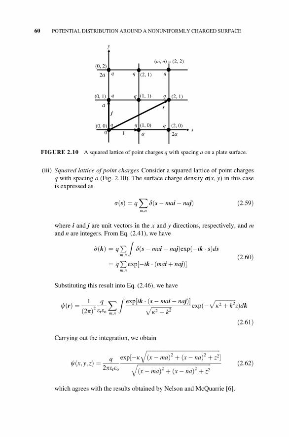
(iii) Squared lattice of point charges Consider a squared lattice of point charges

q with spacing a (Fig. 2.10). The surface charge density r(x, y) in this case

is expressed as

sðsÞ ¼ qXm;n

dðs� mai� najÞ ð2:59Þ

where i and j are unit vectors in the x and y directions, respectively, and mand n are integers. From Eq. (2.41), we have

sðkÞ ¼ qPm;n

Zdðs� mai� najÞexpð�ik � sÞds

¼ qPm;n

exp½�ik � ðmaiþ najÞ�ð2:60Þ


cðrÞ ¼ 1

ð2pÞ2q

ereo

Xm;n

Zexp½ik � ðs� mai� najÞ�ffiffiffiffiffiffiffiffiffiffiffiffiffiffiffi

k2 þ k2p expð�


pzÞdk

ð2:61Þ


cðx; y; zÞ ¼ q

2pereo

exp½�kffiffiffiffiffiffiffiffiffiffiffiffiffiffiffiffiffiffiffiffiffiffiffiffiffiffiffiffiffiffiffiffiffiffiffiffiffiffiffiffiffiffiffiffiffiffiffiffiffiffiffiffiffiffiðx� maÞ2 þ ðx� naÞ2 þ z2

q�ffiffiffiffiffiffiffiffiffiffiffiffiffiffiffiffiffiffiffiffiffiffiffiffiffiffiffiffiffiffiffiffiffiffiffiffiffiffiffiffiffiffiffiffiffiffiffiffiffiffiffiffiffiffi

ðx� maÞ2 þ ðx� naÞ2 þ z2q ð2:62Þ

which agrees with the results obtained by Nelson and McQuarrie [6].

0x

y

i

js

(m, n) = (2, 2)

(0, 1)

(2, 0)

(2, 1)

(0, 2)

(0, 0)

(1, 1)

(1, 0)

(2, 1)q

q

qqq

q q

qq

a 2a

2a

a

FIGURE 2.10 A squared lattice of point charges q with spacing a on a plate surface.


Figure 2.11 shows the potential distribution c near a plate surface carry-

ing a squared lattice of point charges q¼ e¼ 1.6� 10�19 C with spacing a¼ 2.5 nm in an aqueous 1-1 electrolyte solution of concentration 0.1M at

25C (er¼ 78.55) calculated via Eq. (2.62) at distances z¼ 0.5 nm and z¼ 1

nm. Figure 2.12 shows the potential distribution c(x, y, z) as a function of

FIGURE 2.11 Potential distribution c near a plate surface carrying a squared lattice of

point charges q= e= 1.6� 10�19 C with spacing a = 2.5 nm in an aqueous 1-1 electrolyte so-

lution of concentration 0.1M at 25C (er = 78.55) calculated via Eq. (2.62) at distances

z = 0.5 nm and z= 1 nm.

FIGURE 2.12 Potential distribution c(x, y, z) near a plate surface carrying a squared lat-

tice of point charges q= e = 1.6� 10�19 C with spacing a = 2.5 nm in an aqueous 1-1 electro-

lyte solution of concentration 0.1M at 25C (er = 78.55) as a function of the distance z fromthe plate surface at x = y= 0 and at x= y = a/2 = 1.25 nm, in comparison with the result for the

smeared charge model (dashed line).


the distance z from the plate surface at x¼ y¼ 0 and at x¼ y¼a/2¼ 1.25 nm, in comparison with the result for the smeared charge model.

We see that for distances away from the plate surface greater than the

Debye length 1/k (1 nm in this case), the electric potential due to a lattice of

point charges is essentially the same as that for the smeared charge model.

For small distances less than 1/k, however, the potential due to the array of

point charges differs significantly from that for the smeared charge model.

REFERENCES

1. B. V. Derjaguin and L. Landau, Acta Physicochim. 14 (1941) 633.

2. E. J. W. Verwey and J. Th. G. Overbeek, Theory of the Stability of Lyophobic Colloids,Elsevier, Amsterdam, 1948.

3. H. Ohshima and K. Furusawa (Eds.), Electrical Phenomena at Interfaces: Fundamentals,Measurements, and Applications, 2nd edition, revised and expanded, Dekker, New York,

1998.

4. H. Ohshima, Theory of Colloid and Interfacial Electric Phenomena, Elsevier/Academic

Press, Amsterdam, 2006.

5. H. Ohshima, Colloids Surf. B: Biointerfaces 15 (1999) 31.

6. A. P. Nelson and D. A. McQuarrie, J. Theor. Biol. 55 (1975) 13.


biophysical chemistry of biointerfaces (ohshima/biophysical chemistry of biointerfaces) || potential...

Documents