bioinformatica t3-scoring matrices

FBW

08-10-2012

Wim Van Criekinge

Inhoud Lessen: Bioinformatica

GEEN LES

Ove

rvie

w

• Introduction

– Short recap on databases

– Definitions

• Scoring Matrices

– Theoretical

– Empirial

• PAM (pam-simulator.pl)

• BLOSUM

• Pairwise alignment

– Dot-plots (dotplot-simulator.pl)

Overview

Major sites

NCBI - The National Center for Biotechnology Information

http://www.ncbi.nlm.nih.gov/

The National Center for Biotechnology Information (NCBI) at

the National Library of Medicine (NLM), a part of the National

Institutes of Health (NIH).

ExPASy - Molecular Biology Server

http://expasy.hcuge.ch/www/

Molecular biology WWW server of the Swiss Institute of

Bioinformatics (SIB). This server is dedicated to the analysis of

protein sequences and structures as well as 2-D PAGE

EBI - European Bioinformatics Institute

http://www.ebi.ac.uk/

http://www.ncbi.nlm.nih.gov/

http://expasy.hcuge.ch/www/

http://www.ebi.ac.uk/

Anno 2002 Anno 2003

Anno 2004

Anno 2005

Anno 2006

Anno 2007

Anno 2009

Anno 2010

Anno 2010

Anno 2011

Anno 2012

Ove

rvie

w

• Introduction


– Definitions


– Theoretical

– Empirial


• BLOSUM



Overview

IdentityThe extent to which two (nucleotide or amino acid)

sequences are invariant.

HomologySimilarity attributed to descent from a common ancestor.

Definitions

RBP: 26 RVKENFDKARFSGTWYAMAKKDPEGLFLQDNIVAEFSVDETGQMSATAKGRVRLLNNWD- 84

+ K ++ + + GTW++MA+ L + A V T + +L+ W+

glycodelin: 23 QTKQDLELPKLAGTWHSMAMA-TNNISLMATLKAPLRVHITSLLPTPEDNLEIVLHRWEN 81

OrthologousHomologous sequences in different species

that arose from a common ancestral gene

during speciation; may or may not be responsible

for a similar function.

ParalogousHomologous sequences within a single species

that arose by gene duplication.

Definitions

speciation

duplication

fly GAKKVIISAP SAD.APM..F VCGVNLDAYK PDMKVVSNAS CTTNCLAPLA

human GAKRVIISAP SAD.APM..F VMGVNHEKYD NSLKIISNAS CTTNCLAPLA

plant GAKKVIISAP SAD.APM..F VVGVNEHTYQ PNMDIVSNAS CTTNCLAPLA

bacterium GAKKVVMTGP SKDNTPM..F VKGANFDKY. AGQDIVSNAS CTTNCLAPLA

yeast GAKKVVITAP SS.TAPM..F VMGVNEEKYT SDLKIVSNAS CTTNCLAPLA

archaeon GADKVLISAP PKGDEPVKQL VYGVNHDEYD GE.DVVSNAS CTTNSITPVA

fly KVINDNFEIV EGLMTTVHAT TATQKTVDGP SGKLWRDGRG AAQNIIPAST

human KVIHDNFGIV EGLMTTVHAI TATQKTVDGP SGKLWRDGRG ALQNIIPAST

plant KVVHEEFGIL EGLMTTVHAT TATQKTVDGP SMKDWRGGRG ASQNIIPSST

bacterium KVINDNFGII EGLMTTVHAT TATQKTVDGP SHKDWRGGRG ASQNIIPSST

yeast KVINDAFGIE EGLMTTVHSL TATQKTVDGP SHKDWRGGRT ASGNIIPSST

archaeon KVLDEEFGIN AGQLTTVHAY TGSQNLMDGP NGKP.RRRRA AAENIIPTST

fly GAAKAVGKVI PALNGKLTGM AFRVPTPNVS VVDLTVRLGK GASYDEIKAK

human GAAKAVGKVI PELNGKLTGM AFRVPTANVS VVDLTCRLEK PAKYDDIKKV

plant GAAKAVGKVL PELNGKLTGM AFRVPTSNVS VVDLTCRLEK GASYEDVKAA

bacterium GAAKAVGKVL PELNGKLTGM AFRVPTPNVS VVDLTVRLEK AATYEQIKAA

yeast GAAKAVGKVL PELQGKLTGM AFRVPTVDVS VVDLTVKLNK ETTYDEIKKV

archaeon GAAQAATEVL PELEGKLDGM AIRVPVPNGS ITEFVVDLDD DVTESDVNAA

Multiple sequence alignment of

glyceraldehyde- 3-phsophate dehydrogenases

This power of sequence alignments

• empirical finding: if two biological sequences are sufficiently similar, almost invariably they have similar biological functions and will be descended from a common ancestor.

• (i) function is encoded into sequence, this means: the sequence provides the syntax and

• (ii) there is a redundancy in the encoding, many positions in the sequence may be changed without perceptible changes in the function, thus the semantics of the encoding is robust.

Ove

rvie

w

• Introduction


– Definitions


– Theoretical

– Empirial


• BLOSUM



Overview

A metric …

It is very important to realize, that all subsequent results depend critically on just how this is done and what model lies at the basis for the construction of a specific scoring matrix.

A scoring matrix is a tool to quantify how well a certain model is represented in the alignment of two sequences, and any result obtained by its application is meaningful exclusively in the context of that model.

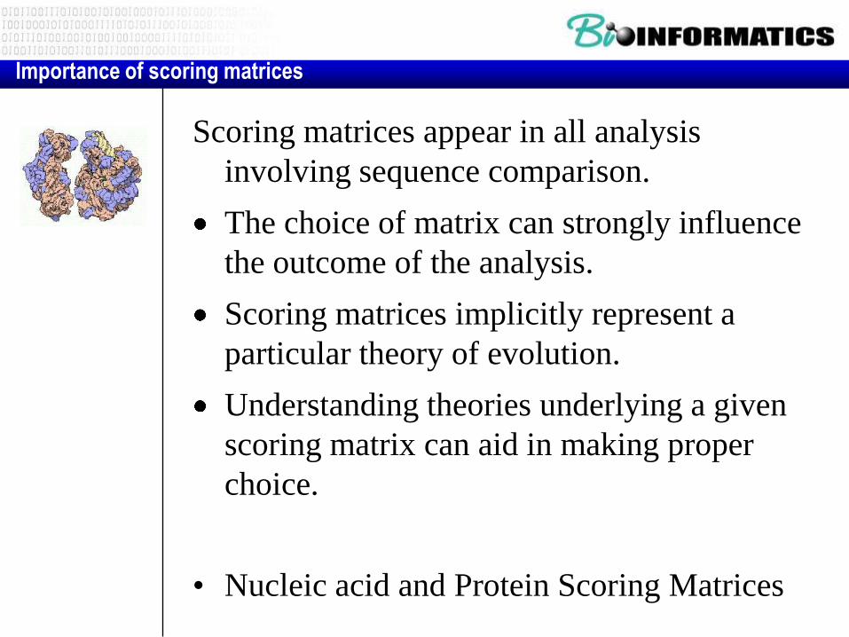
Scoring matrices appear in all analysis

involving sequence comparison.

The choice of matrix can strongly influence

the outcome of the analysis.

Scoring matrices implicitly represent a

particular theory of evolution.

Understanding theories underlying a given

scoring matrix can aid in making proper

choice.

• Nucleic acid and Protein Scoring Matrices

Importance of scoring matrices

• Identity matrix (similarity) BLAST matrix (similarity) A T C G A T C G

A 1 0 0 0 A 5 -4 -4 -4

T 0 1 0 0 T -4 5 -4 -4

C 0 0 1 0 C -4 -4 5 -4

G 0 0 0 1 G -4 -4 -4 5

• Transition/Transversion Matrix A T C G

A 0 5 5 1T 5 0 1 5C 5 1 0 5G 1 5 5 0

Nucleic Acid Scoring Matrices

G and C

purine-pyrimidine

A and T

purine -pyrimidine

• Nucleotide bases fall into two categories depending on the ring structure of the base. Purines (Adenine and Guanine) are two ring bases, pyrimidines (Cytosine and Thymine) are single ring bases. Mutations in DNA are changes in which one base is replaced by another.

• A mutation that conserves the ring number is called a transition (e.g., A -> G or C -> T) a mutation that changes the ring number are called transversions. (e.g. A -> C or A -> T and so on).

A T C G

A 0 5 5 1

T 5 0 1 5

C 5 1 0 5

G 1 5 5 0

Transition/Transversion Matrix

• Although there are more ways to create a transversion, the number of transitions observed to occur in nature (i.e., when comparing related DNA sequences) is much greater. Since the likelihood of transitions is greater, it is sometimes desireable to create a weight matrix which takes this propensity into account when comparing two DNA sequences.

• Use of a Transition/Transversion Matrix reduces noise in comparisons of distantly related sequences.

Transition/Transversion Matrix

A T C G

A 0 5 5 1

T 5 0 1 5

C 5 1 0 5

G 1 5 5 0

The Genome Chose Its Alphabet With Care

• Of all the nucleotide bases available, why did nature pick the four we know as A, T, G, and C for the genomic alphabet ?

• The choice of A, T, G, and C incorporates a tactic for minimizing the occurrence of errors in the pairing of bases, in the same way that error-coding systems are incorporated into ISBNs on books, credit card numbers, bank accounts, and airline tickets.

• In the error-coding theory first developed in 1950 by Bell Telephone Laboratories researcher Richard Hamming, a so-called parity bit is added to the end of digital numbers to make the digits add up to an even number. For example, when transmitting the number 100110, you would add an extra 1 onto the end (100110,1), and the number 100001 would have a zero added (100001,0). The most likely transmission error is a single digit changed from 1 to 0 or vice versa. Such a change would cause the sum of the digits to be odd, and the recipient of that number can assume that it was incorrectly transmitted.


• Represent each nucleotide as a four-digit binary number.

• The first three digits represent the three bonding sites that each nucleotide presents to its partner. Each site is either a hydrogen donor or acceptor; a nucleotide offering donor-acceptor-acceptor sites would be represented as 100 and would bond only with an acceptor-donor-donor nucleotide, or 011.

• The fourth digit is 1 if the nucleotide is a single-ringed pyrimidine type and 0 if it is a double-ringed purine type.

• Nucleotides readily bond with members of the other type.


• The final digit acted as a parity bit: The four digits of A, T, G, and C all add up to an even number.

• Nature restricted its choice to nucleotides of even parity because "alphabets composed of nucleotides of mixed parity would have catastrophic error rates.

• For example, nucleotide C (100,1) binds naturally to nucleotide G (011,0), but it might accidentally bind to the odd parity nucleotide X (010,0), because there is just one mismatch. Such a bond would be weak compared to C-G but not impossible. However, C is highly unlikely to bond to any other even-parity nucleotides, such as the idealized amino-adenine (101,0), because there are two mismatches

• So, nature has avoided such mistakes by banishing all odd-parity nucleotides from the DNA alphabet.


• The simplest metric in use is the

identity metric.

• If two amino acids are the same,

they are given one score, if they are

not, they are given a different score -

regardless, of what the replacement

is.

• One may give a score of 1 for

matches and 0 for mismatches - this

leads to the frequently used unitary

matrix

Protein Scoring Matrices: Unitary Matrix


A R N D C Q E G H I L K M F P S T W Y V

A 1 0 0 0 0 0 0 0 0 0 0 0 0 0 0 0 0 0 0 0

R 0 1 0 0 0 0 0 0 0 0 0 0 0 0 0 0 0 0 0 0

N 0 0 1 0 0 0 0 0 0 0 0 0 0 0 0 0 0 0 0 0

D 0 0 0 1 0 0 0 0 0 0 0 0 0 0 0 0 0 0 0 0

C 0 0 0 0 1 0 0 0 0 0 0 0 0 0 0 0 0 0 0 0

Q 0 0 0 0 0 1 0 0 0 0 0 0 0 0 0 0 0 0 0 0

E 0 0 0 0 0 0 1 0 0 0 0 0 0 0 0 0 0 0 0 0

G 0 0 0 0 0 0 0 1 0 0 0 0 0 0 0 0 0 0 0 0

H 0 0 0 0 0 0 0 0 1 0 0 0 0 0 0 0 0 0 0 0

I 0 0 0 0 0 0 0 0 0 1 0 0 0 0 0 0 0 0 0 0

L 0 0 0 0 0 0 0 0 0 0 1 0 0 0 0 0 0 0 0 0

K 0 0 0 0 0 0 0 0 0 0 0 1 0 0 0 0 0 0 0 0

M 0 0 0 0 0 0 0 0 0 0 0 0 1 0 0 0 0 0 0 0

F 0 0 0 0 0 0 0 0 0 0 0 0 0 1 0 0 0 0 0 0

P 0 0 0 0 0 0 0 0 0 0 0 0 0 0 1 0 0 0 0 0

S 0 0 0 0 0 0 0 0 0 0 0 0 0 0 0 1 0 0 0 0

T 0 0 0 0 0 0 0 0 0 0 0 0 0 0 0 0 1 0 0 0

W 0 0 0 0 0 0 0 0 0 0 0 0 0 0 0 0 0 1 0 0

Y 0 0 0 0 0 0 0 0 0 0 0 0 0 0 0 0 0 0 1 0

V 0 0 0 0 0 0 0 0 0 0 0 0 0 0 0 0 0 0 0 1


• The simplest matrix:

– High scores for Identities

– Low scores for non-identities

• Works for closely related proteins

• Or one could assign +6 for a match and -1 for a mismatch, this would be a matrix useful for local alignment procedures, where a negative expectation value for randomly aligned sequences is required to ensure that the score will not grow simply from extending the alignment in a random way.

A very crude model of an evolutionary

relationship could be implemented in a

scoring matrix in the following way: since

all point-mutations arise from nucleotide

changes, the probability that an observed

amino acid pair is related by chance,

rather than inheritance should depend on

the number of point mutations necessary

to transform one codon into the other.

A metric resulting from this model would

define the distance between two amino

acids by the minimal number of nucleotide

changes required.

Genetic Code Matrix

A S G L K V T P E D N I Q R F Y C H M W Z B X

Ala = A O 1 1 2 2 1 1 1 1 1 2 2 2 2 2 2 2 2 2 2 2 2 2

Ser = S 1 O 1 1 2 2 1 1 2 2 1 1 2 1 1 1 1 2 2 1 2 2 2

Gly = G 1 1 0 2 2 1 2 2 1 1 2 2 2 1 2 2 1 2 2 1 2 2 2

Leu = L 2 1 2 0 2 1 2 1 2 2 2 1 1 1 1 2 2 1 1 1 2 2 2

Lys = K 2 2 2 2 0 2 1 2 1 2 1 1 1 1 2 2 2 2 1 2 1 2 2

Val = V 1 2 1 1 2 0 2 2 1 1 2 1 2 2 1 2 2 2 1 2 2 2 2

Thr = T 1 1 2 2 1 2 0 1 2 2 1 1 2 1 2 2 2 2 1 2 2 2 2

Pro = P 1 1 2 1 2 2 1 0 2 2 2 2 1 1 2 2 2 1 2 2 2 2 2

Glu - E 1 2 1 2 1 1 2 2 0 1 2 2 1 2 2 2 2 2 2 2 1 2 2

Asp = D 1 2 1 2 2 1 2 2 1 O 1 2 2 2 2 1 2 1 2 2 2 1 2

Asn = N 2 1 2 2 1 2 1 2 2 1 O 1 2 2 2 1 2 1 2 2 2 1 2

Ile = I 2 1 2 1 1 1 1 2 2 2 1 0 2 1 1 2 2 2 1 2 2 2 2

Gln = Q 2 2 2 1 1 2 2 1 1 2 2 2 0 1 2 2 2 1 2 2 1 2 2

Arg = R 2 1 1 1 1 2 1 1 2 2 2 1 1 0 2 2 1 1 1 1 2 2 2

Phe = F 2 1 2 1 2 1 2 2 2 2 2 1 2 2 0 1 1 2 2 2 2 2 2

Tyr = Y 2 1 2 2 2 2 2 2 2 1 1 2 2 2 1 O 1 1 3 2 2 1 2

Cys = C 2 1 1 2 2 2 2 2 2 2 2 2 2 1 1 1 0 2 2 1 2 2 2

His = H 2 2 2 1 2 2 2 1 2 1 1 2 1 1 2 1 2 0 2 2 2 1 2

Met = M 2 2 2 1 1 1 1 2 2 2 2 1 2 1 2 3 2 2 0 2 2 2 2

Trp = W 2 1 1 1 2 2 2 2 2 2 2 2 2 1 2 2 1 2 2 0 2 2 2

Glx = Z 2 2 2 2 1 2 2 2 1 2 2 2 1 2 2 2 2 2 2 2 1 2 2

Asx = B 2 2 2 2 2 2 2 2 2 1 1 2 2 2 2 1 2 1 2 2 2 1 2

??? = X 2 2 2 2 2 2 2 2 2 2 2 2 2 2 2 2 2 2 2 2 2 2 2

The table is generated by calculating the minimum number of base changes required to

convert an amino acid in row i to an amino acid in column j.

Note Met->Tyr is the only change that requires all 3 codon positions to change.

Genetic Code Matrix

This genetic code matrix already

improves sensitivity and specificity

of alignments from the identity

matrix.

The fact that the genetic code matrix

works to align related proteins, in

the same way that matrices derived

from amino-acid properties work

says something very interesting

about the genetic code: namely that

it appears to have evolved to

minimize the effects of point

mutations.

Genetic Code Matrix

Genetic Code Matrix

• Simple identity, which scores only identical amino

acids as a match.

• Genetic code changes, which scores the

minimum number of nucieotide changes to change

a codon for one amino acid into a codon for the

other.

• Chemical similarity of amino acid side chains,

which scores as a match two amino acids which

have a similar side chain, such as hydrophobic,

charged and polar amino acid groups.

Overview

All proteins are polymers of the 20 naturally occuring amino acids. They are listed here along with their

abbreviations :-Alanine Ala A

Cysteine Cys C

Aspartic AciD Asp D

Glutamic Acid Glu E

Phenylalanine Phe F

Glycine Gly G

Histidine His H

Isoleucine Ile I

Lysine Lys K

Leucine Leu L

Methionine Met M

AsparagiNe Asn N

Proline Pro P

Glutamine Gln Q

ARginine Arg R

Serine Ser S

Threonine Thr T

Valine Val V

Tryptophan Trp W

TYrosine Tyr Y

Amino Acid Residues

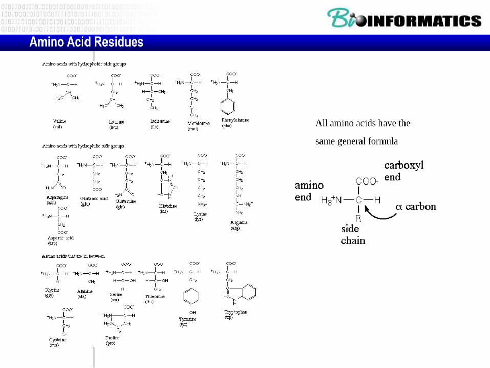
All amino acids have the

same general formula

Amino Acid Residues

• Hydrophobic-aliphatic amino acids: Their side chains consist of non-polar methyl- or methylene-groups.

– These amino acids are usually located on the interior of the protein as they are hydrophobic in nature.

– All except for alanine are bifurcated. In the cases of Val and Ile the bifurcation is close to the main chain and can therefore restrict the conformation of the polypeptide by steric hindrance.

– red and blue atoms represent polar main chain groups

Amino Acid Residues

Amino Acid Residues

• Hydrophobic-aromatic: Only

phenylalanine is entirely non-polar.

Tyrosine's phenolic side chain has a

hydroxyl substituent and tryptophan

has a nitrogen atom in its indole ring

sytem.

– These residues are nearly always found

to be largely buried in the hydrophobic

interior of a proteins as they are

prdeominantly non-polar in nature.

– However, the polar atoms of tyrosine

and tryptophan allow hydrogen bonding

interactions to be made with other

residues or even solvent molecules

Amino Acid Residues

Amino Acid Residues

Neutral-polar side chains: a number of

small aliphatic side chains containing polar

groups which cannot ionize readily.

– Serine and threonine possess hydroxyl groups in

their side chains and as these polar groups are

close to the main chain they can form hydrogen

bonds with it. This can influence the local

conformation of the polypeptide,

– Residues such as serine and asparagine are

known to adopt conformations which most other

amino acids cannot.

– The amino acids asparagine and glutamine

posses amide groups in their side chains which

are usually hydrogen-bonded whenever they

occur in the interior of a protein.

Amino Acid Residues

Amino Acid Residues

• Acidic amino acids: Aspartate and glutamate have carboxyl side chains and are therefore negatively charged at physiological pH (around neutral).

– The strongly polar nature of these residues means that they are most often found on the surface of globular proteins where they can interact favourably with solvent molecules.

– These residues can also take part in electrostatic interactions with positively charged basic amino acids.

– Aspartate and glutamate also can take on catalytic roles in the active sites of enzymes and are well known for their metal ion binding abilities

Amino Acid Residues

Amino Acid Residues

• Basic amino acids:

– histidine has the lowest pKa (around 6) and is

therefore neutral at around physiological pH.

• This amino acid occurs very frequently in enzyme

active sites as it can function as a very efficient

general acid-base catalyst.

• It also acts as a metal ion ligand in numerous

protein families.

– Lysine and arginine are more strongly basic and

are positively charged at physiological pH's. They

are generally solvated but do occasionally occur

in the interior of a protein where they are usually

involved in electrostatic interactions with

negatively charged groups such as Asp or Glu.

• Lys and Arg have important roles in anion-binding

proteins as they can interact electrostatically with

the ligand.

Amino Acid Residues

Amino Acid Residues

Conformationally important residues: Glycine and

proline are unique amino acids. They appear to

influence the conformation of the polypeptide.

• Glycine essentially lacks a side chain and therefore

can adopt conformations which are sterically

forbidden for other amino acids. This confers a high

degree of local flexibility on the polypeptide.

– Accordingly, glycine residues are frequently found in

turn regions of proteins where the backbone has to

make a sharp turn.

– Glycine occurs abundantly in certain fibrous proteins

due to its flexibility and because its small size allows

adjacent polypeptide chains to pack together closely.

• In contrast, proline is the most rigid of the twenty

naturally occurring amino acids since its side chain

is covalently linked with the main chain nitrogen

Amino Acid Residues

Amino Acid Residues

Here is one list where amino acids are grouped according to the characteristics of the side chains:

Aliphatic - alanine, glycine, isoleucine, leucine, proline, valine,

Aromatic - phenylalanine, tryptophan, tyrosine,

Acidic - aspartic acid, glutamic acid,

Basic - arginine, histidine, lysine,

Hydroxylic - serine, threonine

Sulphur-containing - cysteine, methionine

Amidic (containing amide group) -asparagine, glutamine

Amino Acid Residues

R K D E B Z S N Q G X T H A C M P V L I Y F W

Arg = R 10 10 9 9 8 8 6 6 6 5 5 5 5 5 4 3 3 3 3 3 2 1 0

Lys = K 10 10 9 9 8 8 6 6 6 5 5 5 5 5 4 3 3 3 3 3 2 1 0

Asp = D 9 9 10 10 8 8 7 6 6 6 5 5 5 5 5 4 4 4 3 3 3 2 1

Glu = E 9 9 10 10 8 8 7 6 6 6 5 5 5 5 5 4 4 4 3 3 3 2 1

Asx = B 8 8 8 8 10 10 8 8 8 8 7 7 7 7 6 6 6 5 5 5 4 4 3

Glx = Z 8 8 8 8 10 10 8 8 8 8 7 7 7 7 6 6 6 5 5 5 4 4 3

Ser = S 6 6 7 7 8 8 10 10 10 10 9 9 9 9 8 8 7 7 7 7 6 6 4

Asn = N 6 6 6 6 8 8 10 10 10 10 9 9 9 9 8 8 8 7 7 7 6 6 4

Gln = Q 6 6 6 6 8 8 10 10 10 10 9 9 9 9 8 8 8 7 7 7 6 6 4

Gly = G 5 5 6 6 8 8 10 10 10 10 9 9 9 9 8 8 8 8 7 7 6 6 5

??? = X 5 5 5 5 7 7 9 9 9 9 10 10 10 10 9 9 8 8 8 8 7 7 5

Thr = T 5 5 5 5 7 7 9 9 9 9 10 10 10 10 9 9 8 8 8 8 7 7 5

His = H 5 5 5 5 7 7 9 9 9 9 10 10 10 10 9 9 9 8 8 8 7 7 5

Ala = A 5 5 5 5 7 7 9 9 9 9 10 10 10 10 9 9 9 8 8 8 7 7 5

Cys = C 4 4 5 5 6 6 8 8 8 8 9 9 9 9 10 10 9 9 9 9 8 8 5

Met = M 3 3 4 4 6 6 8 8 8 8 9 9 9 9 10 10 10 10 9 9 8 8 7

Pro = P 3 3 4 4 6 6 7 8 8 8 8 8 9 9 9 10 10 10 9 9 9 8 7

Val = V 3 3 4 4 5 5 7 7 7 8 8 8 8 8 9 10 10 10 10 10 9 8 7

Leu = L 3 3 3 3 5 5 7 7 7 7 8 8 8 8 9 9 9 10 10 10 9 9 8

Ile = I 3 3 3 3 5 5 7 7 7 7 8 8 8 8 9 9 9 10 10 10 9 9 8

Tyr = Y 2 2 3 3 4 4 6 6 6 6 7 7 7 7 8 8 9 9 9 9 10 10 8

Phe = F 1 1 2 2 4 4 6 6 6 6 7 7 7 7 8 8 8 8 9 9 10 10 9

Trp = W 0 0 1 1 3 3 4 4 4 5 5 5 5 5 6 7 7 7 8 8 8 9 10

Hydrophobicity matrix

•Physical/Chemical characteristics: Attempt to quantify some physical or chemical attribute of

•the residues and arbitrarily assign weights based on similarities of the residues in this chosen property.

Other similarity scoring matrices might be constructed from

any property of amino acids that can be quantified

- partition coefficients between hydrophobic and hydrophilic phases

- charge

- molecular volume

Unfortunately, …

AAindex

Amino acid indices and similarity matrices (http://www.genome.ad.jp/dbget/aaindex.html)

List of 494 Amino Acid Indices in AAindex ver.6.0

• ANDN920101 alpha-CH chemical shifts (Andersen et al., 1992)

• ARGP820101 Hydrophobicity index (Argos et al., 1982)

• ARGP820102 Signal sequence helical potential (Argos et al., 1982)

• ARGP820103 Membrane-buried preference parameters (Argos et al., 1982)

• BEGF750101 Conformational parameter of inner helix (Beghin-Dirkx, 1975)

• BEGF750102 Conformational parameter of beta-structure (Beghin-Dirkx, 1975)

• BEGF750103 Conformational parameter of beta-turn (Beghin-Dirkx, 1975)

• BHAR880101 Average flexibility indices (Bhaskaran-Ponnuswamy, 1988)

• BIGC670101 Residue volume (Bigelow, 1967)

• BIOV880101 Information value for accessibility; average fraction 35% (Biou et al., 1988)

• BIOV880102 Information value for accessibility; average fraction 23% (Biou et al., 1988)

• BROC820101 Retention coefficient in TFA (Browne et al., 1982)

• BROC820102 Retention coefficient in HFBA (Browne et al., 1982)

• BULH740101 Transfer free energy to surface (Bull-Breese, 1974)

• BULH740102 Apparent partial specific volume (Bull-Breese, 1974)

http://www.genome.ad.jp/dbget/aaindex.html

Protein Eng. 1996 Jan;9(1):27-36.

• Simple identity, which scores only identical amino

acids as a match.

• Genetic code changes, which scores the

minimum number of nucieotide changes to change

a codon for one amino acid into a codon for the

other.

• Chemical similarity of amino acid side chains,

which scores as a match two amino acids which

have a similar side chain, such as hydrophobic,

charged and polar amino acid groups.

• The Dayhoff percent accepted mutation (PAM)

family of matrices, which scores amino acid pairs

on the basis of the expected frequency of

substitution of one amino acid for the other during

protein evolution.

Overview

• In the absence of a valid model derived from first principles, an empirical approachseems more appropriate to score amino acid similarity.

• This approach is based on the assumption that once the evolutionary relationship of two sequences is established, the residues that did exchange are similar.

Dayhoff Matrix

Model of Evolution:

“Proteins evolve through a succesion of

independent point mutations, that are

accepted in a population and

subsequently can be observed in the

sequence pool.”

Definition:

The evolutionary distance between two

sequences is the (minimal) number of

point mutations that was necessary to

evolve one sequence into the other

Overview

• The model used here states that

proteins evolve through a succesion of

independent point mutations, that are

accepted in a population and

subsequently can be observed in the

sequence pool.

• We can define an evolutionary

distance between two sequences as

the number of point mutations that was

necessary to evolve one sequence into

the other.

Principle

• M.O. Dayhoff and colleagues

introduced the term "accepted point

mutation" for a mutation that is stably

fixed in the gene pool in the course

of evolution. Thus a measure of

evolutionary distance between two

sequences can be defined:

• A PAM (Percent accepted mutation)

is one accepted point mutation on

the path between two sequences,

per 100 residues.

Overview

First step: finding “accepted mutations”

In order to identify accepted point

mutations, a complete phylogenetic

tree including all ancestral sequences

has to be constructed. To avoid a

large degree of ambiguities in this

step, Dayhoff and colleagues

restricted their analysis to sequence

families with more than 85% identity.

Principles of Scoring Matrix Construction

Identification of accepted point mutations:

•Collection of correct (manual) alignments

• 1300 sequences in 72 families

• closely related in order not to get multiply

changes at the same position

• Construct a complete phylogenetic tree including all

ancestral sequences.

• Dayhoff et al restricted their analysis to

sequence families with more than 85%

identity.

• Tabulate into a 20x20 matrix the amino acid pair

exchanges for each of the observed and inferred

sequences.

Overview

ACGH DBGH ADIJ CBIJ

\ / \ /

\ / \ /

B - C \ / A - D B - D \ / A - C

\ / \ /

\/ \/

ABGH ABIJ

\ /

\ I - G /

\ J - H /

\ /

\ /

|

|

|

Overview

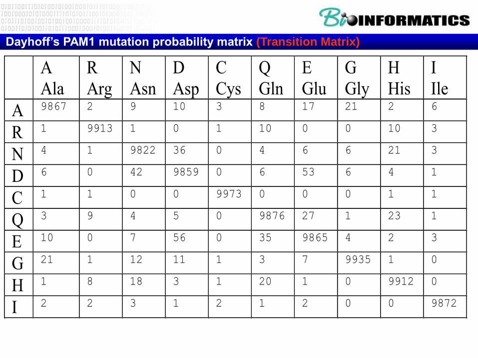
Dayhoff’s PAM1 mutation probability matrix (Transition Matrix)

A

Ala

R

Arg

N

Asn

D

Asp

C

Cys

Q

Gln

E

Glu

G

Gly

H

His

I

Ile

A 9867 2 9 10 3 8 17 21 2 6

R 1 9913 1 0 1 10 0 0 10 3

N 4 1 9822 36 0 4 6 6 21 3

D 6 0 42 9859 0 6 53 6 4 1

C 1 1 0 0 9973 0 0 0 1 1

Q 3 9 4 5 0 9876 27 1 23 1

E 10 0 7 56 0 35 9865 4 2 3

G 21 1 12 11 1 3 7 9935 1 0

H 1 8 18 3 1 20 1 0 9912 0

I 2 2 3 1 2 1 2 0 0 9872

PAM1: Transition Matrix

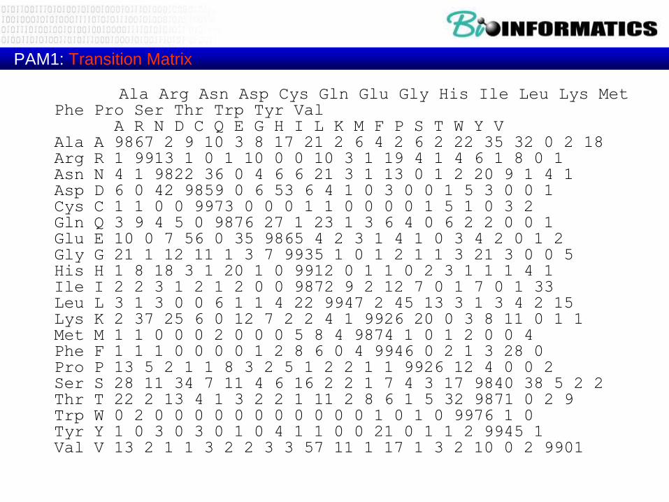
Ala Arg Asn Asp Cys Gln Glu Gly His Ile Leu Lys Met Phe Pro Ser Thr Trp Tyr Val

A R N D C Q E G H I L K M F P S T W Y VAla A 9867 2 9 10 3 8 17 21 2 6 4 2 6 2 22 35 32 0 2 18Arg R 1 9913 1 0 1 10 0 0 10 3 1 19 4 1 4 6 1 8 0 1Asn N 4 1 9822 36 0 4 6 6 21 3 1 13 0 1 2 20 9 1 4 1Asp D 6 0 42 9859 0 6 53 6 4 1 0 3 0 0 1 5 3 0 0 1Cys C 1 1 0 0 9973 0 0 0 1 1 0 0 0 0 1 5 1 0 3 2Gln Q 3 9 4 5 0 9876 27 1 23 1 3 6 4 0 6 2 2 0 0 1Glu E 10 0 7 56 0 35 9865 4 2 3 1 4 1 0 3 4 2 0 1 2Gly G 21 1 12 11 1 3 7 9935 1 0 1 2 1 1 3 21 3 0 0 5His H 1 8 18 3 1 20 1 0 9912 0 1 1 0 2 3 1 1 1 4 1Ile I 2 2 3 1 2 1 2 0 0 9872 9 2 12 7 0 1 7 0 1 33Leu L 3 1 3 0 0 6 1 1 4 22 9947 2 45 13 3 1 3 4 2 15Lys K 2 37 25 6 0 12 7 2 2 4 1 9926 20 0 3 8 11 0 1 1Met M 1 1 0 0 0 2 0 0 0 5 8 4 9874 1 0 1 2 0 0 4Phe F 1 1 1 0 0 0 0 1 2 8 6 0 4 9946 0 2 1 3 28 0Pro P 13 5 2 1 1 8 3 2 5 1 2 2 1 1 9926 12 4 0 0 2Ser S 28 11 34 7 11 4 6 16 2 2 1 7 4 3 17 9840 38 5 2 2Thr T 22 2 13 4 1 3 2 2 1 11 2 8 6 1 5 32 9871 0 2 9Trp W 0 2 0 0 0 0 0 0 0 0 0 0 0 1 0 1 0 9976 1 0Tyr Y 1 0 3 0 3 0 1 0 4 1 1 0 0 21 0 1 1 2 9945 1Val V 13 2 1 1 3 2 2 3 3 57 11 1 17 1 3 2 10 0 2 9901

Numbers of accepted point mutations (x10)

accumulated from closely related

sequences.

Fractional exchanges result when ancestral

sequences are ambiguous: the

probabilities are distributed equally

among all possibilities.

The total number of exchanges tallied was

1,572. Note that 36 exchanges were

never observed.

The Asp-Glu pair had the largest number of

exchanges

PAM1: Transition Matrix

Second step: Frequencies of Occurence

If the properties of amino acids differ and if

they occur with different frequencies, all

statements we can make about the average

properties of sequences will depend on the

frequencies of occurence of the individual

amino acids. These frequencies of

occurence are approximated by the

frequencies of observation. They are the

number of occurences of a given amino acid

divided by the number of amino-acids

observed.

The sum of all is one.


Amino acid frequencies

1978 1991

L 0.085 0.091

A 0.087 0.077

G 0.089 0.074

S 0.070 0.069

V 0.065 0.066

E 0.050 0.062

T 0.058 0.059

K 0.081 0.059

I 0.037 0.053

D 0.047 0.052

R 0.041 0.051

P 0.051 0.051

N 0.040 0.043

Q 0.038 0.041

F 0.040 0.040

Y 0.030 0.032

M 0.015 0.024

H 0.034 0.023

C 0.033 0.020

W 0.010 0.014

Second step: Frequencies of Occurence

Third step: Relative Mutabilities

• To obtain a complete picture of the mutational process, the amino-acids that do not mutate must be taken into account too.

• We need to know: what is the chance, on average, that a given amino acid will mutate at all. This is the relative mutability of the amino acid.

• It is obtained by multiplying the number of observed changes by the amino acids frequency of occurence.


Compute amino acid mutability, mj, i.e., the propability

of a given amino acid, j, to be replaced.

Aligned A D A

Sequences A D B

Amino Acids A B D

Observed Changes 1 1 0

Frequency of Occurence 3 1 2

(Total Composition)

Relative Mutability .33 1 0

Overview

1978 1991A 100 100C 20 44D 106 86E 102 77F 41 51G 49 50H 66 91I 96 103K 56 72L 40 54M 94 93N 134 104P 56 58Q 93 84R 65 83S 120 117T 97 107V 74 98W 18 25Y 41 50


Fourth step: Mutation Probability Matrix

• With these data the probability that an amino acid in

row i of the matrix will replace the amino acid in

column j can be calculated: it is the mutability of amino

acid j, multiplied by the relative pair exchange

frequency (the pair exchange frequency for ij divided

by the sum of all pair exchange frequencies for amino

acid i).

Mij= The mutation probability matrix gives the

probability, that an amino acid i will replace an amino

acid of type j in a given evolutionary interval, in two

related sequences


ADB

ADA

A D B

A

D

B

i

j

Fifth step: The Evolutionary Distance

• Since the represent the probabilites

for amino acids to remain

conserved, if we scale all cells of our

matrix by a constant factor we can

scale the matrix to reflect a specific

overall probability of change. We

may chose so that the expected

number of changes is 1 %, this

gives the matrix for the evolutionary

distance of 1 PAM.


6. Relatedness Odds

• By comparison, the probability that

that same event is observed by

random chance is simply given by

the frequency of occurence of

amino acid i

• Rij = probability that j replaces i in

related proteins

• Piran = probability that j replaces I by

chance (eg unrelated proteins)

• Piran = fi = the frequency of

occurance of amino acid i


Last step: the log-odds matrix• Since multiplication is a computationally

expensive process, it is preferrable to add

the logarithms of the matrix elements. This

matrix, the log odds matrix, is the

foundation of quantitative sequence

comparisons under an evolutionary model.

• Since the Dayhoff matrix was taken as the

log to base 10, a value of +1 would mean

that the corresponding pair has been

observed 10 times more frequently than

expected by chance. A value of -0.2 would

mean that the observed pair was observed

1.6 times less frequently than chance

would predict.


• http://www.bio.brandeis.edu/InterpGenes/Proj

ect/align12.htm

http://www.bio.brandeis.edu/InterpGenes/Project/align12.htm

http://www.bio.brandeis.edu/InterpGenes/Project/align12.htm

A B C D E F G H I K L M N P Q R S T V W Y Z

0.4 0.0 -0.4 0.0 0.0 -0.8 0.2 -0.2 -0.2 -0.2 -0.4 -0.2 0.0 0.2 0.0 -0.4 0.2 0.2 0.0 -1.2 -0.6 0.0 A

0.5 -0.9 0.6 0.4 -1.0 0.1 0.3 -0.4 0.1 -0.7 -0.5 0.4 -0.2 0.3 -0.1 0.1 0.0 -0.4 -1.1 -0.6 0.4 B

2.4 -1.0 -1.0 -0.8 -0.6 -0.6 -0.4 -1.0 -1.2 -1.0 -0.8 -0.6 -1.0 -0.8 0.0 -0.4 -0.4 -1.6 0.0 -1.0 C

0.8 0.6 -1.2 0.2 0.2 -0.4 0.0 -0.8 -0.6 0.4 -0.2 0.4 -0.2 0.0 0.0 -0.4 -1.4 -0.8 0.5 D

0.8 -1.0 0.0 0.2 -0.4 0.0 -0.6 -0.4 0.2 -0.2 0.4 -0.2 0.0 0.0 -0.4 -1.4 -0.8 0.6 E

1.8 -1.0 -0.4 0.2 -1.0 0.4 0.0 -0.8 -1.0 -1.0 -0.8 -0.6 -0.6 -0.2 0.0 1.4 -1.0 F

1.0 -0.4 -0.6 -0.4 -0.8 -0.6 0.0 -0.2 -0.2 -0.6 0.2 0.0 -0.2 -1.4 -1.0 -0.1 G

1.2 -0.4 0.0 -0.4 -0.4 0.4 0.0 0.6 0.4 -0.2 -0.2 -0.4 -0.6 0.0 -0.4 H

1.0 -0.4 0.4 0.4 -0.4 -0.4 -0.4 -0.4 -0.2 0.0 0.8 -1.0 -0.2 -0.4 I

1.0 -0.6 0.0 0.2 -0.2 0.2 0.6 0.0 0.0 -0.4 -0.6 -0.8 0.1 K

1.2 0.8 -0.6 -0.6 -0.4 -0.6 -0.6 -0.4 0.4 -0.4 -0.2 -0.5 L

1.2 -0.4 -0.4 -0.2 0.0 -0.4 -0.2 0.4 -0.8 -0.4 -0.3 M

0.4 -0.2 0.2 0.0 0.2 0.0 -0.4 -0.8 -0.4 0.2 N

1.2 0.0 0.0 0.2 0.0 -0.2 -1.2 -1.0 -0.1 P

0.8 0.2 -0.2 -0.2 -0.4 -1.0 -0.8 0.6 Q

1.2 0.0 -0.2 -0.4 0.4 -0.8 0.6 R

0.4 0.2 -0.2 -0.4 -0.6 -0.1 S

0.6 0.0 -1.0 -0.6 -0.1 T

0.8 -1.2 -0.4 -0.4 V

3.4 0.0 -1.2 W

2.0 -0.8 Y

0.6 Z

PAM 1 Scoring Matrix

• Some of the properties go into the makeup of PAM matrices are - amino acid residue size, shape, local concentrations of electric charge, van der Waals surface, ability to form salt bridges, hydrophobic interactions, and hydrogen bonds. – These patterns are imposed principally

by natural selection and only secondarily by the constraints of the genetic code.

– Coming up with one’s own matrix of weights based on some logical features may not be very successful because your logical features may have been over-written by other more important considerations.

Overview

• Two aspects of this process cause the

evolutionary distance to be unequal in

general to the number of observed

differences between the sequences:

– First, there is a chance that a certain

residue may have mutated, than reverted,

hiding the effect of the mutation.

– Second, specific residues may have

mutated more than once, thus the number

of point mutations is likely to be larger

than the number of differences between

the two sequences..


Similarity ve. distance

• Initialize:

– Generate Random protein (1000 aa)

• Simulate evolution (eg 250 for PAM250)

– Apply PAM1 Transition matrix to each amino

acid

– Use Weighted Random Selection

• Iterate

– Measure difference to orginal protein

Experiment: pam-simulator.pl

Dayhoff’s PAM1 mutation probability matrix (Transition Matrix)

A

Ala

R

Arg

N

Asn

D

Asp

C

Cys

Q

Gln

E

Glu

G

Gly

H

His

I

Ile

A 9867 2 9 10 3 8 17 21 2 6

R 1 9913 1 0 1 10 0 0 10 3

N 4 1 9822 36 0 4 6 6 21 3

D 6 0 42 9859 0 6 53 6 4 1

C 1 1 0 0 9973 0 0 0 1 1

Q 3 9 4 5 0 9876 27 1 23 1

E 10 0 7 56 0 35 9865 4 2 3

G 21 1 12 11 1 3 7 9935 1 0

H 1 8 18 3 1 20 1 0 9912 0

I 2 2 3 1 2 1 2 0 0 9872

Weighted Random Selection

• Ala => Xxx (%)

A

R

N

D

C

Q

E

G

H

I

L

K

M

F

P

S

T

W

Y

V

PAM-Simulator

PAM-simulator

0

20

40

60

80

100

120

0 50 100 150 200 250 300

PAM

%id

en

tity

PAM-Simulator

PAM-Simulator

0

10

20

30

40

50

60

70

80

90

100

0 200 400 600 800 1000 1200 1400 1600 1800 2000

PAM

% i

den

tity

PAM Value Distance(%)

80 50

100 60

200 75

250 85 <- Twilight zone

300 92

(From Doolittle, 1987, Of URFs and ORFs,

University Science Books)

Some PAM values and their corresponding observed distances

•When the PAM distance value between two distantly related proteins nears the value 250 it becomes difficult to tell whether the two proteins are homologous, or that they are two at randomly taken proteins that can be aligned by chance. In that case we speak of the 'twilight zone'.

•The relation between the observed percentage in distance of two sequences versus PAM value. Two randomly diverging sequences change in a negatively exponential fashion. After the insertion of gaps to two random sequences, it can be expected that they will be 80 - 90 % dissimilar (from Doolittle, 1987 ).

• Creation of a pam series from evolutionary

simulations

• pam2=pam1^2

• pam3=pam1^3

• And so on…

• pam30,60,90,120,250,300

• low pam - closely related sequences

– high scores for identity and low scores for

substitutions - closer to the identity matrix

• high pam - distant sequences

– at pam2000 all information is degenerate except

for cysteins

• pam250 is the most popular and general

– one amino acid in five remains unchanged

(mutability varies among the amino acids)

Overview

250 PAM evolutionary distance

A R N D C Q E G H I L K M F P

Ala A 13 6 9 9 5 8 9 12 6 8 6 7 7 4 11Arg R 3 17 4 3 2 5 3 2 6 3 2 9 4 1 4 Asn N 4 4 6 7 2 5 6 4 6 3 2 5 3 2 4Asp D 5 4 8 11 1 7 10 5 6 3 2 5 3 1 4 Cys C 2 1 1 1 52 1 1 2 2 2 1 1 1 1 2Gln Q 3 5 5 6 1 10 7 3 7 2 3 5 3 1 4Glu E 5 4 7 11 1 9 12 5 6 3 2 5 3 1 4Gly G 12 5 10 10 4 7 9 27 5 5 4 6 5 3 8 His H 2 5 5 4 2 7 4 2 15 2 2 3 2 2 3 Ile I 3 2 2 2 2 2 2 2 2 10 6 2 6 5 2 Leu L 6 4 4 3 2 6 4 3 5 15 34 4 20 13 5 Lys K 6 18 10 8 2 10 8 5 8 5 4 24 9 2 6 Met M 1 1 1 1 0 1 1 1 1 2 3 2 6 2 1 Phe F 2 1 2 1 1 1 1 1 3 5 6 1 4 32 1 Pro P 7 5 5 4 3 5 4 5 5 3 3 4 3 2 20 Ser S 9 6 8 7 7 6 7 9 6 5 4 7 5 3 9 Thr T 8 5 6 6 4 5 5 6 4 6 4 6 5 3 6 Trp W 0 2 0 0 0 0 0 0 1 0 1 0 0 1 0 Tyr Y 1 1 2 1 3 1 1 1 3 2 2 1 2 15 1 Val V 7 4 4 4 4 4 4 4 5 4 15 10 4 10 5[column on left represents the replacement amino acid]

Mutation probability matrix for the evolutionary distance of 250 PAMs. To simplify the appearance, the elements are shown multiplied by 100.

In comparing two sequences of average amino acid frequency at this evolutionary distance, there is a 13% probability that a position containing Ala in the first sequence will contain Ala in the second. There is a 3% chance that it will contain Arg, and so forth.

Overview

4 3 2 1 0

A brief history of time (BYA)

Origin of

life

Origin of

eukaryotes insectsFungi/animal

Plant/animal

Earliest

fossils

BYA

Margaret Dayhoff’s 34 protein superfamilies

Protein PAMs per 100 million years

Ig kappa chain 37

Kappa casein 33

Lactalbumin 27

Hemoglobin 12

Myoglobin 8.9

Insulin 4.4

Histone H4 0.10

Ubiquitin 0.00

Many sequences depart from average composition.

Rare replacements were observed too infrequently to resolve relative probabilities accurately (for 36 pairs no replacements were observed!).

Errors in 1PAM are magnified in the extrapolation to 250PAM.

Distantly related sequences usually have islands (blocks) of conserved residues. This implies that replacement is not equally probable over entire sequence.

Sources of error

• Simple identity, which scores only identical amino acids as a match.

• Genetic code changes, which scores the minimum number of nucieotide changes to change a codon for one amino acid into a codon for the other.

• Chemical similarity of amino acid side chains, which scores as a match two amino acids which have a similar side chain, such as hydrophobic, charged and polar amino acid groups.

• The Dayhoff percent accepted mutation (PAM) family of matrices, which scores amino acid pairs on the basis of the expected frequency of substitution of one amino acid for the other during protein evolution.

• The blocks substitution matrix (BLOSUM) amino acid substitution tables, which scores amino acid pairs based on the frequency of amino acid substitutions in aligned sequence motifs called blocks which are found in protein families

Overview

• Henikoff & Henikoff (Henikoff, S. &

Henikoff J.G. (1992) PNAS 89:10915-

10919)

• asking about the relatedness of distantly

related amino acid sequences ?

• They use blocks of sequence fragments

from different protein families which can

be aligned without the introduction of

gaps. These sequence blocks correspond

to the more highly conserved regions.

BLOSUM: Blocks Substitution Matrix

BLOSUM (BLOck – SUM) scoring

DDNAAV

DNAVDD

NNVAVV

Block = ungapped alignent

Eg. Amino Acids D N V A

a b c d e f

1

2

3

S = 3 sequences

W = 6 aa

N= (W*S*(S-1))/2 = 18 pairs

A. Observed pairs

DDNAAV

DNAVDD

NNVAVV

a b c d e f

1

2

3

D N A V

D

N

A

V

1

4

1

3

1

1

1

1

4 1

f fij

D N A V

D

N

A

V

.056

.222

.056

.167

.056

.056

.056

.056

.222 .056

gij

/18

Relative frequency table

Probability of obtaining a pair

if randomly choosing pairs

from block

AB. Expected pairs

DDDDD

NNNN

AAAA

VVVVV

DDNAAV

DNAVDD

NNVAVV

Pi

5/18

4/18

4/18

5/18

P{Draw DN pair}= P{Draw D, then N or Draw M, then D}

P{Draw DN pair}= PDPN + PNPD = 2 * (5/18)*(4/18) = .123

D N A V

D

N

A

V

.077

.123

.154

.123

.049

.123

.099

.049

.123 .049

eijRandom rel. frequency table

Probability of obtaining a pair of

each amino acid drawn

independently from block

C. Summary (A/B)

sij = log2 gij/eij

(sij) is basic BLOSUM score matrix

Notes:

• Observed pairs in blocks contain information about

relationships at all levels of evolutionary distance

simultaneously (Cf: Dayhoffs’s close relationships)

• Actual algorithm generates observed + expected pair

distributions by accumalution over a set of approx. 2000

ungapped blocks of varrying with (w) + depth (s)

• blosum30,35,40,45,50,55,60,62,65,70,75,80,85,90

• transition frequencies observed directly by identifying blocks that are at least

– 45% identical (BLOSUM45)

– 50% identical (BLOSUM50)

– 62% identical (BLOSUM62) etc.

• No extrapolation made

• High blosum - closely related sequences

• Low blosum - distant sequences

• blosum45 pam250

• blosum62 pam160

• blosum62 is the most popular matrix

The BLOSUM Series

Overview

• Church of the Flying Spaghetti Monster

• http://www.venganza.org/about/open-letter

http://www.venganza.org/about/open-letter



• Which matrix should I use?

– Matrices derived from observed substitution data

(e.g. the Dayhoff or BLOSUM matrices) are

superior to identity, genetic code or physical

property matrices.

– Schwartz and Dayhoff recommended a mutation

data matrix for the distance of 250 PAMs as a

result of a study using a dynamic programming

procedure to compare a variety of proteins known

to be distantly related.

• The 250 PAM matrix was selected since in Monte

Carlo studies matrices reflecting this evolutionary

distance gave a consistently higher significance

score than other matrices in the range 0.750 PAM.

The matrix also gave better scores when compared

to the genetic code matrix and identity scoring.

Overview

• When comparing sequences that were not known in advance to be related, for example when database scanning:

– default scoring matrix used is the

BLOSUM62 matrix

– if one is restricted to using

only PAM scoring matrices, then

the PAM120 is recommended for

general protein similarity searches

• When using a local alignment method, Altschul suggests that three matrices should ideally be used: PAM40, PAM120 and PAM250, the lower PAM matrices will tend to find short alignments of highly similar sequences, while higher PAM matrices will find longer, weaker local alignments.

Which matrix should I use?

Rat versus

mouse RBP

Rat versus

bacterial

lipocalin

– Henikoff and Henikoff have compared the

BLOSUM matrices to PAM by evaluating how

effectively the matrices can detect known members

of a protein family from a database when searching

with the ungapped local alignment program

BLAST. They conclude that overall the BLOSUM

62 matrix is the most effective.

• However, all the substitution matrices investigated

perform better than BLOSUM 62 for a proportion of

the families. This suggests that no single matrix is

the complete answer for all sequence comparisons.

• It is probably best to compliment the BLOSUM 62

matrix with comparisons using 250 PAMS, and

Overington structurally derived matrices.

– It seems likely that as more protein three

dimensional structures are determined, substitution

tables derived from structure comparison will give

the most reliable data.

Overview

Overv

iew

• Introduction


– Definitions


– Theoretical

– Empirial


• BLOSUM



Overview

Dotplots

• What is it ?

– Graphical representation using two orthogonal

axes and “dots” for regions of similarity.

– In a bioinformatics context two sequence are

used on the axes and dots are plotted when a

given treshold is met in a given window.

• Dot-plotting is the best way to see all of the

structures in common between two

sequences or to visualize all of the repeated

or inverted repeated structures in one

sequence

Dot Plot References

Gibbs, A. J. & McIntyre, G. A. (1970).

The diagram method for comparing sequences. its use with

amino acid and nucleotide sequences.

Eur. J. Biochem. 16, 1-11.

Staden, R. (1982).

An interactive graphics program for comparing and aligning

nucleic-acid and amino-acid sequences.

Nucl. Acid. Res. 10 (9), 2951-2961.

Visual Alignments (Dot Plots)

• Matrix

– Rows: Characters in one sequence

– Columns: Characters in second sequence

• Filling

– Loop through each row; if character in row, col match, fill

in the cell

– Continue until all cells have been examined

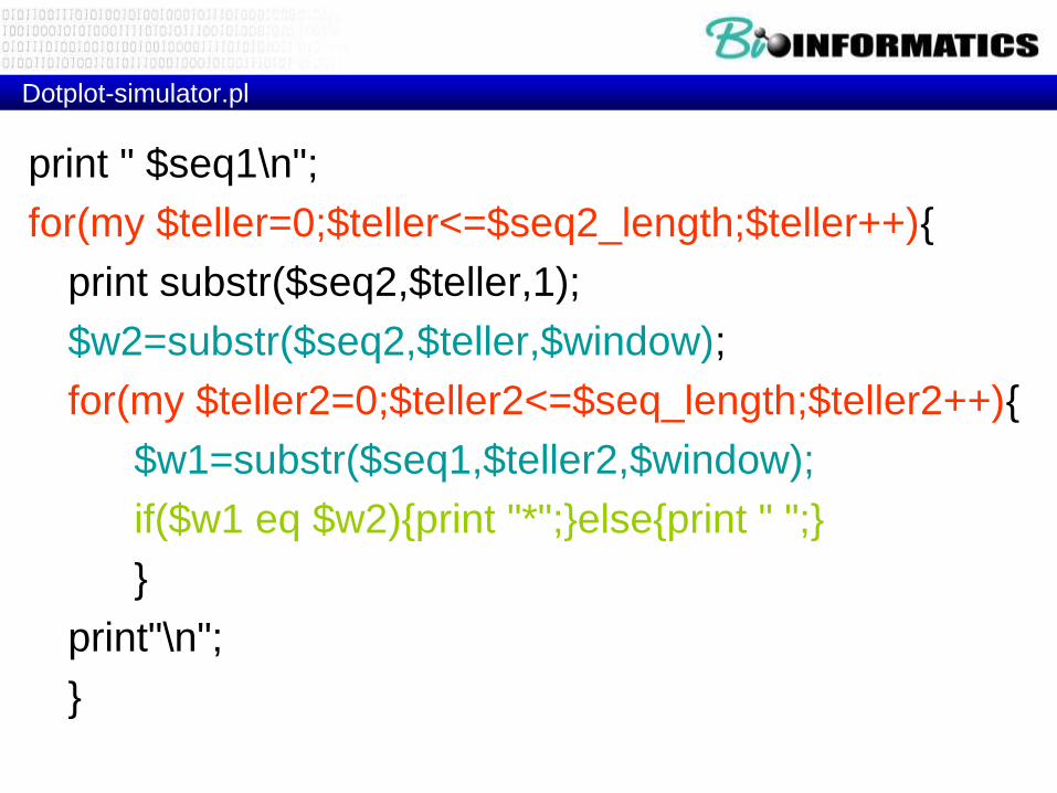
Dotplot-simulator.pl

print " $seq1\n";

for(my $teller=0;$teller<=$seq2_length;$teller++){

print substr($seq2,$teller,1);

$w2=substr($seq2,$teller,$window);

for(my $teller2=0;$teller2<=$seq_length;$teller2++){

$w1=substr($seq1,$teller2,$window);

if($w1 eq $w2){print "*";}else{print " ";}

}

print"\n";

}

Overview

Window size = 1, stringency 100%

Noise in Dot Plots

• Nucleic Acids (DNA, RNA)

– 1 out of 4 bases matches at random

• Stringency

– Window size is considered

– Percentage of bases matching in the window is

set as threshold

Reduction of Dot Plot Noise

Self alignment of ACCTGAGCTCACCTGAGTTA

Dotplot-simulator.pl

Example: ZK822 Genomic and cDNA

Gene prediction:

How many exons ?

Confirm donor and aceptor sites ?

Remember to check the reverse complement !

Chromosome Y self comparison

• Regions of similarity appear

as diagonal runs of dots

• Reverse diagonals

(perpendicular to diagonal)

indicate inversions

• Reverse diagonals crossing

diagonals (Xs) indicate

palindromes

• A gap is introduced by each

vertical or horizontal skip

Overview

• Window size changes with goal

of analysis

– size of average exon

– size of average protein structural

element

– size of gene promoter

– size of enzyme active site

Overview

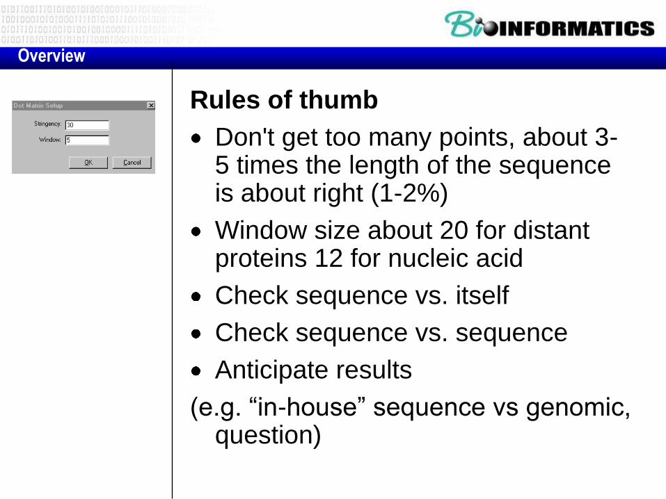
Rules of thumb

Don't get too many points, about 3-5 times the length of the sequence is about right (1-2%)

Window size about 20 for distant proteins 12 for nucleic acid

Check sequence vs. itself

Check sequence vs. sequence

Anticipate results

(e.g. “in-house” sequence vs genomic, question)

Overview

Available Dot Plot Programs

Dotlet (Java Applet)

http://www.isrec.isb-

sib.ch/java/dotlet/Dotlet.

html

http://www.isrec.isb-sib.ch/java/dotlet/Dotlet.html





Dotter (http://www.cgr.ki.se/cgr/groups/sonnhammer/Dotter.html)


EMBOSS DotMatcher, DotPath,DotUp

http://bioinfo.pbi.nrc.ca:8090/EMBOSS/runs/filejKtqWM/dotmatcher.1.png

http://bioinfo.pbi.nrc.ca:8090/EMBOSS/runs/fileZr0f9M/dottup.1.png

Weblems

• W3.1: Why does 2 PAM, i.e. 1 PAM multiplied with itself, not correspond to exactly 2% of the amino acids having mutated, but a little less than 2% ? Or, in other words, why does a 250 PAM matrix not correspond to 250% accepted mutations ?

• W3.2: Is it biologically plausible that the C-C and W-W entries in the scoring matrices are the most prominent ? Which entries (or groups of entries) are the least prominent ?

• W3.3: What is OMIM ? How many entries are there ? What percentage of OMIM listed diseases has no known (gene) cause ?

• W3.4: Pick one disease mapped to chromosome Y from OMIM where only a mapping region is known. How many candidate genes can you find in the locus using ENSEMBL ? Can you link ontology terms for the candidates to the disease phenotype ?

bioinformatica t3-scoring matrices

Education

aminoacid properties

polar amino acid groups

identical amino acids

occuring amino acids

observed amino acid

identity matrix

scoring matrix

genetic code changes