basic quantum circuits for classification and

Int. J. Appl. Math. Comput. Sci., 2020, Vol. 30, No. 4, 733–744DOI: 10.34768/amcs-2020-0054

BASIC QUANTUM CIRCUITS FOR CLASSIFICATIONAND APPROXIMATION TASKS

JOANNA WISNIEWSKA a,∗, MAREK SAWERWAIN b, ANDRZEJ OBUCHOWICZ b

aInstitute of Information SystemsMilitary University of Technology

ul. Gen. S. Kaliskiego 2, 00-908 Warsaw, Polande-mail: [email protected]

bInstitute of Control and Computation EngineeringUniversity of Zielona Góra

ul. Szafrana 2, 65-516 Zielona Góra, Polande-mail: M.Sawerwain,[email protected]

We discuss a quantum circuit construction designed for classification. The circuit is built of regularly placed elementaryquantum gates, which implies the simplicity of the presented solution. The realization of the classification task is possibleafter the procedure of supervised learning which constitutes parameter optimization of Pauli gates. The process of learningcan be performed by a physical quantum machine but also by simulation of quantum computation on a classical computer.The parameters of Pauli gates are selected by calculating changes in the gradient for different sets of these parameters. Theproposed solution was successfully tested in binary classification and estimation of basic non-linear function values, e.g.,the sine, the cosine, and the tangent. In both the cases, the circuit construction uses one or more identical unitary operations,and contains only two qubits and three quantum gates. This simplicity is a great advantage because it enables the practicalimplementation on quantum machines easily accessible in the nearest future.

Keywords: quantum circuits, data classification, supervised learning, qubits, qudits.

1. Introduction

Machine learning as a field of the computer science is verypopular. The idea of artificial intelligence is exhilaratingsince the 1940s when the first model of an artificial neuron(the so-called McCulloch–Pitts neuron) was presented.Artificial neural networks and other tools of machinelearning still evolve, and play a more and more importantrole in data processing. Today, the whole world is on theverge of a quantum revolution where data are going to beencoded as quantum states and processed with the use oflaws of quantum mechanics (Nielsen and Chuang, 2010;Kołaczek et al., 2019) and machine learning methodsare also developed for quantum computational systems.Researchers deal with the different kinds of quantummachine learning (Biamonte et al., 2017; Schuld et al.,2014; 2015), e.g., quantum neural networks (Narayananand Menneer, 2000; Zoufal et al., 2019), quantum kNN

∗Corresponding author

methods (Wiebe et al., 2015), quantum self-organizedmaps (Weigang, 1998), or the quantum k-means method(Veenman and Reinders, 2005).

In this work, we would like to propose a newsolution from the group of quantum machine learningmethods: a classifying quantum circuit (the article isan extended version of an earlier conference paper byWisniewska and Sawerwain (2020)). The circuit differsfrom the existing approaches because input data are ina form of quantum states (classical observations as inputdata were suggested by Pérez-Salinas et al. (2020)), andonly two kinds of quantum gates are used (much morecomplicated circuits were proposed by Mitarai et al.(2018)). These gates realize operations of rotations andintroduce entanglement. The angles of rotations arecalculated with optimization methods (Li et al., 2017).

The article is organized as follows. In Section 2 basicdefinitions referring to quantum computing are presented.They cover a fundamental part of quantum mechanics

mailto:[email protected]

mailto:M.Sawerwain,[email protected]

734 J. Wisniewska et al.

needed to present the content connected with the quantumapproach to machine learning. A broad introduction toquantum computing can be found in the monograph byMacMahon (2007).

Section 3 contains information concerningthe conversion of classical data to quantum states,construction of the circuit, and the learning algorithm. InSection 4, we present results of numerical experimentsfor classification tasks realized as simulation of quantumcomputation. Section 5 includes a summary andconclusions.

2. Brief introduction to quantuminformation processing

We utilize standard denotation, e.g., N for naturalnumbers. For convenience and clarity, all the symbolsused are gathered in Table 1.

An equivalent of the classical bit in quantumcomputing is the so-called qubit. According to the lawsof quantum mechanics, a description of a qubit is adescription of a quantum state. While quantum states maybe expressed as elements of a Hilbert space, i.e., vectorswhose entries are complex numbers C, a single qubit’sstate may be presented as a vector

|ψ〉 =[α0

α1

], (1)

under the normalization condition |α0|2 + |α1|2 = 1,where α0, α1 ∈ C, and |ψ〉 denotes a column vector inthe so-called Dirac notation.

A qubit may be broaden to a qudit, i.e., to a generalquantum information unit. Let d stand for the freedomlevel of a qudit. The state of a single qudit is a normalizedd-element vector of complex numbers.

In classical computing, the bits are usually denotedas one or zero. Of course, two arbitrary separate states aresufficient to realize a calculation with the use of Booleanalgebra. Naturally, the logic invented by George Boolecan be extended to multivalued logic (Augusto, 2017). Asimilar approach is utilized in quantum computing, wherewe employ the so-called computational basis. A basisfor a d-level qudit contains d orthonormal d-dimensionalvectors. A basis which is the most used in the area ofquantum computational methods is termed the standardbasis. The vectors of this basis are constructed in thefollowing way: d− 1 elements are zeros and one elementequals one (this element occupies a different position ineach basis vector). For example, if we deal with qutrits(qudits with d = 3), then

|0〉 =⎡⎣ 1

00

⎤⎦ , |1〉 =

⎡⎣ 0

10

⎤⎦ , |2〉 =

⎡⎣ 0

01

⎤⎦ . (2)

Table 1. Symbols and notation used in the paper.

Notation Description

N, R, C integer, real, and complex numbersU the set of unitary operators

〈M〉the expectation of operator Mon quantum state |ψ〉: 〈M〉 =〈ψ|M |ψ〉

i, j,m, k, l, r

indexes, i.e., integer values usedto enumerate operators, probes,attributes; always used locally inthe context of a given notion orequation

G, Γk

the generalized set of Paulioperators of dimensionality d(including traditional X,Y, Zoperators for d = 2), together withan identity operator, is denoted byG, and Γk refers the k-th operatorconstructed from the SU(d) groupwhich is more general than thegeneralized set of Pauli operators

RΓk

rotation operator, where Γkrepresents one of the generalizedPauli operators

Θk,j , βk,j , ηr,r examples of SU(d) operatorsξld the l-th root of unity of degree d

CNOT the controlled negation gate

Uione of unitary operators used tobuild the classification circuit

ζ the total number of U operators

θ, θiall θ parameters and one or set ofparameters for a given operator Ui

Hc, Dcthe height and depth (number oflayers) of the classifying circuit

|ψ〉 quantum state of one qubit or qudit

|ψd〉, |ψc〉a general description of qubits orqudits containing: data sample(also called an observation), classlabel

|ψxi

d 〉, |ψxic 〉

quantum states which describe agiven data sample xi (|ψxi

d 〉), anda class label related to sample xi(|ψxi

c 〉)X a data setxi the i-th value of from the data setL loss function

dthe number of attributes for a givenobservation, and also the freedomlevel of a qudit

All basis vectors satisfy the normalization condition, andare orthogonal one to another.

Aparat from the normalized vectors, the principleof superposition is often utilized to express the quantum

Basic quantum circuits for classification and approximation tasks 735

state. This notion describes the state in relation to thechosen computational basis. For example, the state of ad-level qudit in the standard basis is

|ψ〉 = α0|0〉+ α1|1〉+ · · ·+ αd−1|d− 1〉, (3)

where∑d−1i=0 |αi|2 = 1, and αi ∈ C. Coefficients αi are

called the probability amplitudes or just the amplitudes.A single qubit or a qudit are not very useful for

any calculation. Let n be the number of units in theso-called quantum register. The state of a register maybe expressed as a tensor product of vectors describingconsecutive qudits. Of course, the same rule concerns thestates written as a superposition. The state of two qubitsis

|Ψ〉 = |ψ〉 ⊗ |φ〉= (α0|0〉+ α1|1〉)⊗ (β0|0〉+ β1|1〉)= α0β0|00〉+ α0β1|01〉+ α1β0|10〉+ α1β1|11〉,

(4)

where products αiβj are amplitudes of the state andsatisfy the normalization condition.

Remark 1. (Quantum entangled states) It should beemphasized that some quantum states cannot be presenteddirectly as a tensor products of other states. Such statesare called entangled states.

Apart from vectors and superposition, quantum statesmay be denoted as density matrices. The discussion in thiswork is based on pure states where the density matrix ρ iscalculated as the outer product of state vectors,

ρ = |Ψ〉〈Ψ|, (5)

where 〈Ψ| is the Hermitian adjoint of |Ψ〉 whichrepresents an arbitrary pure quantum state (also termedthe vector state). The quantum states described bydensity matrices are used in the description of the learningalgorithm in Section 3.3.

If we want to perform computation on an inputquantum state, we have to transform it. This operationmay have a unitary or a non-unitary character. The unitarytransformations are reversible. We can denote the actionperformed on a quantum state |ψin〉 (in order to obtain|ψout〉) with the use of a unitary operator U as

U |ψin〉 = |ψout〉, (6)

and the operator is unitary if U † = U−1 (where † standsfor the Hermitian adjoint operation, and −1 signifies theinversion operation). Operator U may be expressed as amatrix. If we deal with an n-qudit state, the size of thematrix is dn × dn (so the vector |ψout〉 may be computedby the multiplication of matrix U by the vector |ψin〉).

Quantum gates are unitary operators. In this work,we utilize the negation gate, the gate realizing qubit’s

rotation through π radians around the z-axis, and theHadamard gate for qubits, and their generalizations forqudits.

The state of a single qubit can be visualized on thethree-dimensional (x, y, z) Bloch sphere where the anglebetween orthonormal vectors is π. The Pauli operatorsrealize basic π-radian rotations around the x-axis, y-axisand z-axis, respectively,

X =

[0 11 0

],

Y =

[0 −

0

],

Z =

[1 00 −1

].

(7)

Let us denote by Γ = I,X, Y, Z the set of Paulioperators together with the identity operator I (identitymatrix).

The gate X is termed the negation gate. Ina two-qubit system, we can introduce the controllednegation gate:

CNOT =

⎡⎢⎢⎣

1 0 0 00 1 0 00 0 0 10 0 1 0

⎤⎥⎥⎦ . (8)

The qubit gates can be also directly generalized totheir qudit versions. Denote by |l〉 one of d vectors fromthe standard basis. The single qudit negation gate Xperforms the operation

X |l〉 = |(l + 1) mod d〉. (9)

The rotation gate Z changes the qudit’s phase:

Z|l〉 = exp((2πl)/d)|l〉 = ξld|k〉, (10)

where ξld = exp((2πl)/d) are the roots of unity.The operators X and Z are elements of the so-calledgeneralized Pauli group where they are denoted as Gj,l

(an additional index j = 0, . . . , d− 1):

Gj,l = ZjX l = ξjld XlZj, (11)

where Xd = Zd = I , and Id×d represents the identityoperator. However, it should be mentioned that thegeneralized operators from the Pauli group can be fullyreconstructed with the SU(d) operators which are givenin the following paragraph.

The construction of the classifying circuit, presentedin this work, needs gates realizing rotations by any angleϑ ∈ R. Therefore, we can introduce a set of gatesRΓk

(ϑ)which realizes rotations by angle ϑ on the planes pointedout by an appropriate set of operators from the SU(d)


group, and this allows us to replace the generalized PauligroupG with the SU(d) operators.

The procedure of constructing SU(d) operators isuniversally defined for qudits, so it generates gates forpointed freedom level d. We begin with defining the set ofprojectors P k,j for each k and j such that 1 ≤ k < j ≤ d,and υ, μ fulfill the relation 1 ≤ υ, μ ≤ d:

P k,j = |k〉〈j| = [pυ,μ]d×d, pυ,μ = δυ,jδμ,k, (12)

where P k,j means that a value of one is in the k-th rowand the j-th column, pυ,μ are entries ofP k,j . The symbolsδυ,j δμ,k are the Kronecker deltas, and the result of theirproduct is placed in the k-th row and j-th column ofmatrix P . The set of d(d − 1) generators, derived fromthe group SU(d), is

Θk,j = P k,j + P j,k, βk,j = −i(P k,j − P j,k) (13)

for each pair of indexes k and j, where Θk,j arecounterparts of the Pauli X operator, and βk,j areequivalents of the Pauli Y operator. Finally, the last setof d− 1 generators is

ηr,r =

√2

r(r + 1)

[( r∑j=1

P j,j)− rP r+1,r+1

], (14)

where 1 ≤ r ≤ (d − 1), and ηr,r correspond to the PauliZ operator.

Other details about the construction of SU(d)operators are given by Bertlmann and Krammer (2008).

The qudit-rotating gates RΓk(ϑ) can be defined with

the use of operators Θk,j , βk,j , and ηr,r as consecutiveΓk (where k = 1, . . . , d2 − 1). Particular rotations can berealized as the operator

RΓk(ϑ) = exp

(Γkϑ

d

), (15)

where ϑ ∈ R. These rotation gates are also unitary, whichis easy to verify throughRΓk

(ϑ)R†Γk(ϑ) = I .

To induce an entanglement in a two-qubit system, weneed only one Hadamard gate and one CNOT gate. TheCNOT for qudits may be defined as

CX|x〉|y〉 = |x〉|(−x − y) mod d〉. (16)

Let us now briefly discuss non-unitary operations.In this work, we utilize a non-reversible operation whichis quantum measurement. In detail, this transformationis the von Neumann projective measurement. Projectivemeasurements always refer to a given computational basisbecause these operations tend to project a whole quantumstate or just some specified qudits to one of basis vectors.

Let us mark the initial one-qudit state as|ψin〉, and a basis as a orthonormal set of vectors

|u0〉, |u1〉, . . . , |ud−1〉. Performing the von Neumannmeasurement, which is used in the discussed classificationcircuit, requires the definition of the observable

M =

d−1∑i=0

λiPi, (17)

where λi are the eigenvalues associated with projectorsPi, and consecutive Pi = |ui〉〈ui|. The values λi arethe measurement results. The probability of receivingparticular λi is p(λi) = 〈ψin|Pi|ψin〉. The state of thequdit after the measurement is described by

|ψout〉 = Pi|ψin〉√〈ψin|Pi|ψin〉=

Pi|ψin〉√p(λi)

. (18)

Because the character of quantum computations isprobabilistic, each experiment must be performed manytimes, and finished with a measurement. The final result ofcomputation is obtained as a probability distribution fromall received outcomes. We use the expected value 〈M〉which describes an average value of measurement resultsperformed by observableM on state |ψ〉:

〈M〉 = 〈ψ|M |ψ〉. (19)

Additionally, to evaluate if the classification wascarried out correctly, we need a measure which estimatesthe similarity of two quantum states. In this work, we referto the fidelity measure (MacMahon, 2007). The fidelitymeasure for pure quantum states is calculates as

F (ρ, δ) = Tr(√√

ρδ√ρ)= |〈φ|ψ〉|, (20)

where ρ and δ are density matrices: ρ = |ψ〉〈ψ|, δ =|φ〉〈φ|, and 0 ≤ F (ρ, δ) ≤ 1. The higher fidelity, themore similar states |ψ〉 and |φ〉.

3. Quantum computations for dataclassification

In this section, we propose a classifying quantum circuitbased on a supervised learning approach. The aim of thissection is to present introductory information concerninga unitary operation responsible for classification. Next,some details about the probability distribution and the lossfunction are given. The preparation of classical data to besuitable for a quantum circuit is described in Section 3.1.

We assume that there is a function f which classifiesN elements of a data set X = xi. A set R = ri,where ri = f(xi), contains information specifying whichclasses particular samples/observations xi belong to.

The above-mentioned quantum circuit may beunderstood as a unitary operator which transforms avector quantum state during the classification. This


operation and its equivalent notation (with the use of adensity matrix) may be presented as

|ψc〉 = U(θ)|ψd〉, ρc = U(θ)ρdU†(θ), (21)

where ρc = |ψc〉〈ψc| and ρd = |ψd〉〈ψd|.The state |ψd〉 (or ρd) serves to encode the sample

of classical information xi. Marking |ψxi

d 〉 describes thecorrect quantum state which refers to the observation xi(the procedure of converting classical data to quantumstates is presented in Section 3.1). Here |ψc〉 includes theinformation regarding the class, and especially the state|ψxic 〉 contains a label for the observation xi. The unitary

operation U , depending on the parameter set θ, acts as aclassification function f .

Remark 2. (Probability distribution of the final state mea-surement) It should be emphasized that after the operationU a measurement of the resulting quantum state mustbe performed. Estimation of the probability distributionfor |ψc〉 requires many repetitions of the whole process.Precisely, to reach accuracy ε, an experiment has to beperformedO(N/ε2) times.

If the classifying circuit generates a state |ψc〉, whichassigns an observation to a class correctly, then it ispossible to introduce the distance between the value f(xi)and the expectation for the sample xi:

dist =∣∣∣∣∣∣f(xi)− Λ

(〈M〉xi

ψc

)∣∣∣∣∣∣ , (22)

where 〈M〉xi

ψcis the expected value connected to the

measurement of the final state |ψc〉, xi being anobservation from the data setX . HereΛ may be used as anelement of additional classical processing (see Remark 3).

Small values of dist specify correct classification.For a given set of observations, we seek a form of U(θ)minimizing the value of the loss function

L =∑i

∣∣∣∣∣∣f(xi)− Λ

(〈M〉xi

ψc

)∣∣∣∣∣∣2, (23)

where parameters θ are decision variables in theoptimization problem, and Λ again is an additionalfunction which can be used to connect the obtainedexpected value with the class label of the sample xi.

Remark 3. (Role of the Λ function) It should beemphasized that the values of f(xi) and 〈M〉xi

ψcare real

numbers. The role of the function Λ is supplementaryconversion of expectation to a real number representinga class label of a sample xi, i.e., it can rescale theexpectation to another range compatible with the valuesof the f(·) function. However, in our case, we do not usethe function Λ in our experiments, because the probabilityvalues after the measurement of state 〈M〉xi

ψcare sufficient

to make a correct classification (otherwise, the use of afunction Λ should be considered).

3.1. Converting classical data to quantum states.Quantum computation needs specific data preparation.The observations have to be correct quantum states. InSection 4, we present the results of classification but,beforehand, it is meaningful to show the methods ofclassical data conversion to quantum states for examplesdescribed in Section 4.

The first step in the conversion is a procedure ofdata normalization (Li and Li, 2015), used in classicalmachine learning and data mining. Assume that a learningset X containsN observations with d attributes/variables.The normalization needs calculating the range of acceptedvalues for each i-th attribute (i = 0, . . . , (d − 1)),so extreme values have to be determined, maxiX andminiX . If xi,m stands for the i-th attribute in the m-thobservation (m = 1, . . . , N ), the normalized value is

xi,m =xi,m −miniX

maxiX −miniX. (24)

Remark 4. After normalization, we have xi,m ∈[0, 1]. In classical machine learning and data mining, thissolution avoids exaggerated influence of some variables(e.g., with different magnitude values than other variables)on the model. The normalization is also helpful during theprocess of converting classical data to quantum states.

At this point, each attribute value within oneobservation is less than one, but the sum of their squaredmoduli, probably, does not equal one. Now, we have tocarry out the second part of the conversion to meet thequantum normalization condition.

We would like to encode one d-attribute observationas a state of one d-level qudit. This qudit’s i-th amplitudevalue is calculated as

αmi =

√xi,m∑d−1l=0 xl,m

, (25)

where m is the number of the observation. We processall attributes this way, in each observation, and obtainan N -element set of quantum states needed for theexperiments with the classifying quantum circuit.

After normalization, we obtain quantum states whichcan be transformed by a quantum circuit. However, thesedata may be utilized, e.g., as a basis for the constructionof a two-label quantum state:

|ψ〉 = sin(a0 + b0αm0 )|0〉+ cos(a1 + b1α

m1 )|1〉, (26)

where a0 and b0 represent the additional constantsencoding data for the class label zero, and respectively,a1, b1 for the class label one. These parameters help us toimprove the quality of classification. In the case of qudits


(where dimensions are denoted by d), the quantum statecan be expressed with the use of RΓk

(ϑ) rotation gates:

|ψ〉 =d−1∏i=0

RΓk(ai + biα

mi )|i〉, (27)

where the Γk’s describe the gates based on the operatorΘk,j , and constants ai, bi play the same role as in theprevious case for qubits.

Remark 5. (Value selection for ai and bi) It should beemphasized that constants ai and bi are directly set duringlearning. In the presented examples, we assume that ai =0 and bi = 1. Selection of these values in the processof data preparation introduces preliminary demarcation ofsamples.

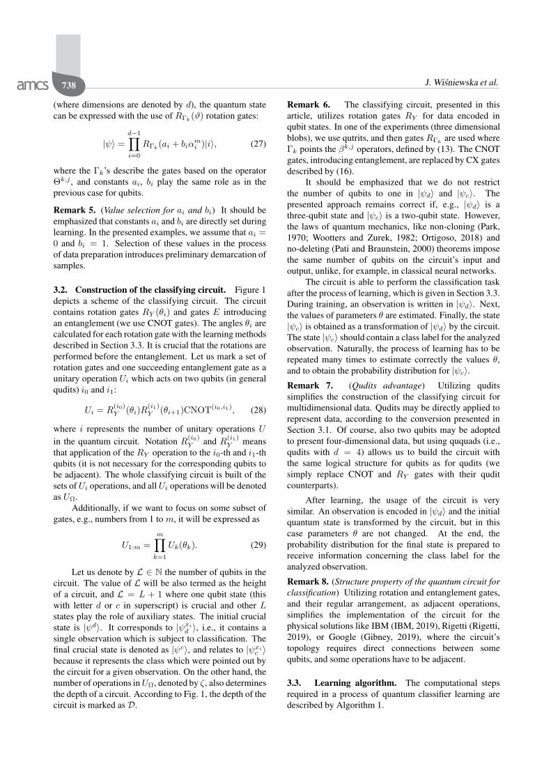
3.2. Construction of the classifying circuit. Figure 1depicts a scheme of the classifying circuit. The circuitcontains rotation gates RY (θi) and gates E introducingan entanglement (we use CNOT gates). The angles θi arecalculated for each rotation gate with the learning methodsdescribed in Section 3.3. It is crucial that the rotations areperformed before the entanglement. Let us mark a set ofrotation gates and one succeeding entanglement gate as aunitary operation Ui which acts on two qubits (in generalqudits) i0 and i1:

Ui = R(i0)Y (θi)R

(i1)Y (θi+1)CNOT(i0,i1), (28)

where i represents the number of unitary operations Uin the quantum circuit. Notation R(i0)

Y and R(i1)Y means

that application of the RY operation to the i0-th and i1-thqubits (it is not necessary for the corresponding qubits tobe adjacent). The whole classifying circuit is built of thesets ofUi operations, and allUi operations will be denotedas UΩ.

Additionally, if we want to focus on some subset ofgates, e.g., numbers from 1 to m, it will be expressed as

U1:m =

m∏k=1

Uk(θk). (29)

Let us denote by L ∈ N the number of qubits in thecircuit. The value of L will be also termed as the heightof a circuit, and L = L + 1 where one qubit state (thiswith letter d or c in superscript) is crucial and other Lstates play the role of auxiliary states. The initial crucialstate is |ψd〉. It corresponds to |ψxi

d 〉, i.e., it contains asingle observation which is subject to classification. Thefinal crucial state is denoted as |ψc〉, and relates to |ψxi

c 〉because it represents the class which were pointed out bythe circuit for a given observation. On the other hand, thenumber of operations inUΩ, denoted by ζ, also determinesthe depth of a circuit. According to Fig. 1, the depth of thecircuit is marked as D.

Remark 6. The classifying circuit, presented in thisarticle, utilizes rotation gates RY for data encoded inqubit states. In one of the experiments (three dimensionalblobs), we use qutrits, and then gates RΓk

are used whereΓk points the βk,j operators, defined by (13). The CNOTgates, introducing entanglement, are replaced by CX gatesdescribed by (16).

It should be emphasized that we do not restrictthe number of qubits to one in |ψd〉 and |ψc〉. Thepresented approach remains correct if, e.g., |ψd〉 is athree-qubit state and |ψc〉 is a two-qubit state. However,the laws of quantum mechanics, like non-cloning (Park,1970; Wootters and Zurek, 1982; Ortigoso, 2018) andno-deleting (Pati and Braunstein, 2000) theorems imposethe same number of qubits on the circuit’s input andoutput, unlike, for example, in classical neural networks.

The circuit is able to perform the classification taskafter the process of learning, which is given in Section 3.3.During training, an observation is written in |ψd〉. Next,the values of parameters θ are estimated. Finally, the state|ψc〉 is obtained as a transformation of |ψd〉 by the circuit.The state |ψc〉 should contain a class label for the analyzedobservation. Naturally, the process of learning has to berepeated many times to estimate correctly the values θ,and to obtain the probability distribution for |ψc〉.Remark 7. (Qudits advantage) Utilizing quditssimplifies the construction of the classifying circuit formultidimensional data. Qudits may be directly applied torepresent data, according to the conversion presented inSection 3.1. Of course, also two qubits may be adoptedto present four-dimensional data, but using ququads (i.e.,qudits with d = 4) allows us to build the circuit withthe same logical structure for qubits as for qudits (wesimply replace CNOT and RY gates with their quditcounterparts).

After learning, the usage of the circuit is verysimilar. An observation is encoded in |ψd〉 and the initialquantum state is transformed by the circuit, but in thiscase parameters θ are not changed. At the end, theprobability distribution for the final state is prepared toreceive information concerning the class label for theanalyzed observation.

Remark 8. (Structure property of the quantum circuit forclassification) Utilizing rotation and entanglement gates,and their regular arrangement, as adjacent operations,simplifies the implementation of the circuit for thephysical solutions like IBM (IBM, 2019), Rigetti (Rigetti,2019), or Google (Gibney, 2019), where the circuit’stopology requires direct connections between somequbits, and some operations have to be adjacent.

3.3. Learning algorithm. The computational stepsrequired in a process of quantum classifier learning aredescribed by Algorithm 1.


|ψd〉

|ψc〉

|0〉

|ψ3〉

|ψ4〉

|ψ1〉

|ψ2〉

|0〉

|0〉

|0〉

Circuit with particular gates (B)

|0〉

|ψL〉

RY (θi)

RY (θi) E RY (θi)

RY (θi)

RY (θi) E RY (θi) E RY (θi)

RY (θi)

RY (θi) E ERY (θi)

U1

U2

Um

Um+1

Uζ

|ψd〉|0〉|0〉|0〉

|0〉|0〉

|0〉|0〉|0〉|0〉

U1

U2

U3

U4

Um−1

Um+1

|0〉|0〉

Um

Um+2

Um+t1

Uζ

|ψ3〉|ψ4〉

|ψ1〉|ψ2〉

|ψ7〉|ψ8〉

|ψ5〉|ψ6〉

|ψc〉|ψL〉|ψL−1〉|ψL−2〉h

eightofthecircuit

Hc

General scheme of the circuit (A)

(C)

RY

RY

(D)

RY

RY

RY

RY RY

RY

depth of the circuit Dc

Um+t1+t2

Um+t1+1

(E)

RY

RY

RY

RY RY

RY

RY

RY

RY

RY

RY

RY

one layer

Fig. 1. General structure of the quantum circuit for data classification. The quantum circuit (a) depicts how the operation Ui isperformed on particular qubits/qudits. The circuit (b) presents types of gates utilized in the classifying circuit. The controlledgates E introduce the entanglement, and here the CNOT gates are used. Gates RY (θi), with optimized parameters θ, areresponsible for rotations around the y-axis (for qubits, but for qudits rotation planes are pointed out by the operators RΓk(ϑi)).The qubit/qudit |ψd〉 represents the input data, and the qubit/qudit |ψc〉 is the final state pointing out a class of the analyzedsample. The additional qubits/qudits |ψl〉 (where 1 ≤ j ≤ L, and L ∈ N) play the ancillary role and are not significant fordata classification. The circuits (c), (d) and (e) are examples of circuits which may be constructed as special cases of schemes(a) and (b). The circuit (e) was used in the numerical experiments in this work (the parameters θi for RY gates are omitted toincrease readability).

Remark 9. After learning, validation is recommended.The new form of the operator U(θ) should be verified ona test data set to assess if the selection of parameters θ iseffective, i.e., the value of L was diminished.

The most important step in the procedure of learningis calculating the angles θi for each rotation gate, in thecontext of input data. The classifying circuit realizes asequence of unitary operations Ui, and the expectationfor the observable M , utilized in the last measurement,depends on the parameters θi:

〈M(θ)〉 = Tr(MUiρdUi

†)

for all i. (30)

The operations Ui consist of gates R and CNOT, so

the gradient may be calculated as

∂〈M〉∂θi

= −

2Tr

(MUi:ζ

[Γ(i)k , U1:i−1ρdU

†1:i−1

]Ui:ζ

†), (31)

where Γ(i)k denotes that one of the generalized Pauli

operators is applied to the i-th qubit/qudit. Theabove relation contains a commutator which cannot becalculated directly. The operations Ui appear on both thesides of the equation, and values θi are also unknown.However, the rotation angles θ may be computed with theuse of arbitrary ρ (Li et al., 2017), the density matrix ofthe quantum state,


Algorithm 1. Learning algorithm.

(I) Converting classical data xi to the form ofquantum states (see Sec. 3.1).

(II) Performing transformation U with parameters θ on|ψd〉 to obtain a state |ψc〉.

(III) Realizing the measurement procedure and checkingthe class label of the sample (during the learningprocess expectations M are calculated for eachdesirable measurement of significant qubit/qubits inthe state |ψc〉, i.e., f(xi) ≡ 〈MU(θ)|ψxi

d 〉〉xi

ψc.

(IV) Minimizing the loss function L by adjustingparameters θ.

[Γ(l)k , ρ] =

[R

(l)Γk

(π2

)ρR

(l)Γk

(π2

)†

−R(l)Γk

(−π2

)ρR

(l)Γk

(−π2

)†],

(32)

and operatorsR(l)Γk

realize the ±π/2 angle rotation aroundthe X , Y or Z axis with the use of one Pauli operatorΓk on a qubit l (and similarly, in a general case, forqudits where suitable SU(d) operators should be used,however, the correct phase changing needs not onlyintroducing minus or ; for qudits this process requiresd-degree roots of unity). Utilizing this commutatorallows calculating the gradient for angles θ, taking intoconsideration expectationM :

∂〈M〉∂θi

=1

2Tr

(MUi+1:ζUi

(π2

)ρiUi

(π2

)†U †i+1:ζ

)

− 1

2Tr

(MUi+1:ζUi

(−π2

)ρiUi

(−π2

)†U †i+1:ζ

),

(33)

where ρi = U1:iρdU1:i†, and Ui with parameters θi

take previous or initial θi values. Therefore, choosingappropriate versions of rotation gates from the set γ allowscalculating precise values of θi for the expectation 〈M〉±i ,which is also the observable of the |ψc〉 state:

∂〈M〉∂θi

=〈M〉+i − 〈M〉−i

2. (34)

The utilized method is directly derived from the works ofLi et al. (2017) and Mitarai et al. (2018).

4. Numerical experiments

4.1. Data classification. The correctness ofclassification, described in this article, is presented withthe use of Moons, Circles and Blobs data sets (Pedregosaet al., 2011), which contain pairs observation–class label.In this work, data from the first two sets were encoded inqubit states. The Blobs set gives as a prospect to generatetwo and three dimensional observations. We perform twoseparable experiments for this set. In the first one datasamples have two attributes and are encoded as qubits.In the second experiment we utilize samples with threeattributes which are encoded as qutrits, i.e., qudits withd = 3.

In each experiment, 768 samples were used, where512 played the role of a learning set, and the other 256were included in the test (validation) set. The classifyingcircuit utilized two qubits or qutrits, and contained fourlayers of gates. The general scheme of the circuit ispresented in Fig. 1(e).

Figure 2 shows the data sets for binary classification.These sets were subjected to experiments with circuits ofFigs. 1(c) and (d) (see Fig. 1). Figures 2(a)–(g) presentdata after the normalization process, while Figs. 2(d)–(f)depict the same data but as the probability amplitudes ofquantum states before the process of learning. Finally,Figs. 2(g)–(i) show results of the classification (after thelearning process).

It can be seen that after learning the circuit wasable to separate quantum states into two different classes.In the presented cases, the gaps between classes differs.The sizes of the gap are described by parameters ar andbr, given in (26) and (27), and are obtained during thelearning process.

It must be emphasized that Figs. 2(d)–(f) display therepresentation of quantum states from the learning setbefore the learning process. These states are the inputof the circuit and represent data after the normalization,and encoding as the state given in (26), with ai = 0and bi = 1. After learning, the quantum state may becalculated using the partial trace, to inspect the changesbefore the final measurement. In each case, the states areseparated into two classes. Additionally, we can see thatthe states for the Blobs set are properly separated evenbefore the classification process—this is why only one Uioperation is sufficient to realize the classification task.

Table 2 shows the values of fidelity for the test sets.As we can see, the obtained intervals clearly define if thesample belongs to the set labeled as zero or to the setlabeled as one. The samples with the fidelity measuregreater than 0.75 are labeled as zero. The samplesincluded in the first class reach maximally the value offidelity 0.64. This difference in fidelity can be directlydepicted with the previously presented examples fromFig. 2.


0.0 0.2 0.4 0.6 0.8 1.0

x

0.0

0.2

0.4

0.6

0.8

1.0

y

0

1

0.0 0.2 0.4 0.6 0.8 1.0

x

0.0

0.2

0.4

0.6

0.8

1.0

y

0

1

0.0 0.2 0.4 0.6 0.8 1.0

x

0.0

0.2

0.4

0.6

0.8

1.0

y

0

1

(a) (b) (c)

0.2 0.3 0.4 0.5 0.6 0.7

0.70

0.75

0.80

0.85

0.90

0.95

1.00

0.2 0.3 0.4 0.5 0.6 0.7

0.65

0.70

0.75

0.80

0.85

0.90

0.95

1.00

0.0 0.2 0.4 0.6 0.8 1.0

0.0

0.2

0.4

0.6

0.8

1.0

(d) (e) (f)

0.2 0.4 0.6 0.8 1.0

−0.2

0.0

0.2

0.4

0.6

0.8

1.0

0.2 0.4 0.6 0.8 1.0

−0.2

0.0

0.2

0.4

0.6

0.8

1.0

0.0 0.2 0.4 0.6 0.8 1.0

0.0

0.2

0.4

0.6

0.8

1.0

(g) (h) (i)

Fig. 2. Classification of two-dimensional data from the sets Moons, Circle and Blobs. Panels (a)–(c) represent original classical data,(d)–(f) depict data after the normalization, and (g)–(i) show the probability amplitudes of |ψc〉 after learning, but before ameasurement operation on this state.

Table 2. Results of the classification for the sets Moons, Circles,Blobs (for qubits and qutrits) as the intervals of ob-tained Fidelity measure values. The symbol F0 refersto the class labeled as zero, and F1 to that labeled asone.

Set F0 F1

Moons (0.80, 0.95) (0.11, 0.60)Circles (0.75, 0.91) (0.03, 0.46)Blobs (0.83, 0.92) (0.16, 0.64)

Blobs qutrits (0.80, 0.93) (0.15, 0.59)

Figure 3 shows the data classification for the Blobsset with three attributes. In this case, we use qutrits insteadof qubits, but the general structure of the circuit remainsthe same. The gates RY and CNOT are replaced bytheir qutrit equivalents. There is no need to perform anyother additional operations connected with data encoding,

except the steps presented in Section 3.1. If we wouldlike to utilize qubits for this set, then the data should beextra pre-processed or the initial state |ψd〉 should be atwo-qubit state.

4.2. Function approximation. The presentedclassification circuits can be also used as universalapproximators. It means that they are able to estimatevalues of non-linear functions like the sine, the cosine,the hyperbolic tangent or, e.g., exp(−x2).

The approximation of non-linear functions can berealized by the same circuit which was used for theclassification for sets Moons, Circles and Blobs. In thelearning set, we can place input-output pairs (x0, x1)where x0 contains the values of function domain (x0 =〈−1, 1〉), and x1 is the value of the analyzed function.Now, the initial and final states are

|ψd〉 = sin(x0)|0〉+ cos(x0)|1〉,|ψc〉 = sin(x1)|0〉+ cos(x1)|1〉.


0.0 0.2 0.4 0.6 0.8 1.0

x

0.0

0.2

0.4

0.6

0.8

1.0

y

0

1

0.0 0.2 0.4 0.6 0.8 1.0

x

0.0

0.2

0.4

0.6

0.8

1.0

y

0

1

(a) (b)

0.0 0.2 0.4 0.6 0.8 1.0

x

0.0

0.2

0.4

0.6

0.8

1.0

y

0

1

X

0.00.10.20.30.40.50.60.7Y

0.0 0.2 0.4 0.60.8

Z

0.0

0.2

0.4

0.6

0.8

(c) (d)

Fig. 3. Binary classification for the three-attribute data from the Blobs set. Panels (a)–(c) show the data after the normalization processas projections on planes XY , XZ and Y Z. Panels (d) presents the final states |ψc〉 of the qutrit, where particular amplitudesare used as coordinates in a 3D space: two classes of objects are noticeable.

In the learning process, we do not change theloss function but a criterion for the evaluation of theapproximation quality must be added. The quality ofapproximation for the function f can be expressed as ffor the sample xi:

f(xi) = 〈ψxi

d |V |ψxi

d 〉, (35)

where V is a diagonal operator, subjected to optimizationfor the data samples from the set X . The quality rate, inthis case, is

Q =

n∑i=1

(f(x(i))− f(x(i))

)2

, (36)

which is the mean-square error calculated as theaggregated squared difference between the value ofnon-linear function f and the value f approximated bythe quantum circuit.

5. Conclusions

In this article, we have demonstrated that the results of theprevious work of Mitarai et al. (2018), can be applied in aform of much simpler quantum circuits which are able tosolve a classification task. Additionally, the constructionof the corresponding circuits is regular, simple, and easy

to scale for tasks with more variables. Another advantageis that the circuits presented in this paper are also universalapproximators of non-linear functions.

The approach presented in this work is characterizedby the methods of parameters selection, and data read-in,i.e., properly converted data are an input signal forthe circuit, and the parameters selection is based onadjusting angles θ of rotating gates. Therefore, the datais transformed by the circuit as the input states, and thecircuit parameters θ after the learning process remainconstant for the given data set, which makes the circuitreusable (without any changes in parameters θ).

The proposed method of selecting parameter valuesθ is based on a gradient change in rotation angles. Itis able to adjust the circuit parameters so efficientlyfor binary classification that the task is solved withoutany errors (after the learning process, the tests wereperformed with another set of samples, so the model’soverfitting is excluded). Naturally, some data sets containsamples with coordinates pointing out their location closeto samples from another class, and in these cases theclassification process is harder to realize. It should beemphasized that the process of learning may be simulatedon a classical computer but also can be performed on aquantum machine. The simplicity of the proposed circuitmakes this solution suitable for quantum hardware in the


−1.00 −0.75 −0.50 −0.25 0.00 0.25 0.50 0.75

−0.8

−0.6

−0.4

−0.2

0.0

0.2

0.4

0.6

0.8

y=sin(x)

Q=0.017

teacher

approx

inital

−1.00 −0.75 −0.50 −0.25 0.00 0.25 0.50 0.75

0.0

0.2

0.4

0.6

0.8

1.0

y=cos(x)

Q=0.015

teacher

approx

inital

(a) (b)

−1.00 −0.75 −0.50 −0.25 0.00 0.25 0.50 0.75

−0.8

−0.6

−0.4

−0.2

0.0

0.2

0.4

0.6

y= tanh(x)

Q=0.011

teacher

approx

inital

−1.00 −0.75 −0.50 −0.25 0.00 0.25 0.50 0.75

0.0

0.2

0.4

0.6

0.8

1.0

y=exp(−x2)

Q=0.017

teacher

approx

inital

(c) (d)

Fig. 4. Classifying circuit as an approximator of non-linear functions. In all cases, a good quality (the value of parameter Q) ofapproximation was reached. The initial line represents the initial values, and approximated values are depicted by the dashedline. The number of analyzed samples is 20.

nearest future.

Acknowledgment

We would like to thank the Q-INFO group at theInstitute of Control and Computation Engineering (ISSI)of the University of Zielona Góra, Poland, for usefuldiscussions. We also wish to thank the anonymousreferees for valuable comments on the preliminary versionof this paper. The numerical results were obtainedusing the hardware and software available at the GPUμ-Lab located at the Institute of Control and ComputationEngineering of the University of Zielona Góra, Poland.

ReferencesAugusto, L.M. (2017). Many-Valued Logics: A Mathemati-

cal and Computational Introduction, College Publications,London.

Bertlmann, R. and Krammer, P. (2008). Bloch vectors for qudits,Journal of Physics A: Mathematical and Theoretical41(23): 235303, DOI: 10.1088/1751-8113/41/23/235303.

Biamonte, J., Wittek, P., Pancotti, N., Rebentrost, P., Wiebe, N.and Lloyd, S. (2017). Quantum machine learning, Nature549(7671): 195–202, DOI: 10.1038/nature23474.

Gibney, E. (2019). Hello quantum world! Googlepublishes landmark quantum supremacy claim, Nature574(7779): 461–462, DOI: 10.1038/d41586-019-03213-z.

IBM (2019). Q Experience, https://quantum-computing.ibm.com/.

Kołaczek, D., Spisak, B.J. and Wołoszyn, M. (2019). Thephase-space approach to time evolution of quantumstates in confined systems: The spectral split-operatormethod, International Journal of Applied Mathemat-ics and Computer Science 29(3): 439–451, DOI:10.2478/amcs-2019-0032.

Li, J., Yang, X., Peng, X. and Sun, C. (2017). Hybridquantum-classical approach to quantum optimal control,Physical Review Letters 118(15): 150503, DOI:10.1103/PhysRevLett.118.150503.

Li, Z. and Li, P. (2015). Clustering algorithm of quantumself-organization network, Open Journal of Applied Sci-ences 05(6): 270–278, DOI: 10.4236/ojapps.2015.56028.

MacMahon, D. (2007). Quantum Computing Explained, JohnWiley, Hoboken, NJ.

Mitarai, K., Negoro, M., Kitagawa, M. and Fujii, K.(2018). Quantum circuit learning, Physical Review Letters98(3): 032309, DOI: 10.1103/PhysRevA.98.032309.

Narayanan, A. and Menneer, T. (2000). Quantum artificialneural network architectures and components, In-formation Sciences 128(3–4): 231–255, DOI:10.1016/S0020-0255(00)00055-4.

Nielsen, M. and Chuang, I. (2010). Quantum Computa-tion and Quantum Information, 10th Anniversary Edition,Cambridge University Press, Cambridge.

https://quantum-computing.ibm.com/

https://quantum-computing.ibm.com/


Ortigoso, J. (2018). Twelve years before the quantum no-cloningtheorem, American Journal of Physics 86(3): 201–205,DOI: 10.1119/1.5021356.

Park, J. (1970). The concept of transition in quantummechanics, Foundations of Physics 1(1): 23–33, DOI:10.1007/BF00708652.

Pati, A.K. and Braunstein, S.L. (2000). Impossibility of deletingan unknown quantum state, Nature 404(6774): 164–165,DOI: 10.1038/35004532.

Pedregosa, F., Varoquaux, G., Gramfort, A., Michel, V.,Thirion, B., Grisel, O., Blondel, M., Prettenhofer, P.,Weiss, R., Dubourg, V., Vanderplas, J., Passos, A.,Cournapeau, D., Brucher, M., Perrot, M. and Duchesnay,E. (2011). Scikit-learn: Machine learning in Python, Jour-nal of Machine Learning Research 12: 2825–2830, DOI:10.5555/1953048.2078195.

Pérez-Salinas, A., Cervera-Lierta, A., Gil-Fuster, E.and Latorre, J. (2020). Data re-uploading for auniversal quantum classifier, Quantum 4: 226, DOI:10.22331/q-2020-02-06-226.

Rigetti (2019). Quantum Computing Systems, https://www.rigetti.com/systems.

Schuld, M., Sinayskiy, I. and Petruccione, F. (2014). Quantumcomputing for pattern classification, in D.-N. Phamand S.-B. Park (Eds), PRICAI 2014: Trends in Artifi-cial Intelligence, Springer, Cham, pp. 208–220, DOI:10.1007/978-3-319-13560-1_17.

Schuld, M., Sinayskiy, I. and Petruccione, F. (2015).An introduction to quantum machine learning,Contemporary Physics 56(2): 172–185, DOI:10.1080/00107514.2014.964942.

Veenman, C. and Reinders, M. (2005). The nearest sub-classclassifier: a compromise between the nearest mean andnearest neighbor classifier, IEEE Transactions on Pat-tern Analysis and Machine Intelligence 27(9): 1417–1429,DOI: 10.1109/TPAMI.2005.187.

Weigang, L. (1998). A study of parallel self-organizing map,arXiv: quant-ph/9808025v3.

Wiebe, N., Kapoor, A. and Svore, M. (2015). Quantumalgorithms for nearest-neighbor methods for supervisedand unsupervised learning, Quantum Information andComputation 15(3–4): 316–356.

Wisniewska, J. and Sawerwain, M. (2020). Simple quantumcircuits for data classification, in N.T. Nguyen et al. (Eds),Intelligent Information and Database Systems, Springer,Cham, pp. 392–403, DOI: 0.1007/978-3-030-41964-6_34.

Wootters, W. and Zurek, W. (1982). A single quantumcannot be cloned, Nature 299(5886): 802–803, DOI:10.1038/299802a0.

Zoufal, C., Lucchi, A. and Woerner, S. (2019). Quantumgenerative adversarial networks for learning and loadingrandom distributions, Quantum Information 5(1): 103,DOI: 10.1038/s41534-019-0223-2.

Joanna Wisniewska received her MSc degree incomputer science in 2003 at the Military Univer-sity of Technology in Warsaw, Poland. Then shestarted working as a research assistant in the sameuniversity at the Faculty of Cybernetics. She ob-tained her PhD degree in 2012 in the field ofquantum algorithms. As an assistant professor,she continues her research concerning the prob-lems of pattern recognition, quantum algorithms,quantum communication and computer simula-

tion. One of her most important achievements is being a co-author of amonograph on quantum computing published by Polish Scientific Pub-lishers PWN in 2015.

Marek Sawerwain received his ME and PhDdegrees in 2004 and 2010, respectively, at theFaculty of Electrical Engineering, Computer Sci-ence and Telecommunications of the Universityof Zielona Góra, Poland. His current scientificinterests include quantum communication meth-ods, quantum computation methods, and the the-ory of quantum programming languages. He alsoconducts research in the field of quantum compu-tation modeling and simulation, and focuses on

creating effective algorithms for solutions based on modern multicoreCPU and GPU technology. He is currently associated with the Facultyof Computer, Electrical and Control Engineering, University of ZielonaGóra, as an assistant professor.

Andrzej Obuchowicz obtained his MSc (1987)and PhD (1992) degrees in physics, and his DSc(2004) in automatic control and robotics, all fromthe Wrocław University of Technology. Since2015 he has held a full professorial title. He iscurrently the dean of the Faculty of Computer,Electrical and Control Engineering of the Univer-sity of Zielona Góra, Poland. His research inter-ests include soft computing methods, especiallyneural networks, evolutionary algorithms and

other metaheuristic techniques, and their application to global optimiza-tion problems, adaptation in non-stationary environments, computer-aided medical diagnosis, fault tolerant and fault diagnosis systems, themax-plus algebra approach to discrete event systems as well as quantumcomputing. He is the author or a co-author of 4 books and over 120 otherpublications.

Received: 23 January 2020Revised: 9 April 2020Re-revised: 1 July 2020Accepted: 29 October 2020

https://www.rigetti.com/systems

https://www.rigetti.com/systems

basic quantum circuits for classification and

Documents