base level engineering - usgs
TRANSCRIPT

BaseLevelEngineeringRegion 6 Submittal Guidance
April2019

Preface FEMA Region 6 is funding Base Level Engineering (BLE) in watersheds throughout the Region. The investment
in producing broad flood hazard information through the Base Level Engineering methodology will provide
data in the form of engineering models, floodplain extents and other visualization tools that will assist
communities to better determine their flood risk with Estimated Base Flood Elevations (EBFEs).
This guidance document supports effective preparation of Base Level Engineering analysis, including
compilation of the minimum deliverables and datasets. The intent of this document is to provide information
to all Mapping Partners within the Region that are delivering Base Level Engineering throughout Region 6.
Base Level Engineering data will be released with the use of an interactive mapping platform named the
Estimated Base Flood Elevation Viewer (www.infrm.us/estbfe) where users can interact with datasets, point
and click to estimate Base Flood Elevations and download models, spatial data and reports.
This centralized distribution requires a standardized set of deliverables be produced and made available. The
guidance document provides overview and insight into the required delivery of Base Level Engineering
datasets to allow the data prepared to allow data transfer between Mapping Partners, and delivery of all
required information to support broader data sharing with communities through the Estimated Base Flood
Elevation Viewer. Following the guidance document will promote the timely release and availability of Base
Level Engineering data through the interactive viewer.
This guidance document supports effective and efficient implementation of flood risk analysis and mapping
standards codified in the Federal Insurance and Mitigation Administration Policy FP 204‐07801.
For more information, please visit the Federal Emergency Management Agency (FEMA) Guidelines and
Standards for Flood Risk Analysis and Mapping webpage (http://www.fema.gov/guidelines‐and‐standards‐
flood‐risk‐analysis‐and‐mapping), which explains the policy, related guidance, technical references and other
information about the guidelines and standards process.

Document History
Affected Section or Sub‐Section
Date Description
First Tabular Release February 2016 BLE database tables prepared to support development of geodatabase template.
First Narrative Publication
June 2017 Narrative report prepared and tabular guidance previously prepared was expanded upon for use by all active Mapping Partners preparing Base Level Engineering within Region 6.
Submittal Guidance (Spatial Delivery)
November 2017 Updated existing guidance to include additional information to spatial delivery including 2‐D BLE delivery. Also included minor updates to folder structure requirements for MIP upload, XS backwater data inclusion and addition of BFE layer for 2‐D BLE delivery.
Addition of Appendix A November 2017 Appendix A was added to the document to provide Mapping Partners information for the preparation of 2‐D BLE engineering analysis and spatial datasets.
General Document Update
October 2018 Updated to reflect February 2018 guidance and standards update including CNMS, Flood Risk Products, Hazus and the new MIP structure. Also includes new procedure for loading to the new EBFE viewer.
Submittal Guidance (Modeling)
January 2019 Updated guidance to provide outlines and templates to support 2‐D model delivery.
Tips and Tricks January 2019 Additional guidance based on delivery reviews and troubleshooting.
Update to Database files – Hazus Results
April 2019 Update to Spatial Template (Mitigation Layers) to match updates to National Flood Risk Database/Dataset modifications outlined in Flood Risk Database (FRD) Technical Reference, dated February 2018. Updates include:
Remove FRD_Pol_AR
Replace with S_Pol_AR
Remove S_CenBlk_Ar dataset
Replace with S_FRAC_AR dataset
Remove L_RA_Results table
Renamed XS to XS_1D
Renamed BFE to BFE_2D
Added L_Source_Cit table (REQUIRED) for all BLE submittals
Section – Base Level Engineering Data Delivery – updated detail
Section – S_AOMI_PT updated detail
Section – S_AOMI_AR updated detail
Section – Tips and Tricks updated detail
Table of Contents Preface .............................................................................................................................................................. 2
Document History ............................................................................................................................................. 3
Introduction ...................................................................................................................................................... 6
Base Level Engineering ..................................................................................................................................... 6
Sharing data publically through the Estimated Base Flood Elevation Viewer .................................................. 6
Ground Elevation Data Requirements .............................................................................................................. 7
Setting Up a Base Level Engineering Project in the MIP ................................................................................... 7
Partner Responsibilities .................................................................................................................................... 7
Mapping Partner (PTS or CTP) ...................................................................................................................... 7
Regional Service Center (RSC) ....................................................................................................................... 7
FEMA – Region 6 Staff and Regional Program Management Lead (RPML) .................................................. 8
United States Geological Survey (USGS) – Data and Spatial Studies Team .................................................. 8
Additional Contacts ....................................................................................................................................... 9
BLE Delivery Workflow .................................................................................................................................... 10
Base Level Engineering Assessment ‐ Minimum Deliverables ........................................................................ 11
Base Level Engineering Data Delivery ............................................................................................................. 13
Hydraulic Model Data Delivery ....................................................................................................................... 14
2‐D Model Delivery Packaging .................................................................................................................... 15
Spatial Reference Systems .............................................................................................................................. 17
Null Values ...................................................................................................................................................... 17
Topology Rules ................................................................................................................................................ 18
HUC8_StatusInfo ............................................................................................................................................. 19
HUC10_ModelInfo .......................................................................................................................................... 20
S_Pol_AR ......................................................................................................................................................... 21
S_HUC_AR ....................................................................................................................................................... 22
SUB‐BASINS ..................................................................................................................................................... 23
XS_1D .............................................................................................................................................................. 25
BFE_2D ............................................................................................................................................................ 28
WTR_LN .......................................................................................................................................................... 30
WTR_AR .......................................................................................................................................................... 31
DTL_STUD_LN ................................................................................................................................................. 32
DTL_STUD_AR ................................................................................................................................................. 33
FLD_HAZ_AR ................................................................................................................................................... 35
TENPCT_FP ...................................................................................................................................................... 38
Lightest purple hue shows area where ........................................................................................................... 39
BLE_WSE01PCT ............................................................................................................................................... 40
BLE_WSE0_2PCT ............................................................................................................................................. 41
BLE_DEP01PCT ................................................................................................................................................ 42
BLE_DEP0_2PCT .............................................................................................................................................. 43
S_AOMI_PT ..................................................................................................................................................... 44
S_AOMI_AR ..................................................................................................................................................... 48
S_FRAC_AR ...................................................................................................................................................... 51
L_Source_Cit ................................................................................................................................................... 54
CNMS Database .............................................................................................................................................. 56
1. Add Unmapped Miles into S_Studies_Ln: ............................................................................................ 56
2. BLE Tracking Fields: ............................................................................................................................. 57
3. BEING STUDIED Fields: ........................................................................................................................ 58
4. Run the CNMS QC tool: ....................................................................................................................... 59
HAZUS DATASETS ............................................................................................................................................ 63
PRODUCER TIPS & TRICKS ............................................................................................................................... 64
Hydraulic Model Development ................................................................................................................... 64
Flood Risk Dataset Preparation & Data Checks .......................................................................................... 66

Introduction As described in Title 42 of the Code of Federal Regulations, Chapter III, Section 4101(e), once every 5 years,
FEMA must evaluate whether the information on Flood Insurance Rate Maps (FIRMs) reflects the current
risks in flood prone areas. FEMA makes this determination of flood hazard data validity by examining flood
study attributes and change characteristics, as specified in the Validation Checklist of the Coordinated Needs
Management Strategy (CNMS) Technical Reference. The CNMS Validation Checklist provides a series of
critical and secondary checks to determine the validity of flood hazard areas studied by detailed methods
(e.g., Zone AE, AH or AO).
While the critical and secondary elements in CNMS provide a comprehensive method of evaluating the
validity of Zone AE studies, a cost‐effective approach for evaluating Zone A studies has been needed to
address Zone A study miles in the CNMS inventory that are currently “unknown” or that are approaching
their 5‐year expiration and require revalidation. Assessing and evaluating these miles places increased
demands on the Regions in a resource‐constrained environment.
At the start of this effort, the FEMA Region 6 inventory was comprised of more than 70% of Zone A study
miles and approximately 75% of the Region’s flood hazard inventory was currently unknown or unverified.
Base Level Engineering will produce floodplains and modeling allowing the Region to assess its current
effective flood hazard information on FIRMs through the CNMS assessment process. Furthermore, should
the assessment identify an issue with the flooding currently shown on the FIRMs, Base Level Engineering will
provide the data necessary to update FIRMs through the Regulatory Update process, producing and releasing
a preliminary FIRM in the future.
Base Level Engineering Base Level Engineering is an engineering assessment completed for a county, watershed or river basin.
FEMA’s Base Level Engineering (BLE) analysis prepared digital engineering models to determine the potential
flood extents for streams throughout the Nation. Base Level Engineering data offers local community
officials responsible for floodplain management and permitting an advantage by making the calculated water
surface elevation (WSEL) more readily available and more reflective of current conditions.
Base Level Engineering may be produced utilizing one‐dimensional (1‐D) or two‐dimensional (2‐D)
engineering analysis. A good portion of the United States is made up of well‐defined stream channels that
convey storm water runoff where flood risk is appropriately modeled using a 1‐D modeling approach. The
presence of complex, flat, low‐lying and interconnected drainage areas (like the flat and delta areas within
the Region) may benefit from an initial assessment using a 2‐D modeling approach. FEMA Region 6 works
with its State Partners to identify watershed areas that would benefit from 1‐D, 2‐D or a composite
assessment using both 1‐D and 2‐D engineering modeling methodology.
Sharing data publicly through the Estimated Base Flood Elevation Viewer To provide homeowners, businesses and community officials with the best available information on flood risk
outside of GIS, FEMA Region 6 created the Estimated Base Flood Elevation Viewer
(https://webapps.usgs.gov/infrm/estbfe/). This tool provides the opportunity to identify property‐specific
flood elevations with a 1% annual chance of occurring any calendar year in areas where new flood risk data is
available.
To deliver consistent information across all watersheds and with the assistance of various Mapping Partners,
the Region has developed this guidance document to centralize the delivery of datasets for each Base Level
Engineering assessment effort. A database and XML template are also available for use on FEMA Region 6’s
SharePoint Site (BLE Guidance and Tools).

Ground Elevation Data Requirements Base Level engineering shall only be prepared and produced where 90% or greater high‐resolution ground
elevation data is available for use. Existing topographic data leveraged by FEMA must have documentation
that it meets the vertical accuracy requirements detailed in SID43, reproduced in the table below for
reference:
Setting Up a Base Level Engineering Project in the MIP The Mapping Partner and FEMA Project Monitor shall coordinate with the MIP Champ, Jennifer Knecht
([email protected]) to establish the MIP project set up and determine the units of delivery for
each Base Level Engineering project.
Partner Responsibilities The following partners work collaboratively within the responsibilities outlined below to prepare, review and
deliver Base Level Engineering within the Region:
Mapping Partner (PTS or CTP) The Mapping Partners performs the Base Level Engineering assessment and compiles the required minimum
deliverables. The Mapping Partners shall utilize the guidance document to compile and deliver the BLE
datasets outlined within. Special attention should be taken to assure that the files used for the Estimated
BFE Viewer are compiled and prepared in agreement with the information outlined in the later sections of
this guidance.
Regional Service Center (RSC) The Regional Service Center provides technical support for Mapping Partners preparing BLE datasets and
performs a cursory completeness check of Base Level Engineering submittals. The RSC also compiles and
maintains the CNMS coverage showing where Base Level Engineering is in preparation, to support future
project planning for CTPs and the FEMA Region. The Regional Service Center (RSC):
Compiles CNMS data to identify where BLE is active and available throughout the Region.
Performs a review and completeness check of BLE datasets prepared by all Mapping Partners in the
Region. Provides technical support to Mapping Partners actively preparing Base Level Engineering
watershed project areas
Contact information for RSC staff can be found on the next page.

Name/Role Phone Email
Jack Young Regional Technical Coordinator
210.875.0541 [email protected]
Anna Castillo RSC Support, BLE Review Coordination
214.346.6376 [email protected]
Michael Johnson CNMS Lead
612.376.2354 [email protected]
April Smith Base Level Engineering, SME
512.457.7818 [email protected]
FEMA – Region 6 Staff and Regional Program Management Lead (RPML) FEMA will review all incoming datasets prior to their delivery to the USGS Data and Spatial Studies team.
FEMA will work with Mapping Partners to assure that all guidance has been followed and all datasets comply
with the contract delivery requirements and the Base Level Engineering guidance. FEMA PMs work with Matt
Lepinski and the Regional Program Management Lead to review incoming submittals. Once review is
complete, the data is packaged and delivered to the USGS for external accessibility through the Estimated
Base Flood Elevation Viewer.
Name/Role Phone Email
Matt Lepinski Risk Analysis, Engineer
940.297.0235 [email protected]
Elizabeth Savage Regional Program Management Lead (RPML)
214.918.8523 [email protected]
United States Geological Survey (USGS) – Data and Spatial Studies Team The Estimated Base Flood Elevation Viewer was a collaborative effort brought to life by the Data and Spatial
Studies team of the USGS’ Texas Water Science Center. The Region’s collaboration in the Interagency Flood
Risk Management (InFRM) team has allowed this vision to become a reality. The InFRM team strives to
collaborate nationally, to empower locally.
The USGS provides the interactive website – hosting, programming and data housing, as well as, prepares
several Representational State Transfer (REST) services. These REST services allow FEMA to publish one set of
authoritative data, while allowing external partners and entities to ingest these REST services through the
ESRI environment. The USGS Data and Spatial Compiles Regional REST services for the cadastral and
floodplain information, 10%, 1% and 0.2% floodplains, the 1% Water Surface Elevation Grids and the 1%
Flood Depth Grids and provides data storage for all downloadable content available through the website.
Finally, the USGS also reviews incoming questions received through the site and escalates them to FEMA as
necessary for follow up.
Name/Role Phone Email
Kristine Blickenstaff, P.E. Branch Chief‐North Texas Program USGS POC for Site Coordination
682‐316‐5033 [email protected]
Florence Thompson Data Compilation & Distribution
*USGS should not be contacted by Mapping Partners, all Partner questions should be routed through the FEMA
Regional POCs indicated below.

Additional Contacts The Risk Analysis Branch within FEMA Region 6 has worked collaboratively with its Mapping Partners to build
the Estimated Base Flood Elevation Viewer to share elevational data with local communities and residents.
The Base Level Engineering datasets represent a change in the business practices of the Region, led by FEMA
staff, and supported by the Regional Program Management Lead. Should Mapping Partners have any
additional insight or input, one of the following staff may be contacted.
Name/Role Phone Email
Ron Wanhanen Risk Analysis Branch Chief
940.383.7334 [email protected]
Diane Howe Risk MAP Lead
940.898.5171 [email protected]
Matthew Lepinski FEMA POC, Base Level Engineering
940.297.0235 [email protected]
Derek Duskin GIS Lead
940.383.7368 [email protected]
Elizabeth Savage Regional Program Management Lead
214.918.8523 [email protected]

BLE Delivery Workflow The following workflow should be followed by all mapping partners to submit BLE deliverables for upload to
the Estimated BFE Viewer. In general, the watershed will be loaded to the EBFE Viewer within one month
(approximately 4 weeks, 30 days) of the submittal being approved and delivered to the USGS for site load.
Timeframe Workflow Milestones
Mapping Partner Initiates BLE Study
Project Start + 2 weeks
Mapping Partner emails Matt Lepinski (FEMA) and RPML with HUC8_StatusInfo identified. FEMA/RPML will alert RSC for update/inclusion of BLE project area on Status of Studies (SOS) viewer.
Mapping Partner emails Matt Lepinski (FEMA) and RPML with target delivery date for inclusion in HUC10_ModelInfo.
Mapping Partner coordinates with MIP Champ to establish MIP Project Set Up.
Mapping Partner submits CNMS scoping phase update to RSC for incorporation, cc FEMA POC on submittal.
+1 week RSC will update SOS viewer to include project into viewer, including location, status, target delivery date and stream lines.
(OPTIONAL) Mapping Partner Revises Target Delivery Date
Change Request + 1 week
Mapping Partner emails Matt Lepinski (FEMA) and RPML with updated target delivery date (HUC10_ModelInfo).
Mapping Partner coordinates with MIP Champ to establish MIP Project Set Up.
Mapping Partner Completes BLE Watershed
2 Weeks
Mapping Partner emails Matt Lepinski (FEMA) and RPML with HUC10_ModelInfo data requirements identified.
Mapping Partner submits BLE deliverables to Matt Lepinski (FEMA) and RPML via hard drive or FTP site. Physical Address for Hard Drive Delivery:
BLE Data Delivery ATTN: Matt Lepinski FEMA Region 6, Risk Analysis Branch 800 North Loop 288, Denton, Texas 76209
For faster delivery/turn around, Hard Drives may be sent to: BLE Data Delivery ATTN: Elizabeth Savage 9859 Cedarcrest Drive, Aubrey, Texas 76227 Email for FTP delivery (include):
[email protected]; [email protected]; Please note digital submittals will be downloaded by RPML and provided to FEMA for review. Please also carbon copy the FEMA PM for your project delivery area
FEMA reviews the data submission (spatial, model and report) for agreement with submittal guidance. ‐ When requested by FEMA, the RSC may validate the spatial submission (GDB) is using the
current template and all required files are included. FEMA review will review agreement between spatial datasets (grids/floodplains) and assure that all content required for the viewer is available. FEMA validates the submission prior to submittal to the USGS for data being loaded to the Estimated Base Flood Elevation Viewer (www.infrm.us/estbfe)
Coordination will occur between FEMA and submitting Mapping Partner if revisions are needed.
+1‐2 weeks (if required)
FEMA/RPML will review revised BLE submissions for comment incorporation.
FEMA/RSC Approves Submittal – FEMA certifies & Submits to USGS for Data Load
2 Weeks
Once FEMA provides Mapping Partner submits final BLE deliverables to MIP
FEMA provides email with certification of data delivery to USGS
FEMA PM initiates validation of BLE effort in the MIP
USGS begins data preparation and load of BLE watershed.

BLE Watershed Data Available on EBFE Viewer
1 week
USGS notifies FEMA PM that data is available on EBFE viewer
FEMA PM validates MIP Submittal
RPML notifies Mapping Partner, State that watershed is available on Viewer
USGS adds BLE Watershed to download layer on Estimated BFE Viewer
RSC incorporates delivery date and status in Status of Studies
RSC incorporates BLE watershed availability data into CNMS
Base Level Engineering Assessment ‐ Minimum Deliverables All Mapping Partners preparing Base Level Engineering datasets within FEMA Region 6 watershed areas shall
prepare and deliver the following minimum deliverables:
CNMS Scoping Phase delivery within 30 days of project start to update BLE tracking and BEING
STUDIED fields in CNMS including incorporation of unmapped miles. Updated CNMS database is
submitted to the RSC once completed.
Hydrologic modeling utilizing regression equations to prepare flow volumes for the 10%, 4%, 2%, 1%,
1%+, 1%‐, and 0.2% frequency events.
o Mapping Partners shall review results to assure regression equations are not used outside of
the parameters outlined in the equations (i.e. for drainage areas more than the upper limit
for the drainage area)
o Rain‐on grids may also be prepared/produced, if deemed appropriate.
o If a 2‐D approach is selected, Mapping Partners shall refer to Appendix A for additional
guidance related to developing the hydrologic assessment within a project area.
HEC‐RAS modeling shall be prepared for each of the seven flood frequencies listed above. In
addition, the following manual reviews shall be completed during the HEC‐RAS modeling
preparation.
o If BLE is produced for a county or parish‐wide assessment, model streams and cross‐sections
shall be extended to a point where the assessment will produce a complete flood risk
assessment for the county/parish area.
o All hydraulic cross‐sections shall be reviewed for orientation (assuring left to right)
o Where floodplains expand or contract at a large rate, additional cross‐sections shall be
added to the cross‐section file to better describe the natural stream channel
o At locations where in‐line reservoirs exist, the mapping partner shall include an upstream
and downstream face cross‐section, as well as describe the Top of Structure location
(typically with a cross‐section on top of structure).
o At locations where culverts and bridges cross the floodplain, the mapping partner shall
include an upstream and downstream face cross‐section near the structure. Major
structures can be identified by using a roadway geospatial file.
o A point file (S_AOMI_PT) shall be compiled to indicate the location of dams, culverts,
bridges, and other crossings may benefit from locally available structure information to
refine the analysis in the future.
o Model files shall be compiled by stream name/number and organized into HUC10 folders for
delivery
o If a 2‐D approach is selected, Mapping Partners shall refer to Appendix A for additional
guidance related to developing the hydraulic modeling within a project area.

CNMS Production Phase Update for validation assessment shall be completed using the Base Level
Engineering results for all streams existing in the current flood hazard inventory. The updated CNMS
database and supplemental information should be submitted to the Regional Service Center (email
[email protected]) once completed. Provide link to location of data within the Mapping
Information Platform for inclusion in the Regional roll up, performed quarterly.
The Mapping Partner shall prepare a Hazus analysis, using the Base Level Engineering results for the
flood extent.
A report shall also be compiled to include a description and summary of the methodologies used to
compile the terrain and Base Level Engineering assessment, a comparison of the effective mapping
to the BLE results, a summary of the CNMS validation rate within the study area, compilation of the
Flood Risk Assessment Results table, and a list of model refinement suggestions for evaluation.
A few additional shapefiles or layers are required to support the Estimated Base Flood Elevation
Viewer. These are described in the table that follows. Sample metadata is also available along with
this guidance to assist mapping partners.
The following minimum flood hazard datasets shall be prepared and delivered for all Base Level
Engineering assessment areas:
Category File Name File Type
Description Est BFE Viewer?
BLE Vector Layers/Tables
Base Dataset S_Pol_AR Polygon Political/Community Layer No
S_HUC_AR Polygon HUC8 Basin Yes
EBFE Dataset
SUB‐BASINS Polygon Hydrologic sub‐basin delineations No
XS Line 1‐D Hydraulic Cross‐Sections Yes
BFE Line 2‐D Base Flood Elevations Yes
WTR_LN Line Stream Centerline Yes
WTR_AR Polygon Water Bodies No
DTL_STUD_LN Line Stream Centerline – Detailed Study on FIRM
Yes
DTL_STUD_AR Polygon Bounding Area – Detailed Study on FIRM
Yes
FLD_HAZ_AR Polygon Seamless 1% and 0.2% floodplains included
Yes
TENPCT_FP Polygon Seamless 10% floodplain No
Mit_Haz Datasets
S_AOMI_PT Point Location of structures where information may refine H&H analysis
No
S_AOMI_AR Polygon Areas of mitigation that provide targets for future mitigation action
No
S_FRAC_AR Polygon Census Blocks within HUC8 with loss analysis results
No
CNMS Dataset
S_Studies_Ln Line CNMS validation status for streams included on current FIRMs
No
S_UnMapped_Ln Line CNMS stream centerlines for streams not currently included on the FIRM
No
Grids BLE_WSE1PCT Raster Water Surface Elevation Grid – 1% annual chance
Yes

BLE_WSE0_2PCT Raster Water Surface Elevation Grid – 0.2% annual chance
No
BLE_DEP01PCT Raster Flood Depth Grid – 1% annual chance
Yes
BLE_DEP0_2PCT Raster Flood Depth Grid – 0.2% annual chance
No
Additional information is available for each shapefile/layer for the compilation of these datasets. Hyperlinks
are available in the table above to allow the user of this guidance to navigate the guidance document more
efficiently. A template geodatabase is available along with this guidance to assist mapping partners.
Base Level Engineering Data Delivery Generally, Base Level Engineering is prepared for one or multiple HUC8 watersheds. If one or more HUC8
watersheds are included in a Mapping Partner’s project area, the instructions below should be followed for
each HUC8 area.
All HEC‐RAS modeling shall be delivered to the MIP under the Hydraulics task, the folder structure shown
below should be used for all data deliveries.
Hydraulics/Task ID folder (Assigned by MIP)/
Hydraulics Metadata
Include an index map (and or spatial file) as necessary to support and assist the locating of the
modeling within the project area. The Mainstem model should be included in each HUC10
watershed through which it passes.
General
Base Level Engineering Report (editable and PDF) Work Maps (ZIP) ‐ optional
Hydrology (back up tables, model, gage analysis used to develop BLE flows)
Hydraulic Models
HUC10‐1 Name (or Number)
Mainstem
Creek 1
Creek 2
HUC10‐2 Name (or Number)
Creek 3
Creek 4
HUC10‐3 Name (or Number)
Mainstem
Creek 5
Creek 6
Hydraulics Metadata
Flood Risk Products Data Capture/Task ID folder (Assigned by MIP)/
Spatial Files
EBFE Database (Use template V5 on RMD SharePoint)
Metadata (use FRD metadata profile)
Supplemental Data
CNMS (.gdb – updated S_Studies_LN and S_Unmapped_LN)
Hazus (.hdr files)

Hydraulic Model Data Delivery To support the Map Service Center in the delivery of the modeling information, the models should be broken
out into HUC10 sub‐basin areas. For instance, the Upper Clear Fork Brazos HUC8 watershed has 9 HUC10
sub‐basins, a folder will be prepared for each of these sub‐basins in the Hydraulics Model folder. If there is a
main flooding source that runs throughout the HUC8 and intersects multiple HUC10s, that model should be
added to all the
HUC10s that it
runs through.
The Mapping
Partner may
decide to name
these HUC10
folders using
the HUC10
number or
name.
Mapping Partner may also decide to use a numbering approach, in this case the HUC10 folders would be
named with the appropriate HUC10 number, below this level, Mapping Partners may use their own internal
numbering/naming convention. Mapping Partners shall assure that the folder names used below the HUC10
folder agree with the WTR_NM included in the S_WTR_LN layer delivered.
Suggestion. Within each HUC10 folder, it is
suggested that
an index map is
created to
support MSC
and local use of
the modeling
information
supplied by
Base Level
Engineering.
The contents
and feel of this
map index are
left to the
Mapping
Partner.
Should the
Mapping Partner decide to use a numbering system, it is suggested that a spatial line file:
Model_Index is also included in the hydraulic submittal. The Model_Index file should relate the model reach
numbering to a stream centerline and provide the file path, both HUC10 and Stream number to assist end
users in locating the correct model files for the area of concern.
Figure 2: HUC10 Sub‐basins & Model Folder Naming
Convention (example uses sub‐basin numbers)
Figure 1: HUC10 Sub‐basins & Model Folder Naming
Convention (example uses sub‐basin names)

2‐D Model Delivery Packaging Two‐Dimensional (2D) modeling creates expansive datasets with large input and output files. Working with
active Mapping Partners, the following guidance has been established for model submittal in watershed
areas processed with the 2D approach:
Model inputs shall be delivered in several different zip files, outlined in the table following this
section
Models should be run with a time step identified and documented by the Mapping Partner, this time
step shall be added to the BLE report and documented. The model output files shall be delivered on
the hard drive sent to FEMA for archive and review.
Each of the seven frequencies should then be run once more, these model outputs will be run with a
time step of 6‐hours or 12‐hours, this longer time step will allow the output file to be significantly
reduced.
To aid the modeling submittal, Mapping Partners shall also provide a spreadsheet detailing various
input/output files. This document will be packaged in the items made available to the public for
download. The 2D model inventory template can be downloaded at:
https://rmd.msc.fema.gov/Regions/VI/Ph0_Investment/1/Base%20Level%20Engineering/Submittal%
20Guidance/2D_Model_Inventory_TEMPLATE.xlsx
The table below identifies the file extensions that should be included in each zip file within the 2D model
delivery folder:
/Model/
Subfolder (Zip File) File Extension Description Comments
Terrain Terrain is the ground surface model used by HEC‐RAS 5.0.x in analysis.
.hdf Identifies all the GeoTiff files for the Terrain Layer, the priority in which to use GeoTiff values, and stores a computed surface for transitional area between GeoTiffs
Clip output raster file to area of interest
Use a 10' x 10' raster to reduce delivery file size
.tif The GeoTIFF includes terrain data (elevations) in the image, which is read into HECRAS and used to construct a surface model
Delete any duplicate files
.vrt Visualization file that allows for displaying multiple raster files at once using the same symbology with just the one VRT file in a GIS
Land Cover Land Cover is the file used for roughness in HEC‐RAS 5.0.x analysis. This coverage is a surrogate for roughness coefficients
.hdf One of two default datasets created as part of Land Cover dataset (LandCover.hdf is default name)
Clip output raster file to area of interest
Use a 10' x 10' raster to reduce delivery file size
.tif One of two default datasets created as part of Land Cover dataset (LandCover.tif is default name)
Delete any duplicate files
.shp, .db, etc. RAS Mapper supports the use of multiple grids or polygon shapefiles with a field describing the land classification
Remove excess and unnecessary files

Subfolder (Zip File) File Extension Description Comments
Input Files established for all HEC‐RAS 5.0.x modeling analysis. Multiple input files are expected. File types created are similar to those created with historic 1D (steady‐state) analysis.
.prj RAS Project File Include HUC8 Name in file name
.P# Plan files: Plan files have the extension. P01 to .P99. The "P" indicates a Plan file, while the number represents the plan number.
Be sure to provide information in excel attachment to assist follow on users that will be working with the files.
.X# Run file for unsteady flow plan (steady flow would use .R# files instead); Have extension .X01 to .X99
.U# File for unsteady Flow data (steady flow would use .F# files instead and quasi‐unsteady flow would use .Q# files instead); have extension .U01 to .U99
Document various unsteady flow files for users in excel spreadsheet
.G# Geometry files have the extension .G01 to .G99. The "G" indicates a Geometry file, while the number corresponds to the order in which they were saved for that particular project
Document various geometry files (as required) in excel spreadsheet
.S# File for sediment data Not expected deliverable in BLE watersheds
.H# File for hydraulic design data Not expected deliverable in BLE watersheds
.W# File for water quality data Not expected deliverable in BLE watersheds
.rasmap RAS Mapper file Include file if you are using spatial terrain data
.dss entry (only include as appropriate)
Dependent on how flows are input to model
Include file if appropriate
Output Output files contain all of the computed results from the requested computational engine. For example, if an unsteady flow analysis is requested, the output files will contain results from the unsteady flow computational engine
.hdf The output size of this critical file is dependent on the selected time step interval.
To reduce the output .hdf file size below the 2GB limit, change the Hydrograph, Detailed, and Mapping time step intervals (i.e., choose 6 or 12 hour interval instead of 1 minute intervals).
.O# Output files have the extension .O01 to .O99. The "O" indicates an Output file while the number represents an association to a particular plan file
2‐D models will be run with unsteady flow
and will create several intermediate files to
include those in the box to the right. These
files should only be included in the model
delivery folders if necessary.
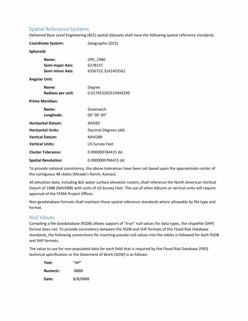
Spatial Reference Systems Delivered Base Level Engineering (BLE) spatial datasets shall have the following spatial reference standards.
Coordinate System: Geographic (GCS)
Spheroid:
Name: GRS_1980
Semi major Axis: 6378137
Semi minor Axis: 6356752.3141403561
Angular Unit:
Name: Degree
Radians per unit: 0.017453292519943299
Prime Meridian:
Name: Greenwich
Longitude: 00° 00’ 00”
Horizontal Datum: NAD83
Horizontal Units: Decimal Degrees (dd)
Vertical Datum: NAVD88
Vertical Units: US Survey Feet
Cluster Tolerance: 0.000000784415 dd
Spatial Resolution: 0.0000000784415 dd
To provide national consistency, the above tolerances have been set based upon the approximate center of
the contiguous 48 states (Meade’s Ranch, Kansas).
All elevation data, including BLE water surface elevation rasters, shall reference the North American Vertical
Datum of 1988 (NAVD88) with units of US Survey Feet. The use of other datums or vertical units will require
approval of the FEMA Project Officer.
Non‐geodatabase formats shall maintain these spatial reference standards where allowable by file type and
format.
Null Values Compiling a file Geodatabase (fGDB) allows support of “true” null values for data types, the shapefile (SHP)
format does not. To provide consistency between the fGDB and SHP formats of the Flood Risk Database
standards, the following conventions for inserting pseudo null values into the tables is followed for both fGDB
and SHP formats.
The value to use for non‐populated data for each field that is required by the Flood Risk Database (FRD)
technical specification or the Statement of Work (SOW) is as follows:
Text: “NP”
Numeric: ‐8888
Date: 8/8/8888

The value to use for fields that are optional or required when applicable either by the FRD technical
specification or the SOW is as follows:
Text: Null (or “”, the empty string)
Numeric: ‐9999
Date: 9/9/9999
For raster data, the value ‘NODATA’ should be used to represent the absence of data or null values.
Generally, all areas outside the project area (i.e., the polygon in S_FRD_Proj_Ar) will be set to ‘NODATA’ in
the depth and analysis rasters.
Topology Rules Vector data files must meet the following data structure requirements:
Digitized linework must be collected at a reasonably fine line weight.
Only simple point, polyline, and polygon elements may be used. Multi‐part features are not allowed.
Line features must be continuous (no dashes, dots, patterns or hatching).
Spatial files must not contain any linear or area patterns.
Area spatial features for a given theme must cover the entire BLE Project area without overlaps or silver polygons between adjacent polygons. Gaps or overshoots between features that should close must be eliminated.
Spatial Layer Topology Rule Minimum Cluster Tolerance (dd)
Line_Feature Must Be Larger Than Cluster Tolerance 0.000000784415
Line_Feature Must Not Overlap 0.000000784415
Line_Feature Must Be Single Part 0.000000784415
Line_Feature Must Not Self‐Intersect 0.000000784415
Line_Feature Must Not Self‐Overlap 0.000000784415
Polygon_Feature Must Be Larger Than Cluster Tolerance 0.000000784415
Spatial Layer Topology Rule Minimum Cluster Tolerance (dd)
Polygon_Feature Must Not Overlap 0.000000784415
Polygon_Feature Must Not Have Gaps 0.000000784415

HUC8_StatusInfo This polygon feature class is used to visualize the status for planned, in progress and completed Base Level
Engineering assessments completed within the Region. This feature class is maintained and updated by the
RSC. The REST service is available:
(https://maps103.halff.com/chimera/rest/services/FEMAr6rsc/BLE_Watersheds/MapServer).
Required: Yes, information is visualized on the Estimated BFE Viewer. Data is submitted via email to
the Regional Support Center.
Exceptions: None
Viewer Requirements: Mapping Partners shall coordinate with the RSC to assure the proper status is
depicted on the Estimated BFE Viewer.
In order to maintain the HUC8 Status on the viewer, Mapping Partners shall follow coordination instructions
below:
Update 1 – Project Start ‐ Add BLE Watershed to Viewer
When a Base Level Engineering project is initiated, Mapping Partners shall provide the following data via
email to the RSC for inclusion in the dataset. Mapping Partners should email [email protected] and cc their
FEMA Project Monitor.
HUC8 Provide the 8‐digit HUC8 number (i.e. 12060102)
Name Provide the HUC8 watershed name as indicated in the NHD Watershed Boundary
Dataset (i.e. Upper Clear Fork Brazos)
Status Choose from the following: Planned, In Progress, Complete
BLE Delivery Provide Target BLE Data Delivery Date (MM/DD/YYYY format)
Note: Date on viewer will be Target + 30 days to allow for review/upload
Update 2 – Update Delivery Date
Once the project is underway, the FEMA Project Monitor, CTP Lead or Mapping Partner should provide
updates to Matt Lepinski ([email protected]) if the Base Level Engineering delivery dates shift.
Update 3 – Alert FEMA Region 6 (and
RPML) of pending Data Submittal for
Review
When the BLE deliverables are nearly
ready for submittal, the Mapping Partner
shall alert Matthew Lepinski
([email protected]) with
FEMA Region 6, and the Regional
Program Management Lead (RPML),
Elizabeth Savage ([email protected])
that that a watershed, or other project
area is nearing completion.
Data should be delivered to FEMA and
the RPML via hard drive or eFTP site for
review. FEMA may request the
assistance of the RSC, who will perform a
completeness check of the dataset. At
the same time, FEMA R6 will review the
information to assure that submitted files
and datasets meet all requirements for loading the models, reports and spatial information to the viewer.
Figure 3: Base Level Engineering Project Status

Mapping Partners should consult the tips and tricks within this document prior to submitting a BLE dataset to
assure the spatial reviews identified within are performed. This will reduce the number of comments and
speed up the data load of the BLE data (models, report and spatial) onto the Estimated BFE Viewer site.
HUC10_ModelInfo This polygon feature class catalogs the data availability and location of HEC‐RAS model information once Base
Level Engineering models have been delivered through the Mapping Information Platform. This file leverages
the HUC10 sub‐basins developed and included in the NHD Watershed Boundary Dataset and provides URL
information for inclusion in the automated Detailed Report prepared by the Estimated BFE Viewer.
This polygon feature class is maintained and updated by the RSC. The REST Service is available:
(https://maps103.halff.com/chimera/rest/services/FEMAr6rsc/BLE_Watersheds/MapServer).
Required: Yes, information is queried and included in the Detailed Report prepared by the Estimated
BFE Viewer. Data is submitted via email, using table below, to RSC ([email protected]).
Exceptions: None
Viewer Requirements: Mapping Partners shall coordinate with the RSC once Base Level Engineering data is
delivered to the MIP. Mapping Partners will need to provide a shortened path for
each set of HEC‐RAS models delivered by HUC10.
To provide the user the location of the modeling files on the MIP for inclusion in the HUC10 coverage
maintained by the RSC, Mapping Partners shall prepare the table below and include in Update 3 email
(project status) sent to the RSC.
HUC8 12060102 Upper Clear Fork Brazos
BLE Data Complete 04/30/2017
Hydraulic Model Data Location on the MIP
HUC10 Name Model_Loc
1206010201 Linn K:/FY2016/16‐06‐3600S/Hydraulics ‐ Fisher County, TX ‐ 1/Hydraulic Data Capture ‐ Hydraulic Data Capture 48151C ‐ 1/Hydraulic_Models/Linn
1206010202 Headwaters K:/FY2016/16‐06‐3600S/Hydraulics ‐ Fisher County, TX ‐ 1/Hydraulic Data Capture ‐ Hydraulic Data Capture 48151C ‐ 1/Hydraulic_Models/Headwaters
Mapping Partners will need to support the RSC in providing the location of the hydraulic models by HUC10 by
providing a shortened URL for inclusion in the data service maintained by the RSC. The URL should be
shortened as shown below. If the URL is not shortened, it will not fit within the report area and may run off
the page. An example of how to shorten the URL is described below.
MIP Project Path: K:/FY2016/16-06-3600S/Hydraulics - Fisher County, TX - 1/Hydraulic Data Capture - Hydraulic Data Capture 48151C - 1/Hydraulic_Models/Linn
Remove/Adjust: K:/R06/TEXAS_48/FISHER_48151/FISHER_151C/16-06-3600S/ SubmissionRepository/Hydraulics/2186733/Hydraulic_Models/Linn
Shorten to: (Name) K:/R06/TX/Fisher/16‐06‐3600S/Hydraulics/Models/Linn
(HUC10 Number) K:/R06/TX/Fisher/16‐06‐3600S/Hydraulics/Models/1206010201
State Abbreviation County Name
Hydraulics/Models

S_Pol_AR This polygon feature class combines any information available in modernized DFIRM Database S_POL_AR
feature class for the project area. The Mapping Partner shall compile the polygon feature class to include
one record (polygon) per community. This will require the use of multi‐part polygons for non‐contiguous
community boundaries/areas.
This dataset is described in detail within the Flood Insurance Rate Map (FIRM) Database Technical Reference:
Preparing Flood Insurance Rate Map Databases (Feb 2018), Page 66 (Feature Class: S_Pol_Ar). Mapping
Partners shall follow the instructions within the Technical Reference for the compilation of this dataset.
Note (April 2019): The S_Pol_AR dataset replaces the historic submittal of the FRC_Pol_AR dataset and
L_RA_Results table within the Spatial deliverables for each BLE submittal.
Required: Yes, minimum deliverable for 1‐D and 2‐D BLE analysis areas. The S_Pol_AR feature class
shall be compiled for the study area, but no larger than one (1) HUC8 watershed per delivery
area.
Exceptions: Mapping Partners may decide to leave community polygons complete instead of clipping
them to the project boundary. Leaving the community boundaries complete and intact will
support the preparation of Community Dashboards when the Flood Risk Report is being
compiled.
Inclusions: No additional data elements (columns) have been added to this dataset.
Viewer Requirements: None. Layer not used in Estimated BFE Viewer.
Figure 4: Example S_Pol_AR
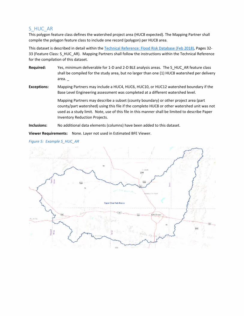
S_HUC_AR This polygon feature class defines the watershed project area (HUC8 expected). The Mapping Partner shall
compile the polygon feature class to include one record (polygon) per HUC8 area.
This dataset is described in detail within the Technical Reference: Flood Risk Database (Feb 2018), Pages 32‐
33 (Feature Class: S_HUC_AR). Mapping Partners shall follow the instructions within the Technical Reference
for the compilation of this dataset.
Required: Yes, minimum deliverable for 1‐D and 2‐D BLE analysis areas. The S_HUC_AR feature class
shall be compiled for the study area, but no larger than one (1) HUC8 watershed per delivery
area. _
Exceptions: Mapping Partners may include a HUC4, HUC6, HUC10, or HUC12 watershed boundary if the
Base Level Engineering assessment was completed at a different watershed level.
Mapping Partners may describe a subset (county boundary) or other project area (part
county/part watershed) using this file if the complete HUC8 or other watershed unit was not
used as a study limit. Note, use of this file in this manner shall be limited to describe Paper
Inventory Reduction Projects.
Inclusions: No additional data elements (columns) have been added to this dataset.
Viewer Requirements: None. Layer not used in Estimated BFE Viewer.
Figure 5: Example S_HUC_AR

SUBBASINS
SUB‐BASINS This polygon feature class collects data and calculations used in the preparation of Base Level Engineering hydrology, which uses the Regional Regression
Equations to calculate the flow volumes expected throughout study reaches.
This dataset leverages the DFIRM database S_SUB‐BASINS feature class described in Flood Insurance Rate Map (FIRM) Database Technical Reference:
Preparing Flood Insurance Rate Map Databases (Feb 2018), Pages 74‐76 (Feature Class: S_SUB‐BASINS). Mapping Partners shall follow the instructions
within the Technical Reference for the compilation of this dataset elements described within.
Required: Yes, minimum deliverable for 1‐D analysis. The S_SUB‐BASINS feature class shall be compiled for the study area, but no larger than one
(1) HUC8 watershed per delivery area.
Exceptions: Not required for delivery in 2‐D BLE analysis watersheds.
Inclusions: Additional feature information related to basin area, basin slope, upstream basins, downstream basins are expected for BLE assessment
areas, additional data requirements outlined in the table below.
Viewer Requirements: Layer not used in Estimated BFE Viewer.
EBFE Database Data Element
DFIRM Database Data Element
Description
EST_ID DFIRM_ID Study Identifier: Suggest HUC8 (or other be used) to define the study area – I.E. 12060102_BLE
VERSION_ID VERSION_ID Version Identifier ‐ Identifies the product version and relates the feature to standards according to how it was created (Suggest BLE_MMYYYY)
E_SUBAS_ID SUBBAS_ID Primary key for table lookup. Assigned by table creator
HUC8_CODE HUC8 USGS HUC8 code number of sub‐basin
E_SUBAS_NM SUBBAS_NM Name of sub‐basin
EST_AREA SUB_AREA Area of sub‐basin
AREA_UNIT AREA_UNIT Area Units ‐ Indicates the measurement system used for the basins. Use values in D_Area_Units.
US_1 NEW Field Upstream basin 1
US_2 NEW Field Upstream basin 2
US_3 NEW Field Upstream basin 3
US_4 NEW Field Upstream basin 4
DS_1 NEW Field Downstream basin
PRECIP_IN NEW Field Precipitation in inches
MAINCHSLP NEW Field Main channel slope of basin
E_Q_10PCT NEW Field Flow calculated for the 10% Flood

SUBBASINS
EBFE Database Data Element
DFIRM Database Data Element
Description
E_Q_04PCT NEW Field Flow calculated for the 4% Flood
E_Q_02PCT NEW Field Flow calculated for the 2% Flood
E_Q_01PCT NEW Field Flow calculated for the 1% Flood
E_Q_01PLUS NEW Field Flow calculated for the 1%+ Flood
E_Q_01MIN NEW Field Flow calculated for the 1%‐ Flood
E_Q_0_2PCT NEW Field Flow calculated for the 0.2% Flood
SOURCE_CIT SOURCE_CIT Abbreviation used in the metadata file when describing the source information for the feature
These fields will remain in geodatabase but will be hidden.
HIDE WTR_NM Surface water feature name
HIDE BASIN_DESC Sub‐basin description
HIDE NODE_ID Node Identification
HIDE BASIN_TYP Type of Sub‐basin
Figure 6: Example S_SUB‐BASINS

XS
XS_1D This polyline feature class depicts the location and orientation of the analysis cross‐sections used to determine the Base Level Engineering hydraulic
modeling.
This dataset leverages the DFIRM database S_XS feature class described in Flood Insurance Rate Map (FIRM) Database Technical Reference: Preparing
Flood Insurance Rate Map Databases (Feb 2018), Pages 87‐90 (Feature Class: S_XS). Mapping Partners shall follow the instructions within the Technical
Reference for the compilation of this dataset elements described within.
Required: Yes, minimum deliverable for 1‐D analysis. The XS feature class shall be compiled for the study area but should be no larger than one (1)
HUC8 watershed per delivery area.
Exceptions: Not required for delivery in 2‐D BLE analysis watersheds.
Inclusions: Additional feature information to describe the calculated flow values and estimated Base Flood Elevation at each of the seven
frequencies have been added to the S_XS fields for reference.
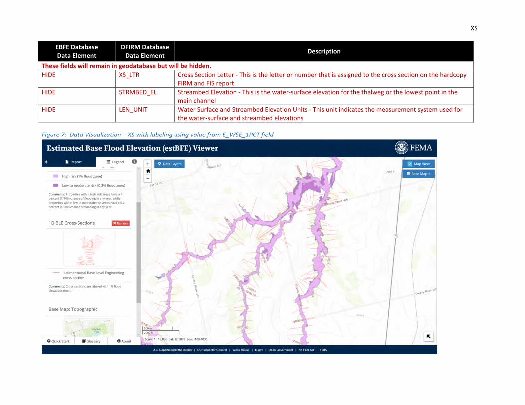
Viewer Requirements: The field labeled E_WSE_1PCT will be used to label cross‐sections on the viewer. The water surface elevations loaded to the
seven WSEL fields should be included to the nearest tenth of a foot (0.0 ft) when loaded into the database.
Mapping Partners shall review the stream WSEL profile of the 1% annual chance water surface elevations to determine which
cross‐sections should be visualized on the Estimated BFE Viewer tool. Providers shall update the XS_LN_TYP field to indicate the
cross‐sections as “MAPPED” to indicate which of the cross‐sections will be visible on the Estimated BFE Viewer tool.
Each cross‐section in backwater shall be indicated as “NOT MAPPED” in the XS_LN_TYP field.
Cross‐sections at inflection points along the water surface elevation profile should be indicated as “MAPPED”
A “MAPPED” cross‐section should be included at least every 2,500 ft along the stream centerline to support community
use of the tool and datasets.
NOTE – All prepared BLE WSEL grids MUST include backwater effects even though E_WSE_1PCT attribute in the XS file is
not required to include backwater.
XS
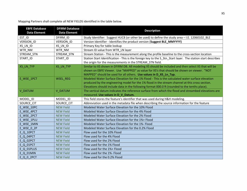
Mapping Partners shall complete all NEW FIELDS identified in the table below.
EBFE Database Data Element
DFIRM Database Data Element
Description
EST_ID DFIRM_ID Study Identifier: Suggest HUC8 (or other be used) to define the study area – I.E. 12060102_BLE
VERSION_ID VERSION_ID Version Identifier ‐ Identifies the product version (Suggest BLE_MMYYYY)
XS_LN_ID XS_LN_ID Primary Key for table lookup
WTR_NM WTR_NM Stream ID value from WTR_LN layer
STREAM_STN STREAM_STN Stream Station ‐ This is the measurement along the profile baseline to the cross‐section location
START_ID START_ID Station Start Identification ‐ This is the foreign key to the S_Stn_Start layer. The station start describes the origin for the measurements in the STREAM_STN field.
XS_LN_TYP XS_LN_TYP Similar to XS shown in DFIRM DB. All modeling XS should be included and then select XS that will be shown on EBFE Viewer. Use "MAPPED" as value for XS's that should be shown on viewer. "NOT MAPPED" should be used for all others. Use values in D_XS_Ln_Typ.
E_WSE_1PCT WSEL_REG Modeled Water Surface Elevation for the 1% Flood ‐ This is the calculated water surface elevation produced by the engineering model for the 1% flood in the stream channel at this cross section. Elevations should include data in the following format 000.0 ft (rounded to the tenths place).
V_DATUM V_DATUM The vertical datum indicates the reference surface from which the flood and streambed elevations are measured. Use values in D_V_Datum.
MODEL_ID MODEL_ID This field stores the feature's identifier that was used during H&H modeling.
SOURCE_CIT SOURCE_CIT Abbreviation used in the metadata file when describing the source information for the feature
E_WSE_10PC NEW Field Modeled Water Surface Elevation for the 10% Flood
E_WSE_4PCT NEW Field Modeled Water Surface Elevation for the 4% Flood
E_WSE_2PCT NEW Field Modeled Water Surface Elevation for the 2% Flood
E_WSE_1PLU NEW Field Modeled Water Surface Elevation for the 1%+ Flood
E_WSE_1MIN NEW Field Modeled Water Surface Elevation for the 1%‐ Flood
E_WSE_0_2P NEW Field Modeled Water Surface Elevation for the 0.2% Flood
E_Q_10PCT NEW Field Flow used for the 10% Flood
E_Q_04PCT NEW Field Flow used for the 4% Flood
E_Q_02PCT NEW Field Flow used for the 2% Flood
E_Q_01PCT NEW Field Flow used for the 1% Flood
E_Q_01PLUS NEW Field Flow used for the 1%+ Flood
E_Q_01MIN NEW Field Flow used for the 1%‐ Flood
E_Q_0_2PCT NEW Field Flow used for the 0.2% Flood
XS
EBFE Database Data Element
DFIRM Database Data Element
Description
These fields will remain in geodatabase but will be hidden.
HIDE XS_LTR Cross Section Letter ‐ This is the letter or number that is assigned to the cross section on the hardcopy FIRM and FIS report.
HIDE STRMBED_EL Streambed Elevation ‐ This is the water‐surface elevation for the thalweg or the lowest point in the main channel
HIDE
LEN_UNIT Water Surface and Streambed Elevation Units ‐ This unit indicates the measurement system used for the water‐surface and streambed elevations
Figure 7: Data Visualization – XS with labeling using value from E_WSE_1PCT field

BFE
BFE_2D This polyline feature class depicts whole foot elevations of the 1%‐annual‐chance‐flood resulting from a 2‐D Base Level Engineering analysis.
This dataset leverages the DFIRM database S_BFE feature class described in Flood Insurance Rate Map (FIRM) Database Technical Reference: Preparing
Flood Insurance Rate Map Databases (Feb 2018), Pages 22‐24 (Feature Class: S_BFE). Mapping Partners shall follow the instructions within the Technical
Reference for the compilation of this dataset elements described within and review the additional guidance to assure the datasets will be correctly
compiled for use and upload to the Estimated BFE Viewer.
Required: Yes, minimum deliverable for 2‐D analysis. The BFE feature class shall be compiled for the study area, but no larger than one (1) HUC8
watershed per delivery area.
Exceptions: Not required for delivery in 1‐D BLE analysis watersheds.
Inclusions: None.
Viewer Requirements: BFE lines shall be loaded into the BFE feature class. Viewer requires the Mapping Partner to complete the field BLELEV1PCT with
the whole foot elevation of the 1‐percent‐annual‐chance event.
The field labeled BLELEV1PCT will be used to label the BFE lines on the viewer. The water surface elevation contours
should be generated at a one‐foot contour interval.
Mapping Partners shall prepare a BFE line file leveraging the 1‐percent annual chance water surface elevation grid
prepared during the Base Level Engineering watershed assessment.
Mapping Partners shall complete all NEW FIELDS identified in the table below.
EBFE Database Data Element
DFIRM Database Data Element
Description
EST_ID DFIRM_ID Study Identifier ‐ Consists of State FIPS Code, County FIPS Code, and the Letter "C". E.G. 48107C (Suggest HUC8# be included)
VERSION_ID VERSION_ID Version Identifier ‐ Identifies the product version and relates the feature to standards according to how it was created (Suggest BLE_MMYYYY)
EBFE_LN_ID BFE_LN_ID Primary Key for table lookup.
BLELEV1PCT ELEV The rounded, whole‐foot elevation of the 1‐percent‐annual‐chance flood. This is the value of the BFE that is shown next to the BFE line in the viewer.
BFE_LN_TYP BFE_LN_TYP Similar to XS shown in DFIRM DB. All modeling XS should be included and then select XS that will be shown on EBFE Viewer. Use "MAPPED" as value for XS's that should be shown on viewer. "NOT MAPPED" should be used for all others. Use values in D_XS_Ln_Typ.
LEN_UNIT LEN_UNIT Length Units ‐ Indicates the measurement system used for the BFEs and/or depths. Use values in D_Length_Units.

BFE
EBFE Database Data Element
DFIRM Database Data Element
Description
V_DATUM V_DATUM Vertical Datum ‐ Indicates the reference surface from which the flood elevations are measured. Use values in D_V_Datum.
SOURCE_CIT SOURCE_CIT Abbreviation used in the metadata file when describing the source information for the feature
Figure 8: Data Visualization – BFE_2D with labeling using value from E_WSE_1PCT field (site labels each 10‐foot increment at this time)
60’ elevation is labeled, but each contour (brown) represents 1‐foot elevation change

WTR_LN
WTR_LN This polyline feature class depicts the location of stream centerlines used in hydrologic and hydraulic analysis.
This dataset leverages the DFIRM database S_WTR_LN feature class described in Flood Insurance Rate Map (FIRM) Database Technical Reference:
Preparing Flood Insurance Rate Map Databases (Feb 2018), Pages 85‐87 (Feature Class: S_WTR_LN). Mapping Partners shall follow the instructions within
the Technical Reference for the compilation of this dataset elements described within.
Required: Yes, minimum deliverable for 1‐D and 2‐D BLE analysis areas. The WTR_LN feature class shall be compiled for the study area, but no
larger than one (1) HUC8 watershed per delivery area.
Exceptions: None.
Inclusions: None.
Viewer Requirements: The field WTR_NM will be used to label the stream centerline in the image in the detailed report. This field should be
completed for all Base Level Engineering streams studied. Mapping Partners may determine their own labeling system
(numbering 1.1.1, or naming Tributary 1 to Stream), but should be consistent and should assure that model delivery through the
MIP uses the same naming convention to support MSC staff in providing the appropriate and correct model when requested.
EBFE Database Data Element
DFIRM Database Data Element
Description
EST_ID DFIRM_ID Study Identifier: Suggest HUC8 (or other be used) to define the study area – I.E. 12060102_BLE
VERSION_ID VERSION_ID Version Identifier ‐ Identifies the product version (Suggest BLE_MMYYYY)
WTR_LN_ID WTR_LN_ID Primary key for table lookup. Assigned by table creator
WTR_NM WTR_NM Surface Water Feature Name Formal name of the water feature as it will appear in the Estimated BFE Viewer Detailed Report.
SOURCE_CIT SOURCE_CIT Abbreviation used in the metadata file when describing the source information for the feature
These fields will remain in geodatabase but will be hidden.
HIDE SHOWN_FIRM Shown on FIRM. If the water feature is shown on the FIRM this field is "True"
HIDE SHOWN_INDX Shown on Index Map ‐ If the water feature is shown on the Index Map this field would be "True"

WTR_AR
WTR_AR This polyline feature class depicts the location of water bodies throughout the study area.
This dataset leverages the DFIRM database S_WTR_AR feature class described in Flood Insurance Rate Map (FIRM) Database Technical Reference:
Preparing Flood Insurance Rate Map Databases (Feb 2018), Pages 84‐85 (Feature Class: S_WTR_AR). Mapping Partners shall follow the instructions within
the Technical Reference for the compilation of this dataset elements described within.
Required: Yes, minimum deliverable, no matter which analysis approach (1‐D or 2‐D) is used. The WTR_AR feature class shall be compiled for the
study area, but no larger than one (1) HUC8 watershed per delivery area.
Exceptions: None.
Inclusions: None.
Viewer Requirements: None.
EBFE Database Data Element
DFIRM Database Data Element
Description
EST_ID DFIRM_ID Study Identifier: Suggest HUC8 (or other be used) to define the study area – I.E. 12060102_BLE
VERSION_ID VERSION_ID Version Identifier ‐ Identifies the product version (Suggest BLE_MMYYYY)
WTR_AR_ID WTR_AR_ID Primary key for table lookup. Assigned by table creator
WTR_NM WTR_NM Surface Water Feature Name ‐ Formal name of the water feature as it will appear on the hardcopy FIRM.
SOURCE_CIT SOURCE_CIT Abbreviation used in the metadata file when describing the source information for the feature
These fields will remain in geodatabase but will be hidden.
HIDE SHOWN_FIRM Shown on FIRM. If the water feature is shown on the FIRM this field is "True"
HIDE SHOWN_INDX Shown on Index Map ‐ If the water feature is shown on the Index Map this field would be "True"
DTL_STUD_LN
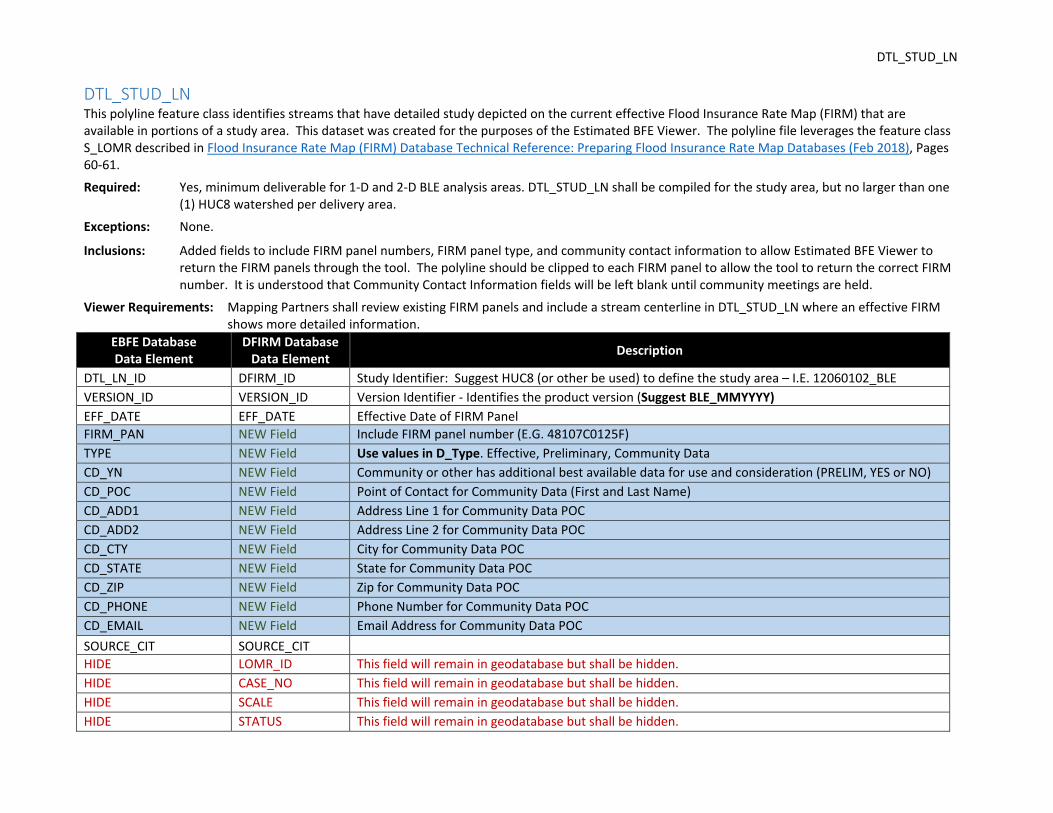
DTL_STUD_LN This polyline feature class identifies streams that have detailed study depicted on the current effective Flood Insurance Rate Map (FIRM) that are available in portions of a study area. This dataset was created for the purposes of the Estimated BFE Viewer. The polyline file leverages the feature class S_LOMR described in Flood Insurance Rate Map (FIRM) Database Technical Reference: Preparing Flood Insurance Rate Map Databases (Feb 2018), Pages 60‐61.
Required: Yes, minimum deliverable for 1‐D and 2‐D BLE analysis areas. DTL_STUD_LN shall be compiled for the study area, but no larger than one (1) HUC8 watershed per delivery area.
Exceptions: None.
Inclusions: Added fields to include FIRM panel numbers, FIRM panel type, and community contact information to allow Estimated BFE Viewer to return the FIRM panels through the tool. The polyline should be clipped to each FIRM panel to allow the tool to return the correct FIRM number. It is understood that Community Contact Information fields will be left blank until community meetings are held.
Viewer Requirements: Mapping Partners shall review existing FIRM panels and include a stream centerline in DTL_STUD_LN where an effective FIRM shows more detailed information.
EBFE Database Data Element
DFIRM Database Data Element
Description
DTL_LN_ID DFIRM_ID Study Identifier: Suggest HUC8 (or other be used) to define the study area – I.E. 12060102_BLE
VERSION_ID VERSION_ID Version Identifier ‐ Identifies the product version (Suggest BLE_MMYYYY)
EFF_DATE EFF_DATE Effective Date of FIRM Panel
FIRM_PAN NEW Field Include FIRM panel number (E.G. 48107C0125F)
TYPE NEW Field Use values in D_Type. Effective, Preliminary, Community Data
CD_YN NEW Field Community or other has additional best available data for use and consideration (PRELIM, YES or NO)
CD_POC NEW Field Point of Contact for Community Data (First and Last Name)
CD_ADD1 NEW Field Address Line 1 for Community Data POC
CD_ADD2 NEW Field Address Line 2 for Community Data POC
CD_CTY NEW Field City for Community Data POC
CD_STATE NEW Field State for Community Data POC
CD_ZIP NEW Field Zip for Community Data POC
CD_PHONE NEW Field Phone Number for Community Data POC
CD_EMAIL NEW Field Email Address for Community Data POC
SOURCE_CIT SOURCE_CIT
HIDE LOMR_ID This field will remain in geodatabase but shall be hidden.
HIDE CASE_NO This field will remain in geodatabase but shall be hidden.
HIDE SCALE This field will remain in geodatabase but shall be hidden.
HIDE STATUS This field will remain in geodatabase but shall be hidden.

DTL_STUD_AR
DTL_STUD_AR This polygon feature class identifies areas that have detailed study depicted on the current effective Flood Insurance Rate Map (FIRMs) that are available
in portions of a study area. The polygon file leverages the feature class S_LOMR described in Flood Insurance Rate Map (FIRM) Database Technical
Reference: Preparing Flood Insurance Rate Map Databases (Feb 2018), Pages 60‐61. This dataset was created for the purposes of the Estimated BFE
Viewer.
Required: Yes, minimum deliverable, no matter which analysis approach (1‐D or 2‐D) is used. DTL_STUD_AR shall be compiled for the study area,
but no larger than one (1) HUC8 watershed per delivery area.
Exceptions: None.
Inclusions: Added fields to include FIRM panel numbers, FIRM panel type, and community contact information to allow Estimated BFE
Viewer to return the FIRM panels through the tool. The polygon should be clipped to each FIRM panel to allow the tool to
return the correct FIRM number. It is understood that Community Contact Information fields will be left blank until community
meetings are held.
Viewer Requirements: Mapping Partners shall review existing FIRM panels and include an area in DTL_STUD_AR where an effective FIRM shows more
detailed information.
Mapping Partners should prepare a polygon to bound the existing detailed floodplains depicted on the FIRMs.
EBFE Database Data Element
DFIRM Database Data Element
Description
DTL_AR_ID DFIRM_ID Study Identifier – Suggest HUC8 (or other be used) to define the study area – I.E. 12060102_BLE
VERSION_ID VERSION_ID Version Identifier ‐ Identifies the product version (Suggest BLE_MMYYYY)
EFF_DATE EFF_DATE Effective Date of FIRM Panel
FIRM_PAN NEW Field Include FIRM panel number (E.G. 48107C0125F)
TYPE NEW Field Use values in D_Type. (Effective, Preliminary, or Community Data)
CD_YN NEW Field Community or other has additional best available data for use and consideration (PRELIM, YES or NO)
CD_POC NEW Field Point of Contact for Community Data (First and Last Name)
CD_ADD1 NEW Field Address Line 1 for Community Data POC
CD_ADD2 NEW Field Address Line 2 for Community Data POC
CD_CTY NEW Field City for Community Data POC
CD_STATE NEW Field State for Community Data POC
CD_ZIP NEW Field Zip for Community Data POC
CD_PHONE NEW Field Phone Number for Community Data POC
CD_EMAIL NEW Field Email Address for Community Data POC

DTL_STUD_AR
SOURCE_CIT SOURCE_CIT
EBFE Database Data Element
DFIRM Database Data Element
Description
HIDE LOMR_ID This field will remain in geodatabase but shall be hidden.
HIDE CASE_NO This field will remain in geodatabase but shall be hidden.
HIDE SCALE This field will remain in geodatabase but shall be hidden.
HIDE STATUS This field will remain in geodatabase but shall be hidden.
Figure 9: Data Visualization – Detailed Study Streams and Detailed Study Areas
Detailed Study Area – Grey Polygon
Detailed Study Line – Blue Centerline

FLD_HAZ_AR
FLD_HAZ_AR This polygon feature class contains information about the flood hazards within the Flood Risk Project area. The spatial elements representing the flood
zones are polygons. The entire area of the jurisdiction(s) mapped by the FIRM should have a corresponding flood zone polygon. There is one polygon for
each contiguous flood zone designated.
This dataset leverages the DFIRM database S_FLD_HAZ_AR feature class described in Flood Insurance Rate Map (FIRM) Database Technical Reference:
Preparing Flood Insurance Rate Map Databases (Feb 2018), Pages 40‐46 (Feature Class: S_FLD_HAZ_AR). Mapping Partners shall follow the instructions
within the Technical Reference for the compilation of this dataset elements described within and review the additional guidance to assure the datasets
will be correctly compiled for use and upload to the Estimated BFE Viewer.
Required: Yes, minimum deliverable, no matter which analysis approach (1‐D or 2‐D) is used. The FLD_HAZ_AR feature class shall be compiled for
the study area, but no larger than one (1) HUC8 watershed per delivery area.
Exceptions: None.
Inclusions: Added a field FLD_RISK to allow inclusion of Moderate, or High flood risk evaluation. This value is returned in the report and in the
interactive use of the Estimated BFE Viewer.
Viewer Requirements: 1% floodplains and 0.2% floodplains shall be loaded into the FLD_HAZ_AR feature class.
Viewer requires the Mapping Partner to complete the field EST_RISK. A “moderate” value should be used for areas that are
within the 0.2% annual chance floodplain area, and “high” is associated with the areas within the 1% annual chance floodplain.
Domain table D_Fld_Risk should be used for these values.
Mapping Partner is NOT required to complete the FLD_ZONE field since the Base Level Engineering information is NOT updating
a FIRM when completed and compiled. If the Mapping Partner decides to complete this field the 1% annual chance polygon
should be labeled “A”, and the 0.2% annual chance polygon should be labeled “X”.
EBFE Database Data Element
DFIRM Database Data Element
Description
EST_ID DFIRM_ID Study Identifier ‐ Consists of State FIPS Code, County FIPS Code, and the Letter "C". E.G. 48107C (Suggest HUC8# be included)
VERSION_ID VERSION_ID Version Identifier ‐ Identifies the product version and relates the feature to standards according to how it was created (Suggest BLE_MMYYYY)
EST_AR_ID FLD_AR_ID Primary key for table lookup. Assigned by table creator
ZONE_SUBTY ZONE_SUBTY Flood Zone Subtype ‐ Captures additional information about the flood zones not related to insurance rating purposes

FLD_HAZ_AR
EBFE Database Data Element
DFIRM Database Data Element
Description
V_DATUM V_DATUM Vertical Datum ‐ Indicates the reference surface from which the flood elevations are measured. Use values in D_V_Datum.
LEN_UNIT LEN_UNIT Length Units ‐ Indicates the measurement system used for the BFEs and/or depths. Use values in D_Length_Units.
SOURCE_CIT SOURCE_CIT Abbreviation used in the metadata file when describing the source information for the feature
EST_Risk NEW Field "Moderate" ‐ 0.2% floodplain; "High" ‐ within 1% floodplain. Use values in D_Fld_Risk.
These fields will remain in geodatabase but will be hidden.
HIDE STUDY_TYP Study Type ‐ Describes the type of Flood Risk Project performed for flood hazard identification.
HIDE SFHA_TF Special Flood Hazard Area ‐ If the area is within an SFHA, this field is "True". If not, field is "False"
HIDE STATIC_BFE Static Base Flood Elevation ‐ Populated for areas that have been determined to have a constant BFE over a flood zone
HIDE DEPTH Depth for Zone AO areas
HIDE VELOCITY Velocity measurement of the flood flow in an area
HIDE VEL_UNIT Unit of measurement for the velocity
HIDE AR_REVERT If this area is Zone AR in FLD_Zone, this field would hold the zone that area would revert to if the AR zone were removed
HIDE AR_SUBTRV If this area is Zone AR in FLD_Zone, this field would hold the zone subtype that area would revert to if the AR zone were removed
HIDE BFE_REVERT Depth Revert ‐ If zone is a Zone AR in FLD_ZONE this field would hold the static base flood elevation for the reverted zone.
HIDE DEP_REVERT Depth Revert ‐ If zone is a Zone AR in FLD_ZONE this field would hold the flood depth for the reverted zone.
HIDE DUAL_ZONE Flood Control Restoration Zone ‐ Populated if the flood hazard areas shown on the effective FIRM will be designated as "duel" flood insurance rate zones
HIDE FLD_ZONE Not required ‐ Flood Zone designation

FLD_HAZ_AR
Figure 10: Data Visualization – Estimated Flood Extents (depicts the 1% and 0.2% annual chance events determined in Base Level Engineering assessment)
Light Purple – 1% annual chance HIGH Flood Risk
Darker Purple – 0.2% annual chance MODERATE FLOOD RISK
Hollow – All other areas
LOW Flood Risk
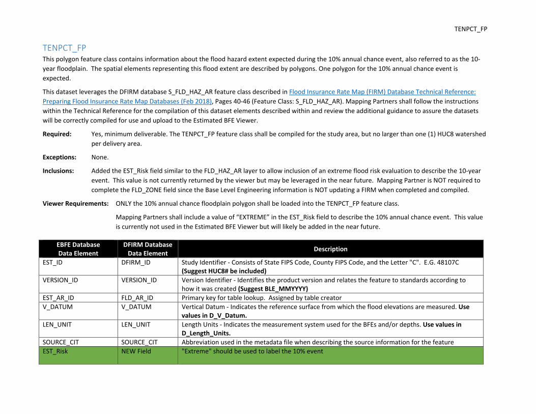
TENPCT_FP
TENPCT_FP This polygon feature class contains information about the flood hazard extent expected during the 10% annual chance event, also referred to as the 10‐
year floodplain. The spatial elements representing this flood extent are described by polygons. One polygon for the 10% annual chance event is
expected.
This dataset leverages the DFIRM database S_FLD_HAZ_AR feature class described in Flood Insurance Rate Map (FIRM) Database Technical Reference:
Preparing Flood Insurance Rate Map Databases (Feb 2018), Pages 40‐46 (Feature Class: S_FLD_HAZ_AR). Mapping Partners shall follow the instructions
within the Technical Reference for the compilation of this dataset elements described within and review the additional guidance to assure the datasets
will be correctly compiled for use and upload to the Estimated BFE Viewer.
Required: Yes, minimum deliverable. The TENPCT_FP feature class shall be compiled for the study area, but no larger than one (1) HUC8 watershed
per delivery area.
Exceptions: None.
Inclusions: Added the EST_Risk field similar to the FLD_HAZ_AR layer to allow inclusion of an extreme flood risk evaluation to describe the 10‐year
event. This value is not currently returned by the viewer but may be leveraged in the near future. Mapping Partner is NOT required to
complete the FLD_ZONE field since the Base Level Engineering information is NOT updating a FIRM when completed and compiled.
Viewer Requirements: ONLY the 10% annual chance floodplain polygon shall be loaded into the TENPCT_FP feature class.
Mapping Partners shall include a value of “EXTREME” in the EST_Risk field to describe the 10% annual chance event. This value
is currently not used in the Estimated BFE Viewer but will likely be added in the near future.
EBFE Database Data Element
DFIRM Database Data Element
Description
EST_ID DFIRM_ID Study Identifier ‐ Consists of State FIPS Code, County FIPS Code, and the Letter "C". E.G. 48107C (Suggest HUC8# be included)
VERSION_ID VERSION_ID Version Identifier ‐ Identifies the product version and relates the feature to standards according to how it was created (Suggest BLE_MMYYYY)
EST_AR_ID FLD_AR_ID Primary key for table lookup. Assigned by table creator
V_DATUM V_DATUM Vertical Datum ‐ Indicates the reference surface from which the flood elevations are measured. Use values in D_V_Datum.
LEN_UNIT LEN_UNIT Length Units ‐ Indicates the measurement system used for the BFEs and/or depths. Use values in D_Length_Units.
SOURCE_CIT SOURCE_CIT Abbreviation used in the metadata file when describing the source information for the feature
EST_Risk NEW Field "Extreme" should be used to label the 10% event

TENPCT_FP
EBFE Database Data Element
DFIRM Database Data Element
Description
These fields will remain in geodatabase but will be hidden.
HIDE STUDY_TYP Study Type ‐ Describes the type of Flood Risk Project performed for flood hazard identification.
HIDE SFHA_TF Special Flood Hazard Area ‐ If the area is within an SFHA, this field is "True". If not, field is "False"
HIDE ZONE_SUBTY Flood Zone Subtype ‐ Captures additional information about the flood zones not related to insurance rating purposes
HIDE STATIC_BFE Static Base Flood Elevation ‐ Populated for areas that have been determined to have a constant BFE over a flood zone
HIDE DEPTH Depth for Zone AO areas
HIDE VELOCITY Velocity measurement of the flood flow in an area
HIDE VEL_UNIT Unit of measurement for the velocity
HIDE AR_REVERT If this area is Zone AR in FLD_Zone, this field would hold the zone that area would revert to if the AR zone were removed
HIDE AR_SUBTRV If this area is Zone AR in FLD_Zone, this field would hold the zone subtype that area would revert to if the AR zone were removed
HIDE BFE_REVERT Depth Revert ‐ If zone is a Zone AR in FLD_ZONE this field would hold the static base flood elevation for the reverted zone.
HIDE DEP_REVERT Depth Revert ‐ If zone is a Zone AR in FLD_ZONE this field would hold the flood depth for the reverted zone.
HIDE DUAL_ZONE Flood Control Restoration Zone ‐ Populated if the flood hazard areas shown on the effective FIRM will be designated as "duel" flood insurance rate zones
HIDE FLD_ZONE Not Required ‐ Flood Zone ‐ 10‐year event boundary (Label 10% event)
Figure 11: Data Visualization –
10% Estimated Flood Extents
(depicts the 10% annual chance event
flood extent)
Lightest purple hue shows area where

BLE_WSE0_2PCT
BLE_WSE01PCT This raster dataset class contains the water surface elevation (WSEL) for the 1% annual chance event determined during the Base Level Engineering
assessment. This dataset leverages the Raster Dataset guidance described in Flood Risk Database (FRD) Technical Reference (Feb 2018), Section 4.0
Raster Datasets, Pages 74‐76.
Required: Yes, minimum deliverable for 1‐D and 2‐D BLE analysis areas. The BLE_WSE01PCT grid shall be compiled for the study area, but no larger
than one (1) HUC8 watershed per delivery area.
Exceptions: None.
Inclusions: None.
Viewer Requirements: ONLY the calculated 1% annual chance water surface elevation shall be included in this dataset as the grid value.
Mapping Partners will need to assure that grids have been adjusted to include any backwater effects from larger streams near
each confluence area.
Mapping Partners shall calculate the grid value to the tenths place (0.0 feet).
Mapping Partners shall not use a grid cell size any larger than 10 foot by 10 foot.
Mapping Partners shall clip the gridded information to match the extent of the 1% annual chance floodplain.
The 1% annual chance water surface elevation is leveraged by the Estimated BFE Viewer to return a value to the user for the estimated base flood
elevation at any location selected within the 1% annual chance event floodplain.

BLE_WSE0_2PCT
BLE_WSE0_2PCT This raster dataset class contains the water surface elevation (WSEL) for the 0.2% annual chance event determined during the Base Level Engineering
assessment. This dataset leverages the Raster Dataset guidance described in Flood Risk Database (FRD) Technical Reference (Feb 2018), Section 4.0
Raster Datasets, Pages 74‐76.
Required: Yes, minimum deliverable for 1‐D and 2‐D BLE analysis areas. The BLE_WSE0_2PCT grid shall be compiled for the study area, but no
larger than one (1) HUC8 watershed per delivery area.
Exceptions: None.
Inclusions: None.
Viewer Requirements: ONLY the calculated 0.2% annual chance water surface elevation shall be included in this dataset as the grid value.
Mapping Partners will need to assure that grids have been adjusted to include any backwater effects from larger streams near
each confluence area.
Mapping Partners shall calculate the grid value to the tenths place (0.0 feet).
Mapping Partners shall not use a grid cell size any larger than 10 foot by 10 foot.
Mapping Partners shall clip the gridded information to match the extent of the 0.2% annual chance floodplain.
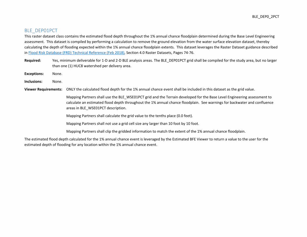
BLE_DEP0_2PCT
BLE_DEP01PCT This raster dataset class contains the estimated flood depth throughout the 1% annual chance floodplain determined during the Base Level Engineering
assessment. This dataset is compiled by performing a calculation to remove the ground elevation from the water surface elevation dataset, thereby
calculating the depth of flooding expected within the 1% annual chance floodplain extents. This dataset leverages the Raster Dataset guidance described
in Flood Risk Database (FRD) Technical Reference (Feb 2018), Section 4.0 Raster Datasets, Pages 74‐76.
Required: Yes, minimum deliverable for 1‐D and 2‐D BLE analysis areas. The BLE_DEP01PCT grid shall be compiled for the study area, but no larger
than one (1) HUC8 watershed per delivery area.
Exceptions: None.
Inclusions: None.
Viewer Requirements: ONLY the calculated flood depth for the 1% annual chance event shall be included in this dataset as the grid value.
Mapping Partners shall use the BLE_WSE01PCT grid and the Terrain developed for the Base Level Engineering assessment to
calculate an estimated flood depth throughout the 1% annual chance floodplain. See warnings for backwater and confluence
areas in BLE_WSE01PCT description.
Mapping Partners shall calculate the grid value to the tenths place (0.0 feet).
Mapping Partners shall not use a grid cell size any larger than 10 foot by 10 foot.
Mapping Partners shall clip the gridded information to match the extent of the 1% annual chance floodplain.
The estimated flood depth calculated for the 1% annual chance event is leveraged by the Estimated BFE Viewer to return a value to the user for the
estimated depth of flooding for any location within the 1% annual chance event.
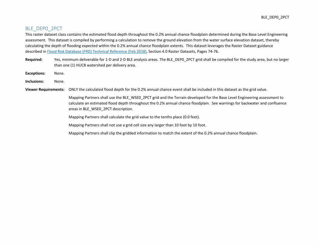
BLE_DEP0_2PCT
BLE_DEP0_2PCT This raster dataset class contains the estimated flood depth throughout the 0.2% annual chance floodplain determined during the Base Level Engineering
assessment. This dataset is compiled by performing a calculation to remove the ground elevation from the water surface elevation dataset, thereby
calculating the depth of flooding expected within the 0.2% annual chance floodplain extents. This dataset leverages the Raster Dataset guidance
described in Flood Risk Database (FRD) Technical Reference (Feb 2018), Section 4.0 Raster Datasets, Pages 74‐76.
Required: Yes, minimum deliverable for 1‐D and 2‐D BLE analysis areas. The BLE_DEP0_2PCT grid shall be compiled for the study area, but no larger
than one (1) HUC8 watershed per delivery area.
Exceptions: None.
Inclusions: None.
Viewer Requirements: ONLY the calculated flood depth for the 0.2% annual chance event shall be included in this dataset as the grid value.
Mapping Partners shall use the BLE_WSE0_2PCT grid and the Terrain developed for the Base Level Engineering assessment to
calculate an estimated flood depth throughout the 0.2% annual chance floodplain. See warnings for backwater and confluence
areas in BLE_WSE0_2PCT description.
Mapping Partners shall calculate the grid value to the tenths place (0.0 feet).
Mapping Partners shall not use a grid cell size any larger than 10 foot by 10 foot.
Mapping Partners shall clip the gridded information to match the extent of the 0.2% annual chance floodplain.

S_AOMI_PT
S_AOMI_PT This point feature class allows the Mapping Partner to identify and define areas within a BLE basins where additional technical information and or data
collection effort can refine the BLE results in a follow‐on study effort. The Mapping Partner shall include an entry in the S_AOMI_PT to communicate to
Federal, State and locals using the Base Level Engineering result where technical data (field survey or bridge structures) may further refine the flood
extents. This assists Discovery teams, local use and refinement and follow on technical teams to understand the opportunities to refine modeling where
the cursory engineering assessment identified additional information as beneficial for collection and data entry.
The intent of this coverage area is to allow a visualization and depiction of areas that may be refined in future local, state, regional or federal modeling
efforts. The items included in this file are intended to support local prioritization of study streams and identify for local communities where local
modeling efforts should be expended to build on the Base Level Engineering modeling, reducing local expenses and efforts to refine the base flood
elevation and flood extents within their communities.
This dataset leverages the previous Flood Risk database S_AOMI_PT feature class described in Flood Risk Database (FRD) Technical Reference (November
2016), Section 4.0 Raster Datasets, Pages 14‐16. Mapping Partners shall follow the instructions below for the compilation of this dataset elements
described within.
Required: Yes, minimum deliverable for 1‐D and 2‐D BLE analysis areas.
Exceptions: None.
Inclusions: At a minimum, Mapping Partners shall include a point at each structure that is expected to alter the analysis and assessment of flood risk
during the 1% annual chance event.
All inline structures (dams, weirs, and velocity dissipaters) should be included in the point file. Weir and velocity dissipater structures
that are significantly overtopped during the 1% annual chance event should include a note to indicate structure and inclusion may not
significantly affect the calculated water surface elevation for the 1% event.
Culverts should be included in the point file and include the information shown below. The location of hydraulic structures (inline
structures, dams, weirs, culverts, bridges, etc.) that ARE NOT included in the Base Level Engineering assessment or modeling
preparation. Points should be entered for structures that may refine the resultant flood extent shown in the current Base Level
Engineering assessment, for instance:
‐ Culvert groups and alignments, when added to the modeling may result in a lower upstream, larger downstream flood extent.
The entry of these culvert groups can also leverage HEC‐RAS calculations for head loss through the structure.
‐ Mapping Partners should identify the need for as‐built road crossing and/or field survey/measurements in the surround of the
structure – identifying modeling refinement opportunities to refine the modeling output (calculated water surface elevation and
flood extent) in the immediate vicinity of a culvert/bridge/utility crossing that is not detailed in the Base Level Engineering
model geometry.
‐ Also indicate that the hydrology should be reviewed for a flow change location based on development of rating curve for the
structure in this area.

S_AOMI_PT
LiDAR processing may not remove all vegetation from the bare earth terrain that the Base Level Engineering models are built from.
‐ Mapping Partners shall include an entry in the S_AOMI _PT or S_AOMI_AR file to depict the location of LiDAR processing areas
that should be supplemented with field survey information if a reach is identified for further study.
‐ Including the point or area within the S_AOMI_PT/AR file will identify areas where field survey is needed to validate the ground
information that was used in Base Level Engineering efforts.
Bridges should be included in the point file. Bridges that are significantly above the calculated 1% annual chance water surface elevation
should include a note indicating that the low chord of the bridge is significantly above the 1% WSEL and may require assessment in
extreme events only, may not significantly affect the 1% WSEL analysis.
‐ Mapping Partners shall use care and NOT include points for bridge structures that are significantly elevated from the Base Flood.
Some large streams are crossed by significantly elevated road and railway crossings, while there are several piers, the structure
low chord is significantly elevated above the calculated water surface elevation for the 0.2% annual chance event.
‐ Detailed models and field survey may be included in modeling in the future but end users should be alerted that minimal
refinement of the flood extent is expected by updates to structures of this sort.
‐ If the Mapping Partner includes a structure of this nature, the comments should indicate minimal flood extent refinement is
expected with detailed modeling near the identified structure.
Low water crossings and utility crossings that will be several feet under water during the 1% annual chance event may be included but
should also include a note that the structure is not expected to significantly affect the 1% annual chance event analysis if surveyed or
included in a future analysis. May indicate that only detailed and floodway analysis may want to include these structures.
Pedestrian bridges that are expected to be significantly overtopped should be indicated as such, Mapping Partners shall indicate that
inclusion of small bridges and significantly overtopped structures may not create a significant change in the 1% and 0.2% water surface
elevations and or flood extent.
Optional items include:
Location of repetitive loss properties (generalize) – Indicators of repeated flood‐related insurance claims. Care must be taken to no
identify claim or property specific losses and must abide privacy requirements.
At‐Risk Essential Facilities – Essential/critical facilities that could cause significant problems to individuals/communities during their
response during or recovery post‐flood. These include, but are not limited to, hospitals, schools, water/wastewater treatment facilities,
police stations, etc.
Viewer Requirements: None.
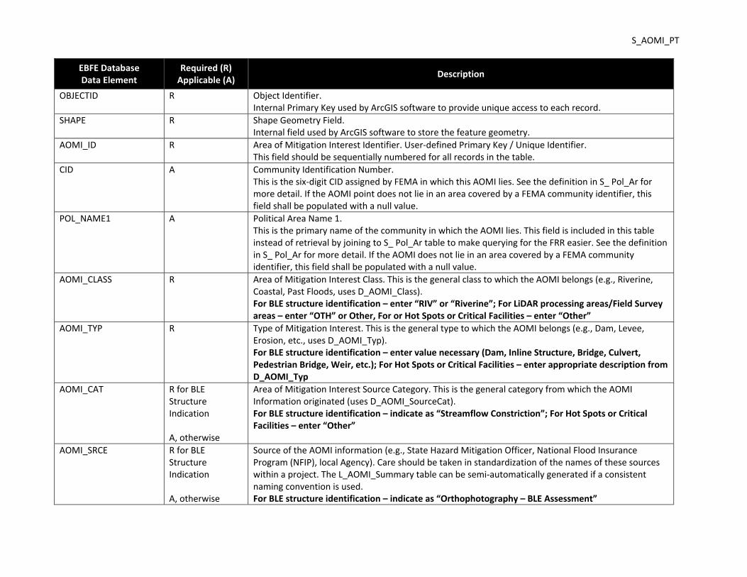
S_AOMI_PT
EBFE Database Data Element
Required (R) Applicable (A)
Description
OBJECTID R Object Identifier. Internal Primary Key used by ArcGIS software to provide unique access to each record.
SHAPE R Shape Geometry Field. Internal field used by ArcGIS software to store the feature geometry.
AOMI_ID R Area of Mitigation Interest Identifier. User‐defined Primary Key / Unique Identifier. This field should be sequentially numbered for all records in the table.
CID A Community Identification Number. This is the six‐digit CID assigned by FEMA in which this AOMI lies. See the definition in S_ Pol_Ar for more detail. If the AOMI point does not lie in an area covered by a FEMA community identifier, this field shall be populated with a null value.
POL_NAME1 A Political Area Name 1. This is the primary name of the community in which the AOMI lies. This field is included in this table instead of retrieval by joining to S_ Pol_Ar table to make querying for the FRR easier. See the definition in S_ Pol_Ar for more detail. If the AOMI does not lie in an area covered by a FEMA community identifier, this field shall be populated with a null value.
AOMI_CLASS R Area of Mitigation Interest Class. This is the general class to which the AOMI belongs (e.g., Riverine, Coastal, Past Floods, uses D_AOMI_Class). For BLE structure identification – enter “RIV” or “Riverine”; For LiDAR processing areas/Field Survey areas – enter “OTH” or Other, For or Hot Spots or Critical Facilities – enter “Other”
AOMI_TYP R Type of Mitigation Interest. This is the general type to which the AOMI belongs (e.g., Dam, Levee, Erosion, etc., uses D_AOMI_Typ). For BLE structure identification – enter value necessary (Dam, Inline Structure, Bridge, Culvert, Pedestrian Bridge, Weir, etc.); For Hot Spots or Critical Facilities – enter appropriate description from D_AOMI_Typ
AOMI_CAT R for BLE Structure Indication A, otherwise
Area of Mitigation Interest Source Category. This is the general category from which the AOMI Information originated (uses D_AOMI_SourceCat). For BLE structure identification – indicate as “Streamflow Constriction”; For Hot Spots or Critical Facilities – enter “Other”
AOMI_SRCE R for BLE Structure Indication A, otherwise
Source of the AOMI information (e.g., State Hazard Mitigation Officer, National Flood Insurance Program (NFIP), local Agency). Care should be taken in standardization of the names of these sources within a project. The L_AOMI_Summary table can be semi‐automatically generated if a consistent naming convention is used. For BLE structure identification – indicate as “Orthophotography – BLE Assessment”

S_AOMI_PT
EBFE Database Data Element
Required (R) Applicable (A)
Description
AOMI_INFO R for BLE Structure Indication A, otherwise
AOMI Information. This field provides the specific reasons this location is considered an AOMI. For BLE structure identification – indicate one of the following items
‐ Road Name or Structure Name ‐ Approximate Location
For Critical Facility identification – indicate type of facility (hospital, school, fire station, etc.)
NOTES R for BLE Structure Indication A, otherwise
Comments explaining the relevance of this AOMI point. The size of this field provides the user space to supply more detail in a free form format regarding the relevance of this AOMI. For BLE structure identification – indicate one of the following items
‐ Potential structure overtopping ‐ Survey/As‐Built for structure info may support additional modeling refinement ‐ Dam operational info will support additional H&H model refinement ‐ Weir/Low Water Crossing/Pedestrian Bridge location. May refine lower event analysis,
expected to be significantly overtopped during the 1% event ‐ Bridge significantly higher than 1% WSEL, may include in extreme event analysis
Bridge abutments/piers may significantly impact 1% H&H modeling
HUC8_CODE R WBD 8‐digit Hydrologic Unit Code for the sub‐basin in which the AOMI point lies.
CASE_NO R FEMA Case Number. See the CASE_NO field in the S_FRD_Proj_Ar feature class for a more detailed description.
VERSION_ID R Version Identifier. Identifies the product version and relates the feature to standards according to which it was created.
SOURCE_CIT R Source Citation from L_SOURCE_CIT. See field definition in L_Source_Cit for more detail.

S_AOMI_AR
S_AOMI_AR This polygon feature class depicts the areas that warrant further investigation or research for possible mitigation (significant land use change, non‐levee
embankments, coastal features, mitigation successes, key emergency routes, etc.). The intent of this coverage area is to allow a visualization and
depiction of areas that may be refined in future local, state, regional or federal modeling efforts.
This dataset leverages the Flood Risk Database S_AOMI_Ar feature class described in Flood Risk Database (FRD) Technical Reference (Feb 2018),
Section 3.0 Tables and Feature Classes, Pages 9‐10. Mapping Partners shall follow the instructions within the Technical Reference for the compilation of
this dataset elements described within.
Required: No. Optional layer that can be used to identify mitigation areas including significant land use changes, future mitigation actions,
mitigation successes, etc.
Exceptions: None.
Inclusions: Possible inclusions include:
Significant land use change – Proposed/recent development and areas with current or project population growth. Potential sources for
this data include: Discovery meeting materials and discussions; community comprehensive plans; state growth management plans and
real estate trends. If review of an aerial image identifies centralized development in a location that soils, or land use information define
as natural/non‐impervious, the Mapping Partner shall include a polygon to describe a future prioritization area for local refinement and
identify that the hydrology may require additional review. If intense and centralized development significantly alters the percent of
impervious land in a watershed or sub‐basin within the engineering analysis, the flow volume may be altered.
Altered stream/drainage channel location ‐ If local development has modified a stream channel location/alignment Mapping Partners
shall include a polygon to describe the general area of disagreement between the LiDAR/engineering modeling and a recent aerial.
Coastal structures – Structures along the coast that “harden” the shoreline, interrupt the natural dynamic shoreline process or
accelerate erosion along the shore. Potential sources for this data include: Discovery meeting materials and discussions; community
input; NOAA National Shoreline Survey; State Coastal Zone Management programs and Beach Management Plans.
Mitigation successes – Structural/grading projects that mitigate flooding. These can include but are not limited to increase in size of
storm drain pipe, drainage rerouted via grading, floodwall construction, etc.
Key emergency routes overtopped – Key emergency and evacuation routes that are overtopped during the 4‐percent or more annual
chance event. Potential sources for this data include: Discovery meeting materials and discussions; community stakeholders and flood
profiles.
Non‐levee embankments – Embankments/structures that are not designed for flood control but have an impact on flooding. These may
include but are not limited to railroad embankments and roadways.

S_AOMI_AR
Non‐accredited levees – Levees that do not meet the 44 CFR Part 65.10 or those that have recently had their provisionally accredited
status expire. Potential sources for this data include: Discovery meeting materials and discussions; community input; and National Levee
Database.
Storage Areas Modeled – Numerous stock tanks, local dams/reservoirs, and other detention structures exist throughout the Region,
these structures may alter the nature of flow and timing within a riverine environment. The Mapping Partner shall include polygons to
describe modeled Storage Areas utilized in the Base Level Engineering HEC‐HMS and HEC‐RAS efforts. Inclusion of these items allows the
Mapping Partner to communicate that there is opportunity for refinement of the hydrology and expansion of the hydraulic modeling
prepared in the Base Level Engineering effort.
Optional items include:
Past claims hot spots – Indicators of repeated flood‐related insurance claims. Care must be taken to no identify claim or property specific
losses and must abide privacy requirements.
Viewer Requirements: None.
EBFE Database Data Element
Required (R) Applicable (A)
Description
OBJECTID R Object Identifier. Internal Primary Key used by ArcGIS software to provide unique access to each record.
SHAPE R Shape Geometry Field. Internal field used by ArcGIS software to store the feature geometry.
AOMI_ID R Area of Mitigation Interest Identifier. User‐defined Primary Key / Unique Identifier. This field should be sequentially numbered for all records in the table.
CID A Community Identification Number. This is the six‐digit CID assigned by FEMA in which this AOMI lies. See the definition in S_Pol_Ar for more detail. If the AOMI does not lie in an area covered by a FEMA community identifier, this field shall be populated with a null value.
POL_NAME1 A Political Area Name 1. This is the primary name of the community in which the AOMI lies. This field is included in this table instead of retrieval by joining to S_Pol_Ar table. See the definition in S_Pol_Ar for more detail. If the AOMI does not lie in an area covered by a FEMA community identifier, this field shall be populated with a null value.
AOMI_CLASS R Area of Mitigation Interest Class. This is the general class to which the AOMI belongs (e.g., Riverine, Coastal, other, uses D_AOMI_Class). For BLE – enter “Riverine or Coastal”, whichever is applicable
AOMI_TYP R Type of Mitigation Interest. This is the general type to which the AOMI belongs (e.g., Dam, Levee,

S_AOMI_AR
EBFE Database Data Element
Required (R) Applicable (A)
Description
Erosion, etc., uses D_AOMI_Typ). For BLE – enter value necessary (Significant land use change, mitigation success, etc.)
AOMI_INFO A AOMI Information. This field provides the specific reasons this location is considered an AOMI. Comments explaining the relevance of this AOMI point.
HUC8_CODE R WBD 8‐digit Hydrologic Unit Code for the sub‐basin in which the AoMI lies.
CASE_NO R FEMA Case Number. See the CASE_NO field in the S_FRD_Proj_Ar feature class for a more detailed description.
VERSION_ID R Version Identifier. Identifies the product version and relates the feature to standards according to which it was created.
SOURCE_CIT R Source Citation from L_SOURCE_CIT. See field definition in L_Source_Cit for more detail.
Mapping Partners may add information collected at Discovery, to include, but not limited to: areas of mitigation success, significant land use changes,
areas of local community interest for future mitigation action, indication of major flood sources for communities, coastal features, non‐ accredited levees,
etc.

S_FRAC_AR
S_FRAC_AR This polygon feature class is the spatial foundation for all census block‐based flood risk assessment data. All the inventory and damage estimates for flood
risk assessments are stored and performed at the Census Block level This feature class contains the spatial location of the Census Blocks for the project.
The census block geometries shall be based on the version of Hazus used to perform the analysis, which should be documented in the metadata.
This should include information on whether the census block type was homogenous or dasymetric (see Flood Risk Assessment Guidance for more
information). This feature class also stores the Asset Replacement Value, as well as the estimated flood risk assessment results for each block. This
feature class is required to be populated when the Flood Risk Assessment dataset is produced.
This dataset leverages the Flood Risk Database S_FRAC_Ar feature class described in Flood Risk Database (FRD) Technical Reference (Feb 2018),
Section 3.0 Tables and Feature Classes, Pages 22‐25. Mapping Partners shall follow the instructions within the Technical Reference for the compilation of
this dataset elements described within.
Note (April 2019): The S_FRAC_AR dataset replaces the historic submittal of the S_CenBlk_AR dataset and L_RA_Results table within the Spatial
deliverables for each BLE submittal.
Required: Yes, minimum deliverable for 1‐D and 2‐D BLE analysis areas.
Exceptions: None.
Inclusions: Hazus results based on WSEL and Depth of flooding grids produced in Base Level Engineering effort.
Viewer Requirements: None.
EBFE Database Data Element
Required (R) Applicable (A)
Description
OBJECTID R Object Identifier. Internal Primary Key used by ArcGIS software to provide unique access to each record.
SHAPE R Shape Geometry Field. Internal field used by ArcGIS software to store the feature geometry.
CEN_BLK_ID R This field should be populated with the Census Block identifier. This identifier is based on the following format with an optional single alphabetic character suffix to accommodate the 2010 decennial Census:
06 071 003602 1003 State County Census Census Block Group Tract Block Group
ARV_BG_TOT REQUIRED for BLE Asset Replacement Value of Buildings of All Structure Types. Obtained from General Building Stock data, in whole dollars.
ARV_CN_TOT REQUIRED for BLE Asset Replacement Value of Contents for All Structure Types. Obtained from General Building Stock data, in whole dollars.

S_FRAC_AR
EBFE Database Data Element
Required (R) Applicable (A)
Description
TOT_LOSS01 REQUIRED for BLE 1 Percent Chance Total Losses. For each Census Block, the estimate of the total value of all losses for the return period.
BL_TOT01 REQUIRED for BLE 1 Percent Chance Total Building Losses. For each Census Block, the estimate of the total value of building losses for the return period.
CL_TOT01 REQUIRED for BLE 1 Percent Chance Total Building Losses. For each Census Block, the estimate of the total value of content losses for the return period.
HIDE HAZARD_TYP Hazard Type. Indicates the Hazard Type for which the loss fields apply. This field uses D_Hazard_Type.
HIDE SCENAR_ID Levee or Dam Scenario Identification.
HIDE TOT_LOSS10 10 Percent Chance Total Losses. For each Census Block, the estimate of the total value of all losses for the return period.
HIDE BL_TOT10 10 Percent Chance Total Building Losses. For each Census Block, the estimate of the total value of building losses for the return period.
HIDE CL_TOT10 10 Percent Chance Total Building Losses. For each Census Block, the estimate of the total value of content losses for the return period.
HIDE TOT_LOSS04 4 Percent Chance Total Losses. For each Census Block, the estimate of the total value of all losses for the return period.
HIDE BL_TOT04 4 Percent Chance Total Building Losses. For each Census Block, the estimate of the total value of building losses for the return period.
HIDE CL_TOT04 4 Percent Chance Total Building Losses. For each Census Block, the estimate of the total value of content losses for the return period.
HIDE TOT_LOSS02 2 Percent Chance Total Losses. For each Census Block, the estimate of the total value of all losses for the return period.
HIDE BL_TOT02 2 Percent Chance Total Building Losses. For each Census Block, the estimate of the total value of building losses for the return period.
HIDE CL_TOT02 2 Percent Chance Total Building Losses. For each Census Block, the estimate of the total value of content losses for the return period.
HIDE TOT_LSS0_2 0.2 Percent Chance Total Losses. For each Census Block, the estimate of the total value of all losses for the return period.
HIDE BL_TOT0_2 0.2 Percent Chance Total Building Losses. For each Census Block, the estimate of the total value of building losses for the return period.
HIDE CL_TOT0_2 0.2 Percent Chance Total Building Losses. For each Census Block, the estimate of the total value of content losses for the return period.
HIDE TOT_LSSAAL Average Annualized Total Losses. For each Census Block, the estimate of the total value of all losses for the return period.

S_FRAC_AR
EBFE Database Data Element
Required (R) Applicable (A)
Description
HIDE BL_TOTAAL Average Annualized Total Building Losses. For each Census Block, the estimate of the total value of building losses for the return period.
HIDE CL_TOTAAL Average Annualized Total Building Losses. For each Census Block, the estimate of the total value of content losses for the return period.
HUC8_CODE R WBD 8‐digit Hydrologic Unit Code for the sub‐basin in which the Census Block lies. If a Census Block crosses a HUC‐8 boundary, the field shall be populated with the HUC‐8 value in which the majority of the Census Block lies.
CASE_NO R FEMA Case Number. See the CASE_NO field in S_FRD_Proj_Ar for more detail.
VERSION_ID R Version Identifier. Identifies the product version and relates the feature to standards according to which it was created.
SOURCE_CIT R Source Citation from L_SOURCE_CIT. See field definition in L_Source_Cit for more detail.
SHAPE_LENGTH R Internal field used by ArcGIS software to store the length of the feature’s geometry.
SHAPE_AREA R Internal field used by ArcGIS
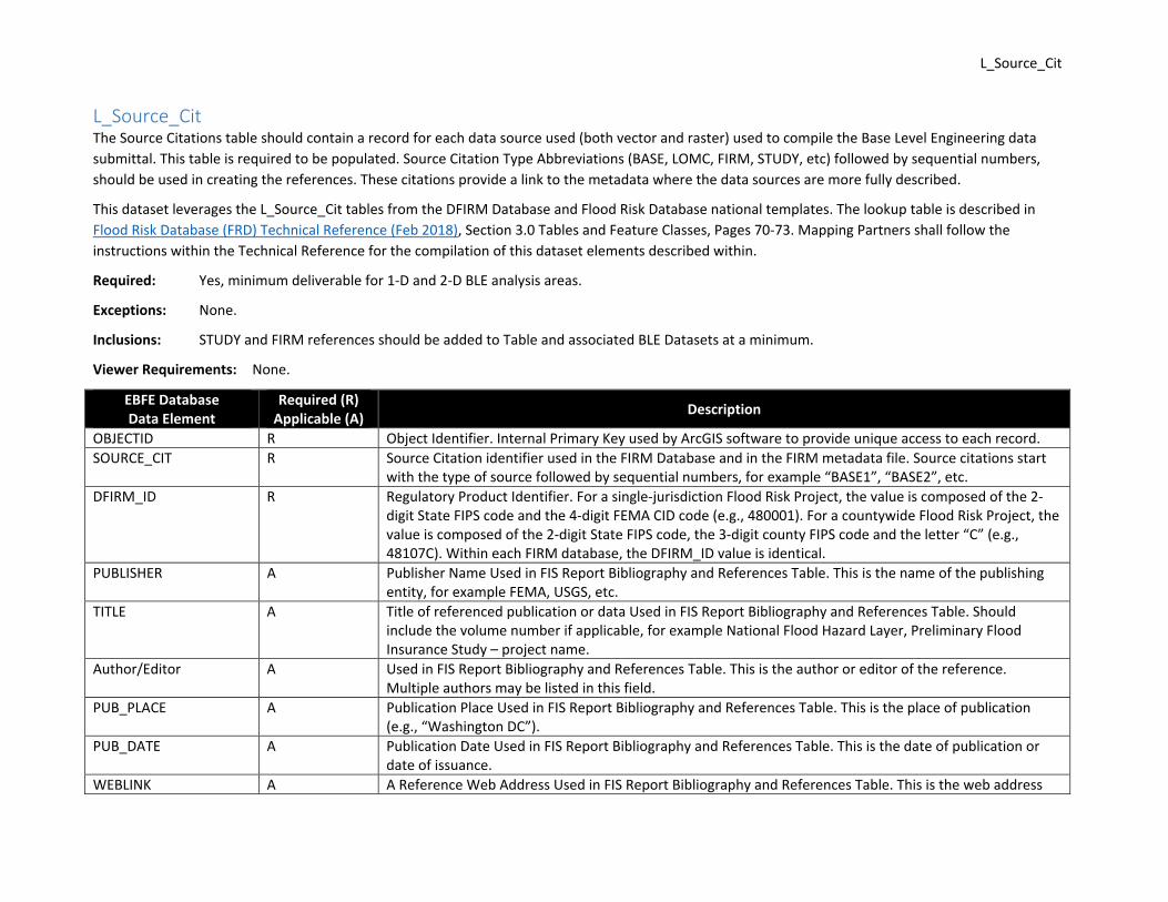
L_Source_Cit
L_Source_Cit The Source Citations table should contain a record for each data source used (both vector and raster) used to compile the Base Level Engineering data
submittal. This table is required to be populated. Source Citation Type Abbreviations (BASE, LOMC, FIRM, STUDY, etc) followed by sequential numbers,
should be used in creating the references. These citations provide a link to the metadata where the data sources are more fully described.
This dataset leverages the L_Source_Cit tables from the DFIRM Database and Flood Risk Database national templates. The lookup table is described in
Flood Risk Database (FRD) Technical Reference (Feb 2018), Section 3.0 Tables and Feature Classes, Pages 70‐73. Mapping Partners shall follow the
instructions within the Technical Reference for the compilation of this dataset elements described within.
Required: Yes, minimum deliverable for 1‐D and 2‐D BLE analysis areas.
Exceptions: None.
Inclusions: STUDY and FIRM references should be added to Table and associated BLE Datasets at a minimum.
Viewer Requirements: None.
EBFE Database Data Element
Required (R) Applicable (A)
Description
OBJECTID R Object Identifier. Internal Primary Key used by ArcGIS software to provide unique access to each record.
SOURCE_CIT R Source Citation identifier used in the FIRM Database and in the FIRM metadata file. Source citations start with the type of source followed by sequential numbers, for example “BASE1”, “BASE2”, etc.
DFIRM_ID R Regulatory Product Identifier. For a single‐jurisdiction Flood Risk Project, the value is composed of the 2‐digit State FIPS code and the 4‐digit FEMA CID code (e.g., 480001). For a countywide Flood Risk Project, the value is composed of the 2‐digit State FIPS code, the 3‐digit county FIPS code and the letter “C” (e.g., 48107C). Within each FIRM database, the DFIRM_ID value is identical.
PUBLISHER A Publisher Name Used in FIS Report Bibliography and References Table. This is the name of the publishing entity, for example FEMA, USGS, etc.
TITLE A Title of referenced publication or data Used in FIS Report Bibliography and References Table. Should include the volume number if applicable, for example National Flood Hazard Layer, Preliminary Flood Insurance Study – project name.
Author/Editor A Used in FIS Report Bibliography and References Table. This is the author or editor of the reference. Multiple authors may be listed in this field.
PUB_PLACE A Publication Place Used in FIS Report Bibliography and References Table. This is the place of publication (e.g., “Washington DC”).
PUB_DATE A Publication Date Used in FIS Report Bibliography and References Table. This is the date of publication or date of issuance.
WEBLINK A A Reference Web Address Used in FIS Report Bibliography and References Table. This is the web address

L_Source_Cit
for the reference, if applicable.
MEDIA A Media through which the source data were received.
CASE_NO R FEMA Case Number. See the CASE_NO field in S_FRD_Proj_Ar for more detail.
VERSION_ID R Version Identifier. Identifies the product version and relates the feature to standards according to which it was created.

CNMS Datasets
CNMS Database For BLE projects, there are two touchpoints when CNMS must be updated; once at scoping (within 30 days of the project start) and again once
engineering on the BLE study is completed (Production Phase Update). FEMA’s CNMS Technical Reference should be referenced during completion of
these tasks. Mapping Partners shall request the latest version of the CNMS Database from the RSC for the project area prior to completing each of these
touchpoints.
BLE Scoping Phase Update
FEMA requires that only BLE studies that are used to update the regulatory FIRM and counted in the Risk MAP Project Planning and Purchasing Portal (P4)
as initiated miles will be treated as initiated miles in CNMS and receive the BEING STUDIED classification. Fully automated LSAE or BLE studies not being
used to update the regulatory FIRM can be leveraged for assessment work only and may have tracking fields in CNMS populated but will not receive a
BEING STUDIED classification and will not count toward NVUE initiated. The Mapping Partner will consult with the RSC or FEMA Region to confirm
whether the BLE study is being used to update the regulatory FIRM and counted in P4 as initiated miles. Some Regional Guidance has been previously
prepared to detail the Roles and Responsibilities of provider teams and Mapping Partners that may be of assistance (available at RMD SharePoint > R6 >
Resources > Regional Delivery Guidance:
CNMS Roles & Responsibilities – Flood Risk Studies
CNMS Roles & Responsibilities – Quarterly Regional Database Maintenance
CNMS Guidance – Unmapped Unstudied Streams
Required: Yes, minimum deliverable for 1‐D and 2‐D BLE analysis areas.
Exceptions: None.
Inclusions: None.
Viewer Requirements: None.
1. Add Unmapped Miles into S_Studies_Ln:
BLE studies often extend past the reaches representing effective SFHA in the CNMS inventory, since unmapped stream reaches are
gathered for drainage areas > 0.5 sq. mile in urban areas and > 1.0 sq. mile in rural areas. Where BLE analysis does not overlap with
existing CNMS inventory (i.e. in non‐SFHA areas), these unmapped stream reaches should be loaded into S_Studies_Ln and edited to tie
into existing features. The most common source for unmapped stream features will be the S_Unmapped_Ln feature class in CNMS; staff
should first contact the Compass RSC CNMS lead to confirm the appropriate source to use. If unmapped miles are not available at the
time of scoping, they can be added later to the BLE study area during the Production Phase Update.

CNMS Datasets
Once new stream centerline features representing unmapped miles have been added to S_Studies_Ln, the following basic fields will need
to be populated:
REACH_ID: see Table F‐1 in CNMS Technical Reference, February 2018
STUDY_ID: see Table F‐1 in CNMS Technical Reference, February 2018
COFIPS: see Table F‐1 in CNMS Technical Reference, February 2018
CID: see Table F‐1 in CNMS Technical Reference, February 2018
WTR_NM: see Table F‐1 in CNMS Technical Reference, February 2018; BLE study is typically the best source of these water names
FLD_ZONE: effective flood zone (“X” for unmapped miles)
VALIDATION_STATUS: for all unmapped miles, “ASSESSED”
MILES: see Table F‐1 in CNMS Technical Reference, February 2018
SOURCE: see Table F‐1 in CNMS Technical Reference, February 2018 (“COUNTY DFIRM DATABASE ACQUIRED DURING STUDY
PERIOD” is an acceptable default entry for BLE unmapped miles)
REASON: note the BLE project name and BS_MIP_CASE_NUMBER, if available (see Step 3 “BEING STUDIED Fields” below)
HUC8_KEY: see Table F‐1 in CNMS Technical Reference, February 2018
STUDY_TYPE: description of effective study type (for Zone X, “UNMAPPED d”)
TIER: “TIER 0” (classification for Zone X (non‐SFHA))
LINE_TYPE: e.g. “RIVERINE”; see Table F‐1 in CNMS Technical Reference, February 2018
FBS_CMPLNT: “Unknown” (default entry for Zone X)
FBS_CHKDT: current date (default entry for Zone X)
FBS_CTYP: “COUNTY ‐ BULK ATTRIBUTION” (default entry for Zone X)
DUPLICATE: see Table F‐1 in CNMS Technical Reference, February 2018 (Zone X is “CATEGORY 3” by default)
In addition, all of the fields detailed in Step 2 “BLE Tracking Fields” and Step 3 “BEING STUDIED Fields” below will need to be populated,
with the following exception:
BS_STDYTP: description of new study type (“NEW APPROXIMATE” for effective Zone X)
2. BLE Tracking Fields:
The following fields in S_Studies_Ln should be populated for all reaches within the BLE project footprint (Zone A, Detailed, and Unmapped
reaches), as this information can facilitate the query of BLE extent in CNMS:
BLE: BLE study classification (select either Tier A, B, C, D, E; 2D; or LSAE; see Table 1 of the BLE Analysis and Mapping Guidance,
February 2018 for domain code descriptions. Most Compass BLE studies are either Tier A or B. If unsure, default is Tier A.)

CNMS Datasets
BLE_POC: Preferred FEMA Regional contact or project manager to be added to the Point_of_Contact Table. Instructions for
creating this 12‐digit number can be found in Table F‐6 of the CNMS Technical Reference, February 2018 (e.g. “482450500001”;
the first five digits are the county, “05” is the identifier for the POC table, and the last five digits are a counter for each unique POC
entry for that county)
BLE_DATE: date that engineering was completed on the BLE study
3. BEING STUDIED Fields:
All the approximate reaches included in the BLE study are classified with a Status Type of “Being Studied.” This update in Status Type
requires additional fields specific to the BLE study to be populated at this point as well. The definition query created for S_Studies_Ln
should be updated to isolate only the Zone A reaches located within the BLE study area (i.e. CO_FIPS = '48141' AND FLD_ZONE = 'A' or
HUC8_KEY = '12030102' AND FLD_ZONE = 'A'). The following fields in S_Studies_Ln should then be populated as follows:
STATUS_TYPE: “BEING STUDIED”
STATUS_DATE: current date
DATE_RQST: current date
BS_MIP_CASE_NUMBER: FEMA‐assigned case number used for storage on the Mapping Information Platform (MIP)
BS_ZONE: flood zone of the new study (“A” for BLE studies”)
BS_STDYTYP: description of new study type (“UPDATED APPROXIMATE” for existing Zone A)
BS_HYDRO_M: hydrologic method/model used in BLE study (e.g. “REGRESSION EQUATIONS”)
BS_HYDRO_CMT: comment field regarding hydrologic method/model
BS_HYDRA_M: hydraulic method/model used in BLE study (e.g. “HEC‐RAS 4.1”)
BS_HYDRA_CMT: comment field regarding hydraulic method/model
BS_FY_FUND: fiscal year from which BLE study is funded
PRELIM_DATE: date the BLE study will go preliminary (This date is not known at this time, so it should be populated with a date
far in the future, such as 1/1/2030. This field will get updated again when a preliminary date is known.)
LFD_DATE: date the letter of final determination for the BLE study is issued (This date is not known at this time, so it should be
populated with a date one year ahead of the PRELIM_DATE entered, such as 1/1/2031. This field will get updated again when the
LFD is issued.)
Much of the information needed to complete these fields can be collected from the BLE Project Manager or Technical Lead. Prior to
completing the attribution of these fields, best practice is to perform a QC check on the HUC8 attribution of all reaches located in the

CNMS Datasets
study area to be sure it is correct and that reaches are split at the HUC boundary. This QC should occur before the definition query is
created for the BLE project footprint.
4. Run the CNMS QC tool:
As with all CNMS submittals, the Mapping Partner will run the CNMS QC Tool on their updated CNMS database extract and address all
Critical and Secondary errors prior to delivery of the CNMS database. The CNMS QC Tool is typically updated once a year when an
updated CNMS Schema is distributed. If necessary, the Mapping Partner can obtain the latest copy of the QC Tool from the RSC.
BLE Production Phase Update
The BLE Production Phase Update to the CNMS DB is focused on the population of the A1‐A4 and A5 Validation Assessment Checks and the
resulting update to the Validation Status classification. Fields populated during the Scoping Phase Update should first be reviewed for accuracy and
updated with newly provided information as necessary (for example, a BLE analysis completion date). Unmapped miles can be added at this point
if not previously, see Step 1 “Add Unmapped Miles into S_Studies_Ln” above.
Required: Yes, minimum deliverable for 1‐D and 2‐D BLE analysis areas.
Exceptions: None.
Inclusions: CNMS database with the revised S_Studies_Ln feature and the validation points (as a separate shapefile) should be submitted
along with the associated BLE report documenting the results.
Viewer Requirements: None.
For the following steps, a definition query should be created for S_Studies_Ln isolating the approximate reaches located within the BLE study area
(i.e. CO_FIPS = '48141' AND FLD_ZONE = 'A' or HUC8_KEY = '12030102' AND FLD_ZONE = 'A').
1. A1 – A4 Assessment Existing Zone A studies within the BLE study area must go through the entire Zone A validation assessment process. Several sources of data are
needed to complete this step:
Effective FIS report
Effective DFIRM DB
LOMR data (if applicable)
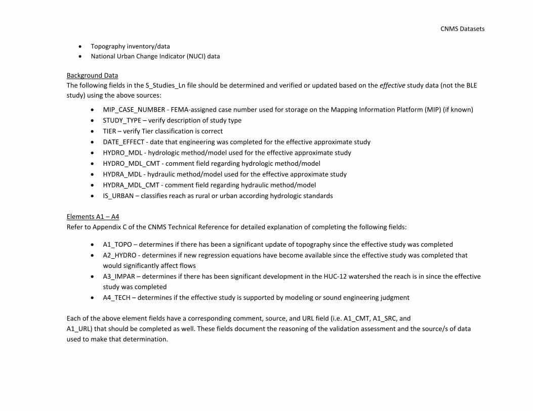
CNMS Datasets
Topography inventory/data
National Urban Change Indicator (NUCI) data
Background Data The following fields in the S_Studies_Ln file should be determined and verified or updated based on the effective study data (not the BLE
study) using the above sources:
MIP_CASE_NUMBER ‐ FEMA‐assigned case number used for storage on the Mapping Information Platform (MIP) (if known)
STUDY_TYPE – verify description of study type
TIER – verify Tier classification is correct
DATE_EFFECT ‐ date that engineering was completed for the effective approximate study
HYDRO_MDL ‐ hydrologic method/model used for the effective approximate study
HYDRO_MDL_CMT ‐ comment field regarding hydrologic method/model
HYDRA_MDL ‐ hydraulic method/model used for the effective approximate study
HYDRA_MDL_CMT ‐ comment field regarding hydraulic method/model
IS_URBAN – classifies reach as rural or urban according hydrologic standards
Elements A1 – A4
Refer to Appendix C of the CNMS Technical Reference for detailed explanation of completing the following fields:
A1_TOPO – determines if there has been a significant update of topography since the effective study was completed
A2_HYDRO ‐ determines if new regression equations have become available since the effective study was completed that
would significantly affect flows
A3_IMPAR – determines if there has been significant development in the HUC‐12 watershed the reach is in since the effective
study was completed
A4_TECH – determines if the effective study is supported by modeling or sound engineering judgment
Each of the above element fields have a corresponding comment, source, and URL field (i.e. A1_CMT, A1_SRC, and
A1_URL) that should be completed as well. These fields document the reasoning of the validation assessment and the source/s of data
used to make that determination.

CNMS Datasets
2. A5 Assessment
The A5 check involves a comparison of the refined Zone engineering analysis (BLE study) and the effective Zone A study. The process results in pass/fail
classified points across the full study area. Even though all checks A1‐A5 will be completed, only the result of the A5 check will be used to classify the
effective Zone A as either Valid or Unverified. The A5 assessment procedures in appendix C of the CNMS Technical reference are primarily geared toward
1D BLE studies. When a BLE study is performed using 2‐D methods, the steps for conducting the A5 validation requires some modification. See the
accompanying (Appendix A) for specific instructions on how the A5 check should be performed when using 2‐D BLE outputs.
Before reclassifying the validation status of the effective Zone As within the BLE project footprint, the Mapping Partner will consult with the RSC to
determine if any effective Zone A studies classified as VALID in the project area should be subject to the A5 assessment results. For example, any recently
incorporated LOMRs or other valid Zone A studies with a recent STATUS_DATE should be reviewed prior to changing to UNVERIFIED.
Note that any effective detailed studies (e.g., Zone AE, AO, AH, AR) within the BLE project footprint will not be subject to assessment checks A1‐A5 and
will not have their validation status changed. Validation assessment of any effective detailed studies, which have a unique set of checks described in the
CNMS Tech Ref, will not be part of the BLE submittal unless explicitly directed by the Region.
Mapping partners need to pay special attention to attribute updates if there are any ongoing studies (PMR for example) within the BLE project footprint.
For records with this situation (STATUS_TYPE field in CNMS is currently set to BEING STUDIED), steps 1‐3 below can still proceed, but for step 4 only the
STATUS_DATE and DATE_RQST fields should be updated. No other fields will be updated (BS fields).
3. Run the CNMS QC tool
As with all CNMS submittals, the Mapping Partner will run the CNMS QC Tool on their updated CNMS database extract and address all Critical and
Secondary errors prior to delivery of the CNMS database. The CNMS QC Tool is typically updated once a year when an updated CNMS Schema is
distributed. If necessary, the Mapping Partner can obtain the latest copy of the QC Tool from the RSC.
4. CNMS Submittal and Reporting
The updated CNMS database with the revised S_Studies_Ln feature and the validation points (as a separate shapefile) should be submitted along with the
associated BLE report documenting the results.

CNMS Datasets
5. CNMS Results Graphic and Table (REQUIRED) – BLE Submittal Report
Mapping Partners should include a graphic representation of the CNMS validation results in their Base Level Engineering report. Mainly, this allows the
FEMA Project Monitor and any community end user to understand the location of streams determined to be valid through the CNMS validation process,
it also indicates areas where the Base Level Engineering assessment identified issues with the current flood hazard inventory. One example of CNMS
results visualization is included in Figure
11 for reference.
Mapping Partners may review the results
and determine different visualization
schemas and components.
The Region’s investment in Base Level
Engineering data also allows assessment
of the current inventory of streams and
stream validation status throughout each
of the Base Level Engineering basins.
Mapping Partners shall include a table of
pre‐ and post‐Base Level Engineering
stream validation status. The BLE Report
template (V2) has been updated (April
2019) to include a table for Mapping
Partners to communicate the number of
stream miles in each HUC8 (County or
River Basin) that are determined to be
valid by data created in the Base Level
Engineering assessment.
Figure 11: CNMS Validation Graphic (HUC8 Study Area)

Hazus Datasets
HAZUS DATASETS To populate the S_FRAC_Ar dataset, an Advanced Hazus analysis will need to be performed for each BLE project area. For the advanced analysis, the
flooding extent is represented in the various flood depth grids prepared during the Base Level Engineering assessment (these grids may also be referred
to as ‘refined’ grids) that the user will need to import into Hazus. Once the Base Level Engineering Flood Depth Grids are imported, Hazus will calculate
the losses. Once the losses are produced, those values will be used to populate the attributes required within S_FRAC_Ar. When loading the data into
the dataset, the user will need to multiply the loss fields by 1,000 to reflect actual dollars.
Required: Yes, minimum deliverable for 1‐D and 2‐D BLE analysis areas.
Exceptions: None.
Inclusions: None.
Viewer Requirements: None.
To populate the S_FRAC_Ar dataset, the user will need to complete the advanced Hazus analysis, and export the following features will be exported
from the Hazus loss menu:
o Residential_Total
o Commercial_Total
o Total
For specific information regarding how to process a basic and/or advanced Hazus analysis please refer to the current available Hazus User Manuals
and Technical Reference Materials available in the FEMA Library.
Once the losses have been populated in the S_FRAC_Ar dataset located within the BLE Database, the user will need to export out the Hazus project. The
exported Hazus project is referred to as an .hpr. For instructions to export a Hazus project, please refer to the current Hazus User Manual.
As a reminder, the losses are reported via census blocks. It is important to note that Hazus version 3.2 and current use dasymetric census blocks.
Dasymetric mapping removes undeveloped areas (such as areas covered by other bodies of water, wetlands, or forests) from the Census blocks,
changing their shape and reducing their size in these areas.
For more information on dasymetric data visit FEMA’s Media Library for the Hazus‐MH Data Inventories: Dasymetric vs. Homogenous, or Hazus 3.0
Dasymetric Data Overview
Base Level Engineering producers shall export the .hpr files from the Hazus software and submit the .hpr files with the Base Level Engineering submittal.

Producer Tips & Tricks
PRODUCER TIPS & TRICKS The following section will be added to and maintained to highlight some issues that may arise in preparing Base
Level Engineering. This section also provides solutions to assist producers of Base Level Engineering minimize
rework between model preparation and flood risk dataset development. This section will assist in on‐boarding new
Mapping Partners and broadening the number of practitioners.
Hydraulic Model Development There are a limited number of inputs used to prepare automated modeling routines, HEC‐GeoRAS is readily available
and free for download. The approaches outlined below should be reviewed for their application in any other
modeling preparation or automated processes generated to prepare and produce Base Level Engineering models.
Tips are provided for the preparation of each input shapefile or geodatabase feature class, to include: elevational
data, stream centerlines and cross‐sections.
Elevational Data
When more than one source dataset describing the ground elevation is used, teams may benefit their follow
on model and dataset development processes by spending some time reviewing the merged ground
elevation dataset, known as the Digital Terrain Model (DTM).
Producers will benefit from review of the resultant Digital Terrain Model (DTM), specifically, along any edges
where two or more elevation datasets are joined.
Producers will benefit from reviewing the Digital Terrain Model (DTM) along the study streams to determine
or identify any areas where vegetation may remain in the dataset.
If issues are identified, the Producer may include a point in the S_AOMI_PT data set. Producers should
note these findings as areas where future studies will require and benefit from some field reconnaissance or
field survey to determine and refine the Digital Terrain Model (DTM) and resultant hydraulic cross‐sections.
Stream Centerlines (1‐D hydraulic analysis)
Producers will benefit from investing some review time to evaluate any source streamline feature class
against the Digital Terrain Model (DTM) produced.
A stream centerline feature class is necessary for most 1‐D hydraulic modeling software.
Streamlines produced for use in the Base Level Engineering effort should describe the stream centerline,
producers may review aerial imagery and consult the Digital Terrain Model (DTM), in cases where the aerial
and DTM disagree, the producer should prioritize the DTM over the aerial.
Adjustments in the streamline at a later date may adjust stream stationing of your cross‐sections.
Stream Centerlines (2‐D hydraulic analysis)
Use streamlines available in CNMS database – both S_Studies_LN and S_Unmapped_LN to submit CNMS
streamlines at project initiation
Once your hydraulic analysis has been completed, create streamlines through GIS processing using the
terrain dataset used for 2‐D modeling. At completion of BLE study, resubmit streamlines to CNMS team to
identify all 2‐D streams studied

Producer Tips & Tricks
Cross‐Sections (1‐D hydraulic analysis)
When producers are placing cross‐sections, they should evaluate any automated cross‐sections developed,
some of the high‐level checks that should be performed include:
o Determine an adequate stream stationing for any automated cross‐section placement routines.
Cross‐sections may be placed at variable distances.
o Review cross‐section orientation. All cross‐section lines should be drawn from LEFT to RIGHT. To
determine correct cross‐section orientation, picture yourself standing on the stream centerline and
looking downstream into the stream you are analyzing. Cross‐sections that face in different
directions may introduce additional difficultly in the iterative calculations being solved by hydraulic
modeling software resulting in erroneous water‐surface elevations. Use a line type with arrow
heads () to easily review cross‐sections that have been autogenerated.
o Cross sections must be perpendicular to the flow lines at all locations. Remember Base Level
Engineering assessments include analysis of the 10% annual chance event and may require the
producer to include cross sections that snap at different angles outside the main channel (also
known as dog‐legged cross‐sections).
o Determine an adequate cross‐section width. The width of your cross‐sections may vary by stream
reach, review the largest storm event to assure flood volume is contained, but cross‐sections
shouldn’t be excessive in length.
o Review cross‐sections for any overlap. Cross‐section lines from the same flooding source SHOULD
NOT overlap one another. Review the conveyance area, determine how many cross‐sections are
necessary to describe that location and its vicinity. More is NOT always better. Cross‐sections
should be added where floodplains rapidly expand or contract.
o Review cross‐sections to assure they do not cross multiple flooding sources. Review your cross‐
section placement/alignment to assure cross‐sections are oriented and drawn to provide the
software an understanding of the stream being analyzed. Cross‐sections should be drawn
perpendicular and should not include extra drainage area, unless it is appropriate.
o Describe general location of hydraulic structures (bridges, culverts and dams). Upstream and
downstream cross‐sections should be added near bridges, culverts and dams.
o Review Bank Station locations, adjust where required. Bank stations should be close to the stream
centerline for the stream channel being modeled. Bank stations locations support the application
of n values across the 1D cross‐sections.
o Ineffective flow areas may be added to the model cross‐sections but should be used sparingly. In
some cases, reorienting and clean‐up of cross‐sections may reduce the need for these to be added
to the modeling. Ineffective flow areas may be added when appropriate in the following cases:
Ineffective areas may be appropriate for use in the bounding cross sections of all roadway
crossings. Expansion and contraction ratios of 2:1 and 1:1 (reach length to width) should
be used from the estimated edge of the culvert opening. If placed for this reason, the
process should be carried through to the next upstream or downstream cross section until
the flow is completely expanded.
Where a roadway overtop is assessed, it may be necessary to include an ineffective flow
area in the downstream cross‐section at the estimated edge of the road overtop.

Producer Tips & Tricks
Ineffective flow areas may be assessed for addition in stream reaches experiencing drastic
changes in floodplain width. The locations of these areas should be set using the
expansion/contraction ratios based on engineering judgment.
Floodplain areas located within cross sections that were not hydraulically connected to the
upstream or downstream cross sections may also require the addition of an ineffective flow
area.
o Cross sections should be wide and deep enough to contain the calculated flow volume where
possible. Set up and run your hydraulic model, then review the cross‐sections and model results.
Any cross‐section that does not contain flow will produce and estimate a water surface elevation
more than what should be expected.
Flood Risk Dataset Preparation & Data Checks Once modeling is prepared and rough floodplains are created, producers will begin preparation of the flood risk
datasets. Some items to review with your production teams are included below. The intent is to reduce incident
and rework for all project teams producing Base Level Engineering.
XS Feature Class (1‐D Hydraulic Results)
Once models are completed, load water surface elevation information to the feature class in the
appropriate location.
Review the spacing and location of your cross‐sections to define MAPPED and NOT MAPPED cross‐sections.
Review the suggestions in the XS section of this document.
Review entire XS dataset to reduce overlap occurrences from adjacent streams. Based upon procedure used
to create flood risk grids, consider using a buffer applied to the 0.2% annual chance event floodplain to clip
your cross‐sections prior to preparation of other surfaces. Some procedures may result in erroneous results
if cross sections are not clipped.
If mapped and unmapped is not available, Estimated BFE Viewer has a setting to show every fifth cross‐
section.
FLOW NOT
CONTAINED
FLOW NOT
CONTAINED
EXTEND
CROSS-SECTON
EXTEND
CROSS-SECTON
WATER SURFACE ELEVATION (RE-CALCULATED)
FIRST MODEL RUN - ADJUSTMENT REQUIRED

Producer Tips & Tricks
Water Surface Elevation and Flood Depth Grids (built from 1‐D Hydraulic Results)
Assure that backwater is included in the water surface elevation and flood depth grids.
Review entire XS dataset to reduce overlap occurrences from adjacent streams. Consider using a buffer
applied to the 0.2% annual chance event floodplain to clip your cross‐sections prior to preparation of other
surfaces.
Once you have produced a grid surface take a moment to review the results. One way to determine if you
have any “waterfalls” in the grid is to use GIS. Modify the properties of the grid, use CLASSIFIED, add 30 or
more CLASSES and select a multi‐colored color ramp. Finally, select USE HILLSHADE EFFECT in the Layer
Properties window.
Root Cause Review – Grid Waterfall
Upon closer inspection, the following issues were determined:
o The tributary model was found to have issues
Calculated flow was not contained within cross‐section, produced WSEL significantly
greater than mainline stream
Cross‐section alignment required additional adjustment to orient and
Cross‐sections reached into adjacent floodplains versus being doglegged and oriented to
reach towards ridgeline between streams
o Furthermore, the difference in the Water Surface Elevations, when paired with the cross‐section
alignment created an instance where a waterfall was forced but the tributary cross‐sections onto
the mainline stream floodplain.

Producer Tips & Tricks
o If these issues are not corrected and the producer follows through with the creation of the depth
grid, the issue presents itself a bit more boldly, see below.
o As mentioned previously, review cross‐section orientation and length to reduce issues in grid
preparation. If cross‐sections are left extremely long, they may reach into adjacent floodplains and
cause issues in your grid preparation. Data and outputs should be reviewed at each production
step. In the case below, the issue did not present itself in the WSEL grid review (left) but identifies
itself in the flood depth grid (right).
Water Surface Elevation Grid Review (classify)
Flood Depth Grid Review

Producer Tips & Tricks
Water Surface (and Flood Depth) Grid review versus FLD_HAZ_AR (Floodplains)
The Estimated Base Flood Elevation Viewer features an upgraded
report with side by side images using the floodplain (FLD_HAZ_AR)
and Depth Grid information.
Additionally, the report returns flood depth values and water
surface elevations within report tables and graphics. It is important
that deliveries have agreement between grid coverage and
floodplain delineations.
Submittals should be reviewed with a few easy reviews that should
root out any disagreement between datasets.
Review 1% WSEL and Depth Grids against “HIGH”
floodplain to assure agreement
Review 0.2% WSEL and Flood Depth Grids against “HIGH”
and “MODERATE” floodplains to assure agreement
Review WSEL and Flood Depth Grids for 1% against each
other, review 0.2% grids against each other to assure
complete coverage for the same gridded area.
Quick checks for agreement are shown below to provide users a
series of review options.
Assure that coverage for the WSEL and Flood depths are coincident, when the grid coverage is not the same
between the event (1%) water surface and flood depth grids, the user report will not have a source of
information to report from.
In the graphic to the left, the black area shows
where a WSEL grid (red/orange, top layer) is
missing grid information when overlaid and
reviewed against the Flood Depth grid (black).
Grids should have the same coverage of data
availability for the 1% and 0.2% events.
Grid coverage for one does not
agree with the other for the same
flood event.

Producer Tips & Tricks
10% annual chance floodplain review –
Review 10% floodplains against 1% floodplain locations, the 10% annual chance flood extents should be
narrower than the 1% floodplain location, in most instances. It is not expected that the 10% is larger
than the 1% event, it is possible that they are very similar in deeply eroded channels.
Add FLD_HAZ_AR (flood extent) and categorize using column EST_FLD_RISK, add “HIGH” to the
categories and add transparency to the color chosen. Vibrant colors work better than muted ones.
Load TENPCT_FP and review 10% and 1% floodplains,
review flood extents for potential issues.
The graphic to the right includes a floodplain submittal
requiring update to resolve the 10% annual chance
floodplain. The 1% is shown as green, but the 10%
floodplain (blue) indicates additional areas as flood
prone in the 10% event but are not included in the 1%
floodplain areas. Graphics show the blue 10% floodplain
above and below the 1% floodplain for clarity to readers
of this document.
1% annual chance review – Quick Steps
Add FLD_HAZ_AR (flood extent) and categorize using column EST_FLD_RISK, add “HIGH” to the
categories and add transparency to the color chosen. Vibrant colors work better than muted ones.
Add BLE_WSE01PCT (water surface elevation grid) and classify as one value – set color to black
Review each coverage for disagreements
Once WSEL review is complete, repeat review of floodplains against the BLE_DEP01_PCT (flood depth)
coverage – classify as one value and set to black
Teal (looks green) = 1% Estimated Flood Extent and Black = WSEL Grid
Grid includes areas that are not shown in the floodplain coverage
Teal = 1% Estimated Flood Extent and Black = WSEL Grid
Floodplain shows flood prone areas where grid is showing no flood risk

Producer Tips & Tricks
0.2% annual chance review – Quick Steps
Add FLD_HAZ_AR (flood extent) and categorize using column EST_FLD_RISK, add “HIGH” and
“MODERATE” to the categories and choose one color for both values chosen. Vibrant colors work better
than muted ones. Set transparency (50‐60%) to allow review against depth grid.
Add BLE_WSE0_2PCT (water surface elevation grid) and classify as one value – set color to black
Review each coverage for disagreements
Repeat review of floodplains against the BLE_DEP0_2PCT (flood depth) coverage – classify as one value
and set to black
Floodplain Completeness Check
To review 1% flood extent completeness, Mapping Partners can perform a quick visual check using the 10%,
1% and 0.2% floodplains. If 10% and 0.2% are showing floodplain areas, it is likely the 1% coverage should
also include floodplain in that area.
Orange = 1% AND 0.2% Estimated Flood Extent and Grey = WSEL Grid
Grid includes areas that are not shown in the floodplain coverage
Blue = 1% floodplain grid reviewed against 10% and 0.2% floodplains
ISSUE 1% floodplain is missing in the marked area
Orange = 1% AND 0.2% Estimated Flood Extent and Grey = WSEL Grid
Floodplain shows flood prone areas where grid is showing no flood risk
ISSUE 1% Floodplain is NOT included (purple) for all analysis cross-sections, but results are included in WSEL grid.
Resolution – Update S_FLD_HAZ_AR areas and include floodplains for all analysis cross-sections (green) to assure complete data packaging
and coverage is in submission.

Producer Tips & Tricks
Preparation of Base Level Engineering for more than one HUC8
FEMA fully supports the preparation of multiple HUC8 watersheds at the same time. There are significant
benefits to preparing information for more than one HUC8. It is suggested that HUC6 and HUC4 basins are
reviewed and used should a Mapping Partner be interested in preparing multiple HUC8 watersheds in a
coordinated manner. The use of the HUC6 and HUC4 basins allow Mapping Partners to perform hydrology
at once time across the HUC8 watersheds that drain a similar geographical area.
When Mapping Partners prepare Base Level Engineering data for more than one HUC8 at a time, there are a
few additional checks that should be performed when grids and floodplains are created. It is critical that the
data in each watershed is complete for the defined watershed boundary and that were mainline and large
tributaries converge the flood information being prepared and provided is reviewed for edge matching.
In the case shown below, the WSEL grids and floodplains are not in agreement, furthermore, the adjacent HUC8 basin results (green vs blue floodplain) when reviewed against the WSEL grid suggest that the area
needs further resolution prior to finalizing the submittal. The orange line indicates the location of the HUC8 basin divide. The floodplains and grid creation should review and use the back‐water elevations to create an interconnected basin result for the floodplain, WSEL and flood depth grids. Interconnected Basin Preparation
Guidance. To minimize issues with
adjacent and interconnected flooding
source and interconnected HUC8
watersheds, Mapping Partners shall utilize the analysis cross‐sections and calculated water surface
elevations from the HEC‐RAS hydraulic model to create the water surface elevation grids and floodplains.
Back‐water elevations may need to be transposed from the Mainline stream analysis cross‐sections near the
convergence of flood sources to identify the appropriate back‐water value.
Care should be taken to assure the
backwater from the larger stream is
included to prepare the grids and
floodplains. When the basins are
reviewed, and the datasets/grids are
prepared together. The graphic to
the left shows the revised flood
depth grid, there is good agreement
between the watersheds (HUC8
boundary shown in orange).
Floodplains and grids are also
resolved by this approach.
Basin West Tributary Green Floodplain
Basin Main Blue Floodplain
Black – WSEL Grid

A‐1
Appendix A: 2‐D Base Level Engineering Guidance
A‐1
Introduction ............................................................................................................... A‐0
A1.1 2‐D Modeling Advantages and Considerations .............................................................................. A‐0 A1.2 Data Sources .................................................................................................................................. A‐1
A‐2 2‐D Base Level Engineering Approach .......................................................................... A‐0
A2.1 Inputs ............................................................................................................................................ A‐0 A2.1.1 Terrain ............................................................................................................................. A‐0 A2.1.2 Land Use and Surface Roughness .................................................................................... A‐0 A2.1.3 Boundary Conditions ....................................................................................................... A‐1
A2.2 Model Controls .............................................................................................................................. A‐5 A2.2.1 Mesh Area ....................................................................................................................... A‐5 A2.2.2 Cell Size Selection ............................................................................................................ A‐6 A2.2.3 Time Step Selection ......................................................................................................... A‐6 A2.2.4 Equation Selection and Other Computation Settings ...................................................... A‐7 A2.2.5 Internal 2‐D Mesh Connections ....................................................................................... A‐8
A2.3 Reasonability and Verification Checks for the 1%‐Annual‐Chance Event ...................................... A‐9 A2.4 Multi‐Frequency Analyses ........................................................................................................... A‐11 A2.5 1% Plus and Minus Analysis ......................................................................................................... A‐11 A2.6 Model and Mapping Outputs ...................................................................................................... A‐14 A2.7 Mapping Post‐Processing ............................................................................................................ A‐15 A2.8 CNMS Zone A Validation .............................................................................................................. A‐17
A‐3
Additional Considerations ......................................................................................... A‐19
A3.1 Topographic Conditions ............................................................................................................... A‐19 A3.1.1 Lowlands/Mississippi River Delta Region....................................................................... A‐19 A3.1.2 Coastal Regions/Combined Probability ......................................................................... A‐20 A3.1.3 Playas/Endoheric Basins ................................................................................................ A‐21 A3.1.4 Arid Southwest .............................................................................................................. A‐21 A3.1.5 Urban Areas .................................................................................................................. A‐21
A3.2 Non‐levee Features ..................................................................................................................... A‐21 A3.3 Levees .......................................................................................................................................... A‐22
A3.3.1 Accredited Levees ......................................................................................................... A‐22 A3.3.1 Non‐Accredited Levees ................................................................................................. A‐22
A3.4 Other Flood Control Structures ................................................................................................... A‐23
A‐4
2‐D Base Level Engineering Hydraulic Review QC Checklist .......................................... A‐25
A‐5
Resources ................................................................................................................ A‐27
A‐6
References ............................................................................................................... A‐28

A‐2
List of Tables
Table 1: Typical Land use‐Soils‐CN Matrix ................................................................................................... 3 Table 2: Point Depth Calculation Example ................................................................................................. 14
List of Figures
Figure 1. Hydraulic Computations in RAS 5 Utilize the Underlying, Higher Resolution Terrain Data .......... 1 Figure 2. Area Depth Curves (Hershfield, 1961) ........................................................................................... 2 Figure 3. Applying Inflow Contributions ....................................................................................................... 4 Figure 4. Plot of ARC I, ARC 1.5, and ARC III versus ARC II .......................................................................... 12 Figure 5. Table 10‐1 and Figure 10‐4, Chapter 10 of NRCS’s NEH‐4 ........................................................... 13 Figure 6. NOAA Atlas 14 Precipitation Values ............................................................................................. 13 Figure 7. Boundary Creation Workflow ...................................................................................................... 15 Figure 8. Profile Example of Validation Results .......................................................................................... 18

A‐0
A‐1 Introduction
Over the past several years, there have been notable improvements in hydraulic modeling software. In particular the advancements in two‐dimensional (2‐D) modeling capabilities have improved upon model accuracy and client deliverables. Until recently, FEMA and the engineering community did not widely use 2D modeling because the software could be expensive, complex and/or cumbersome. This is no longer the case. Streamlined 2D hydraulic modeling is now incorporated into many commercially and publically available software packages.
This document provides recommendations for the use of HEC‐RAS 5.x (RAS5) 2‐D modeling and mapping capabilities to produce Base Level Engineering (BLE) products in FEMA Region 6.
The HEC‐RAS River Analysis System, 2D Modeling Users’ Manual 5.0 (Bruner, 2016) was referenced extensively in developing the methodologies outlined in this document. Testing of the software in a variety of scenarios informed the recommendations for 2‐D BLE analysis. Additionally, FEMA Technical References and Guidance documents should be used when developing models. A list of relevant resources and references are listed in sections A‐5 and A‐6 of this appendix.
A1.1 2‐D Modeling Advantages and Considerations
As previouly discussed, Base Level Engineering may be produced utilizing one‐dimensional (1‐D) or two‐dimensional engineering analysis. The presence of shallow floodplains with flat, low‐lying, braided and interconnected drainage areas may benefit from an initial assessment using 2‐D modeling approach.
One of the primary benefits of a rain‐on‐grid 2‐D simulation is that flood flows are governed by the terrain model used, as opposed to being constrained by the placement of 1‐D cross‐sections and associated assumptions. It should be noted that when modeling large catchments care should be taken to maximize the area modeled to ensure all possible flood flow routes are captured and to minimize the need to transfer flows between separate 2‐D models. Chapter 6 of the HEC‐RAS River Analysis System, 2D Modeling Users’ Manual 5.0 provides a useful overview of how 2‐D modeling can best be leveraged on a project.
As with any flood modeling and mapping exercise, high resolution terrain data is of paramount importance. One of the unique features of RAS5 is sub‐cell detail of a 2‐D computational mesh. That is, the 2‐D mesh computational cell size can be much larger than the terrain grid cell size, while still capturing hydraulic detail. As shown in Figure 1, flows and water surface elevations (WSELs) calculated across each computational cell face utilize the underlying geometry of the higher resolution terrain data, as opposed to an averaged value governed by the mesh cell size. Mapped output is also based on the terrain grid cell size, rendered from the computational mesh cell size. For this and other reasons, it is recommended that the best available terrain data always be leveraged.
Transforming rainfall into runoff for a watershed is a challenging problem in flood hazard identification, due to drastic ranges of soil moisture and a number of other conditions across seasons, months, and days. Care must be taken in the development of the model. Despite the limitations and engineering assumptions required for any rain on grid modeling, and RAS5 specifically, the 2‐D Base Level Engineering Approach remains more sophisticated than traditional 1‐D hydrologic and hydraulic modeling methods. This is particularly true for flat terrain where water can propagate across the floodplain in a number of different directions.

A‐1
Figure A‐1. Hydraulic Computations in RAS 5 Utilize the Underlying, Higher Resolution Terrain Data
A1.2 Data Sources
The following data sources have been through appropriate quality assurance procedures and could be used in a 2‐D BLE analyses. Studies in areas that are not covered by these data sources must be supplemented with other, best available, data. In all studies, the source data to be used should be approved by Region 6.
Precipitation Data: NWS/NOAA Precipitation Frequency Data Server
GIS Precipitation Data: PFDS in GIS format (including confidence limits)
Soils Data: USDA/NRCS Web Soil Survey
Soils Data by State: https://gdg.sc.egov.usda.gov/GDGOrder.aspx?order=QuickState
Land Use Data: National Land Cover Database 2011 (NLCD)
Terrain Data: Region 6 LiDAR inventory

A‐0
A‐2 2‐D Base Level Engineering Approach
The following section details the 2‐D Base Level Engineering Approach recommended for any application of RAS5 rain‐on‐grid in Region 6.
A2.1 Inputs
The primary model inputs for a RAS5 2‐D BLE analysis are detailed below, including terrain, land use and surface roughness, and boundary conditions.
A2.1.1 Terrain
Summary:
2‐D Base Level Engineering analyses in RAS5 use terrain data with a resolution generally no larger than 10ft2.
All terrain processing, particularly mosaicking of terrain grids, should be performed prior to importing to RAS5. As such, a single terrain file should be imported into RAS5.
Details:
A terrain model is the key dataset required for initiating a RAS5 rain‐on‐grid model. The HEC‐RAS 5.0 2‐D Modeling User’s Manual lists more than one hundred file formats that can be imported into RAS Mapper. A GeoTIFF (.tif) is generally recommended for creating a BLE terrain model. The highest‐resolution FEMA‐approved terrain data should always be used. The spatial projection must be specified in RAS Mapper before creating a terrain model. RAS5 has the capability to combine multiple terrain sources into a single terrain layer by mosaicking the layers following assigned priority. When using multiple terrain sources, RAS5 will project a terrain file if it is in a spatial projection other than that specified for the model. It is currently recommended all terrain processing be performed prior to importing to RAS5, particularly mosaicking of terrain grids with non‐factorable cell sizes.
A unique feature of RAS5 is the sub‐grid detail of a 2‐D mesh cell. For each 2‐D grid cell, RAS5 calculates a volume‐elevation relationship with a 2‐D mesh cell. RAS5 uses elevation relationships with area, wetted perimeter and roughness to calculate the movement of flow from cell to cell. Due to this computational method, it is recommended that terrain grids no coarser than 10ft2 (1/9 arc second) be used, except where this level of precision is unavailable.
A2.1.2 Land Use and Surface Roughness
Summary:
Any 2‐D Base Level Engineering analyses in RAS5 should use vetted and widely‐available soils and land use data as the source for estimating Manning’s n‐values in the 2‐D model, unless local data is available. Local data should be leveraged where it has undergone thorough documented quality assurance procedures.
Details:
The Web Soil Survey and the National Land Cover Dataset (NLCD) can be leveraged for developing Manning’s n‐value coverages, as well as Soil Conservation Service (SCS) Curve Numbers (CN), and other data supporting rainfall‐runoff simulations. All Base Level Engineering Approach studies should utilize the NLCD dataset for creating RAS5 roughness/Land Cover grids, unless local, or otherwise more
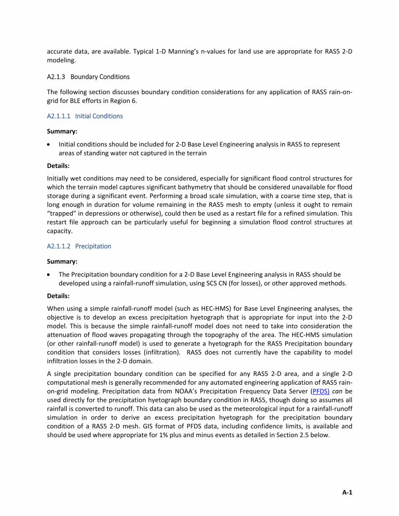
A‐1
accurate data, are available. Typical 1‐D Manning’s n‐values for land use are appropriate for RAS5 2‐D modeling.
A2.1.3 Boundary Conditions
The following section discusses boundary condition considerations for any application of RAS5 rain‐on‐grid for BLE efforts in Region 6.
A2.1.1.1 Initial Conditions
Summary:
Initial conditions should be included for 2‐D Base Level Engineering analysis in RAS5 to represent areas of standing water not captured in the terrain
Details:
Initially wet conditions may need to be considered, especially for significant flood control structures for which the terrain model captures significant bathymetry that should be considered unavailable for flood storage during a significant event. Performing a broad scale simulation, with a coarse time step, that is long enough in duration for volume remaining in the RAS5 mesh to empty (unless it ought to remain “trapped” in depressions or otherwise), could then be used as a restart file for a refined simulation. This restart file approach can be particularly useful for beginning a simulation flood control structures at capacity.
A2.1.1.2 Precipitation
Summary:
The Precipitation boundary condition for a 2‐D Base Level Engineering analysis in RAS5 should be developed using a rainfall‐runoff simulation, using SCS CN (for losses), or other approved methods.
Details:
When using a simple rainfall‐runoff model (such as HEC‐HMS) for Base Level Engineering analyses, the objective is to develop an excess precipitation hyetograph that is appropriate for input into the 2‐D model. This is because the simple rainfall‐runoff model does not need to take into consideration the attenuation of flood waves propagating through the topography of the area. The HEC‐HMS simulation (or other rainfall‐runoff model) is used to generate a hyetograph for the RAS5 Precipitation boundary condition that considers losses (infiltration). RAS5 does not currently have the capability to model infiltration losses in the 2‐D domain.
A single precipitation boundary condition can be specified for any RAS5 2‐D area, and a single 2‐D computational mesh is generally recommended for any automated engineering application of RAS5 rain‐on‐grid modeling. Precipitation data from NOAA’s Precipitation Frequency Data Server (PFDS) can be used directly for the precipitation hyetograph boundary condition in RAS5, though doing so assumes all rainfall is converted to runoff. This data can also be used as the meteorological input for a rainfall‐runoff simulation in order to derive an excess precipitation hyetograph for the precipitation boundary condition of a RAS5 2‐D mesh. GIS format of PFDS data, including confidence limits, is available and should be used where appropriate for 1% plus and minus events as detailed in Section 2.5 below.

A‐2
The following outlines the rainfall‐runoff approach for developing excess rainfall hyetograph time‐series for areas modeled by a 2‐D mesh:
1. Develop simple rainfall‐runoff model (HEC‐HMS) with area and CN, or some other loss methods, specified for contributing areas to the RAS5 2‐D mesh.
2. Determine a precipitation depth (from PFDS) and use a NOAA, SCS, or other reasonable storm distribution in the rainfall‐runoff model (HEC‐HMS). Generally 24‐hour storms are recommended, though other duration storms should be considered when matching up flooding along large main stem reaches and incoming tributaries.
3. Use the simulated excess rainfall time‐series as the Precipitation boundary condition for the 2‐D computational mesh.
Point precipitation values or GIS polygons for recurrence interval rainfall durations, can be obtained from the PFDS. These should be used to determine recurrence interval rainfall for modeling within HEC‐HMS. Areal reduction factors should be considered and can be determined using the Rainfall Frequency Atlas of the United States (US Department of Commerce, 1961), better known as TP‐40, or another approved or more appropriate methodology for Region 6 study areas. The areal reduction applied can also be considered in the reasonability and verification process described in Section 2.3.
Figure 2. Area Depth Curves (Hershfield, 1961)
Statewide soils coverages in gridded format, for developing initial CN’s, should be obtained if the study area is large enough to require a prohibitive amount of individual county soil coverage downloads. Statewide soils coverages can also be obtained from NRCS’s Web Soil Survey at this link:
https://gdg.sc.egov.usda.gov/GDGOrder.aspx?order=QuickState
A Land use‐Soils‐CN matrix can be used to determine CN’s for a particular study area. Table 1 details a typical matrix for determining CN’s for the intersection of soils, land use, and drainage areas, in order to develop a weighted CN for a drainage area. The CN values are sourced from the NRCS’s TR‐55 (USDA 1986). This matrix is intended as a general guide, and should be adjusted based on engineering judgment for a given study area.

A‐3
Table 1: Typical Land use‐Soils‐CN Matrix
LU_GridCode NLCD LU Description Hydrologic Soil Group
A B C D
11 Open Water 99 99 99 99
21 Developed Open Space 49 69 79 84
22 Developed Low Intensity 61 75 83 87
23 Developed Medium Intensity 81 88 91 93
24 Developed High Intensity 89 92 94 95
31 Barren Land 39 61 74 80
41 Deciduous Forest 30 55 70 77
42 Evergreen Forest 30 55 70 77
43 Mixed Forest 30 55 70 77
52 Shrub Scrub 30 48 65 73
71 Herbaceous 49 62 74 85
81 Hay Pasture 39 61 74 84
82 Cultivated Crops 51 67 76 80
90 Woody Wetlands 72 80 87 93
95 Emergent Herbaceous Wetlands 72 80 87 93
A2.1.1.3 Upstream
Summary:
Inflow hydrographs developed for significant drainage areas outside of the 2‐D model mesh should be developed within HEC‐HMS (HMS), using SCS CN (for losses) and Lag Time (for transform), or other approved methods. However, when gage data is available, this should drive the hydrologic modeling, whether maintaining a rainfall‐runoff approach or applying the gage unit hydrograph approach.
Areal reduction factors should be used to reduce the recurrence interval precipitation values for all precipitation events modeled within HEC‐HMS. These will be based on the drainage area to which that rainfall is applied, as well as engineering judgment, particularly with regards to verification of 2‐D model results.
Details:
The overall shape of a 2‐D mesh will depend on the study area (e.g. within a watershed or county), the topography, and the extent of the terrain model. Ideally, models will be setup on an entire watershed to fully utilize the benefits of a rain‐on‐grid approach and to capture all the contributing runoff within the study area. It may be appropriate or necessary to reduce the size of the 2‐D mesh and to use inflow hydrographs for particular flooding sources extending beyond the mesh boundary. In these cases, inflow

A‐4
hydrographs should be developed, as described below, using rainfall‐runoff modeling or applying the unit hydrograph approach to gage data, and then input into the RAS5 model.
Contributing drainage areas can be modeled in a number of ways. Rainfall‐runoff modeling (e.g. HEC‐HMS) is any acceptable method for computing excess precipitation and inflow hydrographs. USGS gage analysis discharges, paired with dimensionless unit hydrographs, provides another method, with the added benefit of supporting verification of hydraulic model results. Upstream boundary conditions, such as an inflow hydrograph, should be developed based on the procedures outlined below. Figure 3 displays a typical situation where inflow hydrographs were derived and applied to the computational 2‐D mesh, shown in blue. The 2‐D area, shown in red, covers the study area, county boundary in grey, for which an excess precipitation should be applied.
Figure 3. Applying Inflow Contributions
Similar to the approach defined in Section 2.1.3.2 for developing excess rainfall hyetograph, the following outlines the rainfall‐runoff approach for developing an inflow hydrograph for areas upstream of modeled 2‐D mesh:
1. Develop simple rainfall‐runoff model (HMS) with area, CN, and lag, or some other loss and transformation methods, specified for a sub‐basin that represents the upstream watershed.
2. Determine a precipitation depth (from PFDS), select a reasonable areal reduction to the rainfall total(s), and use a NOAA, SCS, or other reasonable storm distribution in the rainfall‐runoff model.
3. Use the computed runoff hydrographs for inflow hydrograph boundary conditions to the 2‐D flow area.

A‐5
The unit hydrograph approach for inflow locations with sufficient peak streamflow and observed historical record should be used in lieu of a rainfall‐runoff simulation. This approach involves the following procedure:
1. Perform a flood frequency analysis, using Bulletin 17B procedures (or other approved methods) to determine the magnitude of recurrence interval discharges of interest.
2. Utilizing observed event record, several large events should be selected, with preference given to relatively simple, single‐peak hydrographs.
3. Convert the observed event hydrographs to dimensionless hydrographs by computing the time and discharge ordinates as t/tp and q/qp (where tp is time to peak, qp is peak discharge), and align the dimensionless hydrographs.
4. Determine an average q/qp and t/tp to derive an average dimensionless hydrograph which can be used for developing scaled hydrographs for recurrence interval discharges determined in the gage analysis.
5. Use these gage‐derived outflow hydrograph(s) for upstream inflow hydrograph boundary conditions to the 2‐D flow area.
When modeling very large areas, multiple 2‐D models may be necessary. Outflow hydrographs from upstream rain‐on‐grid models as inflows for downstream adjacent models should be used. If gage information is available for reasonability checks and verification, use these locations as 2‐D flow area boundary locations.
A2.1.1.4 Downstream
Summary:
2‐D meshes should have an obvious location for the downstream outlet, which does not create an artificial backwater
Details:
At a minimum, all 2‐D meshes should have an outlet for flow to leave the system. In some cases, the outlet boundary condition line(s) can extend around a very large portion of the mesh. However, an ideal mesh will have a single obvious location for the downstream outlet. All 2‐D meshes should have at least a single outlet boundary condition, such as normal depth, which does not create any artificial backwater. A gage rating curve at or near the downstream boundary of the model is recommended for use as the model downstream boundary condition, whenever available.
A2.2 Model Controls
The following sections provide discussion and recommendations for RAS5 model controls.
A2.2.1 Mesh Area
Summary:
Due to the limitations of RAS5 2‐D meshes should be limited to less than one million computational cells.
The size and orientation of each 2‐D model mesh should be designed to best represent the area modeled using the rain‐on‐grid approach.
Emphasis should be given to the location of flow and level gages.

A‐6
Details:
RAS5 2‐D meshes can be developed by leveraging GIS to simply and smooth the extents of 2‐D domains. This reduces the need for edits within RAS5 to resolve errors associated with mesh triangulation.
It is recommended that when defining a mesh area complex shapes are avoided or smoothed to avoid triangulation issues and problematic model results. One method to define a suitable mesh area is to digitize a polygon in a GIS package and paste the polygon coordinates directly into the Storage Area Outlines table which creates a Storage Area in the RAS5 Geometry Editor. The Storage Area Outline boundary is then converted to the 2‐D mesh boundary using the “covert to 2‐D area” function.
If irregular edges are present in a 2‐D mesh boundary mesh triangulation issues are likely and further modifications will be required. These issues can be avoided by smoothing and simplifying a jagged‐edged polygon before converting feature vertices to points. Localized mesh errors following smoothing can be addressed by manually modifying the mesh cells using inbuilt geometry modification tools in the Geometry Editor.
A2.2.2 Cell Size Selection
Summary:
It is recommended that for 2‐D Base Level Engineering analyses in RAS5, an initial nominal mesh cell size of 200ft2 is used. This value may be altered depending on the size of the study area, stability issues and model run times.
Details:
For accurate rain‐on‐grid modeling the underlying terrain model must adequately represent the topography of the study area. In RAS5, 2‐D mesh cell faces are represented as cross‐sections, with hydraulic area‐elevation tables computed and stored for each cell in the 2‐D domain.
Differences between digital terrain data resolution and 2‐D mesh cell size is driven by the purpose of the modeling, size of the study area and computational limitations. For applications of RAS5 for Base Level Engineering analyses in Region 6 a 200ft2 mesh cell size is a reasonable starting point from which the mesh can be further refined based on initial runs. Specific watershed topography, flood flow routes and gage locations should inform both 2‐D mesh orientation and cell size.
Due to computational limitations in RAS5 generated 2‐D meshes should be limited to less than one million cells. Determining a mesh cell size involves striking a balance between modeling and mapping accuracy requirements, the resolution of the underlying topography, model run times, hardware and software limitations and model stability at a specific time step.
The specified mesh cell size should be a sufficiently high resolution to accurately capture flood flow routes within the study area and produce stable computations. A number of model iterations should be run during the development process to ensure the most robust and accurate results are produced.
A2.2.3 Time Step Selection
Summary:
When undertaking 2‐D Base Level Engineering analyses in RAS5 a computational time step that balances computational efficiency and produces stable model results should be selected. A suitable time step should be selected using the equation detailed below. The computational

A‐7
time step (T) should be determined using the average cell spacing, X, and the flood wave velocity, V.
Details:
The RAS5 User’s Manual states that Courant number values should be less than or equal to 1.0 although values as high as 3.0 can be allowable when using the Full Momentum equations., When using Diffusion Wave equations Courant number values should be less and or equal to 2.0, while values as high as 5.0 can provide sufficient accuracy . Generally, the computation time step should be small enough such that the time required for water to move through any cell exceeds the time step. Most importantly, the time step used must be sufficient to produce stable results, which can be assessed quickly by viewing stage and discharge hydrographs within a 2‐D mesh. Any numerical noise in either the stage or discharge across a 2‐D cell is indicative of instability within the model.
In 2‐D BLE modeling a simulation time step (in seconds) should not exceed 0.15 multiplied by the nominal 2‐D mesh cell size (e.g. for a 200ft nominal cell size, this equates to a simulation interval of 30 seconds).
Striking a balance between model accuracy and computational time is an important requirement of the RAS5 2‐D modeling process. Whilst reducing the 2‐D timestep may improve model stability in problematic areas of the 2‐D domain this may be to the detriment of model run times. The modeler should seek to refine the 2‐D model mesh in areas of instability rather than simply reducing the timestep which can cause more serious or widespread issues to be masked. Localized stability problems can usually be mitigated by improving mesh representation through the addition of breaklines in areas of rapidly undulating topography.
A2.2.4 Equation Selection and Other Computation Settings
Summary:
Any 2‐D Base Level Engineering analyses in RAS5 should primarily use the Diffusion Wave equations. The Saint‐Venant equations may be leveraged if results derived using the Diffusion Wave equations prove unsatisfactory. Such a decision should be based on a review of model outputs.
Model conservation of volume errors less than 1.0% should be considered acceptable.
Hydrograph and Model Output intervals will initially be set at values significantly larger than the model timestep. These will be adjusted in accordance with scope of work requirements.
An initial broad scale coarse resolution simulation is recommended to define both an end of simulation time that captures the full outfall hydrograph and development of a suitable mesh resolution.
Details:
Once a suitable terrain has been generated using RAS Mapper, a 2‐D mesh can be created within the Geometry Editor. In addition, boundary conditions, and initial conditions can be set and a RAS5 rain‐on‐grid simulation can be undertaken. A balance must be struck between 2‐D mesh resolution and computational runtime. Six significant factors should be considered when striking this balance. These are:
1. The 2‐D mesh computational area;

A‐8
2. The 2‐D mesh cell size;
3. Computational timestep;
4. Simulation duration;
5. Output intervals and variables; and,
6. Equation selection
It is recommended that a broad scale model run be undertaken utilizing a coarse timestep to determine the time at which the flood peak has passed through the outflow hydrograph at the downstream extent of the model This will govern the simulation duration to be set up in the higher resolution model. The start of a simulation should coincide with either inflow entering the 2‐D mesh at the model boundary or the excess rainfall hyetograph being applied to a 2‐D mesh.
As previously discussed a simplified set of equations, known as the Diffusion Wave equations, are typically leveraged where inertial forces dominate frictional and other forces. Where results prove unsatisfactory and flow regimes transition from subcritical to supercritical conditions the Saint‐Venant equations should be utilized.
The RAS5 User’s Manual states that the simplified equation set is usually sufficient for purposes such as flood inundation applications. Overall the Diffusion Wave equations are considered to provide a sufficient balance between model stability and runtime. If the Saint‐Venant equations for shallow flow are selected for use in 2‐D computations then significant increases in model runtimes are likely. Overall a volume percentage error of less than 1% is considered acceptable.
Within RAS5 HDF files are generated for each simulation. It is recommended that the interval for hydrograph outputs be set large enough to minimize unnecessary hard drive data writing, while fine enough to capture useful stage and flow hydrographs. An output interval of 60 minutes or more may be suitable for initial coarse simulations. Output Options can be accessed from the Options menu of an Unsteady Flow Analysis Plan window. Ultimately, the final Hydrograph‐ and Mapping Output Intervals become part of the 2‐D product so all of these settings should be considered before post‐processing.
A2.2.5 Internal 2‐D Mesh Connections
Summary:
Internal 2‐D connections should be added into the 2‐D Base Level Engineering model in RAS5 at stream gage locations. This will allow direct comparison between stage and level gaged data as part of the calibration process.
Reservoirs, particularly those known to provide significant flood control storage, should have internal connections defined. Such results can then be compared with operation and gaged information if available.
Details:
This section details internal connection functionality within RAS5 that should be considered for any application in Region 6 2‐D BLE modeling.
Stage and discharge hydrograph time‐series data at various locations within a 2‐D mesh are valuable for comparing RAS5 rain‐on‐grid results with gaged data and anecdotal evidence. In order to provide locations for reporting stage and discharge hydrographs, RAS5 breaklines should be created and

A‐9
converted to 2‐D internal connections. Terrain profiles along internal connections can be informed by either underlying terrain information or topographical survey.
Breaklines can be defined by importing georeferenced polyline shapefiles via the GIS Tools of the Geometry editor. These breaklines can be converted to Internal Connections by selecting the “convert this Break Line into a new internal SA/2‐D Area Connection” function. The number of internal connections should be sufficient for validating the rain‐on‐grid results. As discussed previously stream gages in the study area are optimal locations to add internal connections. It is good modeling practice to include one internal connection for every 50 square miles of model area. The 2‐D internal connections created in this process are essentially 1‐D cross‐sections conveying flow between 2‐D mesh cells.
Internal connections should also be generated for significant reservoirs within a 2‐D mesh. Spillway geometries can be obtained from terrain data or as built information where available. Storage behind an embankment that would not be available during a flood event should be excluded from any model considerations. A restart file can be used to establish initial water levels in a 2‐D domain for large open water bodies.
Where 2‐D results at dams and reservoirs appear unrealistic gate and culvert openings can be included as internal connections to help improve model performance
A2.3 Reasonability and Verification Checks for the 1%‐Annual‐Chance Event
Summary:
Multiple iterations of the 2‐D Base Level Engineering analysis in RAS5 should be run until WSELs and discharges are deemed reasonable based on engineering judgment.
Verification checks should be informed by the most robust available data such as gaged records. Further verification measures should be driven by the quality and availability of pertinent data.
There will often be instances where reservoirs, particularly those providing significant flood control storage, can be considered as verification locations within a model.
Verification checks for locations without gage estimates should use the best available data, including model‐backed effective AE and A Zone flooding, regression equation estimate ranges, anecdotal evidence of flooding and even adjacent watersheds with available gage estimates.
Details:
The following section provides an overview of the approach for checking the robustness of results derived from a RAS5 rain‐on‐grid simulation. Although this procedure is suggested for BLE application of RAS5, it is also recommended for the Regulatory Approach for converting to Zone A SFHAs. It should be noted that the Base Level Engineering Approach may not warrant more than a single iteration or two to reach satisfactory reasonability based upon the project specifics.
The hydrologic input in the RAS5 2‐D Base Level Engineering analysis is rainfall. When using a simplified rainfall‐runoff model for Base Level Engineering analyses, the objective is to develop an excess precipitation hyetograph that can be applied directly to the 2‐D domain as opposed to trying to match simulated recurrence interval peak discharges to those computed from a gage analysis. This is because the simplified rainfall‐runoff model does not take into consideration the attenuation of flood waves propagating through the watershed. The HEC‐HMS simulation (or other rainfall‐runoff model) is performed to generate a hyetograph for the RAS5 Precipitation boundary condition that considers losses (infiltration), since RAS5 does not have this functionality in its current version.

A‐10
Important reasonability checks involve comparing the WSELs and flood boundaries from the 2‐D model with the following:
Associated stage and discharge from a gage analysis;
Observed data from previous flood events
Existing/effective WSELs and boundaries (primarily from model‐backed Zone AE and Zone A studies);
Other anecdotal information that may be available
The 2‐D model results may not compare favorably with effective Zone A boundaries, due to the outdated methodology associated with many effective Zone A studies. The 2‐D Base Level Engineering analysis represents a more sophisticated and credible approach, and as such should be expected to vary from many of the legacy effective Zone A floodplains. Model‐backed Zone A studies can be used for verification of model results and efforts should be made to tie into effective, model‐backed floodplain boundaries.
When assessing the suitability of gaged estimates for verification, consideration must be given to the unregulated or regulated nature of the record. This is also true for using verification locations which are considered unregulated and downstream of regulated gage records. Care must be taken to ensure proper comparisons are being made between gage estimates and 2‐D model results.
All reservoirs, particularly those providing significant flood controls, should be considered for points of verification. Embankments and spillways commonly n have gaged data with significant record lengths.
Also, it is common that LiDAR‐based terrain models capture the normal retention level of a significant reservoir, depending on the operation of the reservoir and time during which the LiDAR was collected. Consideration should be given to how water bodies are represented within a 2‐D domain, particularly if they are designed to offer flood protection during a significant event.
When effective data is not available for use in verification, regression equation estimates can be used as a guide for determining if further adjustments are needed to improve verification results. Specifically, the range of discharges computed using the standard error range of applicable regression equations can be compared with 2‐D model results at verification locations.
However, it will not be uncommon for discharges to vary wildly, while actual WSELs would not. If effective detail data is available, then these WSEL’s and boundaries should generally take precedence over all other measures. The only exception being gaged estimates with sufficient record length of at least 10 years and preferably 20 or more years.
The following reflects the minimum approach that will be followed to perform checks to verify that the results from the 2‐D RAS5 model are reasonable:
1. Compare resulting RAS5 1%‐annual‐chance WSELs, flood extents, and peak discharges with best available data at the Stage and Discharge comparison lines discussed in Section 2.2.5.
2. Using engineering judgment, adjust Curve Numbers within the HEC‐HMS model and regenerate an excess precipitation time‐series for use as the precipitation boundary condition in RAS5. If the unit hydrograph approach is employed for deriving inflow hydrographs, the timing of these can be adjusted based on engineering judgment.
3. Evaluate if any significant features are not accounting for in cell wall locations. Breaklines may need to be added or adjusted to appropriately account for storage within the 2‐D mesh area.
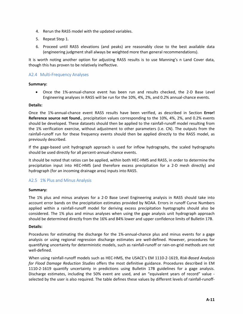
A‐11
4. Rerun the RAS5 model with the updated variables.
5. Repeat Step 1.
6. Proceed until RAS5 elevations (and peaks) are reasonably close to the best available data (engineering judgment shall always be weighted more than general recommendations).
It is worth noting another option for adjusting RAS5 results is to use Manning’s n Land Cover data, though this has proven to be relatively ineffective.
A2.4 Multi‐Frequency Analyses
Summary:
Once the 1%‐annual‐chance event has been run and results checked, the 2‐D Base Level Engineering analyses in RAS5 will be run for the 10%, 4%, 2%, and 0.2% annual‐chance events.
Details:
Once the 1%‐annual‐chance event RAS5 results have been verified, as described in Section Error! Reference source not found., precipitation values corresponding to the 10%, 4%, 2%, and 0.2% events should be developed. These datasets should then be applied to the rainfall‐runoff model resulting from the 1% verification exercise, without adjustment to other parameters (i.e. CN). The outputs from the rainfall‐runoff run for these frequency events should then be applied directly to the RAS5 model, as previously described.
If the gage‐based unit hydrograph approach is used for inflow hydrographs, the scaled hydrographs should be used directly for all percent‐annual‐chance events.
It should be noted that ratios can be applied, within both HEC‐HMS and RAS5, in order to determine the precipitation input into HEC‐HMS (and therefore excess precipitation for a 2‐D mesh directly) and hydrograph (for an incoming drainage area) inputs into RAS5.
A2.5 1% Plus and Minus Analysis
Summary:
The 1% plus and minus analyses for a 2‐D Base Level Engineering analysis in RAS5 should take into account error bands on the precipitation estimates provided by NOAA. Errors in runoff Curve Numbers applied within a rainfall‐runoff model for deriving excess precipitation hyetographs should also be considered. The 1% plus and minus analyses when using the gage analysis unit hydrograph approach should be determined directly from the 16% and 84% lower and upper confidence limits of Bulletin 17B.
Details:
Procedures for estimating the discharge for the 1%‐annual‐chance plus and minus events for a gage analysis or using regional regression discharge estimates are well‐defined. However, procedures for quantifying uncertainty for deterministic models, such as rainfall‐runoff or rain‐on‐grid methods are not well‐defined.
When using rainfall‐runoff models such as HEC‐HMS, the USACE’s EM 1110‐2‐1619, Risk‐Based Analysis for Flood Damage Reduction Studies offers the most definitive guidance. Procedures described in EM 1110‐2‐1619 quantify uncertainty in predictions using Bulletin 17B guidelines for a gage analysis. Discharge estimates, including the 50% event are used, and an “equivalent years of record” value ‐selected by the user is also required. The table defines these values by different levels of rainfall‐runoff‐

A‐12
routing model complexity and agreement with observed data. These are generally in increments of 10 years, with 10 years being the smallest value.
The rainfall‐runoff modeling defined for 2‐D BLE in this guidance is a simplification of a rainfall‐runoff (no routing) simulation to address the lack of infiltration modeling functionality in the current version of RAS5. No routing or attenuation is considered, and model parameters are often revised significantly during the RAS5 model reasonability and verification process. For 2‐D BLE in Region 6, Antecedent Runoff Condition (ARC) II CN’s should be used for the 1% event and ARC III CN’S for 1% plus rainfall‐runoff event estimate. The 1% minus event should be computed using CN’s assuming ARC 1.5 conditions, halfway between ARC I and ARC II conditions as shown in Figure 4 below).
Figure 4. Plot of ARC I, ARC 1.5, and ARC III versus ARC II
A review of previous studies indicated the 1% minus event is generally of lower magnitude than the 10%‐annual‐chance event using hydrologic methods other than a gage analysis; therefore it is recommended that ARC 1.5 be used for the 1% minus event. It is also recommended that the discharge estimates simulated (via rainfall‐runoff modeling) for the 1% minus event should be based on the combination of the rainfall and CN adjustments. These should not exceed the simulated estimate for the 10%‐annual‐chance event. Engineering judgment should also be part of final determination for the CN adjustment, and deviations from the recommendations documented. The unit hydrograph approach involves gage analyses, for which CN and rainfall adjustments do not apply.
The conversion from a normal Antecedent Runoff Condition (ARC II) to a wet (ARC III) or dry (ARC I) condition is provided in Table 10‐1 of the Hydrology section of the NRCS’s National Engineering Handbook, and included in Figure 5, below. The same information is also provided in graphical form in Error! Reference source not found. below.

A‐13
Figure 5. Table 10‐1 and Figure 10‐4, Chapter 10 of NRCS’s NEH‐4
It is recommended that rainfall inputs be adjusted, whether directly on a 2‐D mesh or within HEC‐HMS over a sub‐basin, to model 1% plus and minus events. When using a rainfall‐runoff simulation to develop an excess precipitation hyetograph or inflow hydrographs for upstream boundary conditions, adjustments to CN’s should also be considered. These adjustments should seek to achieve ranges in rainfall‐runoff simulated peak discharges similar to that of a gage analysis or regression equations used in the study area.
As RAS5 can only use a single precipitation value for each 2‐D flow area, point rainfall values from the NOAA PFDS can be applied (either directly from the PFDS or via an area‐weighted determination from PFDS GIS data). In addition to recurrence interval precipitation estimates, NOAA Atlas 14 provides 90% confidence intervals of reported precipitation values, as shown in Figure 6.
Figure 6. NOAA Atlas 14 Precipitation Values

A‐14
On a normal distribution curve, 90% confidence intervals correspond to +/‐ 1.645 standard deviations (i.e. 5% on each tail). The 1% plus and minus events are defined to be one standard deviation above and below the 1%‐annual‐chance event. It should be noted that the error bands for the selected rainfall depth should be applied to the precipitation value used in modeling post‐areal reduction. An example of the calculation process for a point depth of 5.56 inches is provided in Table 2 below.
Table 2: Point Depth Calculation Example
1% Precipitation: 5.56 in
90% Upper Limit: 7.02 in
90% Lower Limit: 4.34 in
Difference (3.29 st. dev.): 2.68 in
1 st. dev.: 0.81 in
1% Plus Precipitation: 6.37 in
1% Minus Precipitation: 4.74 in
The 1% plus and minus event precipitation totals can be determined using PFDS data, specifically of confidence limits. Using GIS data instead of point rainfall totals differs only in that GIS data provides a spatial understanding and area‐weighted determination for a point depth estimate.
Precipitation Data: NWS/NOAA Precipitation Frequency Data Server
GIS Precipitation Data: PFDS in GIS format (including confidence limits)
A2.6 Model and Mapping Outputs
Geometry and plan run data are stored in the .gXX.hdf and .pXX.hdf files, respectively. The size of the plan .hdf file depends on the Computation Settings, as described in Section 2.2.4. These include the Hydrograph, Mapping, and Detailed Output Intervals.
Summary:
Depth and WSEL grids will be exported for each flood event analyzed utilizing the “Sloping (interpolated)” rendering feature.
Velocity grids will be exported for the 1%‐annual‐chance event.
Details:
For the Base Level Engineering Approach, the Hydrograph Output Interval should be frequent enough to capture any model stability issues associated with stage profiles and discharge hydrographs produced during the simulation. The Mapping Output Interval is used for dynamic mapping (animating in RAS Mapper) of model results. This interval must be equal to or larger than the Hydrograph Output Interval, and the interval to use depends primarily on the visualization requirements of the study. The Detailed Output Interval for a Base Level Engineering Approach can be set to a very large interval, unless detailed information of the computations is important for the study.
Depth and WSEL grids for the 10%, 4%, 2%, 1%, 0.2%, 1% plus, and 1% minus annual‐chance events should be exported, and included within the default model subfolders, for any multi‐frequency RAS5

A‐15
rain‐on‐grid model. The “Sloped” rendering mode should be selected from the Render Mode options window and used for these mapping exports. Inundation boundaries can also be exported from RAS Mapper. Generating the flood boundaries is an optional task when utilizing the Base Level Engineering Approach.
A2.7 Mapping Post‐Processing
Summary:
Flood risk areas focused on established CNMS or Effective Mapping products
Additional raw model outputs retained and categorized for informational purposes
Seamless product covering entire project footprint
Figure 7. Boundary Creation Workflow
Details:
Rain‐on‐grid 2‐D modeling produces a product that calculates a depth at nearly every cell. While there may be depths associated with numerous raster cells, they may not all necessarily be deemed as a floodplain. These broad overview steps will help filter the raw results down to the proposed flood risk areas. The flood risk polygons will be based off of existing CNMS features and effective floodplains.

A‐16
Initial Automated Mapping Cleanup steps:
1. Convert Depth Raster to polygon feature class or shapefile
a. Simplify polygons – removes extraneous bends while preserving essential shape
b. Smooth polygons – smooths sharp angles in polygon outlines to improve aesthetic or cartographic quality; Suggested Smoothing Tolerance = 2.5x input raster cell size (i.e. 10ft raster = 25ft Smoothing Tolerance)
2. Create a “scope” layer that will be used to identify our extents of proposed flood risk areas
a. CNMS Unknown, Unverified, and Unmapped
b. Effective flood zones from NFHL or FEMA Q3 digital data
3. Use a minimal buffer to select raw model polygons that intersect our “scope” layer
4. All Additional flood polygons should be retained in a separate layer and should contain a categorization of Greater Than or Less Than 1 foot
Manual Mapping Considerations:
At this point, the floodplain mapping cleanup becomes much more of a manual process rather than automated. The 2‐D results can vary from study area to study area due to a number of reasons, and a one‐size‐fits‐all approach cannot always be taken. For example, areas that are extremely flat, have low velocities, and have very shallow depths can create unique challenges. In these situations, if setting the initial depth threshold to 0.1ft can remove a significant amount of ‘noise’ in a floodplain while retaining the CNMS identified features, then that step can be taken. When the selection of data for the proposed flood risk areas does not capture a portion of the floodplain, a manual selection and incorporating into the proposed flood risk dataset is needed. Typical GIS mapping cleanup processes will be undertaken to address these situations on a case‐by‐case basis. Aerial imagery will also be used as needed to help support these activities. Similar to other mapping projects, small islands within the mapped floodplain will be filled in as appropriate.
Tie Ins:
Since the modeling is not done at county wide level, the mapping of work areas will need to be reviewed for proper tie‐ins. The floodplain data will ultimately be submitted as a county‐wide layer, but should be a seamless feature that will connect across political boundaries. The use of the same county boundary shapefile for these submittal extents should be used. Floodplains from adjacent work areas will need to be checked as well for connectivity and to create the seamless layer.
All CNMS Valid Zone AE studies will be identified and the proposed Zone A flood risk areas will tie into those areas. The data to tie into will come from NFHL as the top priority, but if not available in that dataset, the FEMA Q3 data should be used.

A‐17
A2.8 CNMS Zone A Validation
When the 2‐D BLE assessment data has been compiled, the following procedures should be used for completing the Zone A validation assessment check A5 (Refined Zone A Engineering Comparison). Additional Zone A validation assessment steps and CNMS integration procedures are required for all BLE studies and are described in the CNMS Database Section of R6 BLE Submittal Guidance.
Summary:
To validate the effective Zone A polygons using 2‐D outputs, the required datasets are:
Ground Elevation Grid
1%(+) Water Surface Elevation Grid OR 2‐D mesh with centroid representation
1%(‐) Water Surface Elevation Grid OR 2‐D mesh with centroid representation
Effective Zone A Polygons o Use NFHL Data if available. If not, use Q3 or best available digital representation of
effective Zone A boundaries
The fundamental evaluation procedure is to create a “confidence band” by using the 1%(+) and 1%(‐) values and determining if the effective boundary is mapped within it. Simply put, if the effective Zone A floodplain boundary falls in that range, it passes. If it does not fall within it, it fails. In keeping with the approach outlined in the Automated Engineering Guidance document (May 2016), an allowable horizontal offset tolerance is applied to help in these checks.
Details:
Create Test points
Create Test points along effective Zone A boundary lines spaced at an interval of 500‐ft.
Create the Confidence Band
To create the minimum value of the band, extract the minimum elevation from the 1%(‐) grid. To account for an allowable vertical tolerance, the minimum value should be lowered by that amount. For Region 6 specifically, a vertical tolerance of 2.5‐ft was used based on assumed effective topological data.
To create the maximum value of the band, extract the maximum elevation from the 1%(+) grid. To account for an allowable vertical tolerance, the minimum value should be lowered by that amount. For Region 6 specifically, a vertical tolerance of 2.5‐ft was used based on assumed effective topological data.
Assign Effective Zone A Boundary Elevation
If we assume that the boundary is the same as where the 1% WSE meets the ground, we can use the value from the ground to equal our tested 1% WSE.
Extract Ground values and populate that value into the test point.
Perform Validation on the Test Points
Determine if each test point ground elevation is within the confidence band that was created earlier.
If point value is within the band, it passes. If it is not within the band, it fails.

A‐18
Figure 8. Profile Example of Validation Results
Report Validation results
The spatial test points pass/fail rates can be aggregated and reported on a stream basis for reporting in CNMS.
The spatial test points pass/fail rates can also be aggregated and reported on a County basis or a HUC‐12 basis for reporting measures (or perhaps HUC‐10 or HUC‐8 levels).See the CNMS Database Section of R6 BLE Submittal Guidance for additional instructions on integrating results into CNMS, including A1‐A4 validation checks, unmapped line integration, populating BLE tracking fields, and Status Type updates.

A‐19
A‐3 Additional Considerations
There are considerations to be made for converting the Base Level Engineering Approach products to a level suitable for regulatory purposes. This section discusses pertinent enhancements to the models developed in the Base Level Engineering Approach that should be considered, primarily in the context of 2‐D BLE efforts. However, the modeling and reviewing engineers retain the final decision on the extent to which applying these enhancements would actually result in a noticeable improvement in model results.
Currently, the greatest limitation of RAS5 rain‐on‐grid is its inability to model infiltration of rainfall for any given condition. The Base Level and Regulatory Approach each address this limitation, via rainfall‐runoff modeling for determining excess precipitation resulting from a recurrence interval flood event. For the Base and Regulatory Approach for large scale modeling, the use of a rainfall‐runoff model, simple or complex, should be in response only to the current lack of infiltration modeling in RAS5. There are, however, opportunities for extending the understanding of runoff response for any watershed that is not covered here.
Greater engineering detail of specific areas within a RAS5 BLE model is a likely interest of stakeholders. Of course, more detailed models can be produced for these areas. However, the BLE approach can be maintained by refining a 2‐D mesh in RAS5, for example, using breaklines, internal connections, internal structures, and manual cell configurations at targeted locations. Improving the definition of risk for particular areas within a work area model seems an appropriate measure for upgrading a 2‐D BLE model to a product suitable for regulatory purposes.
A3.1 Topographic Conditions
This section identifies five distinct regions with significantly different hydraulic behavior and provides the Mapping Partner guidance to perform 2‐D Base Level engineering (BLE) hydraulic analyses for these regions.
A3.1.1 Lowlands/Mississippi River Delta Region
One of FEMA Region 6’s most prominent hydrologic features is the Mississippi River. The river drains approximately one third of the area of the nation’s 48 contiguous states. As such, over a long period of time, the Mississippi River has carved a wide, low‐lying, changing floodplain which empties in the Gulf of Mexico. Roughly along the Illinois and Missouri state line begins what is also known as the Mississippi River Lowlands or Mississippi Embayment. The Lowlands extend south through Arkansas and into Louisiana until they become the Mississippi River Delta. Large flows of water and sediment changed the Mississippi River Lowlands and Delta regions until flood control structures were built that kept the river’s main channel in a fixed location.
A3.1.1.1 Mississippi Lowlands
The Mississippi River Lowlands are a low‐lying, generally flat topographical feature formed over geologic times and can measure over 100 miles across. In 1927, the Mississippi River flooded a significant portion of the lowlands. To prevent another flood of such magnitude, the federal government built a system of levees that prevent the Mississippi River flow from reaching the Lowlands directly. However, the Mississippi River Lowlands maintain many of the features that result from fluvial geomorphology. These features are the result of sinuous and meandering rivers and bayous that once discharged into the Mississippi River. Populated areas often follow “high ground” formed by sediment deposited over

A‐20
geologic times, but the overbank areas are often barely higher than the water level in the channel. As such, when these systems overflow, the result is shallow, lateral flow that can extend for long distances.
As such, the main modeling assumption in the Mississippi River Lowlands is storage. Given an accurate representation of the ground elevations, a two‐dimensional model is well equipped to handle storage and compute depths. However, the accuracy of the topographic data is paramount to the accurate calculation of water depths or water surface elevations because slight deviations on ground elevations can result in significant storage calculation differences. Given the flatness of the terrain, the model mesh resolution may remain coarse. The modeler should use engineering judgment to determine where breaklines should be placed to best represent key obstructions to flow in the 2‐D domain. The development of the terrain model and model mesh are described in Sections 2.1.1 and 2.2.1 of this guidance document.
A3.1.1.2 Mississippi River Delta
Much of the guidance provided for the Mississippi River Lowlands applies to the Mississippi River Delta region. In the Delta region, stream flow tends to split and spread in different directions which a two‐dimensional model can replicate given an accurate topographic data.
As in the Lowlands, many of the channels and ditches have water year‐round. However, in the Delta region, tides may affect the hydraulics of the channels. To this end, the modeler may apply a tidal boundary condition in this location. A value higher than the mean high water tide may help incorporate the effects of storm surge, which may occur simultaneously with a runoff event.
Of note, coastal floodplains in the Delta region may see flooding from rainfall runoff as well as coastal surge elevations. If calculated independently from each other, a flood frequency elevation analysis should incorporate coastal and riverine flood events by adding them statistically through the combined rate of return approach. Use of a joint probability analysis is also appropriate.
A3.1.2 Coastal Regions/Combined Probability
FEMA Region 6 has a long coastline with the Gulf of Mexico along Texas and Louisiana. Characteristic topographic features in these coastal watersheds include low gradients and interior bays (particularly in Texas).
Coastal watersheds often lack a single, defining stream that drains the watershed. Instead, coastal watersheds (including USGS’s HUC‐8 watersheds) often include multiple streams that run relatively parallel to each other (i.e., do not accumulate flow from the entire watershed) before discharging into the ocean or bay. Some of these rivers and bayous may experience interbasin flow transfers, which a two‐dimensional model can simulate well, if the terrain is accurate. As such, the development of a terrain model (described in Section 2.1.1) must show this drainage pattern.
Coastal watersheds are highly influenced by tides and coastal surge levels. The modeler should choose a boundary condition consistent with other FEMA Guidance that considers tides and storm surge. The modeler may use a mean high water tidal datum or a value between the 50‐ to 10‐percent annual chance elevations as a downstream boundary condition. The choice of boundary condition should be carefully considered. Of note, a value higher than the mean high water tide may help incorporate the effects of storm surge, which may occur simultaneously with a runoff event.

A‐21
A3.1.3 Playas/Endoheric Basins
Playas are found in the Southern High Plains of Texas, Oklahoma and New Mexico. Since playas are typically shallow, circular‐shaped wetlands, they are best modeled using 2D methods as the models lend themselves well to more accurately dealing with the storage and attenuation impacts. Special attention should be paid to those playas that have gravity drainage systems. If significant, drainage system capacity/inflow should be modeled to account for the storage in the 2D model. Playas that are simply recharge basins (recharge for the aquifer) do not need to include infiltration information as the 2D analysis will suffice for a BLE study.
A3.1.4 Arid Southwest
Although the hydraulic approach in an arid area would be consistent with the approach described in this document, the hydrology would vary. Due to a lack of extensive gage record, flood frequency analysis is rarely an option. Additionally, regression equations have large standard errors. The approach most favorable is rainfall runoff modeling.
In some locations Drainage Design Manuals have been published which contain area specific methods to be used in areas of arid hydrology. In areas where a drainage design manual is not available, those from nearby areas may contain useful guidance. Within Region 6, Drainage Design Manuals have been published by New Mexico State Highway and Transportation Department and the City of El Paso, TX. Although not in Region 6, Drainage Design Manuals or Hydrologic Modeling Guidelines have been published by Arizona Department of Transportation; Arizona Department of Water Resources; Coconino County, AZ; Yavapai County, AZ; and Flood Control District of Mohave County, AZ.
Of particular note, areal reduction of precipitation is more important in an arid region. The above mentioned resources and Depth‐Area Ratios in the Semi‐Arid Southwest United States (Zehr and Meyers, 1984) can be used to develop the best approach to areal reduction.
A3.1.5 Urban Areas
Terrain model development in urban areas should follow the same procedures outlined in previous sections which require incorporating the main hydrologic features. Urbanized topography often includes roads, railroads, man‐made channels, and numerous culverts and bridges, which determine flow movement. A 2‐D BLE study should not incorporate every single hydraulic structure. However, the modeler should assess the overall flow patterns and include the main hydraulic features only (for example, sharp embankments and man‐made channels) These features can be identified by undertaking a coarse model run and locating area of flow attenuation. Offset breaklines can then be used as an alternative to explicitly modeling the structure in 1‐D.
If a LiDAR dataset that includes buildings is available, the modeler may leave the buildings in the terrain model. A hydraulic model with buildings included as part of the terrain will display flow moving on the streets exclusively and not “through” the buildings. Given that a hydraulic model with bare earth terrain (i.e., without buildings and tree canopy) simulates flow resistance with the aid of Manning’s n values, the modelers should adjust these values accordingly, in the event that the terrain includes buildings.
A3.2 Non‐levee Features
Non‐levee features, such as road or railroads embankments, should not be allowed to simply act as natural high ground or accredited levees within the terrain. The base flood should be allowed to pass through these structures, as appropriate, using either modifications to the terrain or incorporation of

A‐22
hydraulic structures through the feature. The levee guidance being released in the Fall 2017 cycle is planned to include additional guidance regarding this topic.
A3.3 Levees
A levee is an embankment or wall built to contain rising water. Throughout FEMA Region 6, levees of many sizes and conditions exist. Levees with documentation that the criteria of 44CFR65.10 have been met can be accredited, with the FIRM panels showing a reduced flooding risk.
To certify a levee, the owner is responsible for complying with the requirements included in 44CFR65.10. To show reduced risk in areas protected by levees, FEMA must perform a completeness check on the certification package to verify that the certification package is adequate. This section addresses levees modeled for riverine flood sources only, as BLE approaches for coastal are not considered in this guidance.
The official FEMA levee guidance is set to be released in the Fall 2017 cycle and will supersede all current levee guidance, except levee guidance for seclusion and Zone AR/A99. This section provides additional guidance to include levees in a 2‐D BLE study, but does not supersede or replace other specific levee guidance documents.
A3.3.1 Accredited Levees
Accredited levees represent significant drainage features because they constrict flow and direct it elsewhere. Accredited levees have certified data that the levee is designed to withstand at least the 1‐percent annual chance flood.
Accredited levees must be included in the terrain model used to develop a hydraulic 2‐D BLE study. A modeler can accurately describe a levee’s alignment and crest elevation using three‐dimensional breaklines. For a 2‐D BLE study, a detailed cross section geometry of the embankment is not necessary. The modeler must ensure that the levee connects seamlessly upstream/downstream tie‐ins and hydraulic road crossings. If a tie‐in includes a non‐levee feature, rather than high ground, the modeler must take into consideration non‐levee feature approaches, as described in the Fall 2017 guidance.
Results of the 2‐D BLE should be compared against the effective to evaluate how the levee accreditation may be affected by the new analysis. The community should be asked to provide the confirmation that their levee system is still considered accredited against the new base flood elevations that would eventually come into effect from the 2‐D BLE, which may necessitate a revised certification package.
Accredited levees must also be evaluated for residual flood risk and interior drainage. If not part of the 2‐D BLE scope, interior drainage may be carried over from the certification package.
A3.3.1 Non‐Accredited Levees
Non‐accredited levees are those which have not been shown by the community or levee owner to meet the requirements outlined in 44CFR65.10. FIRM panels should not show non‐accredited levees as providing full protection from a 1‐percent annual chance flood.
Before initiating special modeling considerations, non‐accredited levees should be evaluated for hydraulic significance. There are many small levees in Region 6, usually designed for high frequency events in agricultural areas that do not have significance to the 1‐percent‐annual‐chance flood. These can simply be left in the terrain model as they are. However, the Mapping Partner should communicate

A‐23
their presence and the modeling plan for them to project monitor and to the stakeholders, to check for any objections to considering any specific levees as not hydraulically significant.
The development of a 2‐D BLE study with non‐accredited levees should include the collection of best available data and an evaluation of known deficiencies. Non‐accredited levee systems may be broken into reaches, based on shared characteristics of available data, deficiencies (or lack thereof), and hydraulic conditions. Each levee system must, at a minimum, be analyzed for both natural valley and for the levee held in place. Available data and/or discussion with the community may lead to the need to perform analysis by overtopping or structural‐based inundation (breach).
Performing analyses of a non‐accredited levee requires close coordination with FEMA Region 6’s Project Monitor and Levee Lead and local floodplain administrators to identify what makes the levee non‐accredited and how the map can more accurately depict the flood risk. The final reach analysis and mapping decision should be made only after engaging the levee stakeholders. Minimal coordination may consist of a concurrence to simply proceed with natural valley. Otherwise, a Local Levee Partnership Team (LLPT) should be formed to determine if the levee system has reaches that are to be considered for structural‐based inundation, overtopping, freeboard‐deficient, or sound reach. Some procedures require a high level of data to be submitted by the community to show that some conditions of 44CFR65.10 are met. If a levee requires formation of an LLPT and a procedure other than natural valley is being considered, the Mapping Partner should consider if it may be appropriate to rescope the leveed reach from 2‐D BLE to instead be a detailed study and discuss that option with the FEMA Region 6 Project Monitor.
To model the necessary levee scenarios, including with‐levee and natural valley, a 2‐D BLE study may develop more than one terrain for use in the hydraulic model, where the only difference is the levee. The terrain can incorporate the levee alignment and crest elevation using three‐dimensional breaklines. The availability of multiple terrain datasets may help quickly incorporate levees into a study.
Alternatively, two‐dimensional models can incorporate levees as model features, which is an option in some types of 2‐D software. This approach may prove a more efficient modeling method than creating multiple terrain datasets. As with terrain breaklines, the lines that define a levee should incorporate an accurate crest elevation and alignment. In HEC‐RAS 5, the modeler may create different plans (i.e., simulation “scenarios”) that include the different levee alternatives.
The landward area should also be evaluated for interior drainage conditions and, if necessary, modeled and mapped for interior drainage.
A3.4 Other Flood Control Structures
The goal of flood control structures is to guide or regulate flow and, thus, should be included in a 2‐D BLE study. Other than levees previously discussed in this guidance document, flood control structures include, but are not limited to, dams, weirs, and gates.
2‐D BLE studies include dams and levees in a similar way. Modelers may include dams in a hydraulic model by including the embankment or concrete structure into the terrain. Incorporating the exact dam cross section geometry is not necessary in a 2‐D BLE study.
Unlike levees, dams create enclosed reservoirs. Without an outlet, the water would back up behind the dam until the structure becomes overtopped. However, dams have regulated or free flow discharging mechanisms that allow dam operators to control the water level and prevent overtopping of the design flood event. These mechanisms include weirs, spillways, and gates of varying designs. These structures’

A‐24
rating curves are often available and should become part of the 2‐D BLE study as a downstream or internal boundary condition.
A 2‐D BLE study should not incorporate complex dam operational procedures. For example, a BLE simulation should not try to incorporate operation rules that dam operators follow during flood events. Simply, the BLE simulation should include rating curves of fully open gates and uncontrolled spillways. If rating curves are unavailable, the modeler may modify the terrain to allow for uncontrolled flow, or include weir structures that allow the model to calculate outflow. HEC‐RAS 5 allows the inclusion of weir structures in its Geometry module.
Other weirs — inline or lateral — should be included as part of the BLE analysis, if they represent a significant flow regulator at the 1‐percent annual chance level.

A‐25
A‐4 2‐D Base Level Engineering Hydraulic Review QC Checklist
General
Is the product scalable? (i.e., can the model be upgraded to meet regulatory requirements?) Terrrain/Topgraphic Data
Is the model hydrology based on a DEM with an appropriate resolution? (HUC 10 or smaller should use 10‐meter or better. Larger than HUC 10 should use 30‐meter or better.)
Does the model use terrain data at least as current as the current effective study and meet FEMA topo standards?
Is the input topography reasonably dense? (Cell size should be 10‐foot or less.)
Have topographic abnormalities been corrected? (No. drops or rises due to underlying data errors.)
Incoming Hydrographs (HEC‐HMS and/or gage based)
Are the basin delineations reasonable?
Are the curve numbers reasonable and sufficiently documented?
Are the precipitation depths reasonable and sufficiently documented?
Is the time of concentration determination reasonable for all HEC‐HMS subbasin elements?
Was a reasonable temporal storm distribution used?
Was the appropriate areal reduction factor used for any contributing drainage area inflow modeled using rainfall‐runoff?
If PeakFQ is used, was the correct confidence interval used? (Should be 0.84 instead of default 0.95)
Is gage‐based hydrology reasonable? Does the gage‐analysis follow identified best practices for this project? (If USGS report is available for the gages in this area, the same methodology should be applied to this project, or reasons for deviation should be documented.)
Hydrology (Excess Precipitation)
Does the model include all frequencies? (10%‐, 4%‐ , 2%‐ , 1%‐ , and 0.2%‐acf)
Does the model include the 1%‐plus and 1%‐minus flood events?
Was the appropriate areal reduction factor used for the 2‐D mesh?
Are curve numbers reasonable, and sufficiently documented?
Are the incoming hydrographs being applied properly? (location, shapes, timing, etc.)
For hydrographs transferred from one RAS model to a downstream RAS model, are the incoming and outgoing hydrographs being applied a coincident location?
If applicable, does the peak discharge compare favorably to gages or effective studies? If not, have attempts been made to calibrate? (This applies to both the study area and incoming hydrograph models.)
Does the model account for any significant flow‐regulating dams?
Hydraulics
Does the model use public domain software?
Is the 2‐D mesh reasonably sized to limit cell count and obtain reasonable velocities?
Is the timestep appropriate for the mesh size and calculated velocities?

A‐26
Is the source of the roughness coefficients or criteria for selecting default roughness coefficients documented in the report?
Are significant hydraulic structures and embankments accounted for? (i.e., placing breaklines, 2‐D structures, terrain processing, etc.)
Are comparison points/lines (i.e., internal 2‐D connections) captured and compared against applicable benchmarks? (gage, high water mark, effective BFE, etc.)
Are the boundary conditions established, documented, and reasonable?
If applicable, is the transfer line between this model and a downstream model well away from any boundary condition effects?
Are the initial conditions and final conditions reasonable?
Is the mass balance/volume conservation reasonable? (Generally, this is less than 1.0% for RAS5.)
Was the model simulation long enough to pass the entire hydrograph(s) through the model?
Have instances of significant crossing profiles or adverse slopes been investigated for modeling errors?
Mapping Outputs
Do the boundaries appear reasonable?

A‐27
A‐5 Resources
FEMA Guidance may be updated twice yearly. As such, the FEMA Library should always be checked for updates. The following documents provide useful information that should be considered when developing Base Level Engineering products.
Automated Engineering (May 2016)
General Hydrologic Considerations (May 2016)
Elevation (May 2016)
General Hydraulics Considerations (November 2016)
Hydraulics: One‐Dimensional Analysis (November 2016)
Hydraulics: Two‐Dimensional Analysis (November 2016)

A‐28
A‐6 References
ADOT, 2014, Arizona Department of Transportation Highway Drainage Design Manual, Hydrology, 2nd Edition. ADOT, 1993, Arizona Department of Transportation Highway Drainage Design Manual Hydrology, Final Report, March 1993, Report Number FHWA‐AZ93‐281. ADWR, 2007, State Standard for Hydrologic Modeling Guidelines, SS10‐07, prepared by Stantec and JE Fuller for Arizona Department of Water Resources, Flood Mitigation Section, August 2007. Bruner, Gary and CEIWR‐HEC. February 2016. HEC‐RAS River Analysis System, 2D Modeling User’s
Manual Version 5.0. Davis, CA. City of El Paso, 2012, Drainage Design Manual, draft, City of El Paso Engineering Department, June 2012. Never adopted. City of El Paso, 2008, Drainage Design Manual, City of El Paso Engineering Department, June 2008. FCDMC, 2013, Drainage Design Manual for Maricopa County, Arizona, Hydrology, 4th Edition, dated August 15, 2013, publication of the Flood Control District of Maricopa County, Phoenix, Arizona. FCDMC, 2012, Drainage Design Manual for Mohave County, Arizona, Hydrology, 2nd Edition, dated December 12, 2012, prepared by Arid Hydrology & Hydraulics, LLC for Flood Control District of Mohave County, Kingman, Arizona. Hershfield, D. M., May 1961. Technical Paper No. 40. Rainfall Frequency Atlas of the United States. U.S.
Weather Bureau. U.S. Department of Commerce. Washington, DC. Figure 15. Page 6. NMSHTD, 1995, New Mexico State Highway and Transportation Department Drainage Manual, Volume 1, Hydrology, December 1995. U.S. Department of Agriculture. Natural Resource Conservation Service. "Chapter 2 Estimating Runoff."
Technical Release 55: Urban Hydrology for Small Watersheds. 2nd ed. 1986. Table 2‐2a. Page 2‐5. U.S. Department of Agriculture. Natural Resource Conservation Service. National Engineering Handbook
Hydrology. Chapter 10: Estimation of Direct Runoff from Storm Rainfall. July 2004. Table 10.1. Page 10‐6.
U.S. Department of Agriculture. Natural Resource Conservation Service. National Engineering Handbook
Hydrology. Chapter 10: Estimation of Direct Runoff from Storm Rainfall. July 2004. Figure 10‐4. Page 10‐8.
U. S. Water Resources Council. March 1976. Guidelines for Determining Flood Flow Frequency. Bulletin
17B of the Hydrology Subcommittee. Washington, DC.

A‐29
Zehr, R.M. and Myers, V.A., 1984, Depth‐Area Rations in the Semi‐Arid Southwest United States, NOAA Technical Memorandum NWS HYDRO‐40, Office of Hydrology, Silver Spring, MD.