b algorithm 948: daesa — a matlab tool for structural ...tang4/daesafiles/daesasoftware.pdf · b...
TRANSCRIPT
B
Algorithm 948: DAESA — a Matlab Tool for Structural Analysis ofDifferential-Algebraic Equations: Software
NEDIALKO S. NEDIALKOV, McMaster UniversityJOHN D. PRYCE, Cardiff UniversityGUANGNING TAN, McMaster University
DAESA, Differential-Algebraic Equations Structural Analyzer, is a MATLAB tool for structural analysis ofdifferential-algebraic equations (DAEs). It allows convenient translation of a DAE system into MATLAB andprovides a small set of easy-to-use functions. DAESA can analyze systems that are fully nonlinear, high-index, and of any order. It determines structural index, number of degrees of freedom, constraints, variablesto be initialized, and suggests a solution scheme. The structure of a DAE can be readily visualized by thistool. It can also construct a block-triangular form of the DAE, which can be exploited to solve it efficientlyin a block-wise manner.
Categories and Subject Descriptors: I.6.7 [Computing methodologies]: Simulation support systems; G.4[Mathematical software]: Matlab, Algorithm design and analysis
Additional Key Words and Phrases: Differential-algebraic equations, structural analysis, modeling
ACM Reference Format:Nedialkov, N., Pryce, J, Tan, G., 2015. DAESA— A MATLAB Tool for Structural Analysis of DAEs: SoftwareACM Trans. Math. Softw. 41, 2, Article B ( 2015), 15 pages.DOI = 10.1145/2700586 http://doi.acm.org/10.1145/2700586
1. INTRODUCTION
We present DAESA, Differential-Algebraic Equations Structural Analyzer, a MATLABtool for structural analysis (SA) of differential-algebraic equations (DAEs). It allowsconvenient translation of a DAE into MATLAB and provides (currently 18) easy-to-use functions for determining the structural index, the number of degrees of freedom(henceforth referred to as the DOF), the constraints and a solution scheme, and forvisualizing the structure of the DAE. DAESA can also construct a block-triangular form(BTF), which can be exploited for efficient solution in a block-wise fashion.
Our package is applicable to DAE systems of the general form
fi(t, xj and derivatives of them) = 0, i = 1, . . . , n, (1)
where t is the independent variable, and the xj(t) are n state variables. The formula-tion (1) includes high-order systems and systems that are nonlinear in leading deriva-
Author’s addresses: N. Nedialkov and G. Tan, Department of Computing and Software, McMaster Univer-sity, Hamilton, Ontario, Canada. J. Pryce, Cardiff School of Mathematics, Cardiff University, UK.Permission to make digital or hard copies of part or all of this work for personal or classroom use is grantedwithout fee provided that copies are not made or distributed for profit or commercial advantage and thatcopies show this notice on the first page or initial screen of a display along with the full citation. Copyrightsfor components of this work owned by others than ACM must be honored. Abstracting with credit is per-mitted. To copy otherwise, to republish, to post on servers, to redistribute to lists, or to use any componentof this work in other works requires prior specific permission and/or a fee. Permissions may be requestedfrom Publications Dept., ACM, Inc., 2 Penn Plaza, Suite 701, New York, NY 10121-0701 USA, fax +1 (212)869-0481, or [email protected]© 2015 ACM 0098-3500/2015/-ARTB $10.00
DOI 10.1145/2700586 http://doi.acm.org/10.1145/2700586
ACM Transactions on Mathematical Software, Vol. 41, No. 2, Article B, Publication date: 2015.

B:2 Nedialkov, Pryce, Tan
tives. Furthermore, (1) includes systems of ordinary differential equations (ODEs) andpure algebraic systems.
DAESA performs analysis similar to that of the C++ solver DAETS [Nedialkov and Pryce2008; Nedialkov and Pryce 2009]. However, DAETS is not suitable for rapid investiga-tion of DAEs, as it requires C++ knowledge and compiling the user code. The goal ofthis work is to produce a light-weight, easy-to-use tool with convenient facilities forrapidly exploring a DAE’s structure. The present tool is based on Pryce’s SA [Pryce2001] and recent developments by the authors on improving this analysis using block-triangularization of the DAE. The choice of MATLAB is due to its ubiquity and ease-of-use, as well as its operator overloading, which is central to our implementation.
We do not define the terminology we use here, nor present the underlying theory—forthis see the companion paper [Pryce et al. 2013] and the references therein.
This article is organized as follows. Section 2 gives an overview of DAESA. Section 3presents several examples of analyzing DAEs. Section 4 investigates the performanceof this package and the relative amount of work of various parts of it. Conclusions aregiven in Section 5.
2. OVERVIEW OF DAESA
DAESA exploits MATLAB’s operator overloading to process a DAE given by a user-supplied function for evaluating the fi in (1). In particular, it extracts the signaturematrix1 (Σ) and determines for each equation if it is quasilinear in the leading deriva-tives in the sense explained in the companion paper, see also [Nedialkov and Pryce2008].
After the signature matrix is constructed, DAESA finds out if the problem is struc-turally well-posed, and if so, finds a highest-value transversal (HVT) and solves a lin-ear assignment problem to calculate the offsets of the problem, and then determines itsstructural index and DOF. Since it knows the structure of the analyzed DAE, DAESAreduces it to block triangular form (BTF), finds local offsets, and determines blockby block quasilinearity. Based on the offsets and linearity information, DAESA deduceswhich variables and derivatives of them need to be initialized and what the constraintsare.
This package provides functions for reporting the constraints, initialization summary,and a solution scheme, and functions for displaying the original structure of the DAE,as well as for displaying coarse and fine BTFs of the DAE structure.
The DAESA package builds around three classes: sigma, qla, and SAdata. The signaturematrix is obtained by executing the function defining the DAE with objects of the classsigma. The quasilinearity analysis is carried out by executing this function with objectsof the class qla. In both cases, the processing of the DAE is done through operator over-loading of the arithmetic operators and the elementary functions. The SA is performedby the function daeSA. It returns an object of the class SAdata, which encapsulates allthe data obtained from the SA. Each of the remaining DAESA functions takes an objectof this class as a parameter and extracts from it the data it needs. This mechanism(of the main function returning an object, and the remaining functions querying thisobject) ensures simple and consistent function interfaces.
1Concepts explained in the companion paper are typeset in slanted font on first occurrence.
ACM Transactions on Mathematical Software, Vol. 41, No. 2, Article B, Publication date: 2015.
DAESA— a MATLAB Tool for Structural Analysis of DAEs: Software B:3
Remark. The structural index computed by DAESA is an upper bound on the differ-entiation index, and often they are the same. Although successful on many problemsof interest, the underlying SA theory (and DAESA) may fail to determine the correctstructural, and therefore differentiation index on some problems; see e.g. [Pryce 2001;Nedialkov and Pryce 2007].
We could “certify” that the SA is successful, if the system Jacobian J could be shownto be non-singular at a consistent point [Nedialkov and Pryce 2007]. The present tooldoes not compute consistent points and does not evaluate J: it performs symbolic-typeanalysis of DAEs. We plan to incorporate the evaluation of J in a future version ofDAESA.
3. DAESA EXAMPLES
In this section, we illustrate some of the capabilities of DAESA. Namely, we investigatethe SA of DAESA on a simple DAE, the chemical Akzo Nobel problem [Mazzia andIavernaro 2003] (§3.1). We also present results from analyzing a DAE arising frommodeling a distillation column (§3.2), and show how DAESA reports structurally ill-posed (SIP) problems (§3.3). For details, see the DAESA user guide [McKenzie et al.2013], which is also part of the distribution of this package.
3.1. Simple DAE: Chemical Akzo Nobel
We show DAESA’s SA on the chemical Akzo Nobel problem, an index-1 DAE. The equa-tions for this problem are given in §5.1 of the companion paper. The DAESA functionfor evaluating them is displayed in Figure 1.
func t i on f = akzonobel(t,y)k1 = 18.7; k2 = 0.58; k3 = 0.09; k4 = 0.42;K = 34.4; klA = 3.3; CO2 = 0.9; H = 737;Ks = 115.83;r1 = k1*y(1)^4* sqr t (y(2));r2 = k2*y(3)*y(4);r3 = k2/K*y(1)*y(5);r4 = k3*y(1)*y(4)^2;r5 = k4*y(6)^2* sqr t (y(2));Fin = klA*(CO2/H - y(2));f(1) = -Dif (y(1),1) - 2.0*r1 + r2 - r3 - r4;f(2) = -Dif (y(2),1) - 0.5*r1 - r4 - 0.5*r5 + Fin;f(3) = -Dif (y(3),1) + r1 - r2 + r3;f(4) = -Dif (y(4),1) - r2 + r3 - 2.0*r4;f(5) = -Dif (y(5),1) + r2 - r3 + r5;f(6) = Ks*y(1)*y(4) - y(6);
end
Fig. 1. DAESA function for evaluating the chemical Akzo Nobel problem
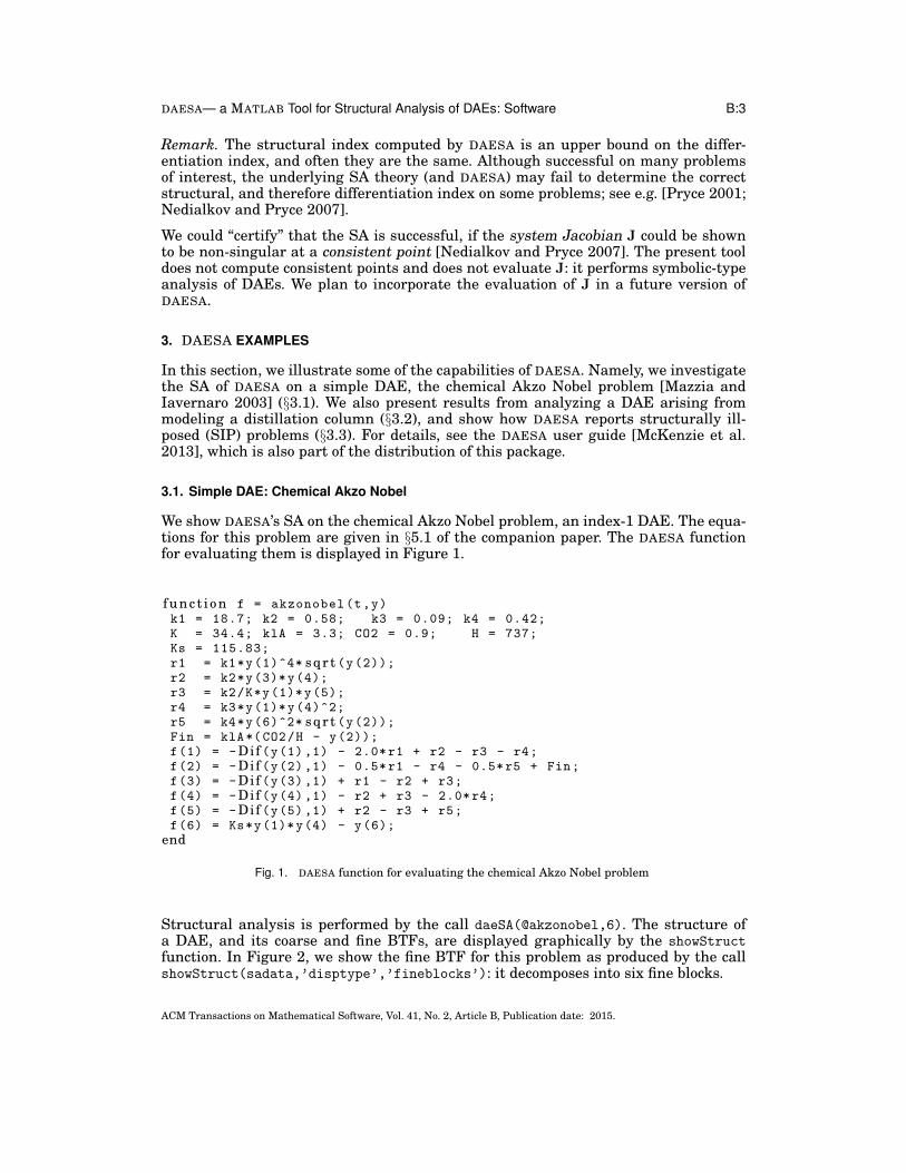
Structural analysis is performed by the call daeSA(@akzonobel,6). The structure ofa DAE, and its coarse and fine BTFs, are displayed graphically by the showStructfunction. In Figure 2, we show the fine BTF for this problem as produced by the callshowStruct(sadata,’disptype’,’fineblocks’): it decomposes into six fine blocks.
ACM Transactions on Mathematical Software, Vol. 41, No. 2, Article B, Publication date: 2015.
B:4 Nedialkov, Pryce, Tan
1 2 3 4 5 6
1
2
3
4
5
6
AKZONOBEL: Fine BTF
Size 6, structural index 1, DOF 5Shaded: structural nonzeros in system Jacobian J
Boxed: positions that contribute to det(J)
1
0
0
0
0
0
0
1
0
0
0
1
0
0
0
0
0
1
0
0
0
0
0
1
0
0
0
1
1
1
1
1
0
0
0
0
0
0
0
0
0
c i
0
0
0
0
0
0
c i
1 1 1 1 1 0d j
1 1 1 1 1 0d j
Indices of Variables
Ind
ice
s o
f E
qu
atio
ns
Fig. 2. Fine BTF and solution scheme for the chemical Akzo Nobel problem
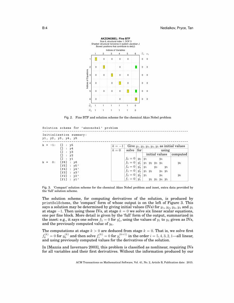
Solution scheme f o r ’akzonobel ’ problem---------------------------------------------------------------------------Initialization summary:y1, y2 , y3 , y4, y5---------------------------------------------------------------------------k = -1: [] : y5
[] : y4[] : y3[] : y2[] : y1
k = 0: [f6] : y6[f5] : y5 ’[f4] : y4 ’[f3] : y3 ’[f2] : y2 ’[f1] : y1 ’
k = −1 Give y1, y2, y3, y4, y5 as initial valuesk = 0 solve for using
initial values computedf6 = 0 y6 y1 y4f5 = 0 y′
5 y1 y2 y3 y4 y6f4 = 0 y′
4 y1 y3 y5f3 = 0 y′
3 y1 y2 y4 y5f2 = 0 y′
2 y1 y4 y6f1 = 0 y′
1 y2 y3 y4 y5
Fig. 3. ‘Compact’ solution scheme for the chemical Akzo Nobel problem and inset, extra data provided bythe ‘full’ solution scheme.
The solution scheme, for computing derivatives of the solution, is produced byprintSolScheme, the ‘compact’ form of whose output is on the left of Figure 3. Thissays a solution may be determined by giving initial values (IVs) for y1, y2, y3, y4 and y5at stage −1. Then using these IVs, at stage k = 0 we solve six linear scalar equations,one per fine block. More detail is given by the ‘full’ form of the output, summarized inthe inset: e.g., it says one solves f5 = 0 for y′5, using the values of y1 to y4 given as IVs,and the previously computed value of y6.
The computations at stage k > 0 are deduced from stage k = 0. That is, we solve firstf(k)6 = 0 for y(k)6 and then solve f (k)i = 0 for y(k+1)
i in the order i = 5, 4, 3, 2, 1—all linear,and using previously computed values for the derivatives of the solution.
In [Mazzia and Iavernaro 2003], this problem is classified as nonlinear, requiring IVsfor all variables and their first derivatives. Without the information produced by our
ACM Transactions on Mathematical Software, Vol. 41, No. 2, Article B, Publication date: 2015.

DAESA— a MATLAB Tool for Structural Analysis of DAEs: Software B:5
BTF it would be regarded as fully coupled, needing solution of a non-linear system ofsize six to determine values for y(k+1)
i , i = 1, . . . , 5, and y(k)6 at stage k = 0, 1, . . ..
3.2. Chemical engineering application: distillation column
Systems of DAEs are commonly used in chemical engineering to describe mass/energybalances and constitutive relations, such as mass/energy transfer rates, reaction ki-netics, thermodynamic properties and relations and control laws. Depending on theassumptions used to construct the model, a DAE system with an index exceeding oneis possible. Then typically an index reduction is performed, and the resulting systemis simulated with a standard, index-1 DAE solver (e.g., SUNDIALS [Hindmarsh et al.2005] or DASSL [Brenan et al. 1996]).
From a modeler’s perspective, one might be interested in determining the indices ofequations that need to be differentiated to reduce to a lower-index DAE. These are
{i | ci > 0, i = 1, . . . , n},where ci is the global offset of equation i, and they can be readily obtained by thegetOffsets function of DAESA.
In this section, we show results of DAESA’s SA on a separation model2 for a distil-lation column with a partial reboiler and total condenser. The present model is anindex-2 system of 129 equations. We refer to this system as DISTCOL. In [Washing-ton and Swartz 2011], it is reduced to index-1 using dummy derivatives [Mattsson
2This model is provided by Ian Washington of the Department of Chemical Engineering of McMaster Uni-versity.
DISTCOL
Size 129, structural Index 2, DOF 25Shaded: structural nonzeros in system Jacobian J
Boxed: HVT
100
0
1
0
0
00
0
000
0
00
0
0
0
0
0
0
0
00
00
000
0
0
0
000
000
1
0
0
0
0
100
0
0
1
0
0
0
0
0
00
0
0
00
0
0
0
0
0
0
0
00
00
00
0
0
000
0
0
000
000
0
1
0
0
0
0
100
0
0
1
0
0
0
0
0
00
0
0
00
0
0
0
0
0
0
0
00
00
00
0
0
000
0
0
000
000
0
1
0
0
0
0
100
0
0
1
0
0
0
0
0
00
0
0
00
0
0
0
0
0
0
0
00
00
00
0
0
000
0
0
000
000
0
1
0
0
0
0
100
0
0
1
0
0
0
0
0
00
0
0
00
0
0
0
0
0
0
0
00
00
00
0
0
000
0
0
000
000
0
1
0
0
0
0
100
0
0
1
0
0
0
0
0
00
0
0
00
0
0
0
0
0
0
0
00
00
00
0
0
000
0
0
000
000
0
1
0
0
0
0
0
0100
0
0
1
0
0
0
0
0
00
0
0
00
0
0
0
0
0
0
0
00
00
00
0
0
000
0
0
000
000
0
1
0
0
0
0
100
0
0
1
0
0
0
0
0
00
0
0
00
0
0
0
0
0
0
0
00
00
00
0
0
000
0
0
000
000
0
1
0
0
0
0
100
0
0
1
0
0
0
0
0
00
0
0
00
0
0
0
0
0
0
0
00
00
00
0
0
000
0
0
000
000
0
1
0
0
0
0
100
0
0
1
0
0
0
0
0
00
0
0
00
0
0
0
0
0
0
0
00
00
00
0
0
000
0
0
000
000
0
1
0
0
0
0
100
0
0
1
0
0
0
0
0
00
0
0
00
0
0
0
0
0
00
00
00
0
0
000
0
0
000
000
0
1
0
0
0
0
100
0
0
1
00
0
00
00
0
0
0
0
1
00
11
0
0
0
0
0
0
00
0
0
0
0
00
0
00
0
0
0
000
000
1
0
0
0
0
11
0
0
0
0
0
0
00
0
0
0
0
00
0
00
0
0
000
0
0
000
000
1
0
0
0
0
11
0
0
0
0
0
0
00
0
0
0
0
00
0
00
0
0
000
0
0
000
000
1
0
0
0
0
11
0
0
0
0
0
0
00
0
0
0
0
00
0
00
0
0
000
0
0
000
000
1
0
0
0
0
11
0
0
0
0
0
0
00
0
0
0
0
00
0
00
0
0
000
0
0
000
000
1
0
0
0
0
11
0
0
0
0
0
0
00
0
0
0
0
00
0
00
0
0
000
0
0
000
000
1
0
0
0
0
0
01
1
0
0
0
0
0
0
00
0
0
0
0
00
0
00
0
0
000
0
0
000
000
1
0
0
0
0
11
0
0
0
0
0
0
00
0
0
0
0
00
0
00
0
0
000
0
0
000
000
1
0
0
0
0
11
0
0
0
0
0
0
00
0
0
0
0
00
0
00
0
0
000
0
0
000
000
1
0
0
0
0
11
0
0
0
0
0
0
00
0
0
0
0
00
0
00
0
0
000
0
0
000
000
1
0
0
0
0
11
0
0
0
0
0
0
00
0
000
0
00
0
0
000
0
0
000
000
1
0
0
0
0
11
00
00
0
0
0
1
0
1
0
00
0
0
0
0
01
01
0
00
0
0
0
0
01
01
0
00
0
0
0
0
01
01
0
00
0
0
0
0
01
01
0
00
0
0
0
0
01
01
0
00
0
0
0
0
01
00
1
0
00
0
0
0
0
01
01
0
00
0
0
0
0
01
01
0
00
0
0
0
0
01
01
0
00
0
0
0
0
01
01
0
00
0
0
0
0
01
01
1
0
0
0
1
0
(a) DISTCOL
DISTCOLDD
Size 173, structural Index 1, DOF 25Shaded: structural nonzeros in system Jacobian J
Boxed: HVT
100
0
00
10000000
0
000
000
0
00
00
0
0
0
00
00
0
0
0000
00
000
0
0
0
0
000
00
000
00
0
0
0
0
0
00000000
0
0100
0
00
0
0
10000000
0
0
000
000
0
00
00
0
0
0
00
00
0
0
00
00
00
000
0
0
000
00
0
0
000
00
000
00
0
0
0
0
0
0
00000000
0
0100
0
00
0
0
10000000
0
0
000
000
0
00
00
0
0
0
00
00
0
0
00
00
00
000
0
0
000
00
0
0
000
00
000
00
0
0
0
0
0
0
00000000
0
0100
0
00
0
0
10000000
0
0
000
000
0
00
00
0
0
0
00
00
0
0
00
00
00
000
0
0
000
00
0
0
000
00
000
00
0
0
0
0
0
0
00000000
0
0100
0
00
0
0
10000000
0
0
000
000
0
00
00
0
0
0
00
00
0
0
00
00
00
000
0
0
000
00
0
0
000
00
000
00
0
0
0
0
0
0
00000000
0
0100
0
00
0
0
10000000
0
0
000
000
0
00
00
0
0
0
00
00
0
0
00
00
00
000
0
0
000
00
0
0
000
00
000
00
0
0
0
0
0
0
00000000
0
0
0
0100
0
00
0
0
10000000
0
0
000
000
0
00
00
0
0
0
00
00
0
0
00
00
00
000
0
0
000
00
0
0
000
00
000
00
0
0
0
0
0
0
00000000
0
0100
0
00
0
0
10000000
0
0
000
000
0
00
00
0
0
0
00
00
0
0
00
00
00
000
0
0
000
00
0
0
000
00
000
00
0
0
0
0
0
0
00000000
0
0100
0
00
0
0
10000000
0
0
000
000
0
00
00
0
0
0
00
00
0
0
00
00
00
000
0
0
000
00
0
0
000
00
000
00
0
0
0
0
0
0
00000000
0
0100
0
00
0
0
10000000
0
0
000
000
0
00
00
0
0
0
00
00
0
0
00
00
00
000
0
0
000
00
0
0
000
00
000
00
0
0
0
0
0
0
00000000
0
0100
0
00
0
0
10000000
0
0
000
000
0
00
00
0
00
00
00
00
00
000
0
0
000
00
0
0
000
00
000
0
0
0
0
0
0
00000000
0
01000
0
0
1000
0
0000
0
0
0
0
1
00
110
000
000
0
00
00
0
0
0
00
00
0
0
0000
00
000
0
0
0
0
000
00
000
00
0
0
0
0
0
00000000
0
011
0
0
000
000
0
00
00
0
0
0
00
00
0
0
00
00
00
000
0
0
000
00
0
0
000
00
000
00
0
0
0
0
0
0
00000000
0
011
0
0
000
000
0
00
00
0
0
0
00
00
0
0
00
00
00
000
0
0
000
00
0
0
000
00
000
00
0
0
0
0
0
0
00000000
0
011
0
0
000
000
0
00
00
0
0
0
00
00
0
0
00
00
00
000
0
0
000
00
0
0
000
00
000
00
0
0
0
0
0
0
00000000
0
011
0
0
000
000
0
00
00
0
0
0
00
00
0
0
00
00
00
000
0
0
000
00
0
0
000
00
000
00
0
0
0
0
0
0
00000000
0
011
0
0
000
000
0
00
00
0
0
0
00
00
0
0
00
00
00
000
0
0
000
00
0
0
000
00
000
00
0
0
0
0
0
0
00000000
0
0
0
011
0
0
000
000
0
00
00
0
0
0
00
00
0
0
00
00
00
000
0
0
000
00
0
0
000
00
000
00
0
0
0
0
0
0
00000000
0
011
0
0
000
000
0
00
00
0
0
0
00
00
0
0
00
00
00
000
0
0
000
00
0
0
000
00
000
00
0
0
0
0
0
0
00000000
0
011
0
0
000
000
0
00
00
0
0
0
00
00
0
0
00
00
00
000
0
0
000
00
0
0
000
00
000
00
0
0
0
0
0
0
00000000
0
011
0
0
000
000
0
00
00
0
0
0
00
00
0
0
00
00
00
000
0
0
000
00
0
0
000
00
000
00
0
0
0
0
0
0
00000000
0
011
0
0
000
000
0
00
00
0
00
00
00
00
00
000
0
0
000
00
0
0
000
00
000
0
0
0
0
0
0
00000000
0
011
0
0000
0
0
0
1
0
11000
0
0
0
0
00000011000
0
0
0
0
00000011000
0
0
0
0
000
00
0
11000
0
0
0
0
00000011000
0
0
0
000
000
0
11000
0
0
0
0
000000011000
0
0
0
000
000
0
11000
0
0
0
0
00000011000
0
0
0
000
000
0
11000
0
0
0
0
00000011000
0
0
0
0
000000110
001
0
(b) DISTCOLDD
Fig. 4. Distillation model: structure of index-2 and index-1 formulations. Offsets, and equations and vari-able indices are not displayed for problems of size n > 40.
ACM Transactions on Mathematical Software, Vol. 41, No. 2, Article B, Publication date: 2015.

B:6 Nedialkov, Pryce, Tan
DISTCOL: Coarse BTF
Size 129, structural index 2, DOF 25Shaded: structural nonzeros in system Jacobian J
Boxed: positions that contribute to det(J)
1
0
0
0
10
0
00
0
0
00
0
0
0
0
0
0
00
0
0
00
0
0
00
0
0
0
0
0
0
0
0
0
0
10
0
0
0
1
0
0
0
0
100
0
0
0
0
0
0
0
00
0
0
0
00
0
0
0
0
0
0
0
0
00
0
0
0
0
0
0
0
0
00
0
0
10
0
0
0
10
0
0
0
100
0
0
0
0
0
0
0
00
0
0
0
00
0
0
0
0
0
0
0
0
00
0
0
0
0
0
00
0
0
0
0
0
10
0
0
0
1
0
0
0
0
10
0
0
0
0
0
0
0
0
0
0
0
0
0
00
0
0
00
0
0
00
00
00
0
0
0
0
0
0
00
0
0
10
0
0
0
10
0
0
0
100
0
0
0
0
0
0
0
00
0
0
0
00
0
0
0
0
0
0
0
0
00
0
0
0
0
0
00
0
0
0
0
0
10
0
0
0
1
0
0
0
0
10
0
0
0
0
0
0
0
0
0
0
0
0
0
00
0
0
00
0
0
00
00
00
0
0
0
0
0
0
00
0
0
10
0
0
0
0
0
10
0
0
0
100
0
0
0
0
0
0
0
00
0
0
0
00
0
0
0
0
0
0
0
0
0
0
0
0
0
0
0
00
0
0
0
0
0
10
0
0
0
1
0
0
0
0
10
0
0
0
0
0
0
0
0
0
0
0
0
0
00
0
0
00
0
0
00
00
00
0
0
0
0
0
0
00
0
0
10
0
0
0
10
0
0
0
100
0
0
0
0
0
0
0
00
0
00
00
0
0
0
0
0
0
0
0
00
0
0
0
0
0
00
0
0
00
0
10
0
0
0
1
00
0
0
1
0
0
0
00
0
0
0
0
0
0
0
0
0
00
0
0
00
0
0
00
00
00
0
0
0
0
00
0
0
0
0
1
0
0
0
0
1
0
0
0
0
100
0
0
0
0
0
0
0
00
0
0
00
0
0
0
0
0
0
0
00
0
00
0
0
0
0
0
00
0
0
10
0
0
010
0
0
0
1
00
0
00
00
0
0
0
0
1
00
1
10
0
0
0
0
0
0
0
00
00
0
0
0
0
0 10
0
1
100
0
0
0
0
00
00
0
0
0
0
0
0
0 10
0
1100
0
0
0
0
00
00
0
0
0
0
0
0
0 10
0
1
10
0
0
0
0
0
0
0
00
00
0
0
0
0
0 10
0
1100
0
0
0
0
00
00
0
0
0
0
0
0
0 10
0
1
10
0
0
0
0
0
0
0
00
00
0
0
0
0
0 10
0
0
1100
0
0
0
0
00
00
0
0
0
0
0
0
0 10
0
1
10
0
0
0
0
0
0
0
00
00
0
0
0
0
0 10
0
1100
0
0
0
0
00
00
0
0
0
0
0
0
0 10
0
1
1
0
0
00
0
00
0
00
00
0
0
0
00 1
0
0
1
100
0
0
0
0
00
00
0
0
0
0
0
0
0 10
0
11
0
0
0
1
0
0
0
00
000
0
0
0
0
0
0
0
0
0
0
0
0
00
00
0
0
0
00
0
0
0
0
0
0
00
0
0
0
0
0
0
0
00
0
00
0
00
00
0
0
0
00
0
0
0
0
0
0
00
0
0
0
0
0
0
0
00
0
00
0
00
00
0
0
0
0
00
0
0
0
0
0
0
00
0
0
0
0
0
0
0
00
0
00
0
00
00
0
0
0
00
0
0
0
0
0
0
00
0
00
0
0
0
0
00
0
00
0
000
0
0
0
0
0
0
0
0
00
00
00
0
0
0
0
0
0
0
(a) DISTCOL
DISTCOLDD: Coarse BTF
Size 173, structural index 1, DOF 25Shaded: structural nonzeros in system Jacobian J
Boxed: positions that contribute to det(J)
10
0
0
00
1
0
00
0
0
00
0
0
0
0
0
00
0
0
0
0
0
0
0
0
00
0
0
0
0
00
00
00
00
0
0
0
0
0
00
0
00
00
000
00
0
0
0
0
00
0
00
00
0
0
10
0
0
00
0
0
1
0
0
0
0
0
00
0
0
0
0
0
000
0
0
0
0
0
0
0
0
00
0
0
0
0
00
0
0
00
00
0
0
0
00
0
00
0
0
00
000
00
000
0
0
0
0
0
0
0
00
000
00
0
0
10
0
0
00
0
0
1
0
0
0
0
0
00
0
0
0
0
0
000
0
0
0
0
0
0
0
0
00
0
0
0
0
00
0
0
00
00
0
0
0
00
000
0
0
00
000
0
0
0
0
0
0
0
0
0
0
0
0
00
000
00
0
0
1
0
0
0
0
0
0
0
1
0
0
0
0
00
0
0
0
0
0
0
00
0
0
0
0
0
0
0
0
0
00
0
0
0
0
00
0
0
0
0
00
0
0
0
00
000
0
0
0
0
0
0
0
0
0
0
0
0
00
0
0
0
000
000
0
0
000
1
0
0
0
0
0
0
0
1
0
0
0
0
00
0
0
0
0
0
0
00
0
0
0
0
0
0
0
0
0
00
0
0
0
0
00
0
0
0
0
00
0
0
0
0
0
0
0
0
0
0
0
0
0
0
0
0
0
0
0
0
0
0
0
0
0
000
000
0
0
000
1
0
0
0
0
0
0
0
1
0
0
0
0
00
0
0
0
0
0
0
00
0
0
0
0
0
0
0
0
0
00
0
0
0
0
00
0
0
0
0
00
0
0
0
0
0
0
0
0
0
0
0
0
0
0
0
0
0
0
0
0
0
0
0
0
0
000
000
0
0
000
0
0
1
0
0
0
0
0
0
0
1
0
0
0
0
00
0
0
0
0
0
0
00
0
0
0
0
0
0
0
0
0
00
0
0
0
0
00
0
0
0
0
00
0
0
0
0
0
0
0
0
0
0
0
0
0
0
0
0
0
0
0
0
0
0
0
0
0
000
000
0
0
000
1
0
0
0
0
0
0
0
1
0
0
0
0
00
0
0
0
0
0
0
00
0
0
0
0
0
0
0
0
0
00
0
0
0
0
00
0
0
0
0
00
0
0
0
0
0
0
0
0
0
0
0
0
0
0
0
0
0
0
0
0
0
0
0
0
0
000
000
0
0
000
1
0
0
0
0
0
0
0
1
0
0
0
0
00
0
0
0
0
0
0
00
0
0
0
0
0
0
0
0
0
00
0
0
0
0
00
0
0
0
0
00
0
0
0
0
0
0
0
0
0
0
0
0
0
0
0
0
0
0
0
0
0
0
0
0
0
000
000
0
0
000
1
0
0
0
0
0
0
0
1
0
0
0
0
00
0
0
0
0
0
0
00
0
0
0
0
0
0
0
0
0
00
0
0
0
0
00
0
0
0
0
00
0
0
0
0
0
0
0
0
0
0
0
0
0
0
0
0
0
0
0
0
0
0
0
0
0
000
000
0
0
000
1
0
0
0
0
0
0
0
1
0
0
0
0
00
0
0
0
0
0
0
00
0
0
0
0
0
00
00
0
0
00
00
0
0
00
0
0
0
0
0
0
0
0
0
0
0
0
0
0
0
00
0
0
0
0
0
0
0
00
000
0
0
000
10
0
0
0
01
00
0
0
00
00
0
0
0
0
1
00
11
0
0
0
00
00
0
0
0
00
00
0
00
0
00
00
0
0
11
0
0
0
00
00
0
0
000
0
0
0
00
000
00
0
0
11
0
0
0
00
00
0
0
000
0
0
0
00
000
00
0
0
1
1
0
0
0
00
00
0
0
0
0
0
0
0
00
000
0
0
000
1
1
0
0
0
00
00
0
0
0
0
0
0
0
00
000
0
0
000
1
1
0
0
0
00
00
0
0
0
0
0
0
0
00
000
0
0
000
0
1
1
0
0
0
00
00
0
0
0
0
0
0
0
00
000
0
0
000
1
1
0
0
0
00
00
0
0
0
0
0
0
0
00
000
0
0
000
1
1
0
0
0
00
00
0
0
0
0
0
0
0
00
000
0
0
000
1
1
0
0
0
00
00
0
0
0
0
0
0
0
00
000
0
0
000
1
1
0
0
0
00
00
0
0
0
0
0
00
00
000
0
0
000
11
0
0
0
1
0
0
0
0
0
00
0
0
0
0
0
0
0
0
0
0
00
00
00
0
0
00000
000
00
0
0
0
0
0
000
0
0
0
0
0
0
0
0
0
0
0
0
00
00
0
0
00
0
00
00000
000
0
00
0
0
0
0
0
000
0
0
0
0
0
0
0
0
0
0
0
0
00
00
0
0
00
000
0000
0
0
0
0
0
000
0
0
0
0
00
0
0
0
0
0
0
0
0
0
0
0
0
0
0
0
00
0
0
00
000
00
00
0
0
0
0
000
0
0
0
0
0
00
0
0
0
0
0
0
0
0
0
0
0
0
0
0
0
00
0
0
0
0
0
0
0
00
00
0
0
0
0
0
00
0
0
0
0
0
00
0
0
0
0
0
0
0
0
0
0
0
0
0
0
0
00
0
0
0
0
0
0
0
00
00
0
0
0
0
0
00
0
0
0
0
0
0
00
0
0
0
0
0
0
0
0
0
0
0
0
0
0
0
00
0
0
0
0
0
0
0
00
00
0
0
0
0
0
00
0
0
0
0
0
00
0
0
0
0
0
0
0
0
0
0
0
0
0
0
0
00
0
0
0
0
0
0
0
00
00
0
0
0
0
0
00
0
0
0
0
0
00
0
0
0
0
0
0
0
0
0
0
0
0
0
0
0
00
0
0
0
0
0
0
0
00
00
0
0
0
0
0
00
0
0
0
0
0
00
0
0
0
0
0
0
0
0
0
0
0
0
0
0
0
00
0
0
0
0
0
0
0
00
00
0
0
0
0
0
00
0
0
0
0
0
00
0
0
0
00
0
0
00
0
0
00
0
0
0
0
0
0
0
00
0
00
0
0
00
0
0
0
0
0
0
(b) DISTCOLDD
Fig. 5. Distillation model: coarse BTFs
DISTCOL: Fine BTF
Size 129, structural index 2, DOF 25Shaded: structural nonzeros in system Jacobian J
Boxed: positions that contribute to det(J)
1
0
0
0
10
0
00
0
0
00
0
0
0
0
0
0
00
0
0
00
0
0
00
0
0
0
0
0
0
0
0
0
0
10
0
0
0
1
0
0
0
0
100
0
0
0
0
0
0
0
00
0
0
0
00
0
0
0
0
0
0
0
0
00
0
0
0
0
0
0
0
0
00
0
0
10
0
0
0
10
0
0
0
100
0
0
0
0
0
0
0
00
0
0
0
00
0
0
0
0
0
0
0
0
00
0
0
0
0
0
00
0
0
0
0
0
10
0
0
0
1
0
0
0
0
10
0
0
0
0
0
0
0
0
0
0
0
0
0
00
0
0
00
0
0
00
00
00
0
0
0
0
0
0
00
0
0
10
0
0
0
10
0
0
0
100
0
0
0
0
0
0
0
00
0
0
0
00
0
0
0
0
0
0
0
0
00
0
0
0
0
0
00
0
0
0
0
0
10
0
0
0
1
0
0
0
0
10
0
0
0
0
0
0
0
0
0
0
0
0
0
00
0
0
00
0
0
00
00
00
0
0
0
0
0
0
00
0
0
10
0
0
0
0
0
10
0
0
0
100
0
0
0
0
0
0
0
00
0
0
0
00
0
0
0
0
0
0
0
0
0
0
0
0
0
0
0
00
0
0
0
0
0
10
0
0
0
1
0
0
0
0
10
0
0
0
0
0
0
0
0
0
0
0
0
0
00
0
0
00
0
0
00
00
00
0
0
0
0
0
0
00
0
0
10
0
0
0
10
0
0
0
100
0
0
0
0
0
0
0
00
0
00
00
0
0
0
0
0
0
0
0
00
0
0
0
0
0
00
0
0
00
0
10
0
0
0
1
00
0
0
1
0
0
0
00
0
0
0
0
0
0
0
0
0
00
0
0
00
0
0
00
00
00
0
0
0
0
00
0
0
0
0
1
0
0
0
0
1
0
0
0
0
100
0
0
0
0
0
0
0
00
0
0
00
0
0
0
0
0
0
0
00
0
00
0
0
0
0
0
00
0
0
10
0
0
010
0
0
0
1
00
0
00
00
0
0
0
0
1
00
1
10
0
0
0
0
0
0
0
00
00
0
0
0
0
0 10
0
1
100
0
0
0
0
00
00
0
0
0
0
0
0
0 10
0
1100
0
0
0
0
00
00
0
0
0
0
0
0
0 10
0
1
10
0
0
0
0
0
0
0
00
00
0
0
0
0
0 10
0
1100
0
0
0
0
00
00
0
0
0
0
0
0
0 10
0
1
10
0
0
0
0
0
0
0
00
00
0
0
0
0
0 10
0
0
1100
0
0
0
0
00
00
0
0
0
0
0
0
0 10
0
1
10
0
0
0
0
0
0
0
00
00
0
0
0
0
0 10
0
1100
0
0
0
0
00
00
0
0
0
0
0
0
0 10
0
1
1
0
0
00
0
00
0
00
00
0
0
0
00 1
0
0
1
100
0
0
0
0
00
00
0
0
0
0
0
0
0 10
0
11
0
0
0
1
0
0
0
00
000
0
0
0
0
0
0
0
0
0
0
0
0
00
00
0
0
0
00
0
0
0
0
0
0
00
0
0
0
0
0
0
0
00
0
00
0
00
00
0
0
0
00
0
0
0
0
0
0
00
0
0
0
0
0
0
0
00
0
00
0
00
00
0
0
0
0
00
0
0
0
0
0
0
00
0
0
0
0
0
0
0
00
0
00
0
00
00
0
0
0
00
0
0
0
0
0
0
00
0
00
0
0
0
0
00
0
00
0
000
0
0
0
0
0
0
0
0
00
00
00
0
0
0
0
0
0
0
(a) DISTCOL
DISTCOLDD: Fine BTF
Size 173, structural index 1, DOF 25Shaded: structural nonzeros in system Jacobian J
Boxed: positions that contribute to det(J)
10
0
0
00
1
0
00
0
0
00
0
0
0
0
0
00
0
0
0
0
0
0
0
0
00
0
0
0
0
00
00
00
00
0
0
0
0
0
00
0
00
00
000
00
0
0
0
0
00
0
00
00
0
0
10
0
0
00
0
0
1
0
0
0
0
0
00
0
0
0
0
0
000
0
0
0
0
0
0
0
0
00
0
0
0
0
00
0
0
00
00
0
0
0
00
0
00
0
0
00
000
00
000
0
0
0
0
0
0
0
00
000
00
0
0
10
0
0
00
0
0
1
0
0
0
0
0
00
0
0
0
0
0
000
0
0
0
0
0
0
0
0
00
0
0
0
0
00
0
0
00
00
0
0
0
00
000
0
0
00
000
0
0
0
0
0
0
0
0
0
0
0
0
00
000
00
0
0
1
0
0
0
0
0
0
0
1
0
0
0
0
00
0
0
0
0
0
0
00
0
0
0
0
0
0
0
0
0
00
0
0
0
0
00
0
0
0
0
00
0
0
0
00
000
0
0
0
0
0
0
0
0
0
0
0
0
00
0
0
0
000
000
0
0
000
1
0
0
0
0
0
0
0
1
0
0
0
0
00
0
0
0
0
0
0
00
0
0
0
0
0
0
0
0
0
00
0
0
0
0
00
0
0
0
0
00
0
0
0
0
0
0
0
0
0
0
0
0
0
0
0
0
0
0
0
0
0
0
0
0
0
000
000
0
0
000
1
0
0
0
0
0
0
0
1
0
0
0
0
00
0
0
0
0
0
0
00
0
0
0
0
0
0
0
0
0
00
0
0
0
0
00
0
0
0
0
00
0
0
0
0
0
0
0
0
0
0
0
0
0
0
0
0
0
0
0
0
0
0
0
0
0
000
000
0
0
000
0
0
1
0
0
0
0
0
0
0
1
0
0
0
0
00
0
0
0
0
0
0
00
0
0
0
0
0
0
0
0
0
00
0
0
0
0
00
0
0
0
0
00
0
0
0
0
0
0
0
0
0
0
0
0
0
0
0
0
0
0
0
0
0
0
0
0
0
000
000
0
0
000
1
0
0
0
0
0
0
0
1
0
0
0
0
00
0
0
0
0
0
0
00
0
0
0
0
0
0
0
0
0
00
0
0
0
0
00
0
0
0
0
00
0
0
0
0
0
0
0
0
0
0
0
0
0
0
0
0
0
0
0
0
0
0
0
0
0
000
000
0
0
000
1
0
0
0
0
0
0
0
1
0
0
0
0
00
0
0
0
0
0
0
00
0
0
0
0
0
0
0
0
0
00
0
0
0
0
00
0
0
0
0
00
0
0
0
0
0
0
0
0
0
0
0
0
0
0
0
0
0
0
0
0
0
0
0
0
0
000
000
0
0
000
1
0
0
0
0
0
0
0
1
0
0
0
0
00
0
0
0
0
0
0
00
0
0
0
0
0
0
0
0
0
00
0
0
0
0
00
0
0
0
0
00
0
0
0
0
0
0
0
0
0
0
0
0
0
0
0
0
0
0
0
0
0
0
0
0
0
000
000
0
0
000
1
0
0
0
0
0
0
0
1
0
0
0
0
00
0
0
0
0
0
0
00
0
0
0
0
0
00
00
0
0
00
00
0
0
00
0
0
0
0
0
0
0
0
0
0
0
0
0
0
0
00
0
0
0
0
0
0
0
00
000
0
0
000
10
0
0
0
01
00
0
0
00
00
0
0
0
0
1
00
11
0
0
0
00
00
0
0
0
00
00
0
00
0
00
00
0
0
11
0
0
0
00
00
0
0
000
0
0
0
00
000
00
0
0
11
0
0
0
00
00
0
0
000
0
0
0
00
000
00
0
0
1
1
0
0
0
00
00
0
0
0
0
0
0
0
00
000
0
0
000
1
1
0
0
0
00
00
0
0
0
0
0
0
0
00
000
0
0
000
1
1
0
0
0
00
00
0
0
0
0
0
0
0
00
000
0
0
000
0
1
1
0
0
0
00
00
0
0
0
0
0
0
0
00
000
0
0
000
1
1
0
0
0
00
00
0
0
0
0
0
0
0
00
000
0
0
000
1
1
0
0
0
00
00
0
0
0
0
0
0
0
00
000
0
0
000
1
1
0
0
0
00
00
0
0
0
0
0
0
0
00
000
0
0
000
1
1
0
0
0
00
00
0
0
0
0
0
00
00
000
0
0
000
11
0
0
0
1
0
0
0
0
0
00
0
0
0
0
0
0
0
0
0
0
00
00
00
0
0
00000
000
00
0
0
0
0
0
000
0
0
0
0
0
0
0
0
0
0
0
0
00
00
0
0
00
0
00
00000
000
0
00
0
0
0
0
0
000
0
0
0
0
0
0
0
0
0
0
0
0
00
00
0
0
00
000
0000
0
0
0
0
0
000
0
0
0
0
00
0
0
0
0
0
0
0
0
0
0
0
0
0
0
0
00
0
0
00
000
00
00
0
0
0
0
000
0
0
0
0
0
00
0
0
0
0
0
0
0
0
0
0
0
0
0
0
0
00
0
0
0
0
0
0
0
00
00
0
0
0
0
0
00
0
0
0
0
0
00
0
0
0
0
0
0
0
0
0
0
0
0
0
0
0
00
0
0
0
0
0
0
0
00
00
0
0
0
0
0
00
0
0
0
0
0
0
00
0
0
0
0
0
0
0
0
0
0
0
0
0
0
0
00
0
0
0
0
0
0
0
00
00
0
0
0
0
0
00
0
0
0
0
0
00
0
0
0
0
0
0
0
0
0
0
0
0
0
0
0
00
0
0
0
0
0
0
0
00
00
0
0
0
0
0
00
0
0
0
0
0
00
0
0
0
0
0
0
0
0
0
0
0
0
0
0
0
00
0
0
0
0
0
0
0
00
00
0
0
0
0
0
00
0
0
0
0
0
00
0
0
0
0
0
0
0
0
0
0
0
0
0
0
0
00
0
0
0
0
0
0
0
00
00
0
0
0
0
0
00
0
0
0
0
0
00
0
0
0
00
0
0
00
0
0
00
0
0
0
0
0
0
0
00
0
00
0
0
00
0
0
0
0
0
0
(b) DISTCOLDD
Fig. 6. Distillation model: fine BTFs
and Soderlind 1993], resulting in 173 equations, and then simulated with SUNDIALS[Hindmarsh et al. 2005]. We refer to this system as DISTCOLDD. Their structures areshown in Figure 4.
ACM Transactions on Mathematical Software, Vol. 41, No. 2, Article B, Publication date: 2015.

DAESA— a MATLAB Tool for Structural Analysis of DAEs: Software B:7
3.2.1. Coarse BTF. In Figure 5(a) and (b), we show the coarse BTFs of DISTCOL andDISTCOLDD, respectively. Consider DISTCOL. With the getBTF function, we deter-mine that there are 14 blocks of size 1 and one block of size 115. Using getQLdata, wedetermine that blocks 1:1 and 3:117 are non-quasilinear. The rest are quasilinear. ForDISTCOLDD, we have 14 blocks of size 1 and one block of size 159. Blocks 2:2 and3:161 are non-quasilinear; the rest are quasilinear.
3.2.2. Fine BTF. Figure 6(a) and (b) show the fine BTFs of DISTCOL and DISTCOLDD,respectively. DISTCOL has 52 blocks of size 1, of which 13 are non-quasilinear, and 11quasilinear blocks of size 7. Obviously, the 115 × 115 block (from the coarse BTF) hasdecomposed into smaller blocks. For DISTCOLDD, we have 85 blocks of size 1, of which13 are non-quasilinear, 11 non-quasilinear blocks of size 3, and 11 quasilinear blocks ofsize 5. Either way, the BTF shows great potential for speeding up numerical solution.
3.3. Troubleshooting
DAESA can report missing equations and/or variables in problem formulation, and canproduce a diagnostic BTF, indicating over- and under-determined parts of the system.
3.3.1. Reporting missing equations and/or variables. In the MOD2PEND problem fromthe companion paper, we remove the third equation, apply daeSA, and then callshowStruct; see Figure 7(a). Then we remove the occurrences of variable µ and ap-ply these two functions; see Figure 7(b). The function showStruct displays missingequations and/or variables using shading.
1 2 3 4 5 6
1
2
3
4
5
6
ILLPOSED1
Structurally ill posed
2
2
0
0
2
2
0
3
0
0
0
Ind
ice
s o
f E
qu
atio
ns
Indices of Variables
(a) f3 = 0 removed from MOD2PEND
1 2 3 4 5 6
1
2
3
4
5
6
ILLPOSED2
Structurally ill posed
2
2
0
0
2
2
0
3
0
Ind
ice
s o
f E
qu
atio
ns
Indices of Variables
(b) f3 = 0 and µ removed from MOD2PEND
Fig. 7. Displaying the structure of two ill-posed problems
ACM Transactions on Mathematical Software, Vol. 41, No. 2, Article B, Publication date: 2015.

B:8 Nedialkov, Pryce, Tan
For large problems, one may not be able to easily find missing equation and/or vari-able indices from the displayed structure. The function getMissing produces indices ofequations and variables that are missing in the problem. For example, calling
[meqn, mvar] = getMissing(sadata)
on the second DAE (with missing equation 3 and variable 6) gives meqn=3, mvar=6.
3.3.2. Diagnosing SIP problems. When a DAE does not have missing equations or vari-ables but is nevertheless SIP, we can use getBTF to identify under-, over-, and well-determined subsystems. As an example, the function in Figure 8 defines a SIP prob-
func t i on f = illPosed3(t, z)x1 = z(1); x2 = z(2); x3 = z(3);x4 = z(4); x5 = z(5); x6 = z(6);f(1) = x1 + x2 + x5 + x6;f(2) = x1^3 + x2 + x5 + x6 ;f(3) = x5 * x6 ;f(4) = - x5^3 + x6^4;f(5) = x1 + x2 + x3 + x4 + x5 + x6^3;f(6) = x5 + x6 ;
end
Fig. 8. Example of a SIP problem
lem. Executing the commands
sadata3 = daeSA(@illPosed3 ,6);[pe,pv,cb,fb] = getBTF(sadata3)showStruct(sadata3 ,’disptype ’,’blocks ’);
produces the output in Figure 9. The output vectors pe and pv give the permutationof equations and variables, respectively; cb is empty; and fb specifies the boundaries
pe =5 1 2 3 4 6
pv =4 3 1 2 5 6
cb =[]
fb =1 2 4 6 71 2 3 5 7
4 3 1 2 5 6
5
1
2
3
4
6
ILLPOSED3: Diagnostic BTF Structurally ill posed
Shaded: under− and over−determined
0 0 0
0
0
0
0
0
0
0
0
0
0
0
0
0
0
0
0
0
Indic
es o
f E
quations
Indices of Variables
0 0
0
0
0
0
0
0
Fig. 9. Output and diagnostic BTF of the SIP problem from Figure 8.
ACM Transactions on Mathematical Software, Vol. 41, No. 2, Article B, Publication date: 2015.

DAESA— a MATLAB Tool for Structural Analysis of DAEs: Software B:9
of the under-, well- and over-determined blocks. Here, we have a structurally under-determined equation 0 = f5 in variables x3 and x4, and a structurally over-determinedset of equations 0 = f3, f4, f6 in variables x5 and x6.
4. PERFORMANCE
In this section we study the performance of the main function, daeSA. We apply it on afully dense problem and five sparse problems. We describe these problems in §4.1 andthen present timing and profiling data in §4.2 and §4.3, respectively.
4.1. Problems used
4.1.1. Dense DAE. The Layne Watson exponential cosine curve example [Watson 1979]is a standard benchmark problem for demonstrating the ability of continuation meth-ods to solve systems of nonlinear equations. The task is to find a fixed point of thenonlinear function g : Rn → Rn defined by
gi(x) = gi(x1, . . . , xn) = exp
(cos
(i ·
n∑
k=1
xk
)), i = 1, . . . , n.
Using DAETS [Nedialkov and Pryce 2009], we sought a fixed point of the parameterizedproblem x = λg(x), that is a root of
f(λ,x) = x− λg(x) = 0. (2)
When λ = 0, equation (2) has the trivial solution x = 0. We tracked solutions to thedesired root at λ = 1. This was implemented in DAETS using arc-length continuation.Namely, we rewrote the system (2) as n equations in n+1 unknowns:
f(y) = 0, (3)
where y = (x;λ), and using a new independent variable s, we added to (3) the equation‖dy/ds‖22 = 1, that is
∑
j
y′j2 − 1 = 0. (4)
Combining (3) and (4), we have an index-1, dense, non-quasilinear system of n + 1equations and variables. We refer to the resulting systems as LW.
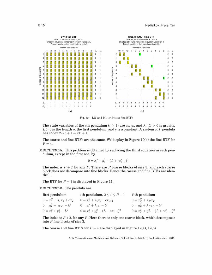
There is no nontrivial block structure, either coarse or fine, as shown in Figure 10(a),for n = 11.
4.1.2. Sparse DAEs. The problems below consist of P chained pendula, where eachpendulum is of size 3. The resulting systems are of size n = 3P , and each pendulum isquasilinear. The aim is to produce parameterized problems of similar sparsity patternsbut differing significantly in index and block structure.
MULTIPEND. The first and the ith pendula (2 ≤ i ≤ P ) arefirst pendulum
0 = x′′1 + λ1x1
0 = y′′1 + λ1y1 −G0 = x21 + y21 − L2
ith pendulum0 = x′′i + λixi
0 = y′′i + λiyi −G0 = x2i + y2i − (L+ cλi−1)2.
ACM Transactions on Mathematical Software, Vol. 41, No. 2, Article B, Publication date: 2015.
B:10 Nedialkov, Pryce, Tan
1 2 3 4 5 6 7 8 9 10 11 12
1
2
3
4
5
6
7
8
9
10
11
12
LW: Fine BTF
Size 12, structural index 1, DOF 1Shaded: structural nonzeros in system Jacobian J
Boxed: positions that contribute to det(J)
0
0
0
0
0
0
0
0
0
0
0
1
0
0
0
0
0
0
0
0
0
0
0
1
0
0
0
0
0
0
0
0
0
0
0
1
0
0
0
0
0
0
0
0
0
0
0
1
0
0
0
0
0
0
0
0
0
0
0
1
0
0
0
0
0
0
0
0
0
0
0
1
0
0
0
0
0
0
0
0
0
0
0
1
0
0
0
0
0
0
0
0
0
0
0
1
0
0
0
0
0
0
0
0
0
0
0
1
0
0
0
0
0
0
0
0
0
0
0
1
0
0
0
0
0
0
0
0
0
0
0
1
0
0
0
0
0
0
0
0
0
0
0
1
0
0
0
0
0
0
0
0
0
0
0
1
0
0
0
0
0
0
0
0
0
0
0
1
0
0
0
0
0
0
0
0
0
0
0
1
0
0
0
0
0
0
0
0
0
0
0
1
0
0
0
0
0
0
0
0
0
0
0
1
0
0
0
0
0
0
0
0
0
0
0
1
0
0
0
0
0
0
0
0
0
0
0
1
0
0
0
0
0
0
0
0
0
0
0
1
0
0
0
0
0
0
0
0
0
0
0
1
0
0
0
0
0
0
0
0
0
0
0
1
0
0
0
0
0
0
0
0
0
0
0
1
0
0
0
0
0
0
0
0
0
0
0
1
1
1
1
1
1
1
1
1
1
1
1
0
c i1
1
1
1
1
1
1
1
1
1
1
0
c i
1 1 1 1 1 1 1 1 1 1 1 1d j
1 1 1 1 1 1 1 1 1 1 1 1d j
Indices of Variables
Ind
ice
s o
f E
qu
atio
ns
(a)
10 11 12 7 8 9 4 5 6 1 2 3
12
11
10
9
8
7
6
5
4
3
2
1
MULTIPEND: Fine BTF
Size 12, structural index 9, DOF 8Shaded: structural nonzeros in system Jacobian J
Boxed: positions that contribute to det(J)
2
0
2
0
0
0
0
2
0
2
0
0
0
0
2
0
2
0
0
0
0
2
0
2
0
0
0
2
0
2
0
0
0
2
0
2
0
0
0
2
0
2
0
0
0
2
0
2
0
0
0
0
0
0 2
0
0
2
0
0
2
0
0
2
0
0
c i2
0
0
4
2
2
6
4
4
8
6
6
c i
2 2 0 2 2 0 2 2 0 2 2 0d j
2 2 0 4 4 2 6 6 4 8 8 6d j
Indices of Variables
Ind
ice
s o
f E
qu
atio
ns
(b)
Fig. 10. LW and MULTIPEND: fine BTFs
The state variables of the ith pendulum (i ≥ 1) are xi, yi, and λi; G > 0 is gravity,L > 0 is the length of the first pendulum, and c is a constant. A system of P pendulahas index 2n/3 + 1 = 2P + 1.
The coarse and fine BTFs are the same. We display in Figure 10(b) the fine BTF forP = 4.
MULTIPENDA. This problem is obtained by replacing the third equation in each pen-dulum, except in the first one, by
0 = x2i + y2i − (L+ cx′i−1)2.
The index is P + 2 for any P . There are P coarse blocks of size 3, and each coarseblock does not decompose into fine blocks. Hence the coarse and fine BTFs are iden-tical.
The BTF for P = 4 is displayed in Figure 11.
MULTIPENDB. The pendula are
first pendulum0 = x′′1 + λ1x1 + cx2
0 = y′′1 + λ1y1 −G0 = x21 + y21 − L2
ith pendulum, 2 ≤ i ≤ P − 1
0 = x′′i + λixi + cxi+1
0 = y′′i + λiyi −G0 = x2i + y2i − (L+ cx′i−1)2
P th pendulum0 = x′′P + λPxP
0 = y′′P + λP yP −G0 = x2P + y2P − (L+ cx′P−1)2
The index is P +2, for any P . Here there is only one coarse block, which decomposesinto P fine blocks of size 3.
The coarse and fine BTFs for P = 4 are displayed in Figure 12(a), 12(b).
ACM Transactions on Mathematical Software, Vol. 41, No. 2, Article B, Publication date: 2015.

DAESA— a MATLAB Tool for Structural Analysis of DAEs: Software B:11
Indices of Variables10 11 12 7 8 9 4 5 6 1 2 3
Ind
ice
s o
f E
qu
atio
ns
12
11
10
9
8
7
6
5
4
3
2
1 2
0
1
2
0
0
0
2
0
1
2
0
0
0
2
0
1
2
0
0
0
2
0
2
0
0
0
2
0
2
0
0
0
2
0
2
0
0
0
2
0
2
0
0
0
2
0
2
0
0
0
1
1
1 2
0
0
2
0
0
2
0
0
2
0
0
ci
2
0
0
3
1
1
4
2
2
5
3
3
ci
2 2 0 2 2 0 2 2 0 2 2 0dj
2 2 0 3 3 1 4 4 2 5 5 3dj
MULTIPENDA: Fine BTF
Size 12, structural index 6, DOF 8Shaded: structural nonzeros in system Jacobian J
Boxed: positions that contribute to det(J)
Fig. 11. MULTIPENDA: coarse and fine BTFs are identical
10 11 12 7 8 9 4 5 6 1 2 3
12
11
10
9
8
7
6
5
4
3
2
1
MULTIPENDB: Coarse BTF
Size 12, structural index 6, DOF 8Shaded: structural nonzeros in system Jacobian J
Boxed: positions that contribute to det(J)
2
0
1
2
0
0
0
0
2
0
1
2
0
0
0
0
2
0
1
2
0
0
0
0
2
0
2
0
0
0
2
0
2
0
0
0
2
0
2
0
0
0
2
0
2
0
0
0
2
0
2
0
0
0
1
1
1 2
0
0
3
1
1
4
2
2
5
3
3
c i
2 2 0 3 3 1 4 4 2 5 5 3d j
Indices of Variables
Indic
es o
f E
quations
(a)
10 11 12 7 8 9 4 5 6 1 2 3
12
11
10
9
8
7
6
5
4
3
2
1
MULTIPENDB: Fine BTF
Size 12, structural index 6, DOF 8Shaded: structural nonzeros in system Jacobian J
Boxed: positions that contribute to det(J)
2
0
1
2
0
0
0
0
2
0
1
2
0
0
0
0
2
0
1
2
0
0
0
0
2
0
2
0
0
0
2
0
2
0
0
0
2
0
2
0
0
0
2
0
2
0
0
0
2
0
2
0
0
0
1
1
1 2
0
0
2
0
0
2
0
0
2
0
0
c i2
0
0
3
1
1
4
2
2
5
3
3
c i
2 2 0 2 2 0 2 2 0 2 2 0d j
2 2 0 3 3 1 4 4 2 5 5 3d j
Indices of Variables
Ind
ice
s o
f E
qu
atio
ns
(b)
Fig. 12. MULTIPENDB: coarse and fine BTFs
MULTIPENDC. We replace the first equation in each pendulum i < P in MULTI-PENDA by
0 = x′′i + λixi + cx′i+1.
The index is P + 2, for any P . There is one coarse block, which does not decomposeinto fine blocks (figure omitted).
ACM Transactions on Mathematical Software, Vol. 41, No. 2, Article B, Publication date: 2015.
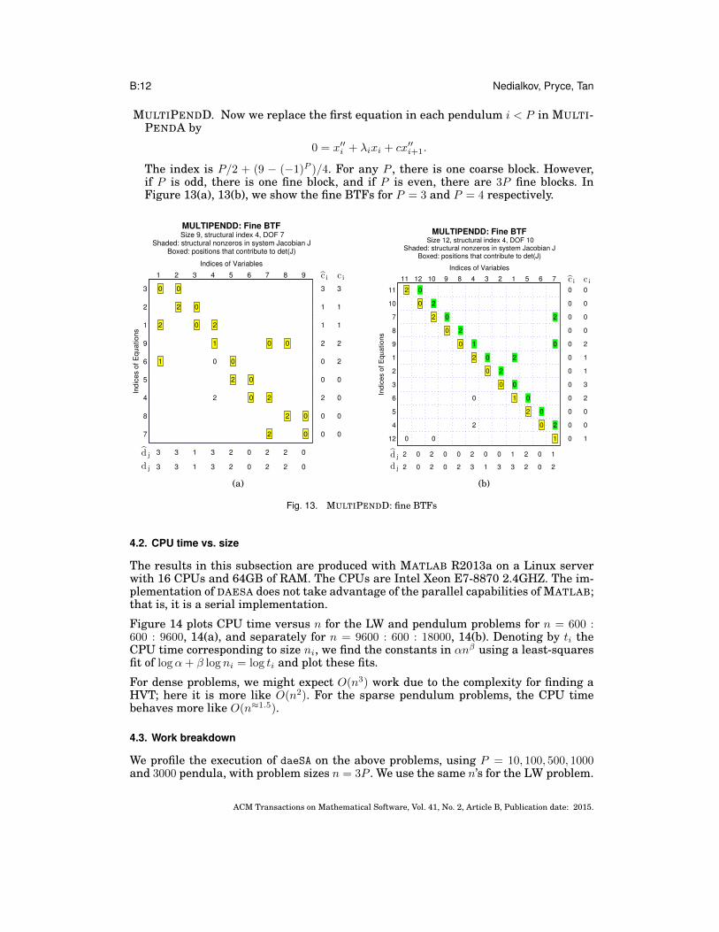
B:12 Nedialkov, Pryce, Tan
MULTIPENDD. Now we replace the first equation in each pendulum i < P in MULTI-PENDA by
0 = x′′i + λixi + cx′′i+1.
The index is P/2 + (9 − (−1)P )/4. For any P , there is one coarse block. However,if P is odd, there is one fine block, and if P is even, there are 3P fine blocks. InFigure 13(a), 13(b), we show the fine BTFs for P = 3 and P = 4 respectively.
1 2 3 4 5 6 7 8 9
3
2
1
9
6
5
4
8
7
MULTIPENDD: Fine BTF
Size 9, structural index 4, DOF 7Shaded: structural nonzeros in system Jacobian J
Boxed: positions that contribute to det(J)
2
0
1
2
0
0
0
2
2
0
1
2
0
0
0
2
2
0
2
0
0
0
2
0
1
2
0
0
0
2
1
2
0
0
0
2
2
0
2
0
0
0
3
1
1
2
0
0
2
0
0
c i3
1
1
2
2
0
0
0
0
c i
3 3 1 3 2 0 2 2 0d j
3 3 1 3 2 0 2 2 0d j
Indices of Variables
Ind
ice
s o
f E
qu
atio
ns
(a)
11 12 10 9 8 4 3 2 1 5 6 7
11
10
7
8
9
1
2
3
6
5
4
12
MULTIPENDD: Fine BTF
Size 12, structural index 4, DOF 10Shaded: structural nonzeros in system Jacobian J
Boxed: positions that contribute to det(J)
2
0
1
2
0
0
0
2
2
0
1
2
0
0
0
2
2
0
1
2
0
0
0
2
2
0
2
0
0
0
1
0
0
2
2
0
1
0
0
2
2
0
2
0
2
0
1
0
0
2
2
0
2
0
2
0 0
0
0
0
0
0
0
0
0
0
0
0
c i0
0
0
0
2
1
1
3
2
0
0
1
c i
2 0 2 0 0 2 0 0 1 2 0 1d j
2 0 2 0 2 3 1 3 3 2 0 2d j
Indices of Variables
Ind
ice
s o
f E
qu
atio
ns
(b)
Fig. 13. MULTIPENDD: fine BTFs
4.2. CPU time vs. size
The results in this subsection are produced with MATLAB R2013a on a Linux serverwith 16 CPUs and 64GB of RAM. The CPUs are Intel Xeon E7-8870 2.4GHZ. The im-plementation of DAESA does not take advantage of the parallel capabilities of MATLAB;that is, it is a serial implementation.
Figure 14 plots CPU time versus n for the LW and pendulum problems for n = 600 :600 : 9600, 14(a), and separately for n = 9600 : 600 : 18000, 14(b). Denoting by ti theCPU time corresponding to size ni, we find the constants in αnβ using a least-squaresfit of logα+ β log ni = log ti and plot these fits.
For dense problems, we might expect O(n3) work due to the complexity for finding aHVT; here it is more like O(n2). For the sparse pendulum problems, the CPU timebehaves more like O(n≈1.5).
4.3. Work breakdown
We profile the execution of daeSA on the above problems, using P = 10, 100, 500, 1000and 3000 pendula, with problem sizes n = 3P . We use the same n’s for the LW problem.
ACM Transactions on Mathematical Software, Vol. 41, No. 2, Article B, Publication date: 2015.
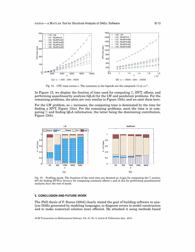
DAESA— a MATLAB Tool for Structural Analysis of DAEs: Software B:13
0 2000 4000 6000 8000 100000
100
200
300
400
500
n
CP
U t
ime
(se
c)
1.78 : LW
1.41 : MultiPend
1.60 : MultiPendA
1.64 : MultiPendB
1.65 : MultiPendC
1.68 : MultiPendD
(a) n = 600 : 600 : 9600
0.8 1 1.2 1.4 1.6 1.8
x 104
0
200
400
600
800
1000
1200
1400
1600
1800
n
CP
U t
ime
(se
c)
1.93 : LW
1.45 : MultiPend
1.37 : MultiPendA
1.53 : MultiPendB
1.54 : MultiPendC
1.49 : MultiPendD
(b) n = 9600 : 600 : 18000
Fig. 14. CPU time versus n. The constants in the legends are the computed β’s in αnβ .
In Figure 15, we display the fraction of time used for computing Σ, HVT, offsets, andperforming quasilinearity analysis (QLA) for the LW and pendulum problems. For theremaining problems, the plots are very similar to Figure 15(b), and we omit them here.
For the LW problem, as n increases, the computing time is dominated by the time forfinding a HVT, Figure 15(a). For the remaining problems, most the time is in com-puting Σ and finding QLA information, the latter being the dominating contribution,Figure 15(b).
(a) (b)
Fig. 15. Profiling daeSA. The fractions of the total time are denoted as: Sigma for computing the Σ matrix;HVT for finding HVT(s); Offsets for computing canonical offsets c and d; QLA for performing quasilinearityanalysis; Rest the rest of daeSA.
5. CONCLUSION AND FUTURE WORK
The PhD thesis of P. Bunus [2004] clearly stated the goal of building software to ana-lyze DAEs generated by modeling languages, to diagnose errors in model constructionand to make numerical solution more efficient. He attacked it using methods based
ACM Transactions on Mathematical Software, Vol. 41, No. 2, Article B, Publication date: 2015.
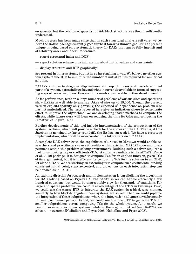
B:14 Nedialkov, Pryce, Tan
on sparsity, but the relation of sparsity to DAE block structure was then insufficientlyunderstood.
Much progress has been made since then in such structural analysis software; we be-lieve the DAESA package currently goes furthest towards Bunus’s goal. It is at presentunique in being based on a systematic theory for DAEs that can be fully implicit andof arbitrary order and index. Its features:
— report structural index and DOF;
— report solution scheme plus information about initial values and constraints;
— display structure and BTF graphically;
are present in other systems, but not in so far-reaching a way. We believe no other sys-tem exploits fine BTF to minimize the number of initial values required for numericalsolution.
DAESA’s abilities to diagnose ill-posedness, and report under- and over-determinedparts of a system, potentially go beyond what is currently available in terms of suggest-ing ways of correcting them. However, this needs considerable further development.
As for performance, tests on a large number of problems of various sizes and sparsitiesshow DAESA is well able to analyze DAEs of size up to 18,000. Though the currentversion exploits sparsity only partially, the expected n3 dependence on problem sizehas not materialized. The tests reported here give an indication where to concentrateeffort to improve the algorithms. We are developing faster methods to compute theoffsets, while future work will focus on reducing the time for QLA and computing theΣ matrix; cf. Figure 15(b).
Further developments of this tool include implementation of the computation of thesystem Jacobian, which will provide a check for the success of the SA. That is, if thisJacobian is nonsingular (up to roundoff), the SA has succeeded. We have a prototypeimplementation, which will be incorporated in a future version of DAESA.
A complete DAE solver (with the capabilities of DAETS) in MATLAB would enable re-searchers and practitioners to use it readily within existing MATLAB code and to ex-periment within this problem-solving environment. Building such a solver requires atool for computing Taylor coefficients (TCs). A suitable candidate is the ADTAYL [Pryceet al. 2010] package. It is designed to compute TCs for an explicit function, given TCsof its argument(s), but it is inefficient for computing TCs for the solution to an ODE,let alone a DAE. We are working on extending it to compute such coefficients. Findingconsistent initial point, stepsize control, and projections on each integration step canbe handled as in DAETS.
An exciting direction for research and implementation is parallelizing the algorithmsfor DAE solving based on Pryce’s SA. The DAETS solver can handle efficiently a fewhundred equations, but would be unacceptably slow for thousands of equations. Forlarge and sparse problems, one could take advantage of the BTFs in two ways. First,we could use the coarse BTF to integrate the DAE system in a block-wise manner,similarly to how block-triangular linear systems are solved. Then we could pipelinethe integration of these subproblems, where the integrations advance asynchronouslyin time (companion paper). Second, we could use the fine BTF to generate TCs forsmaller subproblems, versus computing TCs for the whole system. As a result, weneed to solve smaller linear systems, while in the original method (and DAETS), wesolve n× n systems [Nedialkov and Pryce 2005; Nedialkov and Pryce 2008].
ACM Transactions on Mathematical Software, Vol. 41, No. 2, Article B, Publication date: 2015.

DAESA— a MATLAB Tool for Structural Analysis of DAEs: Software B:15
In its present form, DAESA is a collection of MATLAB functions, so that its facilitiesare invoked at the MATLAB command line or within code. We are developing a GUIinterface to DAESA that will allow interactive study of DAEs. This will allow zoominginto the structure of large matrices and identifying lines of code that lead to a givenpattern in the signature or system Jacobian matrix.
ACKNOWLEDGMENTS
The authors are grateful to Ian Washington from the Department of Chemical Engineering of McMasterUniversity for numerous discussions and suggestions on improving DAESA, providing DAE problems andencoding them in DAESA, and in particular the model in §3.2.
We acknowledge with thanks the support given to JDP by the Leverhulme Trust and the Engineering andPhysical Sciences Research Council, both of the UK, and to GT and NSN by the Canadian Natural Sciencesand Engineering Research Council and the McMaster Centre for Software Certification.
REFERENCES
BRENAN, K., CAMPBELL, S., AND PETZOLD, L. 1996. Numerical Solution of Initial-Value Problems inDifferential-Algebraic Equations second Ed. SIAM, Philadelphia.
BUNUS, P. 2004. Debugging techniques for equation-based languages. Ph.D. thesis, Linkoping University,Sweden, Department of Computer and Information Science.
DAVIS, T. A. AND HU, Y. 2011. The University of Florida sparse matrix collection. ACM Trans. Math.Softw. 38, 1, 1:1–1:25.
HINDMARSH, A. C., BROWN, P. N., GRANT, K. E., LEE, S. L., SERBAN, R., SHUMAKER, D. E., AND WOOD-WARD, C. S. 2005. SUNDIALS, Suite of Nonlinear and Differential/Algebraic Equation Solvers. ACMTrans. Math. Softw. 31, 3, 363–396.
MATTSSON, S. E. AND SODERLIND, G. 1993. Index reduction in differential-algebraic equations usingdummy derivatives. SIAM J. Sci. Comput. 14, 3, 677–692.
MAZZIA, F. AND IAVERNARO, F. 2003. Test set for initial value problem solvers. Tech. Rep. 40, Departmentof Mathematics, University of Bari, Italy. http://pitagora.dm.uniba.it/~testset/.
MCKENZIE, R., NEDIALKOV, N. S., PRYCE, J., AND TAN, G. 2013. DAESA user guide. Tech. rep., De-partment of Computing and Software, McMaster University, Hamilton, Ontario, Canada, L8S 4K1.http://www.cas.mcmaster.ca/~nedialk/daesa/daesaUserGuide.pdf.
NEDIALKOV, N. AND PRYCE, J. 2008–2009. DAETS user guide. Tech. rep., Department of Computing andSoftware, McMaster University, Hamilton, Ontario, Canada, L8S 4K1.
NEDIALKOV, N. S. AND PRYCE, J. D. 2005. Solving differential-algebraic equations by Taylor series (I):Computing Taylor coefficients. BIT 45, 561–591.
NEDIALKOV, N. S. AND PRYCE, J. D. 2007. Solving differential-algebraic equations by Taylor series (II):Computing the System Jacobian. BIT 47, 1, 121–135.
NEDIALKOV, N. S. AND PRYCE, J. D. 2008. Solving differential-algebraic equations by Taylor series (III):The DAETS code. JNAIAM 3, 1–2, 61–80. ISSN 17908140.
PRYCE, J., GHAZIANI, R. K., WITTE, V. D., AND GOVAERTS, W. 2010. Computation of normal form co-efficients of cycle bifurcations of maps by algorithmic differentiation. Mathematics and Computers inSimulation 81, 1, 109 – 119.
J. D. PRYCE, N. S. NEDIALKOV, AND G. TAN, DAESA: a Matlab tool for structural analysis of differential-algebraic equations: Theory, ACM Trans. Math. Softw., 41 (2015), pp. 9:1–9:20.
PRYCE, J. D. 2001. A simple structural analysis method for DAEs. BIT 41, 2, 364–394.WASHINGTON, I. AND SWARTZ, C. 2011. On the numerical robustness of differential-algebraic distillation
models. In 61st Canadian Chemical Engineering Conference. London, Ontario, Canada.WATSON, L. T. 1979. A globally convergent algorithm for computing fixed points of C2 maps. Appl. Math.
Comput. 5, 297–311.
ACM Transactions on Mathematical Software, Vol. 41, No. 2, Article B, Publication date: 2015.