H e l i S n e l l m a n

Automated Teller Machinenetwork market structure and cash usage

S c i e n t i f i c m o n o g r a p h s

E : 3 8 · 2 0 0 6

The views expressed in this study are those of the author and do not necessarily reflect the views of the Bank of Finland.

ISBN 952-462-318-8ISSN 1238-1691(print)

ISBN 952-462-319-6ISSN 1456-5951(online)

Edita Prima OyHelsinki 2006

3

Abstract This study discusses the effects of the Automated Teller Machine (ATM) network market structure on the availability of cash withdrawal ATM services and cash usage. The aim and novelty of the study is to construct the ATM equation. The study also contributes to the earlier discussion on the effects of ATMs on cash usage. The monopolisation of ATM network market structure and its effects on the number of ATMs and on cash in circulation are analysed both theoretically and empirically. The unique annual data set on 20 countries used in the estimations has been combined from various data sources. The observation period is 1988–2003, but the data on some countries are available only for a shorter period. Based on our theoretical discussion, as well as the estimation results, monopolisation of the ATM network market structure is associated with a smaller number of ATMs. Furthermore, the influence of the number of ATMs on cash in circulation is ambiguous. Key words: ATM, ATM network, monopolisation, demand for cash JEL classification: C33, E41, G2, C11

4

Tiivistelmä Tässä tutkimuksessa tarkastellaan käteisautomaattiverkkojen mark-kinarakenteen vaikutuksia automaattipalvelujen saatavuuteen ja kätei-sen käyttöön. Työn tarkoituksena on luoda automaattien määrää ku-vaava yhtälö sekä osallistua aiempaan keskusteluun automaattien vai-kutuksista kierrossa olevan käteisen määrään. Automaattiverkkojen markkinarakenteen monopolisoitumisen vaikutusta automaattien mää-rään ja kierrossa olevan käteisen arvoon analysoidaan sekä teoreetti-sesti että empiirisesti. Estimoinneissa käytetään laajaa, eri lähteistä koottua 20 maan vuosiaineistoa. Tarkasteluperiodi on 1988–2003, mutta joillekin maille dataa on saatavilla lyhyemmälle periodille. Saatujen tulosten perusteella automaattiverkkojen markkinarakenteen monopolisoituminen vähentää automaatteja, mutta automaattien vai-kutus kierrossa olevan käteisen arvoon on epäselvä. Avainsanat: käteisautomaatti, automaattiverkko, monopolisoituminen, käteisen kysyntä JEL-luokittelu: C33, E41, G2, C11

5

Acknowledgements This study was written mostly during my stay at the Research Unit of the Bank of Finland and was accepted in spring 2006 as my licentiate thesis for the Helsinki School of Economics. I am grateful to Jouko Vilmunen, Matti Virén, Karlo Kauko, Juha Tarkka and Antti Kanto for their advice and invaluable comments in the course of the project. Furthermore, I wish to thank Emmi Martikainen for her help with data collection and Päivi Nietosvaara for her help with editorial work. I would also like to thank Glenn Harma for improving the language of the study, as well as Heikki Koskenkylä and Kari Korhonen for the opportunity to finalise the study in the Financial Markets and Statistics Department of the Bank of Finland. Finally, I am grateful to my family and friends, and especially to my husband Jussi, for their support and patience throughout the project. Helsinki, July 2006 Heli Snellman

7

Contents Abstract...............................................................................................3 Tiivistelmä...........................................................................................4 Acknowledgements.............................................................................5 1 Introduction ...................................................................................9 2 Literature review.........................................................................13 2.1 Literature on ATMs................................................................13 2.2 Survey on money demand ......................................................17 2.2.1 Macro-economic and micro-economic levels of money demand.......................................................17 2.2.2 Transactions demand for currency and other payment instruments .........................................18 2.2.3 Effects of ATMs on money demand...........................20 2.3 Monopolisation ......................................................................22 2.4 Network externalities: compatibility and threat of entry ........23 2.5 Pricing structure and fees .......................................................26 2.6 Contribution to the existing literature.....................................27 3 Two alternative models ...............................................................29 3.1 Spatial model..........................................................................29 3.1.1 The consumer’s decision ............................................30 3.1.2 The bank’s decisions ..................................................34 3.2 Transaction-size model ..........................................................40 3.2.1 The consumer’s decisions ..........................................40 3.3 Comparison between spatial and transaction-size models......42 3.4 Implications for empirical work .............................................45 4 Empirical evidence ......................................................................47 4.1 Data description .....................................................................47 4.1.1 Availability of data.....................................................52 4.2 Equations to be estimated.......................................................53 4.2.1 Dynamic model specifications ...................................53 4.2.2 ATM equation ............................................................55 4.2.3 Cash equation .............................................................58 4.3 Estimation results ...................................................................60 4.3.1 Choice of estimation method......................................60 4.3.2 Results of ATM equation estimations ........................61 4.3.3 Results of cash equation estimations ..........................66 4.4 Discussion of estimation results .............................................69

8

5 Conclusions ..................................................................................73 5.1 Policy discussion....................................................................74 5.2 Topics for further research .....................................................76 References .........................................................................................77 Data sources......................................................................................90 Appendix 1 Profit maximisation in the competitive case.................92 Appendix 2 ATM network market structure in each country...........94 Appendix 3 Variable figures..........................................................100 Appendix 4 Unit root tests .............................................................104 Appendix 5 Symbols and abbreviations.........................................105

9

1 Introduction Payment systems have developed rapidly in many countries over the past few decades. The use of electronic means of payment has increased at the expense of paper-based payment instruments. For instance, in some countries payment cards have replaced cheques, and Internet banking has become a popular means of paying invoices. The developments in payment systems and especially in cash usage are very important for central banks. Central banks ought to promote stable, reliable and efficient payment systems. Furthermore, the maintenance of currency supply is one of the main responsibilities of central banks. Cash is the only legal tender, and cash issuance is a central bank monopoly and the basis of seigniorage for central banks. Maintenance of the currency supply includes distribution of notes and coins to end-users. Automated Teller Machines (ATMs1) are nowadays a very common technology for dispensing notes to cash-holders. Putting notes into circulation via ATMs involves two main parties: the central bank and banks, or bank-owned companies, which typically maintain ATMs and ATM networks2. The interests of these two parties may be somewhat conflicting: from the central bank’s point of view, increased cash usage is good, as it generates seigniorage; whereas for banks less cash usage is preferable since cash usage entails costs to banks but hardly any income. Therefore, it may be in banks’ interests to reduce cash usage and the number of ATMs. In addition to central banks and banks, cash usage has relevance for consumers, as well. Consumers decide, based on financial and inconvenience costs, whether to pay for transactions with cash or some other payment instrument. How do cash dispensing technology choices or changes in this technology affect cash usage and maintenance of the currency supply? What happens if banks decide to radically reduce the number of ATMs? Do people hold less cash because it is difficult to find an ATM and withdraw cash? Or do people hold more cash because they

1 By ATM (Automated Teller Machine) we mean a machine at which a customer can withdraw cash. Typically, these machines also provide other functions, eg reporting the balance on a customer’s account. There are also machines that are used for making credit transfers or deposits. In this study, we concentrate particularly on cash withdrawal ATMs and use the terms cash dispenser, ATM and cash-withdrawal ATM as synonyms. 2 The ATMs of a bank, banking group or other credit institution constitute an ATM network. It is possible that ATM networks are interoperable, ie compatible, with each other. Compatible networks are sometimes called shared networks.

10

withdraw greater amounts of cash as visiting ATMs becomes more inconvenient? Based on the earlier literature, eg Boeschoten (1992, 1998), Snellman et al (2000), Drehmann and Goodhart (2000) and Drehmann et al (2002), the effects of ATMs on cash in circulation are somewhat ambiguous. Also, the reduction in the number of ATM networks may reduce the number of ATMs and affect the demand for cash. Furthermore, the effects of ATM network market structure on cash usage may also depend on other payment instruments. If there are convenient and inexpensive payment instruments available, changes in ATM network market structure may have greater effects on cash usage than in infrastructures where cash is the only payment instrument available. The market structure of cash withdrawal ATM networks differs across countries. Even in the euro area, there are countries with only one ATM network and other countries with many. There have also been changes in the ATM network market structure during the past fifteen years in many countries. Finland is a good example of this. Until 1994, each bank had its own ATM network, and these had been compatible for some years. In 1994, the biggest banks3 decided to close down their own networks. They founded a jointly owned company, called Automatia Pankkiautomaatit Ltd. This company, which bought the ATMs of the owner banks and the ATMs of Suomen Säästöpankki, established a common ATM network (Otto.network), and began to maintain the ATMs in it. In addition to this network, there were two considerably smaller cash withdrawal ATM networks in Finland in 1994–2004. All three of these networks were compatible, but during the later years customers had to pay a fee for using rival banks’ ATMs. In 2004, the small banks decided to close down their two networks and to start using Otto.network. Otto.ATMs are still owned by Automatia Pankkiautomaatit Ltd, and all banks are customers of this network. Customers of all banks are generally able to withdraw cash free of charge. In Finland, reductions in ATM networks have always resulted in reductions in the number of ATMs. For instance, at the start of the 1990s, the number of ATMs decreased by 14.5% in one year as ATMs were closed in connection with the merger of ATM networks. Before the merger, banks were competing fiercely with each other, and one way to do this was to provide ATM services at their own ATMs. In fact, Finland is the only country where the number of ATMs has decreased considerably. The number of ATMs decreased continually

3 KOP, SYP, Osuuspankki and Postipankki.

11

during 1993–2003, dropping from 2994 to 2421 in 1993–1995 alone. Thus, monopolisation of the ATM network market structure seems to have reduced the number of ATMs. On the other hand, at the start of the 1990s, there was a severe banking crisis in Finland, which forced banks to cut costs. However, the banking crisis cannot be the only reason behind the reduction in ATMs. As stated above, the two small networks were closed down in 2004. As a result, ca 300 ATMs were closed and, at the same time, ca 80 new Otto.ATMs were installed. On this occasion, the reduction of ATMs could hardly have been the consequence of the banking crisis. In other words, monopolisation again led to fewer ATMs. In other countries, however, the tendency towards fewer ATMs has not been as pronounced as in Finland. Therefore, the monopolisation effects on the number of ATMs should be studied more closely. We describe developments and differences across countries in detail in Section 4.1 and Appendix 2. The monopolisation of ATM networks and its effects on the number of ATMs and cash usage have not been widely discussed in the literature. The aim of this study is to highlight these aspects. The novelty of the study is to construct an ATM equation which depends on the number of ATM networks. We analyse the influence of monopolisation of the ATM network market structure both theoretically and empirically. A further aim is to contribute to the earlier discussion on the effects of the number of ATMs on cash usage. This question has been analysed in many earlier studies, but with mixed results: According to some studies, cash usage depends positively on the number of ATMs, whereas some other studies indicate the opposite result. Because of the ambiguous results in the earlier literature, we contribute to this discussion with both our theoretical and empirical analysis. We concentrate on the question of how ATMs affect cash usage when there is another payment technology available. Moreover, the earlier discussion on the demand for money and alternative payment instruments typically concentrates on the consumer side, ie the demand side. The bank (supply) side is also important because banks maximise profits and decide on the number of ATMs. In this analysis, the bank’s behaviour and the profit function behind its decisions are highlighted. Furthermore, we concentrate mostly on the transactions demand for cash and assume that all cash is withdrawn at ATMs. In reality, the importance of

12

ATMs as a cash distribution channel differs across countries. Some cash is withdrawn eg at bank branches or at EFTPOS4. To sum up, we analyse, theoretically and empirically, two research questions: 1) how do changes in the ATM network market structure affect the number of ATMs and 2) how does this affect cash usage. We use in our estimations a unique data set on 20 countries for the period 1988–2003. The structure of the report is as follows. In Section 2, we present a review of the literature. Next, we discuss the factors that determine a consumer’s cash usage and a bank’s provision of ATM services. We formalise this discussion theoretically in Section 3. Section 4 provides the relevant empirical evidence: the data, estimation results and main findings of the estimations. Section 5 concludes the study, and includes some policy discussion and possible future research topics.

4 EFTPOS refers to electronic fund transfer point-of-sale, ie a machine in a shop at which consumers pay with their payment cards.

13

2 Literature review This section first summarises earlier ATM studies. Recent discussion on ATMs has concentrated on the pricing structure and fees for ATM services. Network externalities of ATMs, as well as cost savings, have also been studied. The discussion has included technology adoption and used ATMs as an example of diffusion. The ATM discussion indicates that monopolisation of the ATM network market structure has not been widely analysed. Furthermore, this section briefly discusses the development of the theory of money demand, focusing on the transactions demand for money. The reason for this focus is that ATMs may have some influence on money demand, and one purpose of our study is to contribute to this discussion. The effects of monopolisation that are analysed in the industrial organisation literature are also briefly discussed here, since we study the effects of ATM network monopolisation on the availability of ATM services and cash in circulation. We also discuss compatibility and entry into markets with network externalities because these may be important in ATM networks. In addition, some papers on pricing and costs of payment instruments and payment systems are presented, as pricing and fee structures have recently been discussed widely in the payment systems literature. 2.1 Literature on ATMs

ATMs have been analysed in the literature for some thirty years. The earliest studies concentrate on explaining the adoption of this new technology. Mandell (1977) discusses ATM adoption in the USA. The first ATM was installed in the USA in 1969 and, according to Mandell, only 10% of all national banks had adopted even one ATM after eight years. Mandell states that a bank’s adoption of innovation depends eg on its size, branching status and competitive position. According to Mandell, in those days adoption of new technology was related more closely to competition than to cost savings. Hannan and McDowell (1987) examine how firms react to rivals’ precedence in technology adoption process. The authors use data on the adoption of ATMs by a large sample of US banking firms in 1971–1979. According to the study, rivals’ adoption of ATMs increases the conditional probability that the other firms will also adopt ATMs. Hannan and McDowell (1984a and 1984b) state that market

14

concentration has positive effects on the adoption of ATMs. Saloner and Shepard (1995) study empirically the adoption of ATMs in the USA in 1972–1979. According to their results, ATM adoption delays are reduced as network effects increase. The authors use the number of branches as a proxy for network effects because, in the 1970s, most ATMs were located in bank branches. However, today such a proxy would not be appropriate because many ATMs are located outside of banking premises. Furthermore, the authors state that ATMs are adopted the sooner, the greater the production scale economies. McAndrews and Kauffman (1993) discuss network externalities and shared ATM networks. According to this study, the number of bank’s own branches is not related to early ATM adoption but the number of other banks’ branches is. Frame and White (2004) survey ATM diffusion studies in their article on empirical studies of financial innovation. The six studies summarised by Frame and White discuss initial adoption, or diffusion, of ATM technology. However, the demand for ATMs after the first phase of adoption has not been discussed very widely. Hester et al (1999) study decisions on ATMs in Italian banks. According to their results, the number of ATMs is positively related eg to the bank’s number of branches and deposit accounts. There are studies on ATM pricing and fees. There are various fees related to ATMs: An interchange fee is a fee that the customer’s bank pays to the ATM owner when the customer uses another bank’s ATM. A surcharge fee is paid by the cardholder to the ATM owner. A foreign fee is paid by the cardholder to his bank when using another bank’s ATM. These and other fee definitions are found in McAndrews (2003). Salop (1990) discusses the pricing decisions of shared ATM networks. He states that ATM networks should eliminate their pricing rules for interchange fees and that there should be price competition between ATM owners in order to increase the efficiency. Matutes and Padilla (1994) investigate shared ATM networks, banking competition and fees. The authors use a three-bank model to study the manner in which banks make their ATM networks compatible. They conclude that in equilibrium either a subset of banks will share ATM networks or there will be total incompatibility. This is a somewhat surprising result, since many national ATM networks seem to be compatible (eg ECB 2001). On the other hand, there have been changes in compatibility during the 1990s. The paper was published in 1994, when incompatibility was more typical than nowadays. According to Matutes and Padilla (1994), fully compatible networks are found in countries where the banking system is highly collusive, dominated by

15

public banks, or competing in different geographical markets. Furthermore, Matutes and Padilla state that network fees enhance the likelihood of compatibility. Hannan et al (2003) analyse the pricing of ATM usage and surcharge levels in the USA. This empirical paper studies depository institutions’ decisions on whether to have surcharges on non-depositors using their ATMs. The authors conclude that the probability of surcharging is positively related to the institution’s share of ATMs and negatively related to local ATM density. Massoud and Bernhardt (2002) investigate theoretically the pricing of ATM services. According to their results, in equilibrium, banks charge non-member users high ATM fees but do not charge their own customers for ATM usage. Own customers have to pay high bank account fees, and larger banks charge higher bank account fees and higher surcharges than smaller banks. The authors state that forcing banks to charge both members and non-members the same ATM fees leads to higher ATM prices and bank profits, and possibly to less consumer welfare. Partly based on Massoud and Bernhardt (2002), Massoud et al (2003) analyse empirically ATM surcharges and customer relationships. They find that changes in ATM surcharges have a direct effect on bank profitability and an indirect effect via customer switching to use of other services provided by the bank. Prager (2001) analyses the effects of ATM surcharges on small banks, comparing states that allowed surcharging prior to 1995 and those that did not. Contrary to the results by Massoud et al (2003), Prager (2001) finds that ATM surcharges do not affect banks’ profitability. Also Croft and Spencer (2003) analyse fees and surcharging in ATM networks. They develop a theoretical model and conclude that surcharging raises the customer’s price above the joint profit-maximising level for a shared network. Joint profits of the shared network are maximised by setting the interchange fee at marginal cost and not surcharging. Furthermore, large banks prefer lower interchange fees than do small banks. McAndrews (1992) discusses ATM network pricing based on a survey conducted in 1989 and 1990 in the USA. McAndrews (1998) discusses ATM surcharges in the USA, and McAndrews (2003) reviews the ATM pricing literature. There is very little discussion on competition, mergers or monopolisation of ATM networks. McAndrews and Rob (1996) compare theoretically competition between two solely owned switches (ATM networks) and between one solely owned and one jointly owned switch. The authors study these two duopolies and differences in supplied quantities and profits, assuming the existence of network

16

externalities in the ATM market. According to their results, the equilibrium profits of banks in the solely owned network are the same in both duopoly cases. On the other hand, the equilibrium profits of banks in the jointly owned network are higher than the equilibrium profits of banks in the solely owned network in the case of one solely owned and one jointly owned network. In addition to the equilibrium profits from supplying ATM services to customers, banks in the jointly owned network receive part of the profits of the jointly owned network. Furthermore, the authors state that the network jointly owned by all banks produces the monopoly output, and consumers pay the monopoly price. They also discuss welfare implications and conclude that, because of network externalities and economies of scale, the monopoly may be a better structure in the end. Carlton and Frankel (1995) discuss the merger between two ATM networks in Chicago. These two networks, Cash Station and Money Network, were competitors until 1987. After the merger decision and a transition period, all ATM terminals of the new-combined network were available to all customers in early 1988. Carlton and Frankel state, on the basis of the statistics, that the growth in the number of ATMs in the new network has been faster than average growth in the number of ATMs in the USA. Furthermore, the volume of transactions increased even though the interchange fee of the new network was increased in 1991. Based on these arguments, the authors state that the merger of these two ATM networks benefited consumers. Also Balto (1995) and Baker (1995) discuss mergers of ATM networks in the USA. They are clearly more skeptical about the benefits of ATM network mergers than Carlton and Frankel (1995). Horvitz (1996) discusses the effects of ATM surcharges on competition and efficiency. According to Horvitz, the Department of Justice and the Federal Reserve failed to prevent the consolidation of ATM networks in the USA in the 1980s. He presumes that high surcharges charged by large banks will encourage small banks to provide ATM networks at lower costs or even without surcharges, which may restore competition in the ATM network market. Cost savings from ATMs and electronic payments have also been discussed. Humphrey (1994) studies possible cost savings and concludes that ATMs have not reduced banks’ costs. This may be the case because consumers use ATM services more intensively than services provided in bank branches. However, Humphrey et al (2003a) get the opposite results. They analyse cost savings from ATMs and electronic payments in 12 European countries in 1987–1999. According to the results, the ratio of operating costs of providing banking services to total assets has decreased considerably because of

17

electronic payments and use of ATMs. Humphrey et al (2003b) and Humphrey and Vale (2004) state that the shift to electronic-based payments leads to remarkable cost savings. In addition, Humphrey and Vale (2004) discuss cost savings from bank mergers. They use Norwegian banking sector data and state that bank mergers in Norway have on average reduced costs. Hancock et al (1999) discuss the consolidation of Fedwire and find that consolidation reduced costs. Humphrey et al (1998) investigate the gains from electronic payments with Norwegian data and conclude that electronic payments lead to social benefits. Raa and Shestalova (2004) analyse payment media costs with Dutch data and find that currency is cost-effective for small payments. Furthermore, their results suggest that debit cards or e-money are likely to replace cash usage for larger legal transactions. To conclude, various aspects of ATMs have been analysed in the literature. The earliest ATM papers concentrated on the adoption of ATMs, and a significant part of the recent literature discussed the pricing and cost saving questions. However, the effects of monopolisation in the ATM network market structure have attracted insufficient attention. Our analysis is aimed to fill this gap in the literature. 2.2 Survey on money demand

In this section, we briefly review money demand theory. After a general overview, we concentrate on the transactions demand for currency. 2.2.1 Macro-economic and micro-economic levels of

money demand

One way to approach the money demand literature is to divide it into macro-economic and micro-economic levels. The development of money demand theory discussed in this sub-section are based on Boeschoten (1992, ch. 1) and Tarkka (1993, ch. 6). More detailed analyses, discussion and references are found in these two books. Fisher’s (1911)5 quantity theory focuses on money as a means of exchange. The basic idea is encapsulated in the famous equation of

5 Fisher (1911): The Purchasing Power of Money (in Tarkka 1993).

18

exchange, MV = PT, where M is the stock of money, V the circulation velocity of money, P the price level and T the volume of total transactions. The cash balance approach of Pigou and Marshall is another version of the quantity theory, which is also referred to as the Cambridge approach. Pigou (1917)6 expressed this approach as M = kPY, where M is the stock of money, P the price level, Y real income and k a constant (Cambridge k). Keynes (1936)7 emphasised the importance of the interest rate, and one of his central assumptions was that money demand depends negatively on the interest rate level. In the 1950s, Friedman8 began to criticise the Keynes approach, and interest in the quantity theory increased. The application of the portfolio approach to economic theory presented by Tobin (1958) analyses money holdings as part of a portfolio. In this approach, the demand for money depends on the risk of other assets and on the rates of return. The micro-economic theory of money demand can be divided in three categories: the transactions demand, the precautionary demand and the speculative demand. Transactions demand means the need for money to pay for transactions. Precautionary demand means that some part of cash balances is held for sudden and surprising purchases. The speculative demand for money is related to uncertainties as to the returns on other forms of people’s wealth: money holdings may be held because the risk is low, whereas other forms of wealth may entail uncertainty eg about interest rates and capital losses. The speculative demand for cash may be highlighted eg in developing countries or in countries where people do not rely on the banking sector. The precautionary and speculative demands for cash are not discussed in detail in this study. 2.2.2 Transactions demand for currency and other

payment instruments

Baumol (1952) discusses the transactions demand for cash. According to this model, the demand for cash depends on the value of transactions, cost of withdrawing cash and interest opportunity cost. Tobin (1956) discusses the interest elasticity of the transactions

6 In Boeschoten 1992. 7 Keynes (1936) A General Theory of Employment, Interest, and Money (in Tarkka 1993). 8 Friedman (1956); in Boeshoten 1992.

19

demand for cash. Romer (1986) presents a general equilibrium version of the Baumol-Tobin model, in which money is both the store of value and the medium of exchange, and the consumer’s cash holdings depend on the inconvenience of trips to the bank and interest rate losses from holding cash instead of higher-yield assets. Santomero (1979) analyses the demand for currency and for deposits. The average deposit balance depends eg on the fraction of total transactions paid by cash, the expenditure, the rate of return on the deposit account, the costs of transfer from the interest-bearing asset, and the cost of purchasing the commodity with demand deposits. Santomero and Seater (1996) discuss the demand for media of exchange when there is an arbitrary number of payment instruments available. They analyse a representative agent model and state that the range of asset use decreases as household income decreases. Furthermore, the usage of payment instrument depends on the consumption patterns. Whitesell (1989) analyses the demand for currency and the demand for debitable accounts drawn on by check, debit card or credit card. In this model, the consumer makes purchases of various sizes, and the size of the transaction determines the means of payment used. The smallest transactions are paid in cash while transactions that exceed λ are paid with other means of payment. Whitesell (1992) analyses optimal service fees and deposit interest rates set by banks. Whitesell includes in his model currency, checks and credit cards, and discusses equilibrium under a monopoly bank and competitive banks. Shy and Tarkka (2002) study the use of electronic cash cards, charge cards and currency. They analyse the costs of these three means of payment for both merchant and consumer sides. According to the results of this theoretical paper, in the absence of fees the smallest purchases are paid by electronic cash card, mid-size purchases in currency and the largest purchases by charge card. Another approach is to assume that the commodity itself determines which transactions are paid in cash and which transactions by card. In other words, some commodities must be paid in cash and some by credit. For instance, Lucas and Stokey (1987) analyse the use of money with an aggregate general equilibrium model, assuming that there are two consumption goods – cash goods and credit goods – available each period. Lucas and Stokey state that one way to interpret credit goods is to define them as non-market goods, such as leisure. White (1976) analyses the effects of credit cards on households’ demand for money. He states that increased use of credit cards can be expected to reduce the amount of money needed for transactions. Duca and Whitesell (1995) also discuss the effects of credit cards on

20

household money demand. According to their results, credit card ownership is negatively related to transaction deposits. Markose and Loke (2003) discuss network effects on cash-card substitution. They state that there is a unique relationship between EFTPOS coverage and the proportion of cash financed expenditures in equilibrium. Mulligan (1997) analyses the use of cash by firms and finds that large firms hold less cash than small firms, relative to sales. Similar results are found by Hirvonen and Virén (1996a, 1996b), who use survey data on Finnish business firms and find that the ratio of cash payments to total sales is considerably higher for small firms than for large firms. Humphrey et al (1996) empirically study the use of cash and five non-cash payment instruments (check, paper giro, electronic giro, credit card and debit card). They use data on 14 countries for 1987–1993 and conclude that countries generally move to increased use of electronic payment methods even when the mix of payment instruments differs considerably across countries. Avery (1996) comments on the study of Humphrey et al (1996) and emphasises that the exogenous variables that cause the differences between payment systems are not self-evident. Judson and Porter (2004) analyse currency demand in the USA in 1974–1998. They find that currency demand depends eg on transactions, income, age distribution, bankruptcies, crime, employment, transfer payments and international currency demand. Virén (1993, 1994) discusses the demand for different payment instruments in Finland based on survey data. Mulligan and Sala-i-Martin (1996, 2000) study the adoption of financial technologies. They state that the relevant question is whether people hold interest-bearing assets, not the fraction of such assets. The main factor behind the choice is the product of interest rate times the total amount of assets. Angelini et al (1994) analyse money demand in Italy. They find that money demand was unstable in the early 1980s because new instruments for Treasury funding were launched. They note that people began to use new instruments, and the demand for money as a store of value declined. Rinaldi and Tedeschi (1996) discuss money demand in Italy using a system approach. Duca and VanHoose (2004) summarise a segment of the literature on money demand. 2.2.3 Effects of ATMs on money demand

Paroush and Ruthenberg (1986) discuss the effects of ATMs on the share of demand deposits in the money supply. The authors use Israeli data and find that the introduction of ATMs increases deposits at the

21

expense of currency holdings. Boeschoten (1992, p. 192) also discusses the influence of ATMs on cash demand. According to this study, ATMs have a positive effect on the nominal currency growth, but this effect is not very robust. Boeschoten (1998) continues the discussion about ATM influence on cash demand with Dutch data in 1990–1994. He finds that ATMs lead to reduced cash demand by the public but increased inventories of currency held by the banking sector for ATM usage. Thus the total effect of ATMs on the total amount of currency outstanding is quite moderate. Hancock and Humphrey (1998) discuss the influence of ATMs on cash holdings and conclude that the effects are somewhat mixed. Snellman et al (2000) study the effects of ATMs on cash demand with data on 10 European countries for 1987–1996. According to their results, there is a negative relationship between ATM usage and cash balances, ie ATMs have reduced the public’s demand for cash balances. Attanasio et al (2002) analyse the demand for currency with household data from Italy and find that the diffusion of ATM cards is the main factor explaining the decrease in currency demand. The currency-consumption ratio is considerably higher for households with no bank account or ATM card. Furthermore, the demand for currency of ATM cardholders is more elastic with respect to the interest rate than is the demand for currency of households without ATM cards. Drehmann and Goodhart (2000) study empirically 18 OECD countries and discuss the determinants of cash holdings. According to their results, the demand for small bank notes depends positively on the number of ATMs. However, the authors find that ATM effects are not robust to changes. Goodhart and Krueger (2001) arrive at similar results and state that the demand for small bank notes is positively related to the number of ATMs. People may visit ATMs more often and withdraw small amounts of cash, which would increase the demand for small bank notes. Drehmann et al (2002), based on panel data estimations, find that ATMs tend to increase the demand for cash, but the effect is not highly significant. Stix (2003) has studied how money demand depends on ATM usage in Austria. According to Stix, the effects of ATMs depend on the user groups. On the one hand, if the proportion of people using ATMs frequently is high, ATMs have a negative effect on cash demand. On the other hand, if the proportion of active ATM users is low, ATMs do not affect cash demand. As demonstrated, the money demand literature is extensive. Some of the recent discussion has concentrated on the dependence relationship between money demand and ATMs. However, the results of those studies are mixed. One purpose of this study is to explain theoretically how cash usage can be modelled to depend on the ATMs.

22

We start this analysis by modifying slightly the traditional Baumol (1952) model. We make use of the Whitesell (1989) model to demonstrate the possible opposite dependence between number of ATMs and cash usage. In addition, we test empirically whether the dependence between cash usage and the number of ATMs is positive or negative. 2.3 Monopolisation

Traditional industrial organisation theory states that the market structure of an industry determines prices, quantities supplied and profits (structure-conduct-performance approach). In the simplest case, firms produce only one homogeneous product. The supply of the commodity is higher and the price is lower in a competitive market than in a monopoly. In other words, monopolisation in the industry reduces the quantity supplied and increases the price of the commodity (eg Tirole 1989, ch. 1). In the ATM network market, this means that if the number of ATM networks decreases, the number of ATM machines decreases. Monopolisation of the ATM network market structure has not been widely discussed. As stated in Section 2.1, McAndrews and Rob (1996) compare theoretically two duopolies and differences in supplied quantities and profits, assuming the existence of network externalities in the ATM market. They find that a jointly owned network of all banks produces the monopoly output and consumers pay the monopoly price. Furthermore, the authors state that monopoly may be a better structure than duopoly because of network externalities and economies of scale. Carlton and Frankel (1995) discuss one ATM merger and argue that this merger benefits consumers. Balto (1995) and Baker (1995) are more skeptical about the benefits of ATM mergers. Hannan and McDowell (1990) discuss the effects of ATM adoption on market structure. According to their results, the impact of ATM adoption on market structure differs between large and small firms. If a large bank adopts ATMs, this increases the concentration level; if a small bank adopts ATMs, this tends to decrease the concentration level. The effects of market structure have been studied empirically in various industries. For instance, Emmons and Prager (1997) analyse the US cable television industry, Kim and Singal (1993) the airline industry, and Barton and Sherman (1984) the microfilm producers. The results of these studies indicate that private monopoly or mergers

23

have led to higher prices. Prager and Hannan (1998) study bank mergers and find that banks participating in mergers offered lower deposit interest rates to their customers than banks that did not operate in markets in which mergers occurred. According to the authors, this indicates that mergers lead to increased market power. Chakravorti and Roson (2004) discuss competition among payment networks in two-sided markets. They find that competition increases both consumer’s and merchant’s welfare. Rysman (2004) analyses empirically competition between networks and studies, as a case, the market for yellow pages. He finds that competition in yellow pages improves welfare. Wright (2003a) analyses optimal pricing of card payment systems. He discusses both the monopoly case and Bertrand competition. According to the results, the interchange fee may allocate benefits and costs between cardholders and merchants appropriately under the no-surcharge rule if merchants have significant market power. In contrast, under competition, interchange fees do not play the reallocative role. Incentives for mergers have also been discussed in the literature. For example, Perry and Porter (1985) discuss incentives for horizontal mergers and Rodrigues (2001) and Horn and Persson (2001) incentives for endogenous mergers. Gowrisankaran and Holmes (2002) discuss an industry with no antitrust policy and state that mergers are likely only if demand is elastic or supply inelastic. Based on this brief review of the monopolisation literature, we assume that monopolisation of the ATM market structure – ie a decrease in the number of ATM networks – reduces the number of ATMs, and vice versa. 2.4 Network externalities: compatibility and

threat of entry

There is a vast literature on network externalities and network effects. Because these may be important in payment systems, we discuss this literature briefly. Before summarising the articles, it is worth defining network externality and network effect. Katz and Shapiro (1986a) define a network externality as a benefit that increases for each consumer as the number of consumers purchasing compatible items increases. According to the authors, network externalities are recognised in communications networks such as telephone systems. In addition to such direct externalities, industries with significant network externalities but without physical networks entail indirect

24

externalities. Katz and Shapiro (1986a) state that most examples of network effects include externalities in the hardware/software context. In such case, the amount of software available increases with the number of hardware units sold. One example of this is the credit card network: the card is the hardware and merchant acceptance is the software (Katz and Shapiro 1994). Dranove and Gandal (2003) define the network effect as follows: “A network effect exists when the value that consumers place on a particular product increases as the total number of consumers who purchase identical or compatible goods increases”. Furthermore, Dranove and Gandal (2003) define a telephone network as an actual, or physical, network because the value of the network depends on the number of people having access to the network. In contrast, in a virtual network, units are not linked physically (eg compact disc players) and the network effect depends on the complementary goods (Dranove and Gandal 2003). Based on these definitions, there seems to be some overlap in the use of the terms network externalities and network effects. It is an interesting question whether network externalities are significant for ATMs. At least there seem to be some indirect network effects with ATMs. This has been pointed out eg in Knittel and Stango (2004) and their references. McAndrews (1997) states that ATMs are an example of the network good. According to Saloner and Shepard (1995), network effects seem to be important in ATM adoption. Katz and Shapiro (1985) study complete and partial compatibility, and complete incompatibility, between two products. They find that firms with large existing networks or good reputation resist compatibility. Katz and Shapiro (1992) discuss whether introducing a new product is biased towards compatibility or incompatibility. According to the authors, a firm that introduces new technology is biased against compatibility. Katz and Shapiro (1986b) analyse the influence of sponsors on the adoption of certain technologies. They find that in the absence of sponsors the technology that is superior today is likely to dominate. On the contrary, if there are two competing, sponsored technologies, the technology that will be superior tomorrow is likely to dominate the market. Katz and Shapiro (1986a) find that firms may favour product compatibility in order to reduce the competition among themselves. Katz and Shapiro (1994) continue the discussion about compatibility, noting that a key question is how compatibility affects competition between system suppliers. A firm with a superior overall package of components is likely to prefer incompatibility. A firm that is confident it will be the winner in the future will also oppose compatibility. On the other hand, if each single firm has a superior component, they are likely to prefer compatibility.

25

Gandal et al (1999) discuss compatibility in a case study of compact disc players. They state that if CD players had been compatible with vinyl records they could have been adopted earlier. Thus, compatibility may be very important feature when adopting a new technology. Gandal (1994) tests empirically whether network externalities are important for computer spreadsheet programs. According to the results, consumers are willing to pay more for compatible spreadsheets and the hypothesis that network externalities exist in the computer spreadsheet market receives support. Compatibility without network externalities has also been discussed. Matutes and Regibeau (1988) find that compatibility leads to higher prices than incompatibility and increases the variety of systems available. Economides (1989) analyses compatibility without network externalities. He finds that compatibility leads to higher prices and profits than does incompatibility. Furthermore, Knittel and Stango (2004) discuss compatibility and pricing when there are indirect network effects in the ATM market. They find that incompatibility of ATMs increases the dependence between deposit account pricing and bank’s own ATMs, and decreases the dependence between deposit account pricing and rivals’ ATMs. Farrell and Saloner (1985) discuss standardisation and innovation. They state that standardisation often benefits both customers and firms, and examine whether these benefits can lock-in an industry in an inferior standard even if there were better alternatives available. The results show that with complete information and identical preferences of firms this is not possible. Farrell and Saloner (1986) discuss installed base and compatibility. Contrary to the results of Farrell and Saloner (1985), they find that there may be “excess inertia”, ie markets may be biased towards the existing standard, even in the case of complete information, if the presence of an installed base is allowed. Laffont et al (1998) discuss network competition using a theoretical model. They find that a competitive equilibrium may fail to exist because of large network substitutability or large access charges. Freely negotiated access charges may prevent competition and erect barriers to entry. On the other hand, Economides (1996) states that a quantity leader may have incentives to license his technology to competitors without charge. This occurs if there are strong network externalities and the quantity leader has no other means to convince consumers of its high production. On the contrary, Matutes and Padilla (1994) argue that compatibility makes the entry of new firms more difficult. This occurs because committing to compatibility lowers entrants’ expected profits.

26

Based on the network externalities literature, it seems clear that network externalities may affect the compatibility of payment systems and the entry of new service providers. For example, the compatibility of two ATM networks may affect the total number of ATMs in the industry or the barriers to entry. These aspects could be relevant also in our analysis. However, because the data on compatibility of ATM networks in various countries are inadequate, we decided to omit the issue of network externalities from this study. 2.5 Pricing structure and fees

In analysing a customer’s decision about payment instrument usage or a bank’s decision about the number of ATMs, data on costs and prices would be very useful. However, these data are not available for most countries. Package pricing of banking services seems to be typical in many countries. This means that the customer pays eg a monthly fee that covers a certain amount of bill paying, card payments and ATM withdrawals. Prices may also depend on the customer, as banks may have lower prices eg for pensioners, students or loyal customers. Furthermore, prices do not necessarily reflect the costs of various payment instruments. There are typically large cross subsidies between payment services. This has been discussed eg in Koskinen (2001) and Guibourg and Segendorf (2004). The central bank of Norway has published some information about prices (eg Norges Bank 2004). In Ireland, the government regulates bank charges and so prices for various payments are available. McAndrews (1992) and Hannan et al (2003) have discussed ATM pricing and surcharge levels in the USA. It turned out to be impossible to obtain reliable pricing information or even estimates for 1988–2003 from all countries discussed in the empirical part of this study. Some recent studies theoretically analyse pricing structures and fees for certain payment instruments. For instance, Wright (2003b) analyses the socially optimal fee structure for debit and credit card schemes. Also Rochet (2003), Rochet and Tirole (2003) and Gans and King (2003) discuss pricing structure and interchange fees of payment card schemes. Hausman et al (2003) analyse the joint membership in competing associations or joint ventures. The authors find that not-for-profit organisations may lead to more efficient outcomes than organisations that maximise profits. This is an interesting result since the authors note eg that ATM networks are typically for-profit corporations. In recent discussions, payment card markets have been

27

treated as two-sided markets. In two-sided markets, both the cardholder and merchant sides must be taken into account. Two-sided markets have been discussed eg in Rochet and Tirole (2002a). Rochet and Tirole (2002b) analyse interchange fees set cooperatively by member banks in the case of a payment card association. Bolt and Tieman (2003) study the pricing structure for debit cards, taking into account the two-sidedness of the debit card market. Guthrie and Wright (2003) discuss the case of two-sided markets, where one side (merchants) compete with each other in order to attract users from the other side (consumers) who are potential card users. Chakravorti (2003) surveys the credit card literature and summarises eg the discussion on merchant pricing and interchange fees. As discussed, recent theoretical payment systems research has emphasised the pricing structure of payment cards. However, this summary also indicates that actual data on costs and prices related to ATMs or payment cards are not available for many countries. Hence it has not been possible to construct a reliable set of information on costs and prices covering all 20 countries in our data set for the whole observation period. 2.6 Contribution to the existing literature

The purpose of this paper is to study how ATM network market structure affects the number of ATMs – and through this effect cash usage and seigniorage. This literature review indicates that there has been little discussion on the influence of ATM network market structure on cash withdrawal services and on the demand for cash. As far as we know, only McAndrews and Rob (1996) have theoretically investigated the effects of various ATM network market structures on profits and quantities supplied. They analyse two duopolies in the ATM network market. The literature includes some political discussion about the effects of ATM network mergers, eg Balto (1995), Baker (1995) and Carlton and Frankel (1995). However, this discussion has not been based on any theoretical framework or empirical estimation results. In this study, we analyse the effects of ATM network market structure monopolisation both theoretically and empirically. We construct the ATM equation and use a unique data set in estimating this ATM equation. The ATM equation is the primary novelty of this study: We have not found any specifications in the earlier literature explaining the number of ATMs with the ATM network market structure.

28

Even though ATM network market structure has not been thoroughly studied, ATMs were discussed in other contexts in the earlier literature. For instance, technology adoption has been studied using ATM data, and the influence of ATMs on cash in circulation has been discussed in many papers. Some examples of papers analysing the effects of ATMs on currency in circulation are Boeschoten (1992, 1998), Snellman et al (2000), Drehmann and Goodhart (2000), Drehmann et al (2002) and Stix (2003). The results of these studies are somewhat mixed: an increase in the number of ATMs may either reduce or increase cash in circulation. One contribution of our study is to analyse how ATMs affect the demand for cash. First of all, we construct a theoretical model and assume that a consumer minimises the costs of using a payment instrument and a bank maximises profits. We include ATMs in both the consumer’s and bank’s decision functions and discover how ATMs affect the demand for cash. Furthermore, we analyse how changes in ATM network market structure affect the number of ATMs and cash demand. Based on this theoretical discussion, we estimate the effects of ATMs on cash in circulation using our data set for 20 countries.

29

3 Two alternative models In this section, we theoretically discuss the optimal number of ATMs and the effects of ATMs on cash demand. The basic idea is that there are two payment instruments, cash and an account-based payment method. A consumer minimises the costs of making payments and decides whether to pay by cash or the alternative payment method. Transaction flows are endogenous, and the consumer selects the payment instrument on the basis of costs. On the other hand, the bank supplies both ATMs and the alternative payment instrument, and the number of ATMs is the bank’s decision variable in maximising profits. The order of decisions is the following: 1) the bank decides the number of ATMs. 2) the consumer chooses the bank and payment instrument. 3) the consumer optimises the value of cash holdings. There are various ways to model the selection of payment instrument and the effects of ATMs on cash demand. One approach is to use the spatial model. We assume that some consumers live close to an ATM and others far away, and that people select cash or the other payment instrument based on their location. If the distance to the nearest ATM is very long, cash usage incurs high inconvenience costs and the consumer selects another payment instrument. Another approach to rationalising the selection of payment instrument is presented by Whitesell (1989). In this model – called the transaction-size model here – small payments are paid in cash and large ones by the account-based payment instrument. The third way of modelling the payment instrument choice is to assume that the commodity itself influences the choice of payment means. For instance, car hire must typically be paid by card. However, there is no dominant theory about cash demand or ATM usage. Next, we discuss the spatial model and the transaction-size model and show that these generate outcomes that differ to an extent. 3.1 Spatial model

According to Baumol (1952), the optimal value of a cash withdrawal depends on the value of transactions to be paid, on the costs of withdrawing money and on interest opportunity costs. In this model, the average cash balance held by the public increases as the cost of making a withdrawal increases. The intuition is that if it is expensive to make a withdrawal, people withdraw larger amounts of money for

30

transactions to be made over a longer period than if it is less expensive to withdraw money. The original Baumol model includes only one payment instrument, cash. First, we concentrate on the monopoly case and assume that there is only one bank and one ATM network in the economy. Furthermore, we assume that there are two payment instruments, cash and an electronic payment instrument. For simplicity, we call this alternative payment instrument a card. The cost structures of these two payment instruments differ, which is of relevance in our model. If the consumer pays in cash, he must withdraw cash at an ATM before paying for transactions. In other words, cash payments incur inconvenience costs to the consumer because of the need to visit an ATM. Card payments do not incur such spatial costs. Spatial costs related to payment instruments seem to have been neglected in the earlier literature. As an example, Baumol (1952) includes a broker’s fee in the cost function for cash usage but no spatial costs are included in this famous model. We denote the number of ATMs as A. Inconvenience cost b depends inversely on A, indicating the effort, or disutility, of withdrawing cash.9 b is expressed as a function of the number of ATMs: b = b(A), b′(A) < 0. Now, according to the Baumol model, reducing ATMs leads to increased costs, which lead to increased value of cash withdrawals. The impact of a possible alternative payment instrument is not so straightforward. If the cost of using a card is less than the cost of using cash, the consumer chooses card payments as cash becomes very expensive. We assume that if the consumer decides to pay by card, he must pay a percentage fee, v, per transaction. 3.1.1 The consumer’s decisions

Assume that there are N consumers who are evenly distributed along a line of length 1 and who are homogeneous except that the distance to the nearest ATM varies across consumers. In other words, consumers

9 We assume that there are no financial costs in withdrawing cash at an ATM. In reality, pricing of ATM services differs between networks. Customers may be able to use some ATMs without any fees, whereas some networks charge a fee for cash withdrawals. Typically, customers of own banking group are allowed to withdraw cash for free, whereas customers of other banking groups using compatible ATMs need to pay for this service. However, fees vary across countries and banks, and depend eg on the time of day (business hours or not) and on the number of withdrawals made during some period. Some banks do not charge even other bank's customers for using their own ATMs.

31

are identical in terms of preferences and in terms of transactions. ATMs are assumed to be the only cash distribution channel in the economy. Furthermore, ATMs are assumed to be evenly distributed along the line of length 1 such that the maximum distance to the nearest ATM is a constant, 1/(2A). For simplicity, we assume that the representative consumer makes one transaction of value EUR 1 every day and uses his whole budget for transactions. Inconvenience cost, ie the distance to the nearest ATM, determines whether the representative consumer pays in cash or by card. The total values of cash and card transactions depend on total consumption and on the relative prices of payment technologies. In the Baumol model, the total costs for the consumer of using cash are Tot = bT/C + iC/2, where b is the cost of a cash withdrawal, T is the value of payment transactions made in a steady stream, C is the size of a cash withdrawal (withdrawals are made evenly throughout the year), and i is the interest opportunity cost. The rational consumer minimises the costs of cash usage. The first order condition yields the optimal cash withdrawal

ibT2C =∗ (3.1)

The minimum of total costs is obtained by substituting (3.1) into the expression for total costs

bTi22

ibT2i

ibT2

bT2

iCCbTTot =+=+=

∗

∗∗ (3.2)

The Baumol model includes only one payment instrument, cash. We introduce another payment instrument. As discussed above, the %-based cost of using a card is v, which is the same for all consumers. Consumers are assumed to select a payment instrument based on their location. For the indifferent consumer, the cost of cash payments equals the cost of card payments

vTbTi2 = (3.3) so that

32

i2Tvb

2

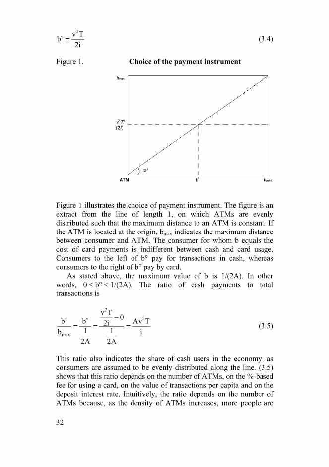
=o (3.4)

Figure 1. Choice of the payment instrument

Figure 1 illustrates the choice of payment instrument. The figure is an extract from the line of length 1, on which ATMs are evenly distributed such that the maximum distance to an ATM is constant. If the ATM is located at the origin, bmax indicates the maximum distance between consumer and ATM. The consumer for whom b equals the cost of card payments is indifferent between cash and card usage. Consumers to the left of b° pay for transactions in cash, whereas consumers to the right of b° pay by card. As stated above, the maximum value of b is 1/(2A). In other words, 0 < b° < 1/(2A). The ratio of cash payments to total transactions is

iTAv

A21

0i2Tv

A21b

bb 2

2

max=

−==

oo

(3.5)

This ratio also indicates the share of cash users in the economy, as consumers are assumed to be evenly distributed along the line. (3.5) shows that this ratio depends on the number of ATMs, on the %-based fee for using a card, on the value of transactions per capita and on the deposit interest rate. Intuitively, the ratio depends on the number of ATMs because, as the density of ATMs increases, more people are

33

located close to ATMs and start to pay in cash instead of by payment card. Similarly, if the card payment fee or the value of transactions per capita increases, paying by card becomes more expensive and more consumers start to pay in cash instead of by payment card. Furthermore, the ratio of cash users depends on the deposit interest rate, which is the opportunity cost of holding cash. Based on (3.5), the ratio of card payments to total transactions is

iTAv1

2

− (3.6)

where 0 < Av2T/i < 1. As the value of total transactions of one consumer is T, and there are N consumers, the total value of card payments is

⎟⎟⎠

⎞⎜⎜⎝

⎛−=

iTAv1NTT

2

card (3.7)

The total stock of average cash holdings in the economy is calculated by multiplying the average cash holdings of consumers that use cash by the share of cash users in all consumers and the total number of consumers, ie by integrating (3.1) divided by two over the cash users, ie from the origin to b° in Figure 1, multiplying this by the density function of b, 2A, and multiplying this by the share of cash users and the total number of consumers, N

3

352

i2Tv

0

2

b

0 max

*2TOT

i3TvNA

Adb2i2

bTi

TAvN

dbb

12

Ci

TAvN2

C

2

=

=

=

∫

∫o

(3.8)

(3.8) indicates that an increase in the number of ATMs will increase the value of cash holdings of consumers.

34

3.1.2 The bank’s decisions

In addition to the consumer’s choice of payment instrument, we need to analyse the profit maximisation problem of the bank. The bank receives revenue from deposits on bank accounts because investing these deposits further in the market yields interest income for the bank. Furthermore, the bank receives revenue from services related to bank accounts, eg fees from card payments. The bank’s costs arise eg from maintaining and developing ATM networks, transporting cash from place to place, and producing payment cards. The bank maximises profits, and banks may compete with each other in terms of price and service level. Examples of competition pricing parameters are the deposit interest rate and the fees charged for card payments. However, in the real world, interest rates seem to have converged to roughly same level. This indicates that banks have competed the pricing parameters to the same level in the industry. Thus banks compete only via service level parameters. In our model, such a relevant service level parameter is the density of the ATM network, ie the number of ATMs, and pricing parameters are assumed to be fixed. In other words, the only relevant decision variable for the bank is the number of its own ATMs. From this profit maximisation point of view, the bank’s aim may well be to reduce the use of cash, promote the use of payment cards, and reduce the number of cash withdrawal ATMs. Consumers’ wealth is assumed to consist of average cash holdings and deposits: TOTTOT D2/CNw += , so that 2/CNwD TOTTOT −= . The bank’s interest rate margin is expressed as )1r( − , where r is the interest rate on the bank’s investment of deposits further in the market, and i is the deposit interest rate paid to the bank’s customers. The income for the bank from card payments is vTcard. Moreover, as stated above, the maintenance of ATMs generates costs to the bank. The costs from serving card payments are excluded because they are mostly fixed costs. At first, the bank must invest in the bank account system, open connections between bank and merchants, etc. After these tasks, the cost of an additional consumer is close to zero. One possibility would be to add a cost per consumer, or a cost per account, to the model, but such costs are presumably very small in the real world, compared to fixed costs. Therefore costs from cards have been excluded from the profit equation. Profits of the bank are modelled using a standard profit function consisting of the income from deposits on bank accounts (interest rate margin times average deposit total), the income from card payments, and the cost of maintaining ATMs

35

AzNTi

TAv1vi3

TvNANw)ir()A(2

3

352

−⎟⎟⎠

⎞⎜⎜⎝

⎛−+⎟⎟

⎠

⎞⎜⎜⎝

⎛−−=π (3.9)

Saving (1977) discusses the bank’s profit maximisation problem, and this part of our model is quite similar to Saving’s model. Saving (1977) assumes that the bank receives income from deposits and that the provision of banking services also generates some costs to the bank. In addition to these factors, we include income from payment cards in (3.9). Equation (3.9) shows that it is optimal to reduce the number of ATMs to zero10. We assumed that consumers require both cash and card payment alternatives. In order to make cash transactions, consumers need ATMs because they are assumed to be the only cash distribution channel in the economy. If the bank decides to reduce the number of ATMs to zero, consumers do not keep any funds in their bank accounts. Thus no bank reduces ATMs to zero alone if there are other banks and other ATM networks in the market. This indicates that if there is monopolisation in the industry, the number of ATM decreases. One approach for including competition in (3.9) is to assume that the bank’s market share depends on the number of its ATMs. Denote the number of bank k’s ATMs as Ak and the number of other banks’ ATMs as BA

kjj =∑

≠. The market share is assumed to equal the

number of the bank’s ATMs (Ak) divided by the total number of ATMs in the industry )BA( k + . As in the monopoly case above, ATMs are assumed to be evenly distributed along the line of length 1 such that the maximum distance to the nearest ATM is constant,

))BA(2/(1 k + . The consumer is assumed to first notice the closest ATM and the distance to it, then to select the bank, and finally to decide on the payment instrument. Therefore both deposits and card payments of one bank will depend on its market share. In the competitive case, the profits of bank k are expressed as

10 The number of ATMs, A, appears only in the numerator and is always subtracted. So, if the number of ATMs increases, the profits of the bank decrease. Furthermore, both the first and second derivatives with respect to the number of ATMs are negative. Thus profits are maximised when the number of ATMs is zero.

36

zANTi

Tv)BA(1v))BA/(A(

i3Tv)BA(NNw)ir))(BA/(A()B,A(

k

2k

kk

3

352k

kkk

−⎟⎟⎠

⎞⎜⎜⎝

⎛ +−+

+⎟⎟⎠

⎞⎜⎜⎝

⎛ +−−+=π

(3.10)

Differentiating (3.10) with respect to Ak yields the optimal number of ATMs of bank k.11 The resulting function is, however, highly complicated and difficult to interpret. Contrary to (3.9), (3.10) does not indicate a corner solution. Appendix 1 discusses the first and the second derivatives of (3.10) as indicating that the profits of bank k are maximised. Figure 2 shows an example of the graph of (3.10)12. Figure 2. Maximum profits and the optimal number of ATMs in the competitive case

-15000

-10000

-5000

0

5000

10000

15000

20000

0 40 80 120

ATMs

Prof

its

Our primary interest is to examine how the change in the number of other banks’ ATMs, B, affects the optimal number of one bank’s ATMs, Ak. The implicit function rule says that even if the specific form of the implicit function is not known, its derivatives can be found by taking the negative of the ratio of a pair of partial derivatives of the function which defines the implicit function (eg Chiang 1984, p. 208). In this case, we assume that the implicit function is the first 11 The optimal number of ATMs can be seen as a Nash equilibrium (eg Varian 2002, p. 499–500). In other words, each banking group decides the number of its own ATMs given the choice of other banking groups. None of the banking groups knows what other banking groups are going to do when they have to decide the number of their own ATMs. However, when the choices of other banking groups have been revealed, none of the banking groups is willing to change its choice. 12 B = 100; r = 0.03; i = 0.01; w = 10000; v = 0.001; T = 10; z = 1000, N = 1000.

37

derivative of the profit maximisation function (3.10) with respect to Ak and that it is equal to zero. The implicit function rule can be applied as

k

k2

2k

A

B

y

x A

A

BAFF

FF

k

Δ=

⎟⎟⎟⎟⎟

⎠

⎞

⎜⎜⎜⎜⎜

⎝

⎛

∂π∂∂∂

π∂

−=−=− (3.11)

This equation indicates how the optimal number of one bank’s ATMs, Ak, changes as the number of other banks’ ATMs, B, changes. In order to include the number of ATM networks in this model we assume that there are m banks, or banking groups, in the industry and that each bank has its own ATM network. In the symmetric case, all banks are similar to each other and the number of ATMs is the same for each. In this case, the number of other banks’ ATMs can be expressed as A)1m(B −= . If a new bank enters the market, the number of its ATMs affects the number of ATMs of all other banks. Each bank will either decrease or increase the number of its own ATMs and, moreover, the number of the ATMs of the entering bank increases the total number of ATMs in the industry. The change in the number of one bank’s ATMs, ∆A, can be expressed as

))rwTv)(m1(i6

w)m1(i6vTrmA2vTimA2(

/))rwTv)(m2(i3

w)m2(i3vTrmAvTimA(A

3

453325332

3

453325332

++−−

+−+−

++−+

+−−+−=Δ

(3.12)

Equation (3.12) indicates that the change in the number of ATMs of one bank is negative as a new bank enters the industry (A, m, T, v, w, i and r are positive, m > 1, and r exceeds i). However, based on our research question, we are interested in how the number of ATMs in the whole industry changes if a new bank enters the industry. This effect can be analysed by multiplying the change in the number of one bank’s ATMs by the number of ATM networks and adding the entering bank’s ATMs in the equation

38

))rwTv)(m1(i6w)m1(i6

vTrmA2vTimA2(

/))w)ir(Tv)(m2(mi3

)w)ri(Tv)(m1(Ai6

vT)ri(mAvT)ri(mA2(AAm

34

53325332

3

3

53425333

++−−+−+

−

−++−+

−+−+−+

+−+−=+Δ

(3.13)

Because the number of ATMs, A, exceeds the number of ATM networks, m, and r > i, both the numerator and the denominator are negative, and so the RHS of equation (3.13) is positive. In other words, if a new bank enters the market, the total number of ATMs in the industry increases. Similarly, monopolisation decreases the total number of ATMs in the industry. One way to analyse the effects of other parameters in the model would be to differentiate the optimal number of ATMs with respect to the number of consumers, the value of transactions per capita and the payment card fee. However, these differentiations yield highly complicated results that do not enable us to analyse whether the effect on the optimal number of ATMs is positive or negative. However, based on our research question, the most important result of the above analysis is that a decrease in the number of ATM networks reduces the number of ATMs. The other finding is that card payments replace cash payments. If customers increase the use of cards, ceteris paribus, the use of cash decreases. In this case, a rational bank reduces the number of its ATMs because it receives more income from card payments and ATM maintenance costs reduce the bank’s profits. Thus the relationship between card payments and ATMs is assumed to be negative. Furthermore, the effect of ATMs on the cash usage is found to be positive based on equation (3.8). Intuitively, we could also assume that cash in circulation affects the number of ATMs. The dependence between ATMs and cash might be presumed positive because the more that people use cash, the more they would probably need ATM services. However, the effect of cash on the number of ATMs is not so straightforward. For instance, in Finland, cash in circulation has been steadily increasing, except for just before the euro changeover, even though the number of ATMs has been declining since the 1990s. This indicates that the dependence between cash and ATMs is not necessarily positive. Part of cash in circulation may be in passive use, ie not used for transactions. Thus, we assume the number of ATMs and cash in circulation to relate to each other positively or negatively.

39

The discussion above indicates that in the competitive case banks maintain ATM networks, and the number of ATMs is greater than zero. For simplicity, we analyse the case of two banks, or banking groups, and the competition between them. As in many other competitive cases, this problem seems to be a prisoner’s dilemma (Figure 3). Figure 3. Prisoner’s dilemma: competition between two banks

Number of ATMs of Bank 2 0 1

Number of ATMs of Bank 1

0 (100, 100) (0, 150)

1 (150, 0) (50, 50)

We assume that customers select a bank on the basis of availability of services, ie the density of the ATM network. If both banks decide to provide no ATMs to customers, the payoff of both banks is 100 in Figure 3. However, if one of the banks installs one ATM, it gets all the customers in the market. In other words, this bank receives the income of both banks (200) and has to pay the cost of establishing an ATM network (50). In other words, if one of the banks installs an ATM and the other one does not, payoffs of the banks are 150 and 0, respectively. However, this is not an equilibrium. The other bank also decides to install an ATM, in order to get the original customers back. Therefore, in equilibrium both banks provide ATM services with payoffs (50, 50), even if the payoffs would be higher with no ATMs (100, 100). This simple example clearly indicates that in the competitive case the number of ATMs in equilibrium exceeds zero. In other words, monopolisation reduces the optimal number of ATMs, which was indicated also by (3.13) above.

40

3.2 Transaction-size model

In this section, we present an alternative model of the consumer’s choice of payment instrument. To do this, we introduce the idea of Whitesell (1989), in which small transactions are assumed to be paid in cash and large transactions via alternative payment methods. Cash is considered to be a suitable payment instrument for small-value payments because there are some fixed costs associated with the alternative payment methods. Furthermore, eg the risk of theft discourages large cash holdings. Because the size of the transaction determines the payment instrument, we call this alternative model the transaction-size model. In this model, consumers are assumed to be identical. 3.2.1 The consumer’s decisions

Whitesell (1989) assumes that there are two assets: currency and an interest-bearing account that is drawn on by check, debit card or credit card. It is assumed that transactions vary in size and that the consumer pays for transactions of various sizes with various payment instruments. Transactions of each size occur at a uniform rate over a unit period. Currency will be used for the smallest transactions, and Whitesell (1989) denotes the largest payment made by currency by λ. The consumer decides the optimal λ and the number of cash withdrawals. Total spending during the period is

∫∞

=0

dT)T(FY (3.14)

where F(T) is the value of spending on transactions of size T during the period. We assume that the integral is convergent. The value of spending in cash during the period is expressed as

∫λ

=0

dT)T(FS (3.15)

Transactions larger than λ are paid with other payment instruments. Whitesell (1989) introduces a complex cost structure for alternative payment instruments, assuming that costs consist of fixed and variable

41

costs. According to Whitesell, the total cost of transacting a purchase of size T is u + vT. The consumer minimises the total cost of cash and card payments

dT)Tuv)(T(FdT)T(F

n2inbmin

0∫ ∫λ ∞

λ

+++ (3.16)

where n is the number of cash withdrawals, b the fee of withdrawing cash, i the interest rate for deposits, F(T) the value of spending on all transactions of size T during the period, and v + u/T the cost of transacting a purchase of size T by payment card. In order to introduce ATMs into the model, we express cost b as a function of the number of ATMs: b = 1/A. The first order conditions of the cost minimisation problem with respect to λ and n are

0)uv)((Fn2

)(iF =λ

+λ−λ (3.17a)

0n2iS

A1

2 =− (3.17b)

Based on these first order conditions, the average value of cash holdings is

A)uv(2

1iA1n

n2S

2C

λ+

===∗

(3.18)

This equation indicates that an increase in the number of ATMs reduces the value of consumers’ cash holdings. This is the opposite result from that of the spatial model (3.8). This opposition of results could stem from the different natures of the two models. In the spatial model, if the number of ATMs increases, there are more people located close to ATMs. Thus part of the population starts to pay in cash instead of using payment cards, and the average cash holdings increase based on (3.8). In the transaction-size model, if the number of ATMs increases, the consumer increases the number of ATM withdrawals because it is more convenient to visit the ATM. Thus the average value of cash holdings decreases, as indicated by (3.18).

42

In order to formulate an explicit function for cash demand and profits, and to analyse the bank’s optimisation problem, we should make some assumptions about the transactions distribution. One could assume that the value of transactions is the same in each category. But Whitesell (1989) discusses a special case where the number of transactions is the same in each size category. However, such assumptions about the transactions distribution restrict the results and, furthermore, the analysis becomes more complicated. Therefore, we have not introduced any special transactions distribution in this model. Even if we do not analyse a bank’s profit maximisation function formally, some implications are evident. In this case, the profit function also in the monopoly would depend both positively and negatively on the number of ATMs. This indicates that the optimal number of ATMs would not be zero even for a monopoly bank. However, the optimal number of ATMs must be a finite number, as there are maintenance costs depending on the number of ATMs in the profit function. 3.3 Comparison between spatial and

transaction-size models

The spatial model and the transaction-size model discussed in Sections 3.1 and 3.2 differ to some extent and produce somewhat contradictory results. According to the spatial model, an increase in the number of ATMs increases cash holdings (3.8), whereas the transaction-size model gives the opposite result (3.18). Moreover, the earlier literature includes contradictory empirical results on the influence of ATMs on cash demand, as summarised in Section 2.2.3. On the one hand, ATMs may reduce cash in circulation because it is convenient to withdraw cash so that people keep less money in their wallets. On the other hand, because it is convenient to withdraw money, people may use cash instead of other payment instruments, which may increase cash in circulation. Moreover, ATMs are part of the retail payment system, and the development of other retail payments affects cash usage and the need for cash withdrawal ATMs. Profits of the monopoly bank in the spatial model (3.9) seem to lead to the corner solution, suggesting that it is optimal for the bank to reduce the number of ATMs to zero. However, if we introduce market share as a function of the number of ATMs in the spatial model, there is an interior solution (3.10). (3.13) indicates that monopolisation leads to a smaller number of ATMs. In other words, the optimal

43

number of ATMs in monopoly is lower than the optimal number of ATMs in the competitive case. This is in line with the industrial organisation theory discussed in Section 2.3. However, we have assumed that the number of ATMs is the bank’s only decision variable. If we included other decision variables, such as the level of the deposit interest rate, the number of employers or the number of bank branches, the results might change. However, because the most interesting and the most essential decision variable here is the number of ATMs, other decision variables are not included in the model. Do ATM networks and the number of ATMs then have any role in the competition between banks? It seems that they do because banks maintain large networks. Even in the monopoly case – even if it seems to be optimal to reduce the number of ATMs to zero in some cases – banks hold more than zero ATMs. This may be rational because, if banks do collude, some banks would have incentives to leave the collusion and establish their own networks, if the services provided to customers were insufficient. So, if the collusion really maximises the profits of its members, the optimal number of ATMs is not zero. Furthermore, as the market share of the bank depends on the services it provides to customers, the number of bank branches and ATMs may influence this market share. In the competitive case, the bank with the most ATMs might win the competition and get all the customers. This would lead again to the monopoly case where the bank has incentives to reduce the number of ATMs to zero. However, this is not an option, due to the threat of entry. In other words, there must be some equilibrium number of ATMs in the market because otherwise a rival will enter the market and take all the customers. A low level of electronification may neutralise the effects of monopolisation in the ATM network market. Electronification of retail payments can be described as follows. In the first phase people receive salaries and other income in cash and pay for everything with cash. When the number of bank accounts increases, salaries are paid directly into bank accounts. People use cheques or other paper-based retail payment instruments and withdraw cash at ATMs. In this phase, monopolisation of the ATM industry does not necessarily decrease the number of ATMs. This may occur because banks probably have incentives to keep people using ATMs instead of reversing back to the bank branches to withdraw cash. In the next phase, people start to use payment cards instead of cash, and banks have incentives to promote electronification of payments eg by reducing the number of ATMs. Furthermore, people pay their invoices by electronic credit transfers or direct debits, which further reduce the demand for cash. In the end, all transactions are handled electronically and cash vanishes. However,

44

cash has some special features, like anonymity, and therefore it is unlikely to vanish totally. Typically, countries are in different phases of electronification development. For instance, the Nordic countries have highly developed retail payment systems and electronification is generally at a high level compared eg to other European countries. There are some aspects that could be included in the models discussed in Sections 3.1 and 3.2. For instance, in the spatial model, the consumer’s payment instrument choice depends on the location of the nearest ATM related to the consumer. If we assume that the consumer does not move, the initial location completely determines the selection of payment instrument. This problem could be eliminated by assuming consumers to move along the line in a way that they are still evenly distributed13. Then, the representative consumer would, with positive probability, be at his initial spatial location and would truly have a possibility of selecting either cash or card every day, depending on his new location. This may have no effect on the final results, but it is one way to revise the assumptions of the model. Furthermore, some strict assumptions are made in connection with the transaction-size model. First, the limit λ may be difficult to discover in reality. For technical and legal reasons, there is no explicit upper limit on cash payments. Also empirical studies such as Virén (1993), indicate that no such limit can be found. However, there have been some lower-value limits on card transactions. For instance, in Finland, the value of a card transaction previously had to exceed ca EUR 5. Nowadays, there are neither cash nor card payment limits, and the average size of a debit card payment has decreased during last few years (Finnish Bankers’ Association 2004). Furthermore, the cost structure of alternative payment instruments is very complicated in the original model (Whitesell 1989). Including a simpler cost structure, for example only %-based cost for card payments, would possibly have some influence on the final results.

13 For instance, in the spatial models by Massoud and Bernhardt (2002) and Croft and Spencer (2003) the consumer is assumed to move such that with some probability he is at his initial spatial location.

45

3.4 Implications for empirical work

The theoretical discussion based on the spatial and transaction-size models provides some implications for empirical work. First, the number of ATM networks affects positively the number of ATMs, as indicated by (3.13). In other words, the monopolisation of ATM network market structure leads to a smaller number of ATMs. Also the earlier studies of various industries indicate that monopolisation leads to higher price and lower service levels, as discussed in Section 2.3. However, the corner solution suggested by the spatial model in the monopoly case (3.9) is an extreme result, which is not observed in reality. The profit function does not necessarily include all relevant, consumer relationship -related factors. If banks decided to reduce the number of ATMs to one or even zero, legislators or competitors would obviously inhibit these plans. In addition to ATM networks, the number of ATMs apparently depends on certain scale variables, such as the size of the country. The larger the country, the greater the cost of transporting cash from one place to another. We could assume that the number of ATMs depends negatively on maintenance expenses. However, the costs of maintaining ATMs or data on the prices of alternative payment instruments are not available for estimations, as discussed in Section 2.5. We also assume that if the usage of payment cards increases, the optimal number of ATMs decreases, as there is less demand for cash and cash withdrawal ATMs. Furthermore, cash in circulation may affect the number of ATMs. In order to minimise the number of independent variables, we concentrate on the most relevant ones based on our research question

)card,cash,m(fA/ −−++

= (3.19)

Based on our theoretical results, cash in circulation depends, either negatively or positively, on the number of ATMs. This ambiguous result is not a surprise: cash usage has been discussed in the earlier empirical literature and, based on this discussion, the effects of ATMs on cash in circulation are contradictory. Some results indicate that the use of cash decreases when there are more ATMs, whereas some results indicate the opposite. Empirical work with our data set may provide more evidence on the question of whether the influence of ATMs on cash in circulation is positive or negative. In addition to ATMs, cash depends, based on (3.8), positively on the value of transactions per capita and negatively on the deposit interest rate.

46

GDP per capita will be used as a proxy for the value of payment transactions per capita. Furthermore, cash in circulation tends to depend negatively on the value of card payments, which are a substitute for cash payments. Based on (3.8) and (3.18), we include the following parameters in the cash equation

)card,i,T,A(fcash/ −−+−+

= (3.20)

47

4 Empirical evidence In this section, we make both pooled and panel data estimations with annual data on 20 countries14. For most countries, the data are available for 1988–2003 or 1990–2002. Based on the discussion in earlier sections, we make the following hypothesis: 1) The reduction of ATM networks, ie the monopolisation of ATM network market structure, reduces the number of ATMs. 2) Cash demand depends, either negatively or positively, on monopolisation of the ATM network market structure. This needs to be tested with the data because the impact of ATMs on the value of cash holdings is somewhat ambiguous. Overall, it is worth testing whether the results indicated by the theoretical discussion are supported by the actual data. 4.1 Data description

The data set to be used includes eg numbers of ATMs and ATM networks, cash in circulation, value of debit and credit card transactions, deposit interest rate, population, and GDP in real and nominal prices. Main data sources are the statistics published by the ECB15, BIS16, Finnish Bankers’ Association17, central bank of Norway, and Eurostat. The number of ATM networks differs across countries. In some countries, there is only one network, whereas in some countries there are dozens of them. Overall, the number of ATM networks is very low in the European countries, with the exception of Greece. For example, in the UK the number of ATM networks fell to one at the end of the 1990s and in Spain there are three networks. In contrast, the number of ATM networks is high in Canada and in the USA – tens of ATM networks in both. The development of ATM networks has differed to some extent between countries. Moreover, the ATM network seems to 14 Austria, Belgium, Canada, Denmark, Finland, France, Germany, Greece, Ireland, Italy, Japan, Luxembourg, Netherlands, Norway, Portugal, Spain, Sweden, Switzerland, UK, USA. 15 ECB 2004, ECB 2002, ECB 2000, EMI 1996. 16 BIS 2004, BIS 2002, BIS 2001, BIS 1997, BIS 1996, BIS 1995a, BIS 1995b, BIS 1994, BIS 1993. 17 Finnish Bankers’ Association 2004, Suomen Pankkiyhdistys (SPY) 2001, SPY 1992, SPY 1990, SPY 1989.

48

be somewhat difficult to define. There may be one ATM network maintained by one company, which is jointly owned by the banks. On the other hand, there may be two brands in common use, ie customers of both brands can withdraw cash at all ATMs independent of its brand, and this is free for customers. Some countries define such a structure as a single ATM network. Furthermore, some countries also consider as networks those that are provided as special services solely for the bank’s own customers and not for common use, whereas some countries do not include such networks in the statistics.18 It would be interesting to analyse only the nationwide networks. However, the problem with ATM networks is that the number of open and limited access ATMs has not been separated for all countries over 1988–1995. Therefore, we need to use the total number of ATMs for the whole period. Also the numbers of nationwide and regional ATM networks have not been reported for all countries and all years. Therefore, we decided to use the total number of ATMs and ATM networks in our estimations. We briefly describe the development of ATM network market structure in each country in Appendix 2. The first cash withdrawal ATMs were installed already in the 1960s eg in the USA, UK, Canada, Japan and Sweden. Typically, the first ATM networks were not compatible and banks provided services only to their own customers. Subsequently, the compatibility of ATM networks has increased, and there are nationwide ATM networks that provide services to all banks’ consumers. The number of ATMs has been increasing in most of the countries discussed in this study. Finland is the only country where the number of ATMs has considerably decreased during the observation period. The number of ATMs decreased during 1993–2003 from ca 3000 to ca 2000. In fact, Finland is the only country where the number of ATMs was higher in 1990 than in 2002. In many countries, the number of ATMs has 18 In our estimations, we used the data on ATM networks that are available in ECB and BIS statistics. However, there are some exceptions. The number of ATM networks is one in Germany because it has been changed from four to one backwards in the statistics for year 2004. According to the central bank of Germany, this was done because the interpretation of ATM network has changed. So there have not been any changes in the actual number of ATM networks. Italy seems to be a similar case because they have changed the number of ATM networks backwards from one to four (four networks since 1996 or 1999, depending on the data source). We used four networks for Italy since 1996, and before that n.a. For Japan, we used data for the period 1988–1999 because there have been changes in the method of data collection, and the data since 2000 are not consistent with the data up to 1999. For Finland, the number of ATM networks reported in the statistics has been one since 1994. However, there have been two other, small networks that were closed down in 2004. Because networks have been interoperable, we have not changed this series.

49

increased notably during 1990–2002. For example, the number of ATMs in the UK increased during this period from ca 17000 to ca 41000, in Portugal from ca 800 to ca 11000, and in Belgium from ca 900 to ca 7000. In Sweden and Norway, the number of ATMs has been increasing moderately, and in Norway the number of ATMs in 2003 was less than in 2002. In order to compare numbers of ATMs in various countries, we scaled the numbers by million inhabitants. This figure for 2002 is lowest for Sweden (ca 300) and highest for Spain, Canada and the USA (over 1200 ATMs per million inhabitants). The number of ATMs per million inhabitants in Finland has decreased from ca 600 in 1993 to ca 400 in 2002. However, the number of ATMs per million inhabitants alone cannot be considered to indicate the availability of ATM services. The ratio may be high because of many incompatible ATMs. Furthermore, ATM services may be well available if all ATMs are compatible, even if the number of ATMs per million inhabitants is low. The number of ATM withdrawals and the average value of an ATM withdrawal indicate the usage of ATMs. The number of ATM withdrawals per capita increased in most of the countries during the observation period. However, the increase in the number of ATM withdrawals has stabilised in some countries, and has started to decrease eg in Finland and Canada in the 2000s. In 1990, the number of ATM withdrawals per capita was lowest in Italy and Japan (less than 2), and highest in Canada, Sweden, USA and Finland (20–23). In 2002, the ratio was lowest for Japan (ca 3 transactions per capita), Italy (11), Luxembourg and Austria (13). During the observation period, the average value of an ATM withdrawal was lowest in Canada (ca EUR 40–60) and in the USA (ca EUR 50). The average value of a cash withdrawal was also low in Finland and France. Of the European countries, the average withdrawal in 2002 was highest in Italy, Greece, Germany and Switzerland (ca EUR 160). Contrary to the number of ATM withdrawals, the average value of an ATM withdrawal has been quite stable in most countries. In other words, the growth in the number of ATM withdrawals has been about as rapid as the growth in the value of withdrawals in most countries. Banks may have incentives to decrease the number of ATMs if customers often withdraw small amounts of cash and there are no withdrawal-based charges. Cash in circulation is also a relevant variable in our study. To be able to compare cash in circulation in various countries, we need to scale it. Suitable scaling factors would be GDP or population, with cash converted into a single currency. Cash in circulation per GDP or

50

private consumption has remained fairly stable in most countries in 1988–2001. However, cash in circulation decreased in euro countries in 2000–2001 because of the euro conversion. Since 2002, cash in circulation in individual euro countries has not been available, as only the total value of euros issued is published in the statistics. Cash in circulation per capita also decreased considerably in euro countries before the euro conversion. During the 1990s, the value of cash per capita was lowest in Portugal and Finland, increasing from ca EUR 300 per capita to ca EUR 500 per capita. In many countries, this ratio totalled ca EUR 1000 at the beginning of the 2000s. Cash in circulation per capita has been highest in Japan (ca EUR 4000 per capita in 2003) and Switzerland (ca EUR 3200 per capita in 2003). Cash in circulation per GDP has been lowest in Finland (ca 2% in 1988–2001). This ratio has been highest in Japan (ca 14.5% in 2003), Switzerland (ca 8% in 2003), and Spain (ca 10% in 1994–1999). Numbers and values of card payments are also relevant variables because card payments are used as substitutes for cash payments. The number of debit and credit card payments per capita was high in the USA, Canada and Finland in 1988–2003. Card payments are popular also in Norway, Denmark and UK. The number of card payments per capita is lowest in Greece, Italy, Japan and Austria. The growth of card payments was very rapid in most countries during the observation period. Also based on the value of card payments per GDP, card usage is most popular in the USA, Canada, UK, Portugal, Norway, Sweden and Finland. Again, card usage is at the lowest level in Greece, Japan and Austria. Relative importance of ATM withdrawals can be seen by dividing the number of ATM withdrawals by the number of card payments. This ratio was less than one eg in the USA, Canada and Finland in 1988–2003. In other words, card payments have been important in these countries during the whole observation period. The relative importance of ATM withdrawals compared to card payments has been decreasing considerably in the Netherlands, Spain, Sweden, Italy, Austria and Germany. One way to illustrate the level of electronification is to compare the number of ATMs to the number of card payments (Figure 4). ATMs are considered to indicate the usage of cash, and cash or cheque usage can be replaced by card payments. According to this comparison, Finland, Norway and Denmark are at the highest level of electronification. In these countries, there are lots of card payments and relatively few ATMs per capita. In the USA and Canada, the number of card payments is high but, at the same time, there are many ATMs compared to other countries. Card usage is at a low level in Greece, Italy, Spain, Germany, Austria and Japan.

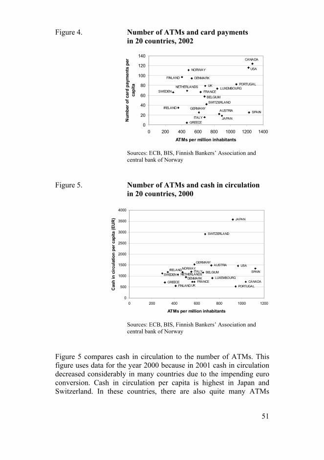
51

Figure 4. Number of ATMs and card payments in 20 countries, 2002

DENMARK

SPAIN

FRANCE

NORWAY

PORTUGAL UK

AUSTRIA

BELGIUM

CANADA

GERMANY

FINLAND

GREECE

IRELAND

ITALY JAPAN

LUXEMBOURGNETHERLANDSSWEDEN

SWITZERLAND

USA

0

20

40

60

80

100

120

140

0 200 400 600 800 1000 1200 1400

ATMs per million inhabitants

Num

ber o

f car

d pa

ymen

ts p

er

capi

ta

Sources: ECB, BIS, Finnish Bankers’ Association and central bank of Norway Figure 5. Number of ATMs and cash in circulation in 20 countries, 2000

AUSTRIA

BELGIUM

CANADAFINLAND

GREECE

ITALY

JAPAN

LUXEMBOURGNETHERLANDS

PORTUGAL

SWITZERLAND

USAGERMANY

DENMARK

SPAIN

FRANCE

IRELANDNORWAY

SWEDEN

UK

0

500

1000

1500

2000

2500

3000

3500

4000

0 200 400 600 800 1000 1200

ATMs per million inhabitants

Cas

h in

circ

ulat

ion

per c

apita

(EU

R)

Sources: ECB, BIS, Finnish Bankers’ Association and central bank of Norway Figure 5 compares cash in circulation to the number of ATMs. This figure uses data for the year 2000 because in 2001 cash in circulation decreased considerably in many countries due to the impending euro conversion. Cash in circulation per capita is highest in Japan and Switzerland. In these countries, there are also quite many ATMs

52

compared to the population. Both cash in circulation per capita and the number of ATMs per million inhabitants are low in Finland. In addition to payment systems data, the data on deposit interest rates in each country are relevant because deposit rates affect cash in circulation based on (3.8). The deposit interest rate declined in many countries during the 1990s. In most countries, the rate has been under 10% during the whole observation period. The deposit interest rate was highest in Greece and Portugal (even 20% in Greece at the beginning of the 1990s) but has declined there in recent years, to 2%–3%. 4.1.1 Availability of data

The availability of data differs to some extent across the countries. The data on ATMs per population are available for years 1988–2003 for Belgium, Canada, Germany, Finland, France, Italy, Japan, Netherlands, Norway, Sweden, Switzerland and UK. These data are available for 1990–2002 for Austria, Spain, Greece, Ireland, Luxembourg and Portugal. For the USA, the data are available for 1988–2002, and for Denmark 1991–2002. The data on ATM networks in some countries are missing for some years (eg for Austria and Portugal these data are available for 1990–1995 and for France 1988–1995). Data on payment card transactions are not available for Greece for 1990–1992, 1994 and 1999; for Ireland 1997; for Japan 1988 and 2003; for Luxembourg 1990, 1992–1993 and 1995; and for the UK 1988. Other data on card transactions are available as for the number of ATMs. Cash in circulation is available for euro countries up to 2001 and for other countries for the whole period. Data on deposit interest rate are missing for some countries for the last years of the observation period (eg for Austria and Portugal after 2000). Population, as well as GDP in real and nominal prices, are available for the whole observation period for all countries. Because of data shortages and variable transformations, the number of observations used in the estimations is about 200. Furthermore, there seem to be some changes in series that cannot be chained. Figures on the data series are presented in Appendix 3.

53

4.2 Equations to be estimated

In this section, we present the ATM and cash equations to be estimated. These two equations indicate how changes in ATM network market structure affect the availability of ATM services and cash in circulation. Our aim is to keep the equations as parsimonious as possible. Before presenting the ATM and cash equations, we discuss the dynamic specifications of the model. 4.2.1 Dynamic model specifications

One approach to analyse the dynamic structure of the model is to use the traditional and popular partial adjustment model (eg Davidson and MacKinnon 2004, p. 576–577). The idea of the partial adjustment model is that there is some desired level for the dependent variable, and the dependent variable adjusts towards this desired level. The desired level of yt is yt˚, which depends on a vector of exogenous variables Xt

ttt eXy +β= oo (4.1) The adjustment towards the desired level is given by

t1tt1tt v)yy)(1(yy +−δ−=− −−o (4.2)

where the adjustment parameter δ needs to be positive and less than 1. Solving these two equations yields

t1tt

ttt1t1tt

uyXve)1(X)1(y)1(yy

+δ+β=+δ−+βδ−+δ−−=

−

−−o

(4.3)

where oβδ−≡β )1( and ttt ve)1(u +δ−≡ . As seen, in (4.3) the one-period lagged dependent variable is in the right-hand side of the equation. The coefficient of each variable in logarithms indicates the short-run elasticity. The long-run elasticity can be calculated by dividing the coefficient by one minus the adjustment parameter, ie one minus the coefficient of the one-period lagged dependent variable (eg Greene 2000, p. 722). This partial adjustment model might provide a suitable dynamic structure for our equations. The number of ATMs in

54

the previous period does certainly affect the number of ATMs in the current period, and the same holds for cash in circulation. Furthermore, we are interested in both short and long-run elasticities. Our theoretical discussion in Section 3 did not suggest any specific lag structure for the estimations. One approach is to estimate the ATM and cash equations without any lags but, based on our estimations, the fit of equations is much better if one period lagged dependent variables are included as explanatory variables. Furthermore, more than one-period lagged values of the dependent variable or lagged values of independent variables may be usefully included in estimations. For instance, in the ATM equation the reduction of ATM networks may affect the number of ATMs in the following period. We estimated equations with more lags but the one-period lagged dependent variable as an independent variable seemed to work well. Moreover, our data is annual, the observation period is quite short, and there are many variables to be estimated. In order to keep the model as parsimonious as possible, it is better not to include too many lagged variables in the equations to be estimated. Thus we introduce one-period lagged dependent variables as explanatory variables in both the ATM equation and the cash equation and hence employ the partial adjustment model. When using panel data, one must decide whether to include fixed effects in the estimations. There may be country-specific factors that influence the payment system developments. However, there is no theory indicating which country-specific factors should be included. One approach is to use dummy variables that reflect the effects of omitted variables specific to individual countries but remain constant over time (eg Hsiao 2003, p. 30). However, the use of fixed effects is not problem-free because fixed effects invalidate the cross-section analysis of countries. On the other hand, because not all relevant country-specific factors can be identified, it would be reasonable to include fixed effects in level estimations. When estimating the equations in first differences, the constant-over-time fixed effects disappear. Therefore, estimations in first differences may be preferable because not all fixed effects can be modelled. Country-specific, omitted factors that affect the dependent variable may also be included in the model as random effects. In other words, these factors are not included as independent variables in the model but are summarised by a random disturbance (Hsiao, 2003, p. 34). Furthermore, it is not self-evident whether we should include fixed or random effects in our estimations. Hsiao (2003, p. 41) states that, if the observation period is very long, the fixed and random effects lead to the same estimate. However, our observation period is quite short.

55

We estimated our equations with both fixed and random effects, and the results of both were quite similar. The level estimation results with and without fixed effects are presented in Section 4.3. In addition to the lag structure of the model, we need to decide whether to estimate the equations in levels or differences. The differencing test (eg Krämer and Sonnberger 1986, p. 101–103) compares level estimates to first difference estimates and indicates whether the model results the same coefficients in both cases. The basic idea is that the second differences of explanatory variables are added in the level estimation. We performed the differencing test and used the Wald coefficient test to study whether the coefficients of second differences differ from zero. Based on the test results, the null hypothesis that the coefficients of second differences are zero cannot be rejected. This test result legitimates reporting both the level and difference estimation results for both the ATM and cash equations. However, Krämer and Sonnberger (1986) point out that a constant term and lagged dependent variable may lead to problems with the differencing test. We also performed the unit root tests on all variables. Based on the pooled unit root tests, all variables used in the ATM and cash equations are stationary in first differences but not necessarily in levels (Appendix 4). We estimate the ATM and cash equations in both levels and first differences in Section 4.3 to see whether the coefficients are similar in size and sign. 4.2.2 ATM equation

The number of ATMs depends on banks’ decisions about size of the ATM network. Banks need to decide how extensive an ATM network they are willing to maintain. This decision is, at least to some extent, a response to customers’ demand for ATMs. The number of ATMs is presumed to depend on competition between banks or ATM networks, on consumer’s demand for various payment instruments, and on demographic variables. Our theoretical discussion provided some implications for empirical work on the ATM equation, as summarised in Section 3.4. Industrial organisation theory indicates that monopolisation of an industry leads to lower quantity and higher price of product. In this case, the product is the availability of ATM services, ie the number of ATMs. Also, our spatial model indicates that the optimal number of ATMs is less in the monopoly case than in the competitive case. Based on this, we assume that a decrease in the number of ATM

56

networks – ie a decrease in the level of competition19 – leads to a decrease in the number of ATMs. If the number of ATMs decreases, there is at least an inconvenience cost to consumers. On average, the distance between consumer and ATM increases. Monopolisation may also entail financial costs to consumers because it may be easier to start pricing for services if there is no competition in the ATM network market. The values of debit and credit card transactions are included in the ATM equation because payment cards are a substitute for cash. The more people use payment cards, the less the demand for cash and ATMs. Also cash in circulation may have effect on the usage of ATMs and the number of ATMs. If cash in circulation increases, people may make more cash withdrawals at ATMs20. The most relevant demographic indicator would be population density. In some countries, most of the population is concentrated in certain cities, whereas some regions are very sparsely populated. One population density indicator is the figure indicating the portion of population living in cities. However, the share of people living in cities was very stable during the observation period. The share of population living in cities is an example of a country-specific variable in the level estimations that is almost independent of time. Therefore, this factor may be included in fixed effects in the estimations, rather than as a separate parameter to be estimated. Because the ATM equation is the major novelty of this study, we estimate two versions of this equation. Based on the discussion above, the number of ATMs should depend on the number of ATM networks and on the one-period lagged number of ATMs. In addition to these variables, the number of ATMs may depend on cash in circulation and payment card transactions. Because we use data on 20 countries, we use relative figures. If we introduce population as a scaling factor, cash in circulation and the value of card payments need to be converted into the same currency, in this case into euros. Currency in circulation declined considerably in euro countries before the euro conversion. Therefore, we introduce a euro dummy in the equations that include the variable cash in circulation. This dummy is zero for 19 Some concentration indicator, like Herfindahl index or CR5 of the banking sector, could also be used as a competition indicator. However, no concentration indicator has been used because of the lack of data. Furthermore, the number of bank branches could be an interesting variable because it depicts the ease of withdrawing money at a teller. However, a lack of data also hinders the inclusion of bank branches in the estimations. 20 However, some cash is in passive use, eg hoarded (= cash holdings used as a store of value) in the home country or in the currency area, or hoarded abroad or outside the currency area. Furthermore, some cash may be used in illegal transactions.

57

1988–2000 and one from 2001 for euro countries, and zero for the whole period 1988–2003 for countries that did not adopt the euro. Two versions of the ATM equation are estimated in log-linear form

jt1jtjtjjt alnmlnaln ε+γ+β+α= − (4.4a)

jtjt1jtjtjtjtjjt dalnzlnxlnmlnaln ε+μ+γ+ρ+θ+β+α= − (4.4b) Based on the discussion in Section 4.2.1, we estimate these two versions of the ATM equation also in first differences

jt1jtjtjt alnmlnaln χ+Δγ+Δβ=Δ − (4.5a)

jtjt

1jtjtjtjtjt

d

alnzlnxlnmlnaln

χ+Δμ+

Δγ+Δρ+Δθ+Δβ=Δ − (4.5b)

where ∆ = first difference (∆ajt = ajt – ajt–1) ajt = number of ATMs per million inhabitants in country j in period t αj = constant for country j mjt = number of ATM networks in country j in period t xjt = cash in circulation per capita in country j in period t (real euro prices) zjt = value of debit and credit card payments per capita in country j in period t (real euro prices) djt = euro conversion dummy in country j in period t εjt = error term in level estimations χjt = error term in difference estimations As discussed in Section 3.4, the hypotheses for the signs of these equations are the following: 1) The number of ATMs depends positively on the number of ATM networks. In other words, monopolisation of the ATM network market structure leads to a decreased service level. 2) The number of ATMs depends either positively or negatively on cash in circulation. 3) The number of ATMs depends negatively on the value of payment card transactions. Also a trend – either country-specific or common – could be included in the ATM equation. We compare estimations with and without trend in Section 4.3.2. Most variables in the two versions of the ATM equation are presumed to be exogenous. The number of ATM networks is an

58

exogenous variable because it affects the number of ATMs, but the number of ATMs does not affect the number of ATM networks. A bank first decides to establish the ATM network and, thereafter, decides the number of ATMs. Cash in circulation is an endogenous variable because it may affect the number of ATMs and vice versa, as discussed in Section 3.1.2. Furthermore, the value of card payments is presumed to be an exogenous variable because card payments are substitutes for cash and thus increased usage of payment cards reduces the number of ATMs. Based on the discussion of the bank’s profit maximisation, the bank evidently promotes the use of payment cards and reduces the number of ATMs because of the maintenance costs. 4.2.3 Cash equation

The effects of ATMs on money demand have been studied in many papers, as summarised in Section 2.2.3. The results of these papers have been ambiguous. Our theoretical discussion in Section 3 also indicated contradictory results with spatial and transaction-size models. Cash in circulation seems to depend either positively or negatively on the number of ATMs, based on equations (3.8) and (3.18). Furthermore, at least the deposit interest rate, the number of transactions to be made, and the fees for using alternative payment instruments seem to affect cash in circulation. Already according to Baumol (1952), cash holdings depend positively on the value of transactions. GDP is used in our estimations as a proxy for economic activity. Moreover, Baumol (1952) states that cash holdings depend on the interest rate, which indicates the opportunity interest cost of holding currency. Electronic payments are substitutes for cash as the more people pay by electronic payments, the less they use cash in transactions. Debit and credit cards are used to proxy electronic payment instruments. The demand for cash is expressed in log-linear form as

jtjt

1jtjtjtjtjtjjt

d

xlnzlniylnalnxln

ν+η+

ψ+ξ+λ+σ+ω+ζ= − (4.6)

The equivalent form in first differences is

jtjt1jt

jtjtjtjtjt

dxln

zlniylnalnxln

ς+Δη+Δψ+

Δξ+Δλ+Δσ+Δω=Δ

− (4.7)

59

where ∆ = first difference (∆xjt = xjt – xjt–1) xjt = cash in circulation per capita in country j in period t (real euro prices) ζj = constant for country j ajt = number of ATMs per million inhabitants in country j in period t yjt = real GDP per capita in country j in period t (in euro) ijt = deposit interest rate in country j in period t zjt = value of debit and credit card payments per capita in country j in period t (real euro prices) djt = euro conversion dummy in country j in period t νjt = error term in level estimation ςjt = error term in difference estimation This equation does not include log transformation of the deposit interest rate, the coefficient of which indicates semi-elasticity of cash in circulation with respect to the deposit interest rate. As discussed in Section 3.4, the hypotheses for the signs of (4.6) and (4.7) are the following: 1) Cash in circulation depends either positively or negatively on the number of ATMs. This influence needs to be tested empirically. 2) Cash in circulation depends positively on GDP. 3) Cash in circulation depends negatively on the interest rate, because if the interest rate level is high the opportunity costs of cash holdings are high and people keep less cash in wallets. 4) Cash in circulation depends negatively on the value of payment card transactions. As in the case of the ATM equation, either a country-specific or a common trend could be included in the cash equation. As in the ATM equation, most variables in the cash equation are presumed to be exogenous. The number of ATMs is assumed to be an endogenous variable, ie the number of ATMs affects cash in circulation and vice versa. The value of GDP per capita is assumed to be exogenous. It obviously influences cash in circulation, but cash in circulation does not affect real GDP. Furthermore, the deposit interest rate is exogenous, as it affects cash in circulation and gives the opportunity cost of holding cash. Cash in circulation per capita is assumed not to affect the interest rate level. The value of card payments is an exogenous variable, as it affects cash in circulation, being a substitute for cash payments. Cash in circulation does not necessarily affect the value of card payments because part of the cash is used for purposes other than paying for transactions.

60

4.3 Estimation results

Before presenting the estimation results, we discuss the estimation methodology. 4.3.1 Choice of estimation method

Estimating ATM and cash equations by several different estimation methods enables analysis of the effects of estimation method on results. In order to do the comparisons, we estimate equations using pooled least squares, TSLS and dynamic panel data estimation methods. In addition, we estimate equations in levels with and without fixed effects and in first differences. Having the lagged dependent variable as an independent variable in the ATM and cash equations causes difficulties in the use of the pooled least squares estimator in levels without fixed effects. In order to obtain unbiased estimates, the lagged dependent variable should be independent of unobservable country-specific variables included in the error term. However, because the dependent variable correlates with these unobservable variables, it immediately follows that the lagged dependent variable also correlates with these unobservable variables. This leads to biased estimates with the pooled least squares estimator. The Within estimator (pooled least squares estimator with fixed effects) eliminates the correlation between lagged dependent variable and unobservable country-specific variables. However, the lagged dependent variable is still correlated with the remaining disturbances in the error term. Another way to abolish the country-specific, constant-over-time effects is the first difference transformation. However, results from using the first difference estimator are also biased because the lagged dependent variable correlates with the error term. To illustrate this with the ATM equation (4.5a), ∆lnajt–1 correlates with χjt ie χjt = εjt – εjt–1. Based on the level estimation, lnajt–1 correlates with the error term εjt–1 and, therefore, also ∆lnajt–1 and χjt correlate with each other. Furthermore, cash and ATMs may depend on each other. Due to this endogeneity, the usual pooled least squares estimates are inconsistent. In order to obtain consistent parameter estimates, instrumental variable methods, such as two-stage least squares (TSLS), should be used (eg Baltagi 2001, p. 111). Both in the ATM equation and in the cash equation the lagged dependent variable is included as an

61

independent variable. In this case, the appropriate instrument would be the dependent variable lagged by two. Furthermore, the endogenous variable needs to be instrumented by its one-period lagged value. According to Baltagi (2001, p. 130), this estimation method leads to consistent but not necessarily efficient estimates. Therefore, we estimate our equations also by the GMM dynamic panel data estimation method proposed by Arellano and Bond (1991). This currently widely used estimation method takes into account time, cross-section and stochastic dimensions of the residuals. Our estimations include Arellano-Bond 1-step estimation for both ATM equation and cash equation. However, there may be some problems in finding a proper instrument set. For instance, the most essential variable in our ATM equation estimation is presumed to be the number of ATM networks. Therefore, we should find exogenous instruments indicating the competition between banks. Such instruments would include eg information on heterogeneity across customers. However, such data are not available for our estimations. 4.3.2 Results of ATM equation estimations

We estimated the two versions of the ATM equation discussed in Section 4.2.2. The first version is the most parsimonious one, ie equations (4.4a) and (4.5a). In this equation, the number of ATM networks and one-period lagged ATMs per million inhabitants are independent variables. The second version of the ATM equation, ie (4.4b) and (4.5b), includes also the values of cash in circulation and card payments scaled by population. Values of cash in circulation and card payments are expressed in euros and in real prices. In order to convert the variables in nominal prices into real prices, we divided the values in nominal prices by the price index, which is the ratio of GDP in nominal prices to GDP in real prices.

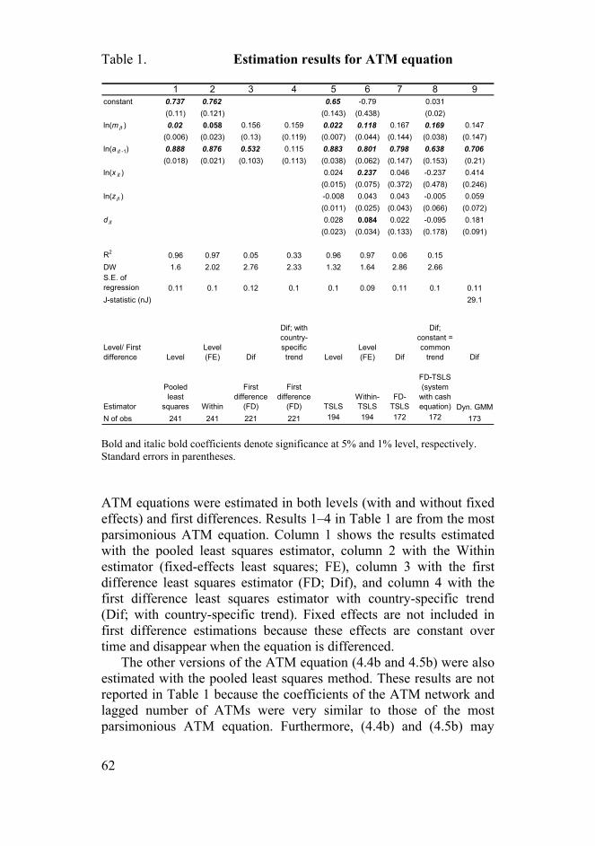
62

Table 1. Estimation results for ATM equation

1 2 3 4 5 6 7 8 9constant 0.737 0.762 0.65 -0.79 0.031

(0.11) (0.121) (0.143) (0.438) (0.02)ln(m jt ) 0.02 0.058 0.156 0.159 0.022 0.118 0.167 0.169 0.147

(0.006) (0.023) (0.13) (0.119) (0.007) (0.044) (0.144) (0.038) (0.147)ln(a jt -1) 0.888 0.876 0.532 0.115 0.883 0.801 0.798 0.638 0.706

(0.018) (0.021) (0.103) (0.113) (0.038) (0.062) (0.147) (0.153) (0.21)ln(x jt ) 0.024 0.237 0.046 -0.237 0.414

(0.015) (0.075) (0.372) (0.478) (0.246)ln(z jt ) -0.008 0.043 0.043 -0.005 0.059

(0.011) (0.025) (0.043) (0.066) (0.072)d jt 0.028 0.084 0.022 -0.095 0.181

(0.023) (0.034) (0.133) (0.178) (0.091)

R2 0.96 0.97 0.05 0.33 0.96 0.97 0.06 0.15DW 1.6 2.02 2.76 2.33 1.32 1.64 2.86 2.66S.E. of regression 0.11 0.1 0.12 0.1 0.1 0.09 0.11 0.1 0.11J-statistic (nJ) 29.1

Level/ First difference Level

Level (FE) Dif

Dif; with country-specific trend Level

Level (FE) Dif

Dif; constant = common

trend Dif

Estimator

Pooled least

squares Within

First difference

(FD)

First difference

(FD) TSLSWithin-TSLS

FD-TSLS

FD-TSLS (system

with cash equation) Dyn. GMM

N of obs 241 241 221 221 194 194 172 172 173 Bold and italic bold coefficients denote significance at 5% and 1% level, respectively. Standard errors in parentheses. ATM equations were estimated in both levels (with and without fixed effects) and first differences. Results 1–4 in Table 1 are from the most parsimonious ATM equation. Column 1 shows the results estimated with the pooled least squares estimator, column 2 with the Within estimator (fixed-effects least squares; FE), column 3 with the first difference least squares estimator (FD; Dif), and column 4 with the first difference least squares estimator with country-specific trend (Dif; with country-specific trend). Fixed effects are not included in first difference estimations because these effects are constant over time and disappear when the equation is differenced. The other versions of the ATM equation (4.4b and 4.5b) were also estimated with the pooled least squares method. These results are not reported in Table 1 because the coefficients of the ATM network and lagged number of ATMs were very similar to those of the most parsimonious ATM equation. Furthermore, (4.4b) and (4.5b) may

63

include the endogenous problem. Cash in circulation may affect the number of ATMs and the number of ATMs may affect cash in circulation. Therefore, we estimated (4.4b) and (4.5b) also with the pooled TSLS method, as reported in Table 1, columns 5–7. Column 5 gives the estimation results with the TSLS estimator, column 6 with the Within-TSLS estimator (with fixed effects), and column 7 with the first difference TSLS estimator (FD-TSLS; Dif). In the estimations, we used right-hand side variables, two-period lagged dependent variable and one-period lagged cash as instruments. Furthermore, we included the deposit interest rate in the instruments because it may affect both cash in circulation and card usage. The one-period lagged value of card payments was also included in the instruments. The number of ATM transactions could also be used as an instrument, but these data are not available for all countries (eg for Denmark the data on ATM transactions are available only for one year). To sum up, the instruments for the TSLS estimations reported in columns 5–6 are: constant, ln(mjt), ln(xjt–1), ln(zjt), ln(zjt–1), ln(ajt–2), djt and ijt. The instruments for the system TSLS estimation in first differences in column 7 are: ∆ln(mjt), ∆ln(xjt–1), ∆ln(zjt), ∆ln(zjt–1), ∆ln(ajt–2), ∆djt and ∆ijt. Column 8 includes the results of system estimation of ATM and cash equations. The system TSLS estimation includes trend in both the ATM and cash equations. In other words, results in column 8 are estimated with the first difference TSLS estimator with a common trend for all countries (Dif; with common trend). The instrument set used in column 8 is: constant, ∆ln(mjt), ∆ln(xjt–1), ∆ln(zjt), ∆ln(zjt–1), ∆ln(ajt–2), ∆ln(yjt), ∆ijt and ∆djt. Column 9 presents the results of the dynamic panel data GMM estimation (Arellano-Bond 1-step estimation); the instrument set used in that estimation is the following: ∆ln(mjt), ∆ln(mjt–1), ∆ln(xjt–1), ∆ln(xjt–2), ∆ln(zjt), ∆ln(zjt–1), ∆ln(ajt–2), ∆ln(ajt–3), ∆ijt and ∆djt. Due to the lack of data, we instrumented the lagged dependent variable only with two and three lags. Furthermore, cash was instrumented with one and two lags. Otherwise, the independent variables are assumed to be exogenous. The estimation results in Table 1 indicate that the number of ATM networks has a positive sign, as expected. Moreover, the number of ATM networks is a statistically significant variable in estimations 1, 2, 5, 6 and 8. As seen, level estimations, with and without fixed effects, and the system estimation of ATM and cash equations with trend indicate such a result. However, other first difference estimation results indicate that the number of ATM networks is not a statistically significant variable. We report for estimations 1–7 and 9 the adjusted t-values calculated using the White diagonal method, which is one of

64

the White coefficient covariance methods. The ordinary coefficient covariance method indicates remarkably higher t-values and, according to those values, the ATM network is statistically significant also in first difference estimations. The coefficient of the one-period lagged dependent variable is positive and statistically significant in almost all estimations. Only the result of estimation 4, ie using the most parsimonious model with country-specific trend, indicates that the one-period lagged dependent variable is statistically insignificant. The reason behind this is that country-specific trends take the explanatory power of other variables. Country-specific trends are positive and significant for 18 countries. Only for Finland and Norway is the coefficient of trend variable insignificant. Moreover, Finland is the only country with a negative sign for the country-specific trend. One reason for this may be that the development of payment systems is at a higher level in Finland than in other countries. Table 1 also shows that the coefficient of cash in circulation is usually positive but insignificant. Furthermore, estimation results show that the value of card payments is not a statistically significant variable. However, the sign of card payments should be negative according to our hypothesis. The positive sign indicated by some of the estimations may be due to the dual nature of payment cards. People can usually withdraw cash with same payment cards with which they pay for transactions. Increased card payments are typically related to an increased number of payment cards, which makes cash withdrawals easier. Thus increasing card payments may increase the number of ATM withdrawals and hence the number of ATMs. (4.4a), (4.4b), (4.5a) and (4.5b) are the partial adjustment models that give the short-run effects, and long-run effects can be calculated based on these results. In other words, the coefficients reported in Table 1 are short-run effects. For instance, based on the results in column 1, a 1% decrease in the number of ATM networks would reduce the number of ATMs per million inhabitants by ca 0.02% in the short-run. In the long-run, the coefficient is 0.02/(1 – 0.888) = 0.2. This means that in the long-run a 1% decrease in the number of ATM networks would reduce the number of ATMs per million inhabitants by 0.2%. In other words, the long-run elasticity of the number of ATMs with respect to the number of ATM networks is 0.2. The long-run elasticities calculated on the basis of the results reported in columns 1–9 are between 0.18 and 0.83. As seen, the short-run elasticities of the number of ATMs with respect to the number of ATM networks are lowest in results reported in columns 1 and 5. One obvious reason for this is that these

65

estimations are biased. Therefore, we have to include the fixed effects in the level estimation or estimate the ATM equation in first differences, as discussed in Section 4.3.1. Comparing these results reveals that country-specific effects correlate negatively with ATM networks. For instance, in the Nordic countries, the numbers of ATMs per inhabitant are small and there is only one ATM network in each country. On the contrary, there are dozens of ATM networks eg in the USA and Canada and the numbers of ATMs per inhabitant are high. Moreover, not all these networks are compatible. We did some other estimations. Based on our theoretical discussion, population and the value of GDP per capita could also be included in the ATM equation. Intuitively, the number of ATMs depends positively on the number of inhabitants if banks aim at offering a high level of service. The number of ATMs may also depend positively on GDP per capita, as this is an approximate of the value of transactions per capita. We added population and GDP per capita in estimations 1–9, and the results were similar to those reported in Table 1. The coefficient of the number of ATM networks was still positive, and the additional variables were statistically significant only in estimation 3. Based on these model specifications, the results reported in Table 1 seem to be robust. An extensive number of diagnostic tests were performed on the ATM equation estimations. Results of these tests can be summarised as follows: 1) Group unit root tests on residuals for equations 1–7, as well as panel unit root tests for equations 8–9, indicate that the residuals are stationary in levels. 2) According to the Jarque-Bera test, the null hypothesis that residuals are normally distributed cannot be rejected in most cases. Furthermore, the figures and statistics for residuals indicate that mean and median are roughly zero. 3) The test for equality of variances (estimations 1–7) rejects the null hypothesis that variances of residuals of various countries are the same. In other words, there seems to be groupwise heteroskedasticity in residuals. In contrast, residuals for estimations 8–9 seem to be homoskedastic. 4) Durbin-Watson test indicates some serial correlation. However, the Durbin-Watson test may not be suitable for the ATM equation because we have included the lagged dependent variable as an explanatory variable (eg Pindyck and Rubinfeld 1998, p. 165). Moreover, the Durbin-Watson test cannot be used with dynamic GMM estimation21. Correlogram Q-statistics of residuals indicate that 21 In Arellano-Bond estimations, m1 and m2 autocorrelation tests could be used. We were not able to perform these tests with the software used in the estimations. However, reported t-statistics are adjusted via the White diagonal coefficient covariance method.

66

the null hypothesis of no serial correlation needs to be rejected for some countries. Residuals of some countries also seem to be correlated based on the pairwise correlation matrices. We have reported adjusted t-statistics in estimations 1–7 and 9 using the White diagonal method. If we use the ordinary covariance method instead, the t-statistics reported in Table 1 change somewhat, and the variable ATM network becomes statistically significant in all estimations. Furthermore, we tested the validity of the overidentifying restrictions22 in the dynamic panel data GMM estimation. According to the J-statistic, the null hypothesis that the overidentifying restrictions are satisfied cannot be rejected, suggesting that we have used a proper instrument set. 4.3.3 Results of cash equation estimations

Estimation results for the cash equation in levels, with and without fixed effects, and in first differences are reported in Table 2. The cash equation was estimated with same estimation methods as the ATM equation in Section 4.3.2. Column 10 shows the results estimated with the pooled least squares estimator, column 11 with the Within estimator (fixed-effects least squares; FE), column 12 with the first difference least squares estimator (FD; Dif), and column 13 with the first difference least squares estimator with country-specific trend (Dif; with country-specific trend). The pooled TSLS method was used because there may be an endogeneity problem. As discussed above, the number of ATMs may affect cash in circulation, and vice versa. Column 14 shows the estimation results with TSLS estimator, column 15 with the Within-TSLS estimator (with fixed effects), and column 16 with the first difference TSLS estimator (FD-TSLS; Dif). Column 17 includes the results of system estimation of the ATM and cash equations, with trend included in both. In other words, results in column 17 are estimated with the first difference TSLS estimator with a common trend for all countries (Dif; with common trend). Column 18 gives the estimation results for the dynamic panel data GMM estimation (Arellano-Bond 1-step estimation).

22 For example, Arellano (2003) p. 192–197 discusses the testing of overidentifying restrictions.

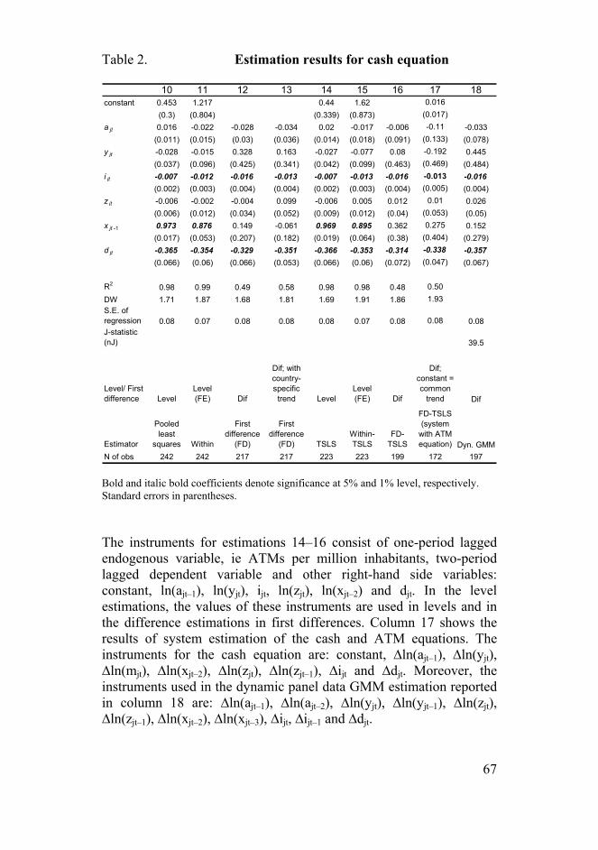
67

Table 2. Estimation results for cash equation

10 11 12 13 14 15 16 17 18constant 0.453 1.217 0.44 1.62 0.016

(0.3) (0.804) (0.339) (0.873) (0.017)a jt 0.016 -0.022 -0.028 -0.034 0.02 -0.017 -0.006 -0.11 -0.033

(0.011) (0.015) (0.03) (0.036) (0.014) (0.018) (0.091) (0.133) (0.078)y jt -0.028 -0.015 0.328 0.163 -0.027 -0.077 0.08 -0.192 0.445

(0.037) (0.096) (0.425) (0.341) (0.042) (0.099) (0.463) (0.469) (0.484)i jt -0.007 -0.012 -0.016 -0.013 -0.007 -0.013 -0.016 -0.013 -0.016

(0.002) (0.003) (0.004) (0.004) (0.002) (0.003) (0.004) (0.005) (0.004)z jt -0.006 -0.002 -0.004 0.099 -0.006 0.005 0.012 0.01 0.026

(0.006) (0.012) (0.034) (0.052) (0.009) (0.012) (0.04) (0.053) (0.05)x jt -1 0.973 0.876 0.149 -0.061 0.969 0.895 0.362 0.275 0.152

(0.017) (0.053) (0.207) (0.182) (0.019) (0.064) (0.38) (0.404) (0.279)d jt -0.365 -0.354 -0.329 -0.351 -0.366 -0.353 -0.314 -0.338 -0.357

(0.066) (0.06) (0.066) (0.053) (0.066) (0.06) (0.072) (0.047) (0.067)

R2 0.98 0.99 0.49 0.58 0.98 0.98 0.48 0.50DW 1.71 1.87 1.68 1.81 1.69 1.91 1.86 1.93S.E. of regression 0.08 0.07 0.08 0.08 0.08 0.07 0.08 0.08 0.08J-statistic (nJ) 39.5

Level/ First difference Level

Level (FE) Dif

Dif; with country-specific

trend LevelLevel (FE) Dif

Dif; constant = common

trend Dif

Estimator

Pooled least

squares Within

First difference

(FD)

First difference

(FD) TSLSWithin-TSLS

FD-TSLS

FD-TSLS (system

with ATM equation) Dyn. GMM

N of obs 242 242 217 217 223 223 199 172 197 Bold and italic bold coefficients denote significance at 5% and 1% level, respectively. Standard errors in parentheses. The instruments for estimations 14–16 consist of one-period lagged endogenous variable, ie ATMs per million inhabitants, two-period lagged dependent variable and other right-hand side variables: constant, ln(ajt–1), ln(yjt), ijt, ln(zjt), ln(xjt–2) and djt. In the level estimations, the values of these instruments are used in levels and in the difference estimations in first differences. Column 17 shows the results of system estimation of the cash and ATM equations. The instruments for the cash equation are: constant, ∆ln(ajt–1), ∆ln(yjt), ∆ln(mjt), ∆ln(xjt–2), ∆ln(zjt), ∆ln(zjt–1), ∆ijt and ∆djt. Moreover, the instruments used in the dynamic panel data GMM estimation reported in column 18 are: ∆ln(ajt–1), ∆ln(ajt–2), ∆ln(yjt), ∆ln(yjt–1), ∆ln(zjt), ∆ln(zjt–1), ∆ln(xjt–2), ∆ln(xjt–3), ∆ijt, ∆ijt–1 and ∆djt.

68

Almost all estimation results indicate that cash in circulation depends negatively on the number of ATMs. Only level estimations without fixed effects (columns 10 and 14) indicate the opposite. As discussed in Section 4.3.1, at least results obtained using the pooled least squares estimator and the TSLS estimator in levels without fixed effects may be biased. Therefore, it is obvious that the dependence between cash in circulation and number of ATMs is negative. However, the number of ATMs is not a statistically significant variable in these estimations. Furthermore, cash in circulation depends negatively on the deposit interest rate, as expected. The deposit interest rate is also a statistically significant variable in all estimations. The semi-elasticity of cash in circulation with respect to the deposit interest rate is ca –0.01 or –0.02 in the short-run. This means that if the deposit interest rate increases by one percentage point, cash in circulation decreases by 0.01%–0.02% in the short-run. The coefficient of the euro dummy is negative and statistically significant, as expected. The euro changeover led to a remarkable decrease in cash in circulation in all euro countries before year 2002. Coefficients of the variables GDP per population and value of card payments per population are not statistically significant. The coefficient of GDP per population differs as between level and difference estimations. Estimations in first differences indicate that cash in circulation depends positively on the GDP, as assumed. A positive relationship is a more reliable result because level estimations may be biased, as discussed in Section 4.3.1. Furthermore, the one-period lagged dependent variable is positive but not necessarily statistically significant. However, column 13 indicates a negative sign, which conflicts with expectations. This may be due to the country-specific trend, which varies considerably from country to country and weakens the explanatory power of other variables. The diagnostic tests of the cash equation in Table 2 indicate the following results: Residuals are stationary in levels, the null hypothesis of the Jarque-Bera that residuals are normally distributed cannot be rejected for most countries, and there is groupwise heteroskedasticity and correlation between the residuals of various countries. However, the residuals of estimations 17 and 18 indicate no heteroskedasticity or correlation in residuals. We also estimated the cash equation using the ordinary coefficient covariance method instead of the White diagonal method. Based on these estimations, there were no significant changes in the results. Furthermore, the J-statistic for the cash equation estimated with the dynamic panel data GMM estimation method indicates that the null hypothesis of the overidentifying restrictions being satisfied cannot be rejected.

69

We also estimated columns 14–18 with additional instruments. The inflation rate may well influence cash in circulation. Moreover, the number of EFTPOS terminals may affect both the value of card payments (positively) and cash in circulation (negatively) because a high density of EFTPOS terminals enables more convenient use of payment cards. Therefore, we included the inflation rate and the number of EFTPOS terminals in the instrument list for estimations 14–18. These changes did not have any notable effect on the results. 4.4 Discussion of estimation results

The topic of this study includes two main questions: 1) How does ATM network market structure and changes in it affect the availability of ATMs and cash withdrawal services? 2) How does this affect cash usage? Firstly, the estimation results indicate that a decrease in the number of ATM networks leads to a decrease in the number of ATMs. In other words, the monopolisation of ATM network market structure seems to lead to a reduced service level, as expected. Secondly, the influence of the number of ATMs on cash in circulation is ambiguous. In this section, we discuss the main findings of the estimations. The sign of the ATM network is positive in all versions of the ATM equation estimations. In the short-run, the elasticity is 0.02–0.17 and in the long-run 0.18–0.83 (Table 3). Table 3. Elasticity of number of ATMs with respect to number of ATM networks

Estimation results (column number) Short-run elasticity Long-run elasticity

1 0.02 0.182 0.06 0.473 0.16 0.334 0.16 0.185 0.02 0.196 0.12 0.597 0.17 0.838 0.17 0.479 0.15 0.50

Bold and italic bold coefficients denote significance at 5% and 1% level, respectively.

70

The effects of changes in the number of ATM networks on the number of ATMs are greater when the degree of monopolisation increases. In other words, if the number of ATM networks decreases from 10 to 9 networks, this is a 10% decrease in networks. For example, according to the results of the dynamic panel data estimation (estimation 9), this would imply a 1.5% decrease in the number of ATMs per million inhabitants in the short-run and a 5% decrease in the long-run. However, if the market arrives at monopoly from duopoly, ie the number of ATM networks decreases from two to one, this is a 50% decrease in the number of networks. This leads to a 7.5% decrease in the number of ATMs in the short-run and a 25% decrease in the long-run. This would be quite a remarkable decrease in the number of ATMs. For instance, in Finland, the number of ATMs decreased by one-fifth in 1993–1995, as the number of ATM networks decreased from three to one. On the other hand, the decrease in the number of ATMs has continued and we could assume that the decrease in the number of ATM networks affects ATMs for a longer period than just one year. If the number of ATM networks decreases at the end of the year, all effects on the number of ATMs will obviously not be realised during the same year. However, in order to minimise the number of explanatory variables, we did not add lagged independent variables to the right-hand side of the equations. Table 3 indicates that the short-run elasticities of the number of ATMs with respect to the number of ATM networks are lowest for results 1 and 5. These results are from level estimations without fixed effects. Thus these estimations obviously are biased. The long-run elasticities of estimations 1 and 5 are also biased because the coefficient of the lagged dependent variable is biased, as well. These results suggest that country-specific effects correlate negatively with ATM networks, as discussed in Section 4.3.2. Therefore, the level estimations with fixed effects or estimations in first differences are more reliable than results 1 and 5.

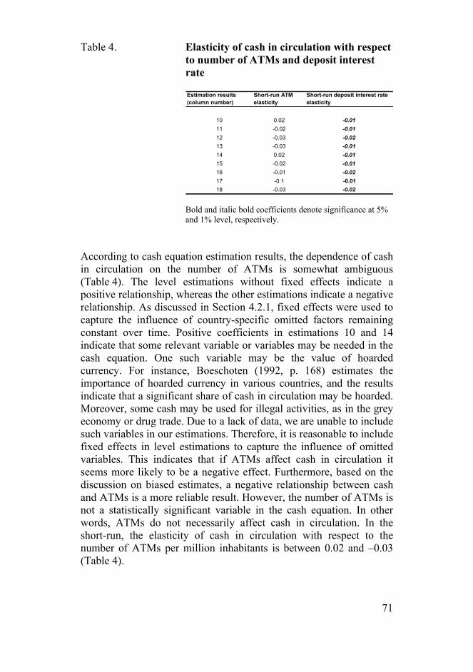
71

Table 4. Elasticity of cash in circulation with respect to number of ATMs and deposit interest rate

Estimation results (column number)

Short-run ATM elasticity

Short-run deposit interest rate elasticity

10 0.02 -0.0111 -0.02 -0.0112 -0.03 -0.0213 -0.03 -0.0114 0.02 -0.0115 -0.02 -0.0116 -0.01 -0.0217 -0.1 -0.0118 -0.03 -0.02

Bold and italic bold coefficients denote significance at 5% and 1% level, respectively. According to cash equation estimation results, the dependence of cash in circulation on the number of ATMs is somewhat ambiguous (Table 4). The level estimations without fixed effects indicate a positive relationship, whereas the other estimations indicate a negative relationship. As discussed in Section 4.2.1, fixed effects were used to capture the influence of country-specific omitted factors remaining constant over time. Positive coefficients in estimations 10 and 14 indicate that some relevant variable or variables may be needed in the cash equation. One such variable may be the value of hoarded currency. For instance, Boeschoten (1992, p. 168) estimates the importance of hoarded currency in various countries, and the results indicate that a significant share of cash in circulation may be hoarded. Moreover, some cash may be used for illegal activities, as in the grey economy or drug trade. Due to a lack of data, we are unable to include such variables in our estimations. Therefore, it is reasonable to include fixed effects in level estimations to capture the influence of omitted variables. This indicates that if ATMs affect cash in circulation it seems more likely to be a negative effect. Furthermore, based on the discussion on biased estimates, a negative relationship between cash and ATMs is a more reliable result. However, the number of ATMs is not a statistically significant variable in the cash equation. In other words, ATMs do not necessarily affect cash in circulation. In the short-run, the elasticity of cash in circulation with respect to the number of ATMs per million inhabitants is between 0.02 and –0.03 (Table 4).

72

Earlier empirical research has also produced contradictory results about the influence of ATMs on cash in circulation. The effects of ATMs on cash usage are ambiguous also based on our theoretical discussion in Section 3. Moreover, the euro conversion may affect our estimations results. The value of cash in all euro countries decreased considerably before the changeover to euro at the beginning of 2002. This transition may have affected our results even though the euro dummy variable was included in the estimations. The euro dummy is negative and statistically significant in all versions of the cash equation estimations. Furthermore, data on cash have not been available for single euro countries since 2002. The deposit interest rate is a statistically significant variable in all estimations and it has a negative sign, as expected. If the deposit interest rate increases, the opportunity cost of cash holdings increases. Therefore, cash in circulation was presumed to decrease. According to all estimations, the coefficient of the deposit interest rate is (-0.01)– (–0.02) in the short-run (Table 4). This is the semi-elasticity because we did not use the logarithm transformation of the deposit interest rate. In other words, a one percentage point increase in the deposit interest rate reduces cash in circulation per population by 0.01% in the short-run. Compared to earlier empirical results, these interest rate elasticities are of similar sign and fairly similar in size. For instance, Drehmann et al (2002) report the interest rate elasticity of cash demand to be between (–0.003)–(–0.006) and Snellman et al (2000) report the interest rate elasticity of currency holdings per person to be (–0.24). Furthermore, Attanasio et al (2002) find an interest rate elasticity of (–0.59) for the demand for currency of those who have a bank account and ATM card. According to the same study, the interest rate elasticity of the demand for currency for those with bank account but without ATM card is found to be (–0.27). Thus our results are well within the range reported by several other studies.

73

5 Conclusions This study analysed the effects of ATM network market structure on the number of ATMs and cash usage. The influence of cash distribution technology and changes in it are of the essence for central banks, as seigniorage is based on cash usage. At the same time, the development of retail payments and the usage of payment instruments are relevant questions for many other parties, such as banks and consumers. Section 2 argued that the dependence between ATM network market structure and the number of ATMs has not been thoroughly analysed. Furthermore, based on the earlier literature, the effects of ATMs on cash in circulation are ambiguous. In Section 3, we theoretically analysed the influence of ATM network market structure on the number of ATMs and on the demand for money. Both the consumer’s and the bank’s optimisation problems were analysed in order to determine the optimal number of ATMs and the optimal value of cash holdings. In addition to the theoretical analysis, in Section 4 we tested empirically the hypotheses formed based on the theoretical discussion. A unique data set on 20 countries used in estimations was combined from various data sources. We estimated the ATM and cash equations using various estimation methods, all of which produced results quite similar to those of our research questions. The estimation results support the hypothesis that a reduction in the number of ATM networks decreases the number of ATMs. In other words, the monopolisation of ATM network market structure leads to a lower service level. This is in line with our theoretical discussion and with the industrial organisation literature. Furthermore, our estimation results indicate that the influence of the number of ATMs on cash in circulation and seigniorage is somewhat ambiguous but more likely negative than positive. Also, based both on our theoretical discussion and on the earlier empirical work, the effect of the number of ATMs on cash usage seems to be somewhat contradictory. In addition to these main results, the relationship between deposit interest rate and cash in circulation is negative and statistically significant in all our estimations, as expected based on the earlier literature. Lack of data often restricts empirical research on payment systems. The development of payment systems has been very rapid over the past few decades and, for example, the first ATMs were installed in the 1960s or 1970s in many of the countries analysed in this study. However, harmonised data on various countries have been

74

available only since 1988 or 1990, which leads to a short observation period. Also, the euro conversion in 2002 affected cash in circulation in the euro countries. Especially during the year 2001, cash in circulation decreased considerably in these 12 countries. Moreover, the value of euros in circulation has not been available for individual euro countries since 2002, as only the total value of euros in circulation has been published. 5.1 Policy discussion

Our main result, ie that the monopolisation of ATM networks leads to a decreased number of ATMs, may have various policy implications. On the one hand, decreasing competition may have harmful consequences from the consumers’ point of view. The availability of ATM services may diminish if the monopoly decides to reduce the number of ATMs. Furthermore, it may be easier for a monopoly ATM service provider to increase the fees for cash withdrawals. There are some countries in which cash withdrawals are free of charge. In such cases, the monopoly ATM service provider may have incentives to start charging a fee for cash withdrawals. On the other hand, maintaining many parallel ATM networks is expensive. At least in a small, sparsely inhabited country this cost may be substantial. The main question is who pays the expenses of cash maintenance. Concerning cash usage, the role of the central bank is of the essence. The maintenance of currency is one of the responsibilities of central banks. Cash is the only legal tender, and central banks have a monopoly in issuing currency in circulation. They have to ascertain the sufficiency of cash. As the seigniorage of central banks is based on cash usage, changes and developments in payment systems and especially in cash usage are of importance to them. Furthermore, central banks should promote the efficiency of payment systems23. Payment instruments are part of the overall payment system, and cash usage seems to be quite an inefficient payment instrument compared

23 The task of central banks in promoting efficient payment systems is mentioned in the law. Koskenkylä (2003, p. 313–314) discusses this as follows: “According to Article 22 of the Statute of the European System of Central Banks, the European Central Bank and the national central banks may provide the actual systems while the ECB may issue regulations on the maintenance of efficient and stable payment systems…” Furthermore, “according to Article 3 of the Act on the Bank of Finland, one of the Bank’s main tasks is to contribute to maintaining the reliability and efficiency of payment and other financial systems and to take part in the development of these systems.”

75

to electronic payment methods. However, efficiency in this context should be regarded as social efficiency, the analysis of which has not been the object of this paper. Furthermore, cash is the only anonymous payment instrument. Even if the legal transactions demand for cash decreases considerably or ceases totally, cash may still be demanded eg for grey or black economy transactions. Moreover, some cash is used for precautionary or speculative purposes, and some currency may be used outside the country or currency area. An important aspect of maintenance of cash supply is to decide on the distribution of notes to people who prefer cash payments. All citizens should have access to cash distributing services. For instance, in Finland, the major part of cash is withdrawn at ATMs. However, ATM networks are not maintained by central banks but typically by banks or by separate bank-owned companies. Cash maintenance generates costs to banks, and so, they may have incentives to reduce cash usage. One efficient way to do this is to reduce the number of ATMs or to start pricing cash withdrawal services. Banks have already encouraged their customers to increase the use of electronic means of payment via price incentives. Both the number of payment cards and the value and volume of card payments have been increasing during the last ten or fifteen years. Banks may also have incentives to reduce the number of bank branches or at least to concentrate on customer services other than routine ones like cash withdrawals. The countries discussed in this paper have different payment systems. Some have more highly developed payment systems than others, eg the use of cheques versus payment cards varies considerably across countries. The observation period 1988–2003 is short, and payment systems in various countries are developing all the time. It is interesting to consider whether this development will lead to homogeneous payment systems in all countries. For instance, there is a Single Euro Payment Area (SEPA) project in the euro area, having many common goals for payment systems development in the EU countries (eg Koskenkylä 2004, ch. 6). To achieve the goals of SEPA, all parties need to enhance the development of the payment systems and co-operate with each other. The development of the payment sector challenges both the market side and the authorities. Cash usage and ATM network market structure may change as the payment system sector develops. It would be interesting to replicate this study after 20 years to test whether the main results remain the same.

76

5.2 Topics for further research

The market structure of ATM networks and its effects on cash usage and seigniorage are important questions from many stakeholders’ points of view. One challenge for future research would be to thoroughly analyse the technology development of the payment systems and its influence on ATM network market structure and cash usage. Payment systems vary across countries, and in some countries people use more electronic payment instruments more than in others. For instance, in the Nordic countries, cash in circulation is low, and the use of payment cards and electronic credit transfers, eg Internet banking, is popular. Furthermore, cheques have vanished from retail sales, and the infrastructure is highly developed. Payments are electronically transmitted and, for example, the number of EFTPOS terminals per capita is very high. A second topic for future research would be to adapt the equations estimated in this paper to a wider group of countries. There may be some problems due to a lack of data, but at least the ten new EU countries, which joined the EU in May 2004, could be included in the data set. Payment systems have been developing very rapidly in most of these countries over the past decade, so that the results may differ compared to the 20 countries analysed in this paper. A third contribution to the discussion would be to elaborate the spatial model presented in this paper eg by explicitly including the effects of various market structures. This would enable comparative analysis under monopoly, duopoly, oligopoly and perfect competition. Furthermore, other obvious features of the ATM network market, such as network externalities and compatibility and incompatibility of ATM networks, could possibly be included in the model. To conclude, the ATM network market structure has a significant influence on the number of ATMs. Changes in market structure potentially affect both banks and central banks. These changes also have an influence on each individual consumer and his or her payment habits, at least in the long run. We have seen remarkable changes in payment habits during the last few decades. This development will continue and will present new challenges for future research on payment systems.

77

References Angelini, P – Hendry, D – Rinaldi, R (1994) An Econometric

Analysis of Money Demand in Italy. Temi di discussione del Servizio Studi, No. 219, Banda d’Italia.

Arellano, M (2003) Panel Data Econometrics. Advanced texts in

econometrics, Oxford University Press, Oxford. Arellano, M – Bond, S (1991) Some Tests of Specification for Panel

Data: Monte Carlo Evidence and an Application to Employment Equations. The Review of Economic Studies, Vol. 58, No. 2, 277–297.

Association for Payment Clearing Services (2004) ATM Survey

2004. Attanasio, O – Guiso, L – Jappelli, T (2002) The Demand for

Money, Financial Innovation, and the Welfare Cost of Inflation: An Analysis with Household Data. Journal of Political Economy, Vol. 110, No. 2, 317–351.

Avery, R (1996) Comment on Cash, Paper, and Electronic

Payments: A Cross-Country Analysis. Journal of Money, Credit and Banking, Vol. 28, No. 4, Part 2, 940–941.

Baker, D (1995) Shared ATM Networks – The Antitrust

Dimension. Federal Reserve Bank of St. Louis Review, November/December 1995, 5–17.

Baltagi, B (2001) Econometric Analysis of Panel Data. John Wiley

& Sons, Chichester. Balto, D (1995) Payment Systems and Antitrust: Can the

Opportunities For Network Competition Be Recognized? Federal Reserve Bank of St. Louis Review, November/December 1995, 19–40.

Bank for International Settlements (1985) Payment Systems in

Eleven Developed Countries.

78

Bank for International Settlements (1989) Payment Systems in Eleven Developed Countries.

Bank for International Settlements (1993) Payment Systems in the

Group of Ten Countries. Bank for International Settlements (2003) Payment and Settlement

Systems in Selected Countries. Bank of Finland (1993) Payment and Settlement Systems in

Finland. Bank of Finland publications A:88. Barton, D – Sherman, R (1984) The Price and Profit Effects of

Horizontal Merger: A Case Study. The Journal of Industrial Economics, Vol. 33, No. 2, 165–177.

Baumol, W (1952) The Transactions Demand for Cash: An

Inventory Theoretic Approach. The Quarterly Journal of Economics, Vol. 66, No. 4, 545–556.

Boeschoten, W (1992) Currency Use and Payment Patterns.

Financial and Monetary Policy Studies, 23. Kluwer Academic Publishers, Dordrecht.

Boeschoten, W (1998) Cash Management, Payment Patterns and

the Demand for Money. De Economist 146, No. 1, 117–142. Bolt, W (2003) Retail payments in the Netherlands: Some facts

and some theory. Research Memorandum WO No. 722, De Nederlandsche Bank.

Bolt, W – Tieman, A (2003) Pricing Debit Card Payment Services:

An IO Approach. IMF Working Paper 202/2003. Carlton, D – Frankel, A (1995) Antitrust and Payment

Technologies. Federal Reserve Bank of St. Louis Review, November/December 1995, 41–54.

Chakravorti, S (2003) Theory of Credit Card Networks: A Survey

of the Literature. Review of Network Economics, Vol. 2, Issue 2, 50–68.

79

Chakravorti, S – Roson, R (2004) Platform Competition in Two-Sided Markets: The Case of Payment Networks. Working Paper 2004–09, Federal Reserve Bank of Chicago.

Chiang, A (1984) Fundamental Methods of Mathematical

Economics. McGraw-Hill Book Co., Singapore. Croft, E – Spencer, B (2003) Fees and Surcharging in Automatic

Teller Machine Networks: Non-Bank ATM Providers versus Large Banks. Working Paper 9883, NBER Working Paper Series.

Davidson, R – MacKinnon, J (2004) Econometric Theory and

Methods. Oxford University, New York. Dranove, D – Gandal, N (2003) The DVD vs. DIVX Standard War:

Empirical Evidence of Network Effects and Preannouncement Effects. Journal of Economics and Management Strategy, 12, 363–386.

Drehmann, M – Goodhart, C (2000) Is Cash Becoming

Technologically Outmoded? Or Does it Remain Necessary to Facilitate “Bad Behaviour”? An Empirical Investigation into the Determinants of Cash Holdings. Discussion Paper 358, LSE Financial Markets Group, Discussion Paper Series.

Drehmann, M – Goodhart, C – Krueger, M (2002) The challenges

facing currency usage: will the traditional transaction medium be able to resist competition from the new technologies? Economic Policy, Vol. 17, No. 34, 195–227.

Duca, J – Whitesell, W (1995) Credit Cards and Money Demand: A

Cross-sectional Study. Journal of Money, Credit and Banking, Vol. 27, No. 2, 604–623.

Duca, J – VanHoose, D (2004) Recent developments in

understanding the demand for money. Journal of Economics and Business, 56, 247–272.

Economides, N (1989) Desirability of Compatibility in the Absence

of Network Externalities. The American Economic Review, Vol. 79, No. 5, 1165–1181.

80

Economides, N (1996) Network externalities, complementarities, and invitations to enter. European Journal of Political Economy, Vol. 12, 211–233.

EMEAP (Executives’ Meeting of East Asia-Pacific Central Banks and

Monetary Authorities) (2002) Payment Systems in EMEAP Economies.

Emmons, W – Prager, R (1997) The Effects of Market Structure

and Ownership on Prices and Service Offerings in the U.S. Cable Television Industry. The RAND Journal of Economics, Vol. 28, No. 4, 732–750.

European Central Bank (2001) Payment and securities settlement

systems in the European Union (Blue Book). European Monetary Institute (1996) Payment systems in the

European Union. Farrell, J – Saloner, G (1985) Standardization, Compatibility, and

Innovation. The RAND Journal of Economics, Vol. 16, No. 1, 70–83.

Farrell, J – Saloner, G (1986) Installed Base and Compatibility:

Innovation, Product Preannouncements, and Predation. The American Economic Review, Vol. 76, No. 5, 940–955.

Finnish Bankers’ Association (2004) Statistical Data on Banks’

Payment Systems in Finland 1994–2003. Frame, W – White, L (2004) Empirical Studies of Financial

Innovation: Lots of Talk, Little Action? Journal of Economic Literature, Vol. XLII, 116–144.

Gandal, N (1994) Hedonic Price Indexes for Spreadsheets and an

Empirical Test for Network Externalities. The RAND Journal of Economics, Vol. 25, No. 1, 160–170.

Gandal. N – Kende, M – Rob, R (1999) The Dynamics of

Technological Adoption in Hardware/Software Systems: The Case of Compact Disc Players. Discussion Paper No. 2078, Centre for Economic Policy Research.

81

Gans, J – King, S (2003) Approaches to Regulating Interchange Fees in Payment Systems. Review of Network Economics, Vol. 2, Issue 2, 125–145.

Goodhart, C – Krueger, M (2001) The Impact of Technology on

Cash Usage. Discussion Paper 374, LSE Financial Markets Group, Discussion Paper Series.

Gowrisankaran, G – Holmes, T (2002) Do Mergers Lead to

Monopoly in the Long Run? Results from the Dominant Firm Model. NBER Working Paper No. 9151.

Greene, W (2000) Econometric Analysis. Prentice-Hall International,

Upper Saddle River, New Jersey. Guibourg, G – Segendorf, B (2004) Do Prices Reflect Costs? A

study of the price- and cost structure of retail payment services in the Swedish banking sector 2002. Working Paper 172, Sveriges Riksbank, Working Paper Series.

Guthrie, G – Wright, J (2003) Competing Payment Schemes.

Working Paper No. 0311, National University of Singapore, Department of Economics.

Hancock, D – Humphrey, D (1998) Payment transactions,

instruments, and systems: A survey. Journal of Banking & Finance 21, 1573–1624.

Hancock, D – Humphrey, D – Wilcox, J (1999) Cost reductions in

electronic payments: The roles of consolidation, economies of scale, and technical change. Journal of Banking & Finance, 23, 391–421.

Hannan, T – McDowell, J (1984a) The Determinants of Technology

Adoption: The Case of the Banking Firm. The RAND Journal of Economics, Vol. 15, No. 3, 328–335.

Hannan, T – McDowell, J (1984b) Market Concentration and the

Diffusion of New Technology in the Banking Industry. The Review of Economics and Statistics, Vol. 66, No. 4, 686–691.

82

Hannan, T – McDowell, J (1987) Rival Precedence and the Dynamics of Technology Adoption: An Empirical Analysis. Economica, New Series, Vol. 54, No. 214, 155–171.

Hannan, T – McDowell, J (1990) The Impact of Technology

Adoption on Market Structure. The Review of Economics and Statistics, Vol. 72, No. 1, 164–168.

Hannan, T – Kiser, E – Prager, R – McAndrews, J (2003) To

Surcharge or not to Surcharge: an Empirical Investigation of ATM Pricing. The Review of Economics and Statistics, 85(4), 990–1002.

Hausman, J – Leonard, G – Tirole, J (2003) On nonexclusive

membership in competing joint ventures. The RAND Journal of Economics, Vol. 34, No. 1, 43–62.

Hester, D – Calcagnini, G – De Bonis, R (1999) Competition

through Innovation: ATMs in Italian Banks. Working Paper No. 27, University of Wisconsin Madison – Social Systems.

Hirvonen, J – Virén, M (1996a) Käteisrahan käyttö suomalaisissa

yrityksissä. Suomen Pankin tutkimuksia A:97. Hirvonen, J – Virén, M (1996b) The use of cash in Finnish business

firms. Bank of Finland Bulletin, No. 3, 3–9. Horn, H – Persson, L (2001) Endogenous mergers in concentrated

markets. International Journal of Industrial Organization, 19, 1213–1244.

Horvitz, P (1996) ATM Surcharges: Their Effect on Competition

and Efficiency. Journal of Retail Banking Services, Vol. XVIII, No. 3, 57–62.

Hsiao, C (2003) Analysis of Panel Data. Econometric Society

monographs, Cambridge University Press, Cambridge. Humphrey, D (1994) Delivering Deposit Services: ATMs Versus

Branches. Federal Reserve Bank of Richmond Economic Quarterly, Vol. 80, 59–81.

83

Humphrey, D – Pulley, L – Vesala, J (1996) Cash, Paper, and Electronic Payments: A Cross-Country Analysis. Journal of Money, Credit and Banking, Vol. 28, No. 4, Part 2, 914–939.

Humphrey, D – Kim, M – Vale, B (1998) Realizing the Gains from

Electronic Payments: Costs, Pricing and Payment Choice. Arbeidsnotat 1/1998, Norges Bank.

Humphrey, D – Willesson, M – Bergendahl, G – Lindblom, T (2003a)

Cost Savings from Electronic Payments and ATMs in Europe. Working Paper No. 03-16, Federal Reserve Bank of Philadelphia.

Humphrey, D – Willesson, M – Lindblom, T – Bergendahl, G (2003b)

What does it Cost to Make a Payment? Review of Network Economics, Vol. 2, Issue 2, 159–174.

Humphrey, D – Vale, B (2004) Scale economies, bank mergers, and

electronic payments: A spline function approach. Journal of Banking & Finance, 28, 1671–1696.

Japanese Bankers Association (2003) Payment Systems in Japan. Judson, R – Porter, R (2004) Currency demand by federal reserve

cash office: what do we know? Journal of Economics and Business, 56, 273–285.

Katz, M – Shapiro, C (1985) Network Externalities, Competition,

and Compatibility. The American Economic Review, Vol. 75, No. 3, 424–440.

Katz, M – Shapiro, C (1986a) Product Compatibility Choice in a

Market with Technological Progress. Oxford Economic Papers, New Series, Vol. 38, Supplement: Strategic Behaviour and Industrial Competition, 146–165.

Katz, M – Shapiro, C (1986b) Technology Adoption in the Presence

of Network Externalities. The Journal of Political Economy, Vol. 94, No. 4, 822–841.

Katz, M – Shapiro, C (1992) Product Introduction with Network

Externalities. The Journal of Industrial Economics, Vol. 40, No. 1, 55–83.

84

Katz, M – Shapiro, C (1994) Systems Competition and Network Effects. The Journal of Economic Perspectives, Vol. 8, No. 2, 93–115.

Kim, E – Singal, V (1993) Mergers and Market Power: Evidence

from the Airline Industry. The American Economic Review, Vol. 83, No. 3, 549–569.

Knittel, C – Stango, V (2004) Compatibility and Pricing with

Indirect Network Effects: Evidence from ATMs. Working Paper 10774, NBER Working Paper Series.

Koskenkylä, H (ed.) (2003) Finnish financial markets 2002. Bank of

Finland Studies A:105. Koskenkylä, H (ed.) (2004) Financial intergration. Bank of Finland

Studies A:108. Koskinen, J (2001) Yksityisasiakkaiden maksuliikepalvelujen hin-

noittelu Suomessa. Suomen Pankin keskustelualoitteita 12/2001. Krämer, W – Sonnberger, H (1986) The Linear Regression Model

Under Test. Physica-Verlag, Heidelberg. Laffont, J – Rey, P – Tirole, J (1998) Network Competition: I.

Overview and Nondiscriminatory Pricing. The RAND Journal of Economics, Vol. 29, No. 1, 1–37.

Lucas, R – Stokey, N (1987) Money and Interest in a Cash-in-

Advance Economy. Econometrica, Vol. 55, No. 3, 491–513. Mandell, L (1977) Diffusion of EFTS among National Banks: Note.

Journal of Money, Credit and Banking, Vol. 9, No. 2, 341–348. Markose, S – Loke, Y (2003) Network Effects on Cash-Card

Substitution in Transactions and Low Interest Rate Regimes. The Economic Journal, 113, 456–476.

Massoud, N – Bernhardt, D (2002) “Rip-off” ATM surcharges. The

RAND Journal of Economics, Vol. 33, No. 1, 96–115.

85

Massoud, N – Saunders, A – Scholnick, B (2003) Is There a Customer Relationship Effect from Bank ATM Surcharges? Working Paper Series, Leonard N. Stern School of Business; New York University.

Matutes, C – Regibeau, P (1988) “Mix and Match”: Product

Compatibility without Network Externalities. The RAND Journal of Economics, Vol. 19, No. 2, 221–234.

Matutes, C – Padilla, A (1994) Shared ATM networks and banking

competition. European Economic Review, 38, 1113–1138. McAndrews, J (1992) Results of a Survey of ATM Network

Pricing. Working Paper No. 92–7, Federal Reserve Bank of Philadelphia.

McAndrews, J (1997) Network Issues and Payment Systems.

Federal Reserve Bank of Philadelphia Business Review, November/December 1997, 15–25.

McAndrews, J (1998) ATM Surcharges. Current Issues in

Economics and Finance, Vol. 4, No. 4, 1–6. Federal Reserve Bank of New York.

McAndrews, J (2003) Automated Teller Machine Network Pricing

– A Review of the Literature. Review of Network Economics, Vol. 2, Issue 2, 146–158.

McAndrews, J – Kauffman, R (1993) Network Externalities and

Shared Electronic Banking Network Adoption. Working Paper No. 93–18, Federal Reserve Bank of Philadelphia.

McAndrews, J – Rob, R (1996) Shared ownership and pricing in a

network switch. International Journal of Industrial Organization, 14, 727–745.

Mulligan, C (1997) Scale Economies, the Value of Time, and the

Demand for Money: Longitudinal Evidence from Firms. The Journal of Political Economy, Vol. 105, No. 5, 1061–1079.

86

Mulligan, C – Sala-i-Martin, X (1996) Adoption of Financial Technologies: Implications for Money Demand and Monetary Policy. Discussion Paper No. 1358, Centre for Economic Policy Research.

Mulligan, C – Sala-i-Martin, X (2000) Extensive Margins and the

Demand for Money at Low Interest Rates. The Journal of Political Economy, Vol. 108, No. 5, 961–991.

Norges Bank (2004) Annual report on payment systems 2003. Paroush, J – Ruthenberg, D (1986) Automated Teller Machines and

the Share of Demand Deposits in the Money Supply, the Israeli Experience. European Economic Review, 30, 1207–1215.

Perry, M – Porter, R (1985) Oligopoly and the Incentive for

Horizontal Merger. The American Economic Review, Vol. 75, No. 1, 219–227.

Pindyck, R – Rubinfeld, D (1998) Econometric Models and

Economic Forecasts. Irwin McGraw-Hill, Boston, Massachusetts. Prager, R (2001) The Effects of ATM Surcharges on Small

Banking Organizations. Review of Industrial Organization, 18, 161–173.

Prager, R – Hannan, T (1998) Do Substantial Horizontal Mergers

Generate Significant Price Effects? Evidence from the Banking Industry. The Journal of Industrial Economics, Vol. 46, No. 4, 433–452.

Raa, T – Shestalova, V (2004) Empirical evidence on payment

media costs and switch points. Journal of Banking & Finance, Vol. 28, 203–213.

Rinaldi, R – Tedeschi, R (1996) Money Demand in Italy: A System

Approach. Temi di discussione del Servizio Studi, No. 267, Banda d’Italia.

Rochet, J (2003) The Theory of Interchange Fees: A Synthesis of

Recent Contributions. Review of Network Economics, Vol. 2, Issue 2, 97–124.

87

Rochet, J – Tirole, J (2002a) Platform Competition in Two-Sided Markets. Discussion Paper 409, LSE Financial Markets Group, Discussion Paper Series.

Rochet, J – Tirole, J (2002b) Cooperation among competitors: some

economics of payment card associations. The RAND Journal of Economics, Vol. 33, No. 4, 549–570.

Rochet, J – Tirole, J (2003) An Economic Analysis of the

Determination of Interchange Fees in Payment Card Systems. Review of Network Economics, Vol. 2, Issue 2, 69–79.

Rodrigues, V (2001) Endogenous mergers and market structure.

International Journal of Industrial Organization, 19, 1245–1261. Romer, D (1986) A Simple General Equilibrium Version of the

Baumol-Tobin Model. The Quarterly Journal of Economics, Vol. 101, No. 4, 663–685.

Rysman, M (2004) Competition Between Networks: A Study of the

Market for Yellow Pages. Review of Economic Studies, 71, 483–512.

Saloner, G – Shepard, A (1995) Adoption of Technologies with

Network Effects: An Empirical Examination of the Adoption of Automated Teller Machines. The RAND Journal of Economics, Vol. 26, No. 3, 479–501.

Salop, S (1990) Deregulating Self-Regulated Shared ATM

Networks. Economics of Innovation and New Technology, Vol. 1, 85–96.

Santomero, A (1979) The Role of Transaction Costs and Rates of

Return on the Demand Deposit Decision. Journal of Monetary Economics, 5, 343–364.

Santomero, A – Seater, J (1996) Alternative Monies and the

Demand for Media of Exchange. Journal of Money, Credit and Banking, Vol. 28, No. 4, Part 2, 942–960.

Saving, T. (1977) A Theory of the Money Supply with Competitive

Banking. Journal of Monetary Economics, 3, 289–303.

88

Shy, O – Tarkka, J (2002) The Market for Electronic Cash Cards. Journal of Money, Credit and Banking, Vol. 34, No. 2, 299–314.

Sienkiewicz, S (2002) The Evolution of EFT Networks from ATMs

to New On-Line Debit Payment Products. Federal Reserve Bank of Philadelphia Discussion Paper, Payment Cards Center.

Snellman, J – Vesala, J – Humphrey, D (2000) Substitution of

Noncash Payment Instruments for Cash in Europe. Bank of Finland Discussion Papers 1/2000.

Stix, H (2003) How Do Debit Cards Affect Cash Demand? Survey

Data Evidence. Working Paper 82, Oesterreichische Nationalbank.

Tarkka, J (1993) Raha ja rahapolitiikka. Gaudeamus, Jyväskylä. Tirole, J (1989) The Theory of Industrial Organization. The MIT

Press, Cambridge, Massachusetts. Tobin, J (1956) The Interest-Elasticity of Transactions Demand

For Cash. The Review of Economics and Statistics, Vol. 38, No. 3, 241–247.

Tobin, J (1958) Liquidity Preference as Behavior Towards Risk.

The Review of Economic Studies, Vol. 25, No. 2, 65–86. Varian, H (2002) Intermediate Microeconomics, a Modern

Approach (sixth edition).W.W. Norton & Company, New York. Virén, M (1993) Maksuvälineiden käyttö ja käteisrahan kysyntä

Suomessa. Suomen Pankin tutkimuksia A:87. Virén, M (1994) Demand for different payment media in Finland.

Bank of Finland Bulletin, No. 2, 12–16. White, K (1976) The Effect of Bank Credit Cards On the

Household Transactions Demand for Money. Journal of Money, Credit and Banking, Vol. 8, No. 1, 51–61.

Whitesell, W (1989) The Demand for Currency versus Debitable

Accounts: Note. Journal of Money, Credit and Banking, Vol. 21, No. 2, 246–251.

89

Whitesell, W (1992) Deposit Banks and the Market for Payment

Media. Journal of Money, Credit and Banking, Vol. 24, No. 4, 483–498.

Wright, J (2003a) Optimal card payment systems. European

Economic Review, 47, 587–612. Wright, J (2003b) Pricing in debit and credit card schemes.

Economics Letters, 80, 305–309.

90

Data sources Bank for International Settlements (1993) Payment Systems in the

Group of Ten Countries. Bank for International Settlements (1994) Payment Systems in

Finland. Bank for International Settlements (1995a) Statistics on Payment

Systems in the Group of Ten Countries: Figures for 1994. Bank for International Settlements (1995b) Payment Systems in

Norway. Bank for International Settlements (1996) Statistics on Payment

Systems in the Group of Ten Countries: Figures for 1995. Bank for International Settlements (1997) Statistics on Payment

Systems in the Group of Ten Countries: Figures for 1996. Bank for International Settlements (2001) Statistics on Payment

Systems in the Group of Ten Countries: Figures for 1999. Bank for International Settlements (2002) Statistics on Payment and

Settlement Systems in Selected Countries – Figures for 2000. Bank for International Settlements (2004) Statistics on Payment and

Settlement Systems in Selected Countries – Figures for 2003. European Central Bank (2000) Payment systems in the European

Union: Addendum incorporating 1998 figures. European Central Bank (2002) Payment and securities settlement

systems in the European Union: Addendum incorporating 2000 figures (Blue Book).

European Central Bank (2004) Payment and securities settlement

systems in the European Union – Addendum incorporating 2002 figures (Blue Book)

European Monetary Institute (1996) Payment systems in the

European Union.

91

Finnish Bankers’ Association (2004) Statistical Data on Banks'

Payment Systems in Finland 1994–2003. Norges Bank (2004) Annual report on payment systems 2003. Suomen Pankkiyhdistys (1989) Maksujärjestelmät ja pankkien

jakeluverkot. Suomen Pankkiyhdistys (1990) Maksujärjestelmät ja pankkien

jakeluverkot. Suomen Pankkiyhdistys (1992) Maksujärjestelmät ja pankkien

jakeluverkot vuosina 1987–1991. Suomen Pankkiyhdistys (2001) Tilastotietoja pankkien

maksujärjestelmistä 1991–2000.

92

Appendix 1

Profit maximisation in the competitive case

There is a unique optimal number of ATMs which is positive and finite at least if the following conditions are satisfied: 1) The second derivative of profits with respect to the number of ATMs exists and is negative for all positive values of Ak, implying that the first derivative exists and is continuous and that the extreme value of profits, if it exists, is a maximum. 2) When the number of ATMs, Ak, is zero, the first derivative is positive, implying that it is not optimal to set Ak = 0.3) When Ak → ∞, both the first and second derivatives are negative, implying that the optimal number of ATMs is finite. The first derivative is obtained by differentiating (3.10) with respect to Ak

z)BA(

Nwi3

vNT)BA()ir(

)BA(

Nwi3

vNT)BA()ir(A

BAi

Tv)BA(1NTv

)BA(i

Tv)BA(1NTvA

i3vT)ir(NA2

i)BA(vNTA)A('

k

3

532k

2k

3

532k

k

k

2k

2k

2k

k

3

53k

k

32k

k

−+

⎟⎟⎠

⎞⎜⎜⎝

⎛++−−

+

+

⎟⎟⎠

⎞⎜⎜⎝

⎛++−−

−

+

⎟⎟⎠

⎞⎜⎜⎝

⎛ +−+

+

⎟⎟⎠

⎞⎜⎜⎝

⎛ +−−

−−+

−=π

(A1.1)

Differentiating (A1.1) with respect to Ak yields the second derivative

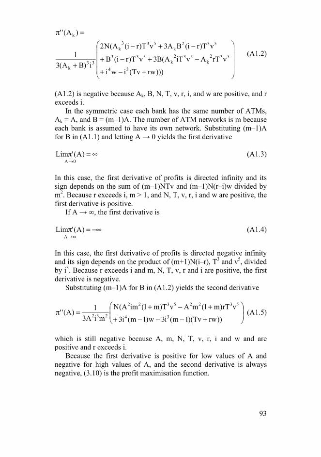
93

⎟⎟⎟⎟

⎠

⎞

⎜⎜⎜⎜

⎝

⎛

+−+

−+−+

−+−

+

=π

)))rwTv(iwi

vrTAviTA(B3vT)ri(B

vT)ri(BA3vT)ri(A(N2

i)BA(31

)A(''

34

532k

532k

533

532k

533k

33k

k

(A1.2)

(A1.2) is negative because Ak, B, N, T, v, r, i, and w are positive, and r exceeds i. In the symmetric case each bank has the same number of ATMs, Ak = A, and B = (m–1)A. The number of ATM networks is m because each bank is assumed to have its own network. Substituting (m–1)A for B in (A1.1) and letting A → 0 yields the first derivative

∞=π→0A

)A('Lim (A1.3)

In this case, the first derivative of profits is directed infinity and its sign depends on the sum of (m–1)NTv and (m–1)N(r–i)w divided by m2. Because r exceeds i, m > 1, and N, T, v, r, i and w are positive, the first derivative is positive. If A → ∞, the first derivative is

−∞=π∞→A

)A('Lim (A1.4)

In this case, the first derivative of profits is directed negative infinity and its sign depends on the product of (m+1)N(i–r), T3 and v5, divided by i3. Because r exceeds i and m, N, T, v, r and i are positive, the first derivative is negative. Substituting (m–1)A for B in (A1.2) yields the second derivative

⎟⎟⎠

⎞⎜⎜⎝

⎛

+−−−+

+−+=π

))rwTv)(1m(i3w)1m(i3

vrT)m1(mAvT)m1(imA(NmiA3

1)A(''34

53225322

232 (A1.5)

which is still negative because A, m, N, T, v, r, i and w and are positive and r exceeds i. Because the first derivative is positive for low values of A and negative for high values of A, and the second derivative is always negative, (3.10) is the profit maximisation function.

94

Appendix 2

ATM network market structure in each country

In this appendix, we describe ATM network market structure in each country, the data of which were used in estimations. These descriptions are based on person-to-person information gathered eg from central banks, other authorities and bankers’ associations, and publications EMI 1996, ECB 2001, and BIS 1985, 1989, 1993 and 2003. Other references are mentioned separately. Austria There is one nationwide ATM network in Austria. In addition, some banks provide ATM services for their own customers only. The data in the ECB statistics include one network in 1990–1995, and the number of networks has not been available since 1996. Typically, cash withdrawals at ATMs are free of charge for consumers. However, there are some limits on monthly transactions. If the number of withdrawals exceeds this limit, the consumer must pay certain fees. Belgium Two interbank ATM networks were introduced in Belgium at the end of the 1970s. These two networks merged in 1989 forming Banksys, which is a common network serving customers of all banks. In addition to this network, several banks offer their own customer in-house terminals, which also provide services other than cash withdrawal. In principle, costs of cash withdrawals have been included in the annual fee. However, banks are starting to charge for withdrawals exceeding a certain amount. Canada The first cash dispenser was installed in Canada in 1969. Nowadays, proprietary networks are typically connected to a shared network, such as Interac, in order to be interoperable with each other. Fees for cash withdrawals vary depending on the owner and location of the ATM.

95

According to BIS statistics, the number of ATM networks in Canada increased from 40 to 77 in 1997–2003. We used these data in the estimations. Denmark There is one ATM network in Denmark. ATM cash withdrawal fees vary depending on the bank and on time of day. Typically, if the consumer withdraws cash at an ATM maintained by another bank or outside business hours, he has to pay a small fee. Finland The first off-line cash withdrawal ATMs were installed in the mid-1970s in Finland (eg Bank of Finland 1993, p. 94). On-line ATMs were introduced in the early 1980s, and some statistics on ATMs have been available since 1984. At first, each bank had its own, incompatible ATM network. Later, these ATM networks were made compatible. In 1994, the biggest banks closed their own networks. They founded a jointly owned company, Automatia Pankkiautomaatit Ltd, which launched a single common ATM network, Otto.network, and began to maintain the ATMs of this network. In addition to Otto.network, there were two small networks, which were closed down in 2004. Since the end of 2004, cash withdrawals at Otto.ATMs have generally been available for consumers of all banks free of charge. Only one small bank charges its customers a fee for withdrawals of less than EUR 80. France ATMs are interoperable in France nowadays, and fees for cash withdrawals vary across banks. There was only one ATM network in 1988–1995, and the data have not been available in ECB or BIS statistics since 1996. Germany Nowadays, banks offer ATM services to both their own and other banks’ customers. According to ECB and BIS statistics, there were

96

four networks during 1988–1998 and one since 1999. However, according to the central bank of Germany, the number of networks has not decreased, but the interpretation of network arrangements has changed. Therefore, we decided to assume the existence of one ATM network for the whole observation period in the estimations. Greece The number of ATM networks fluctuates somewhat from year to year, according to ECB statistics. However, all ATM networks are interoperable, and one must pay a fee for a withdrawal at another bank’s ATM. Ireland ATMs were introduced in Ireland in the early 1980s. According to ECB statistics, the number of ATM networks decreased from three to one in 1996. Bank charges are regulated in Ireland by the Irish Financial Services Regulation Authority. Charges for ATM cash withdrawals vary among banks. Some special groups such as students and pensioners are able to make cash withdrawals without charge. Italy The nationwide ATM network, Bancomat, went into operation in 1983. Nowadays, over 90% of ATMs are interconnected by Bancomat. In ECB and BIS statistics, the number of ATM networks increased from one to four in the 1990s (in 1996 or 1999, depending on the statistics). Because data series have been changed backwards, it seems that there has been a change in the interpretation of the network, not in the actual number of networks. We used four ATM networks since 1996 in the estimations because four ATM service providers manage four ATM/POS sub-networks in Italy. Japan The first cash dispensers were introduced in Japan in 1969 (Japanese Bankers Association 2003, EMEAP 2002). Before 1990, there were many local ATM networks that were not connected with each other. In

97

1990, a system that connects separate networks, MICS, started operations. Since then, many local networks were closed down. Withdrawal fees are often charged for consumers’ use of ATMs of other banks. Since 2000, the number of ATM networks reported in BIS statistics has included only MICS and nine intra-industry networks; local networks have been excluded. Because these data are not consistent with the data published in the earlier years, we used the data for 1988–1999 in the estimations. Luxembourg According to ECB statistics, there were two ATM networks in Luxembourg in 1990–1995 and one since 1996. In addition, some banks have their own, very small networks. Typically, customers do not pay any fees for ATM withdrawals at ATMs maintained by their own bank. However, banks charge customers a fee if they use ATMs of other banks. However, there are exceptions – a few withdrawals per month at other banks' ATMs may be free of charge for the customer. Netherlands The first cash dispensers were installed in 1985 in the Netherlands. The number of ATM networks was reduced from two to one in 1998. Earlier, these two networks were not interoperable. Consumers do not pay for withdrawing cash at other banks’ ATMs. However, there are interchange fees between banks if customers withdraw cash at ATMs of other banks (Bolt 2003). Norway In Norway, ATMs were introduced at the end of the 1970s, and there is one ATM network. Cash withdrawal fees vary across banks (Norges Bank 2004). In most cases, customers are offered free cash withdrawal services at their own banks’ ATMs during business hours. Outside business hours many banks charge a fee. Some banks charge a fee for withdrawals by other banks’ customers also during business hours. (Norges Bank 2004)

98

Portugal In Portugal, there is one nationwide ATM network, which was implemented in 1985. All debit cards are valid in this network and can be used free of charge. In addition to this compatible network, some banks provide to their own customers in-house services. These limited-access terminals are located in bank premises. However, ECB statistics include one network in 1990–1995, and the number of networks has not been available since 1996. We used these data in the estimations. Spain There have been three ATM networks in Spain since the 1970s. All three are fully interoperable. Fees vary between banks and depend eg on the local penetration of the credit institution. Sweden The first ATMs were installed in Sweden in the 1960s. Nowadays, there are two different brands of ATMs, which became interoperable in 1996. These two brands are regarded as one network in BIS and ECB statistics. Customers have always been able to withdraw cash free of charge. Switzerland There are two ATM networks in Switzerland; Bancomat and Postomat. The first Bancomat ATM was installed in 1968. These two ATM networks have been interoperable since 1997. UK The first cash dispensers were introduced in the UK in 1967. At the end of the 1980s, there were four major networks, in 1990–1998 three

99

networks, and since 1999 one network. Nowadays, about a third of ATMs charge a fee for a cash withdrawal (APACS24 2004). USA ATMs were introduced in the USA in the 1960s. The first ATM networks served limited geographical areas and later regional shared ATM networks were established. Still later, national shared networks were introduced (Sienkiewicz 2002). Cash withdrawal fees paid by customers vary widely (eg McAndrews 2003).

24 Association for Payment Clearing Services.

100

Appendix 3

Variable figures

Ln (ATMs per million inhabitants)

5.2

5.4

5.6

5.8

6.0

6.2

6.4

6.6

6.8

84 86 88 90 9 2 94 96 98 00 02

LNA_AU

4 .4

4 .8

5 .2

5 .6

6 .0

6 .4

6 .8

84 8 6 88 90 92 94 96 98 00 02

LNA_BE

5.2

5.6

6.0

6.4

6.8

7.2

7.6

84 86 88 90 92 94 96 98 00 02

LNA_CA

4.5

5.0

5.5

6.0

6.5

84 86 88 90 92 94 96 98 00 0 2

LNA_DE

4.0

4.4

4.8

5.2

5.6

6.0

6.4

84 86 88 90 92 94 9 6 98 00 02

LNA_DK

5.8

6.0

6.2

6.4

6.6

6.8

7.0

7.2

84 86 88 90 9 2 94 96 98 00 02

LNA_ES

5 .9

6 .0

6 .1

6 .2

6 .3

6 .4

84 8 6 88 90 92 94 96 98 00 02

LNA_FI

5.2

5.4

5.6

5.8

6.0

6.2

6.4

6.6

84 86 88 90 92 94 96 98 00 02

LNA_FR

3.0

3.5

4.0

4.5

5.0

5.5

6.0

6.5

84 86 88 90 92 94 96 98 00 0 2

LNA_GR

5.0

5.1

5.2

5.3

5.4

5.5

5.6

5.7

5.8

5.9

84 86 88 90 92 94 9 6 98 00 02

LNA_IE

4.4

4.8

5.2

5.6

6.0

6.4

6.8

84 86 88 90 9 2 94 96 98 00 02

LNA_IT

6 .3

6 .4

6 .5

6 .6

6 .7

6 .8

6 .9

7 .0

84 8 6 88 90 92 94 96 98 00 02

LNA_JP

5.2

5.6

6.0

6.4

6.8

84 86 88 90 92 94 96 98 00 02

LNA_LU

4.0

4.4

4.8

5.2

5.6

6.0

6.4

84 86 88 90 92 94 96 98 00 0 2

LNA_NL

5.96

6.00

6.04

6.08

6.12

6.16

6.20

84 86 88 90 92 94 9 6 98 00 02

LNA_NO

4.0

4.5

5.0

5.5

6.0

6.5

7.0

84 86 88 90 9 2 94 96 98 00 02

LNA_PT

5 .3

5 .4

5 .5

5 .6

5 .7

5 .8

84 8 6 88 90 92 94 96 98 00 02

LNA_SE

5.4

5.6

5.8

6.0

6.2

6.4

6.6

84 86 88 90 92 94 96 98 00 02

LNA_SWI

5.4

5.6

5.8

6.0

6.2

6.4

6.6

6.8

84 86 88 90 92 94 96 98 00 0 2

LNA_UK

5.6

6.0

6.4

6.8

7.2

84 86 88 90 92 94 9 6 98 00 02

LNA_USA

101

Ln (ATM networks)

-1.0

-0.5

0.0

0.5

1.0

84 86 88 9 0 92 94 96 98 0 0 02

LNM_AU

0.8

1.2

1.6

2.0

2.4

2.8

84 8 6 88 90 92 94 9 6 98 00 02

LNM_BE

3.6

3.7

3.8

3.9

4.0

4.1

4.2

4.3

4.4

84 86 88 90 92 94 96 98 00 02

LNM_CA

-1.0

-0.5

0.0

0.5

1.0

84 86 88 90 92 94 96 98 00 02

LNM_DE

-1.0

-0.5

0.0

0.5

1.0

84 86 88 90 92 94 96 98 00 02

LNM_DK

1.04

1.06

1.08

1.10

1.12

1.14

1.16

84 86 88 9 0 92 94 96 98 0 0 02

LNM_ES

0.0

0.2

0.4

0.6

0.8

1.0

1.2

84 8 6 88 90 92 94 9 6 98 00 02

LNM_FI

-1.0

-0.5

0.0

0.5

1.0

84 86 88 90 92 94 96 98 00 02

LNM_FR

1.8

2.0

2.2

2.4

2.6

2.8

3.0

3.2

84 86 88 90 92 94 96 98 00 02

LNM_GR

0.0

0.2

0.4

0.6

0.8

1.0

1.2

84 86 88 90 92 94 96 98 00 02

LNM_IE

1.30

1.32

1.34

1.36

1.38

1.40

1.42

1.44

1.46

84 86 88 9 0 92 94 96 98 0 0 02

LNM_IT

2.4

2.8

3.2

3.6

4.0

4.4

84 8 6 88 90 92 94 9 6 98 00 02

LNM_JP

.0

.1

.2

.3

.4

.5

.6

.7

84 86 88 90 92 94 96 98 00 02

LNM_LU

.0

.1

.2

.3

.4

.5

.6

.7

84 86 88 90 92 94 96 98 00 02

LNM_NL

-1.0

-0.5

0.0

0.5

1.0

84 86 88 90 92 94 96 98 00 02

LNM_NO

-1.0

-0.5

0.0

0.5

1.0

84 86 88 9 0 92 94 96 98 0 0 02

LNM_PT

.0

.1

.2

.3

.4

.5

.6

.7

84 8 6 88 90 92 94 9 6 98 00 02

LNM_SE

.65

.66

.67

.68

.69

.70

.71

.72

.73

84 86 88 90 92 94 96 98 00 02

LNM_SWI

0.0

0.2

0.4

0.6

0.8

1.0

1.2

1.4

84 86 88 90 92 94 96 98 00 02

LNM_UK

3.6

3.8

4.0

4.2

4.4

4.6

4.8

5.0

84 86 88 90 92 94 96 98 00 02

LNM_USA

Ln (cash per capita), real euro prices

6.9

7.0

7.1

7.2

7.3

7.4

84 86 88 9 0 92 94 96 98 0 0 02

LNX_AU

6.4

6.5

6.6

6.7

6.8

6.9

7.0

7.1

7.2

7.3

84 8 6 88 90 92 94 9 6 98 00 02

LNX_BE

6.2

6.3

6.4

6.5

6.6

6.7

84 86 88 90 92 94 96 98 00 02

LNX_CA

6.7

6.8

6.9

7.0

7.1

7.2

7.3

7.4

84 86 88 90 92 94 96 98 00 02

LNX_DE

6.50

6.55

6.60

6.65

6.70

6.75

6.80

84 86 88 90 92 94 96 98 00 02

LNX_DK

6.5

6.6

6.7

6.8

6.9

7.0

7.1

7.2

84 86 88 9 0 92 94 96 98 0 0 02

LNX_ES

5.6

5.7

5.8

5.9

6.0

6.1

6.2

6.3

84 8 6 88 90 92 94 9 6 98 00 02

LNX_FI

6.1

6.2

6.3

6.4

6.5

6.6

6.7

6.8

84 86 88 90 92 94 96 98 00 02

LNX_FR

6.0

6.1

6.2

6.3

6.4

6.5

6.6

84 86 88 90 92 94 96 98 00 02

LNX_GR

6.2

6.3

6.4

6.5

6.6

6.7

6.8

6.9

84 86 88 90 92 94 96 98 00 02

LNX_IE

6.2

6.3

6.4

6.5

6.6

6.7

6.8

6.9

84 86 88 9 0 92 94 96 98 0 0 02

LNX_IT

7.5

7.6

7.7

7.8

7.9

8.0

8.1

8.2

8.3

8.4

84 8 6 88 90 92 94 9 6 98 00 02

LNX_JP

6.6

6.7

6.8

6.9

7.0

7.1

7.2

7.3

84 86 88 90 92 94 96 98 00 02

LNX_LU

6.2

6.4

6.6

6.8

7.0

7.2

7.4

84 86 88 90 92 94 96 98 00 02

LNX_NL

6.70

6.75

6.80

6.85

6.90

6.95

7.00

7.05

84 86 88 90 92 94 96 98 00 02

LNX_NO

5.85

5.90

5.95

6.00

6.05

6.10

6.15

6.20

6.25

84 86 88 9 0 92 94 96 98 0 0 02

LNX_PT

6.76

6.80

6.84

6.88

6.92

6.96

7.00

7.04

84 8 6 88 90 92 94 9 6 98 00 02

LNX_SE

7.84

7.88

7.92

7.96

8.00

8.04

8.08

84 86 88 90 92 94 96 98 00 02

LNX_SWI

6.0

6.1

6.2

6.3

6.4

6.5

6.6

84 86 88 90 92 94 96 98 00 02

LNX_UK

6.7

6.8

6.9

7.0

7.1

7.2

7.3

7.4

84 86 88 90 92 94 96 98 00 02

LNX_USA

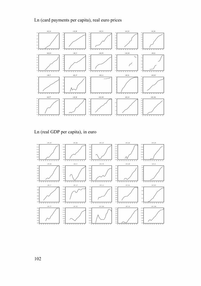
102

Ln (card payments per capita), real euro prices

5.0

5.5

6.0

6.5

7.0

7.5

84 86 88 90 92 94 96 98 00 02

LNZ_AU

5.6

6.0

6.4

6.8

7.2

7.6

8.0

8.4

84 86 88 90 92 94 96 98 00 02

LNZ_BE

7.0

7.2

7.4

7.6

7.8

8.0

8.2

8.4

8.6

8 4 86 88 90 92 94 96 98 00 02

LNZ_CA

5.2

5.6

6.0

6.4

6.8

7.2

7.6

84 86 88 90 92 94 96 98 00 02

LNZ_DE

7.0

7.2

7.4

7.6

7.8

8.0

8.2

8.4

84 8 6 88 90 92 94 96 98 00 02

LNZ_DK

4.8

5.2

5.6

6.0

6.4

6.8

7.2

84 86 88 90 92 94 96 98 00 02

LNZ_ES

6.8

7.0

7.2

7.4

7.6

7.8

8.0

8.2

8.4

84 86 88 90 92 94 96 98 00 02

LNZ_FI

6.6

6.8

7.0

7.2

7.4

7.6

7.8

8.0

8.2

8 4 86 88 90 92 94 96 98 00 02

LNZ_FR

4.4

4.6

4.8

5.0

5.2

5.4

5.6

84 86 88 90 92 94 96 98 00 02

LNZ_GR

5.6

6.0

6.4

6.8

7.2

7.6

84 8 6 88 90 92 94 96 98 00 02

LNZ_IE

3

4

5

6

7

8

84 86 88 90 92 94 96 98 00 02

LNZ_IT

6.4

6.6

6.8

7.0

7.2

7.4

84 86 88 90 92 94 96 98 00 02

LNZ_JP

1

2

3

4

5

6

7

8

9

8 4 86 88 90 92 94 96 98 00 02

LNZ_LU

2

3

4

5

6

7

8

84 86 88 90 92 94 96 98 00 02

LNZ_NL

5.5

6.0

6.5

7.0

7.5

8.0

8.5

9.0

84 8 6 88 90 92 94 96 98 00 02

LNZ_NO

4.5

5.0

5.5

6.0

6.5

7.0

7.5

8.0

84 86 88 90 92 94 96 98 00 02

LNZ_PT

6.0

6.4

6.8

7.2

7.6

8.0

8.4

84 86 88 90 92 94 96 98 00 02

LNZ_SE

5.5

6.0

6.5

7.0

7.5

8.0

8.5

8 4 86 88 90 92 94 96 98 00 02

LNZ_SWI

6.5

7.0

7.5

8.0

8.5

84 86 88 90 92 94 96 98 00 02

LNZ_UK

7.2

7.4

7.6

7.8

8.0

8.2

8.4

8.6

8.8

84 8 6 88 90 92 94 96 98 00 02

LNZ_USA

Ln (real GDP per capita), in euro

9.96

10.00

10.04

10.08

10.12

10.16

10.20

84 86 88 90 92 94 9 6 98 00 02

LNY_AU

9.80

9.85

9.90

9.95

10.00

10.05

10.10

8 4 86 88 90 92 94 96 98 00 02

LNY_BE

9.70

9.75

9.80

9.85

9.90

9.95

10.00

84 86 88 90 92 94 96 98 0 0 02

LNY_CA

1 0.00

1 0.02

1 0.04

1 0.06

1 0.08

1 0.10

1 0.12

1 0.14

84 86 88 9 0 92 94 96 98 00 02

LNY_DE

10.08

10.12

10.16

10.20

10.24

10.28

10.32

84 86 88 90 92 94 96 98 00 02

LNY_DK

9.25

9.30

9.35

9.40

9.45

9.50

9.55

84 86 88 90 92 94 9 6 98 00 02

LNY_ES

9.80

9.85

9.90

9.95

10.00

10.05

10.10

10.15

8 4 86 88 90 92 94 96 98 00 02

LNY_FI

9.84

9.88

9.92

9.96

10.00

10.04

10.08

84 86 88 90 92 94 96 98 0 0 02

LNY_FR

9.00

9.05

9.10

9.15

9.20

9.25

9.30

84 86 88 9 0 92 94 96 98 00 02

LNY_GR

9.3

9.4

9.5

9.6

9.7

9.8

9.9

10.0

10.1

84 86 88 90 92 94 96 98 00 02

LNY _IE

9.45

9.50

9.55

9.60

9.65

9.70

84 86 88 90 92 94 9 6 98 00 02

LNY_ IT

10.08

10.12

10.16

10.20

10.24

10.28

10.32

8 4 86 88 90 92 94 96 98 00 02

LNY _J P

10.2

10.3

10.4

10.5

10.6

10.7

10.8

84 86 88 90 92 94 96 98 0 0 02

LNY _LU

9.75

9.80

9.85

9.90

9.95

1 0.00

1 0.05

1 0.10

84 86 88 9 0 92 94 96 98 00 02

LNY_NL

10.0

10.1

10.2

10.3

10.4

84 86 88 90 92 94 96 98 00 02

LNY_NO

8.90

8.95

9.00

9.05

9.10

9.15

9.20

84 86 88 90 92 94 9 6 98 00 02

LNY_PT

9.90

9.95

10.00

10.05

10.10

10.15

10.20

10.25

8 4 86 88 90 92 94 96 98 00 02

LNY_SE

10.42

10.44

10.46

10.48

10.50

10.52

10.54

84 86 88 90 92 94 96 98 0 0 02

LNY_S WI

9.68

9.72

9.76

9.80

9.84

9.88

9.92

9.96

1 0.00

84 86 88 9 0 92 94 96 98 00 02

LNY_UK

9.85

9.90

9.95

10.00

10.05

10.10

10.15

84 86 88 90 92 94 96 98 00 02

LNY_USA

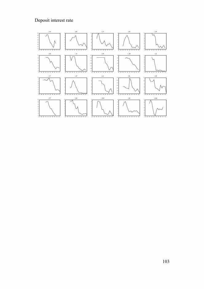
103

Deposit interest rate

1.2

1.6

2.0

2.4

2.8

3.2

3.6

4.0

84 86 88 90 92 94 96 98 00 02

I_AU

1

2

3

4

5

6

7

8

84 86 88 90 92 94 96 98 00 02

I_BE

0

2

4

6

8

10

8 4 86 88 90 92 94 96 98 00 02

I_CA

2

3

4

5

6

7

8

9

84 86 88 90 92 94 96 98 00 02

I_DE

2

3

4

5

6

7

8

84 8 6 88 90 92 94 96 98 00 02

I_DK

0

2

4

6

8

1 0

1 2

84 86 88 90 92 94 96 98 00 02

I_ES

1

2

3

4

5

6

7

8

84 86 88 90 92 94 96 98 00 02

I_FI

2.4

2.8

3.2

3.6

4.0

4.4

4.8

8 4 86 88 90 92 94 96 98 00 02

I_FR

0

4

8

12

16

20

24

84 86 88 90 92 94 96 98 00 02

I_GR

0

1

2

3

4

5

6

7

84 8 6 88 90 92 94 96 98 00 02

I_IE

0

1

2

3

4

5

6

7

8

84 86 88 90 92 94 96 98 00 02

I_IT

0

1

2

3

4

5

84 86 88 90 92 94 96 98 00 02

I_JP

2

3

4

5

6

7

8 4 86 88 90 92 94 96 98 00 02

I_LU

2.4

2.8

3.2

3.6

4.0

4.4

4.8

84 86 88 90 92 94 96 98 00 02

I_NL

2

4

6

8

10

12

84 8 6 88 90 92 94 96 98 00 02

I_NO

2

4

6

8

1 0

1 2

1 4

1 6

84 86 88 90 92 94 96 98 00 02

I_PT

1

2

3

4

5

6

7

8

9

10

84 86 88 90 92 94 96 98 00 02

I_SE

0

1

2

3

4

5

6

7

8

9

8 4 86 88 90 92 94 96 98 00 02

I_SWI

0

2

4

6

8

10

12

14

84 86 88 90 92 94 96 98 00 02

I_UK

3

4

5

6

7

8

9

84 8 6 88 90 92 94 96 98 00 02

I_USA

104

Appendix 4

Unit root tests Pooled unit root tests

In levels

Levin, Lin & Chu Breitung ADF PPATMs per inhabitant; ln(a jt -1) -14,04 2,46 114,12 183,8ATM network; ln(m jt ) -2,71 0,27 16,91 26,96Cash per capita; ln(x jt ) 0,23 2,09 39,25 20,78Card payments per capita; ln(z jt ) -3,49 2,83 34,88 63,06Real GDP per capita; ln(y jt ) -0,64 3,12 10,18 18,42Interest rate; ijt 2,31 -1,84 17,51 11,23

In first differences

Levin, Lin & Chu Breitung ADF PPATMs per inhabitant; ln(a jt -1) -11,65 -1,5 132,49 152,77ATM network; ln(m jt ) -7,1 -5,4 77,08 77,57Cash per capita; ln(x jt ) -1,78 -3,05 79,63 74,74Card payments per capita; ln(z jt ) -7,9 -3,78 109,1 126,65Real GDP per capita; ln(y jt ) -5,63 -4,11 79,51 78,16Interest rate; ijt -10,68 -5,22 120,85 126,37 Bold and italic bold coefficients denote significance at 5% and 1% level, respectively. Levin, Lin and Chu denotes the Levin, Lin and Chu common unit root test, Breitung denotes the Breitung common unit root test, and ADF and PP denote the Augmented Dickey-Fuller and Phillips-Perron individual unit root Fischer tests, respectively.

105

Appendix 5

Symbols and abbreviations

ATM Automated Teller Machine BIS Bank for International Settlements ECB European Central Bank EFTPOS Electronic Funds Transfer Point of Sale SEPA Single Euro Payment Area ajt number of ATMs per million inhabitants in country j in period t mjt number of ATM networks in country j in period t xjt cash in circulation per capita in country j in period t (real euro

prices) zjt value of debit and credit card payments per capita in country j in

period t (real euro prices) djt euro conversion dummy in country j in period t yjt real GDP per capita in country j in period t (in euro) ijt deposit interest rate in country j in period t

Bank of Finland Publications

Scientifi c monographs

Series E (ISSN 1238-1691, print) (ISSN 1456-5951, online)

(Series E replaces the Bank of Finland’s research publications series B, C and D.)

E:1 Jukka Vesala Testing for Competition in Banking: Behavioral Evidence from Finland. 1995. 206 p. ISBN 951-686-447-3.

E:2 Juha Tarkka Approaches to Deposit Pricing: A Study in the Determination of Deposit Interest and Bank Service Charges. 1995. 166 p. ISBN 951-686-457-0.

E:3 Timo Tyrväinen Wage Determination, Ta xes, and Employment: Evidence from Finland. 1995. 212 p. ISBN 951-686-459-7.

E:4 Sinimaaria Ranki Realignment Expectations in the ERM: Causes and Measurement. 1996. 164 p. ISBN 951-686-507-0.

E:5 Juhana Hukkinen Kilpailukyky, ulkomaankaupan rakenne ja taloudellinen kasvu (Competitiveness, structure of foreign trade and economic growth). 1996. 134 p. ISBN 951-686-512-7.

E:6 Eelis Hein Deposit Insurance: Pricing and Incentives. 1996. 120 p. ISBN 951-686-517-8.

E:7 Vesa Vihriälä Banks and the Finnish Credit Cycle 1986–1995. 1997. 200 p. ISBN 951-686-537-2.

E:8 Anne Brunila Fiscal Policy and Private Consumption-Saving Decisions: European Evidence. 1997. 147 p. ISBN 951-686-558-5. (Published also as A-131, Helsinki School of Economics and Business Administration, ISBN 951-791-225-0, ISSN 1237-556X)

E:9 Sinimaaria Ranki Exchange Rates in European Monetary Integration. 1998. 221 p. ISBN 951-686-564-X.

E:10 Kimmo Virolainen Tax Incentives and Corporate Borrowing: Evidence from Finnish Company Panel Data. 1998. 151 p. ISBN 951-686-573-9. (Published also as A-137, Helsinki School of Economics and Business Administration, ISBN 951-791-290-0, ISSN 1237-556X)

E:11 Monica Ahlstedt Analysis of Financial Risks in a GARCH Framework. 1998. 181 p. ISBN 951-686-575-5.

E:12 Olli Castrén Fiscal-Monetary Policy Coordination and Central Bank Independence. 1998. 153 p. ISBN 951-686-580-1.

E:13 Antti Ripatti Demand for Money in Infl ation-Targeting Monetary Policy. 1998. 136 p. ISBN 951-686-581-X.

E:14 Risto Koponen – Kimmo Soramäki Intraday Liquidity Needs in a Modern Interbank Payment System. A Simulation Approach. 1998. 135 p. ISBN 951-686-601-8.

E:15 Liisa Halme Pankkisääntely ja valvonta. Oikeuspoliittinen tutkimus säästöpankkien riskinotosta (Banking regulation and supervision: A legal policy study of risk taking by savings banks). 1999. XLIV + 560 p. ISBN 951-686-606-9, print; ISBN 951-686-607-7, online.

E:16 Juha Kasanen Ilmoitusvelvollisten osakeomistus ja -kaupat Helsingin Pörssissä (Corporate insiders shareholdings and trading on the HEX Helsinki Exchanges). 1999. 146 p. ISBN 951-686-630-1, print; ISBN 951-686-631-X, online.

E:17 Mikko Spolander Measuring Exchange Market Pressure and Central Bank Inter vention. 1999. 118 p. ISBN 951-686-645-X, print; ISBN 951-686-646-8, online.

E:18 Karlo Kauko The Microeconomics of Innovation: Oligopoly Theoretic Analyses with Applications to Banking and Patenting. 2000. 193 p. ISBN 951-686-651-4, print; ISBN 951-686-652-2, online. (Published also as A-166, Helsinki School of Economics and Business Administration, ISBN 951-791-442-3, ISSN 1237-556X)

E:19 Juha Kilponen The Political Economy of Monetary Policy and Wage Bargaining. Theory and Econometric Evidence. 2000. 180 p. ISBN 951-686-665-4, print; ISBN 951-686-666-2, online.

E:20 Jukka Vesala Technological Transformation and Retail Banking Competition: Implications and Measurement. 2000. 211 p. ISBN 951-686-695-6, print; ISBN 951-686-696-4, online. (Published also as A-184, Helsinki School of Economics and Business Administration, ISBN 951-791-518-7, ISSN 1237-556X)

E:21 Jian-Guang Shen Models of Currency Crises with Banking Sector and Imperfectly Competitive Labor Markets. 2001. 159 p. ISBN 951-686-711-1, print; ISBN 951-686-712-X, online.

E:22 Kari Takala Studies in Time Series Analysis of Consumption, Asset Prices and Forecasting. 2001. 300 p. ISBN 951-686-759-6, print; ISBN 951-686-760-X, online.

E:23 Mika Kortelainen Edge: a model of the euro area with applications to monetary policy. 2002. 166 p. ISBN 952-462-001-4, print; ISBN 952-462-002-2, online.(Published also as A-204, Helsinki School of Economics and Business Administration, ISBN 951-791-715-5, ISSN 1237-556X)

E:24 Jukka Topi Effects of moral hazard and monitoring on monetary policy transmission. 2003. 148 p. ISBN 952-462-031-6, print; ISBN 952-462-032-4, online.

E:25 Hanna Freystätter Price setting behavior in an open economy and the determination of Finnish foreign trade prices. 2003. 84 p. ISBN 952-462-045-6, print; ISBN 952-462-046-4, online.

E:26 Tuomas Välimäki Central bank tenders: three essays on money market liquidity auctions. 2003. 232 p. ISBN 952-462-051-0, print; ISBN 952-462-052-9, online.(Published also as A-218, Helsinki School of Economics, Acta Universitatis Oeconomicae Helsingiensis, ISBN 951-791-762-7, ISSN 1237-556X)

E:27 Heikki Hella On robust ESACF identifi cation of mixed ARIMA models. 2003. 159 p. ISBN 952-462-112-6, print; ISBN 952-462-113-4, online.

E:28 Heiko Schmiedel Performance of international securities markets. 2004. 275 p. ISBN 952-462-132-0, print; ISBN 952-462-133-9, online.

E:29 Tuomas Komulainen Essays on fi nancial crises in emerging markets. 2004. 173 p.ISBN 952-462-140-1, print; ISBN 952-462-141-X, online.

E:30 Jukka Vauhkonen Essays on fi nancial contracting. 2004. 134 p. ISBN 952-462-172-X, print; ISBN 952-462-173-8, online.

E:31 Harry Leinonen (ed.) Liquidity, risks and speed in payment and settlement systems – a simulation approach. 2005. Compilation. 350 p. ISBN 952-462-194-0, print; ISBN 952-462-195-9, online.

E:32 Maritta Paloviita The role of expectations in euro area infl ation dynamics. 2005. 88 p.ISBN 952-462-208-4, print; ISBN 952-462-209-2, online.

E:33 Jukka Railavo Essays on macroeconomic effects of fi scal policy rules. 2005. 150 p. ISBN 952-462-249-1, print; ISBN 952-462-250-5, online.

E:34 Aaron Mehrotra Essays on Empirical Macroeconomics. 2006. 243 p.ISBN 952-462-290-4, print; ISBN 952-462-291-2, online.

E:35 Katja Taipalus Bubbles in the Finnish and US equities markets. 2006. 123 p.ISBN 952-462-306-4, print; ISBN 952-462-307-2, online.

E:36 Laura Solanko Essays on Russia’s Economic Transition. 2006. 133 p. ISBN 952-462-316-1, print; ISBN 952-462-317-X, online.

E:37 Mika Arola Foreign capital and Finland Central government’s fi rst period of reliance on international fi nancial markets, 1862–1938. 2006. 249 p. ISBN 952-462-310-2, print; ISBN 952-462-311-0, online.

E:38 Heli Snellman Automated Teller Machine network market structure and cash usage. 2006. 105 p. ISBN 952-462-318-8, print; ISBN 952-462-319-6, online.

ISBN 952-462-318-8ISSN 1238-1691

Edita Prima OyHelsinki 2006

Autom

ated Teller Machine netw

ork market structure and cash usage

Scientific m

onographs E:38 · 2006

automated teller machine network market structure and cash

Documents