author's personal copy - computer science

This article appeared in a journal published by Elsevier. The attachedcopy is furnished to the author for internal non-commercial researchand education use, including for instruction at the authors institution

and sharing with colleagues.

Other uses, including reproduction and distribution, or selling orlicensing copies, or posting to personal, institutional or third party

websites are prohibited.

In most cases authors are permitted to post their version of thearticle (e.g. in Word or Tex form) to their personal website orinstitutional repository. Authors requiring further information

regarding Elsevier’s archiving and manuscript policies areencouraged to visit:

http://www.elsevier.com/authorsrights

http://www.elsevier.com/authorsrights

Author's personal copy

Discrete Optimization 11 (2014) 1–21

Contents lists available at ScienceDirect

Discrete Optimization

journal homepage: www.elsevier.com/locate/disopt

The complexity of probabilistic lobbying✩,✩✩

Daniel Binkele-Raible a, Gábor Erdélyi b, Henning Fernau a,∗, Judy Goldsmith c,Nicholas Mattei d,e,1, Jörg Rothe f

a Universität Trier, Fachbereich 4—Abteilung Informatikwissenschaften, 54286 Trier, Germanyb University of Siegen, School of Economic Disciplines, 57068 Siegen, Germanyc University of Kentucky, Department of Computer Science, Lexington, KY 40506, USAd NICTA, Sydney, Australiae University of New South Wales, Sydney, Australiaf Heinrich-Heine-Universität Düsseldorf, Institut für Informatik, 40225 Düsseldorf, Germany

a r t i c l e i n f o

Article history:Received 22 February 2012Received in revised form 22 October 2013Accepted 26 October 2013Available online 22 November 2013

Keywords:Computational complexityParameterized complexityApproximabilityComputational social choice

a b s t r a c t

We propose models for lobbying in a probabilistic environment, in which an actor (called‘‘The Lobby’’) seeks to influence voters’ preferences of voting for or against multiple issueswhen the voters’ preferences are represented in terms of probabilities. In particular, weprovide twoevaluation criteria and twobriberymethods to formally describe thesemodels,and we consider the resulting forms of lobbying with and without issue weighting. Weprovide a formal analysis for these problems of lobbying, and determine their classicaland parameterized complexity depending on the given bribery/evaluation criteria andon various natural parameterizations. Specifically, we show that some of these problemscan be solved in polynomial time, some are NP-complete but fixed-parameter tractable,and some are W [2]-complete. Finally, we provide approximability and inapproximabilityresults for these problems and several variants.

© 2013 Elsevier B.V. All rights reserved.

1. Introduction

1.1. Motivation and informal description of probabilistic lobbying models

In most democratic political systems, laws are passed by elected officials who are supposed to represent their con-stituency. Individual entities such as citizens or corporations are not supposed to have undue influence in the wordingor passage of a law. However, they are allowed to make contributions to representatives, and it is common to include anindication that the contribution carries an expectation that the representative will vote a certain way on a particular issue.

✩ A preliminary version of this paper appears in the proceedings of the First International Conference on Algorithmic Decision Theory, October 2009 (Erdélyiet al., 2009 [1]).✩✩ This work was done in part while the second author was affiliated to Heinrich-Heine-Universität Düsseldorf and to Nanyang Technological University,Singapore, and visiting Universität Trier, while the first and the fourth author were visiting Heinrich-Heine-Universität Düsseldorf, the sixth author wasvisiting the University of Rochester and Stanford University, and the fifth author was affiliated to the University of Kentucky.∗ Corresponding author. Tel.: +49 6512012827.

E-mail addresses: [email protected] (D. Binkele-Raible), [email protected] (G. Erdélyi), [email protected] (H. Fernau),[email protected] (J. Goldsmith), [email protected] (N. Mattei), [email protected] (J. Rothe).1 NICTA is funded by the Australian Government as represented by the Department of Broadband, Communications and the Digital Economy and the

Australian Research Council through the ICT Centre of Excellence program.

1572-5286/$ – see front matter© 2013 Elsevier B.V. All rights reserved.http://dx.doi.org/10.1016/j.disopt.2013.10.003


2 D. Binkele-Raible et al. / Discrete Optimization 11 (2014) 1–21

Many factors can affect a representative’s vote on a particular issue. There are the representative’s personal beliefs aboutthe issue, which presumably were part of the reason that the constituency elected them. There are also the campaigncontributions, communications from constituents, communications from potential donors, and the representative’s ownexpectations of further contributions and political support.

It is a complicated process to reason about. Earlier work (see the references given in Section 1.2) considered the problemof meting out contributions to representatives in order to pass a set of laws or influence a set of votes. However, the earliercomputational complexity work by Christian et al. [2] on this problemmade the assumption that a politician who accepts acontribution will in fact – if the contribution meets a given threshold – vote according to the wishes of the donor.

It is said that ‘‘An honest politician is one who stays bought’’, but that does not take into account the ongoing pressuresfrom personal convictions and opposing lobbyists and donors. We consider the problem of influencing a set of votes underthe assumption that we can influence only the probability that the politician votes as we desire.

There are several axes along which the picture is being complicated in realistic scenarios. To describe these formally, weintroduce various evaluation criteria and bribery methods. The first one is the notion of sufficiency: What does it mean tosay we have donated enough to influence the vote? Does it mean that the probability that a single vote will go our way isgreater than some threshold? That the probability that all the votes go our way is greater than that threshold? We formallydefine and discuss these and other criteria in the section on evaluation criteria (Section 2.3).

The evaluation criteria we discuss are a proxy for what could be considered the most natural evaluation criteria:probabilistic majority. Ideally, a probabilistic win for an issue would be exactly when the sum of the probabilities of possiblefutures that include that win exceeds a given threshold. This would mean counting all possible future scenarios where awin was achieved. While we do not tackle this question directly in the current work, we study two useful relaxations of thiswinning criteria, which may be easier to express and to analyze algorithmically. In particular, we consider two methods forevaluating the outcome of a vote:

1. strict majority, where a vote on an issue is won by a strict majority of voters having a probability of accepting this issuethat exceeds a given threshold, and

2. average majority, where a vote on an issue is won exactly when the voters’ average probability of accepting this issueexceeds a given threshold.

How does one donate money to a campaign? In the United States there are several laws that influence how, when, andhowmuch a particular person or organization can donate to a particular candidate.We examineways inwhichmoney can bechanneled into the political process in the section on bribery methods (Section 2.2). In particular, we consider twomethodsthat an actor (called ‘‘The Lobby’’) can use to influence the voters’ preferences of voting for or against multiple issues:

1. microbribery, where The Lobby may choose which voter to bribe on which issue in order to influence the outcome of thevote according to the evaluation criterion used and

2. voter bribery, where The Lobby may choose which voters to bribe and for each voter bribed the funds are equallydistributed over all the issues, again aiming at changing the outcome of the vote according to the evaluation criterionused.

The voter bribery method is due to Christian et al. [2], who were the first to study lobbying in the context of directdemocracy where voters vote onmultiple referenda. Their ‘‘Optimal Lobbying’’ problem (denoted OL) is a deterministic andunweighted variant of the lobbying problems that we present in this paper. We state this problem in the standard formatfor parameterized complexity:

Optimal Lobbying

Given: Anm × n 0/1 matrix E and a 0/1 vector Z of length n. Each row ofE represents a voter and each column represents an issue. Anentry of E is 1 if this voter votes ‘‘yes’’ for this issue, and is 0otherwise. Z represents The Lobby’s target outcome.

Parameter: A positive integer b (representing the number of voters to beinfluenced).

Question: Is there a choice of b rows of the matrix (i.e., of b voters) that canbe changed such that in each column of the resulting matrix (i.e.,for each issue) a strict majority vote yields the outcome targetedby The Lobby?

Christian et al. [2] proved that OL is W [2]-complete. Sandholm noted that the ‘‘Optimal Weighted Lobbying’’ (OWL)problem, which allows different voters to have different prices and so generalizesOL, can be expressed as and solved via the‘‘binary multi-unit combinatorial reverse auction winner-determination problem’’ (see [3] for its definition).

The microbribery method in the context of lobbying – though inspired by the different notion of microbribery thatFaliszewski et al. [4,5] introduced in the context of bribery in voting – is new to this paper.


D. Binkele-Raible et al. / Discrete Optimization 11 (2014) 1–21 3

Table 1Complexity results for X-Y-PLP, where X ∈ {MB,VB} and Y ∈ {SM,AM}.

Problem Classical complexity Parameterized complexity, parameterized by Stated in or implied by Thm./Cor.Total budget Budget per issue Total budget & discretiz. level

MB-SM-PLP P (FPT) (FPT) (FPT) 4.1MB-AM-PLP P (FPT) (FPT) (FPT) 4.2VB-SM-PLP NP-complete FPT W [2]-complete FPT 4.3 and 5.1–5.3VB-AM-PLP NP-complete ? W [2]-hard FPT 4.3, 5.4, 5.1

1.2. Related work

Lobbying has been studied formally by economists, computer scientists, and special interest groups since at least 1983 [6]and as an extension to formal game theory since 1944 [7]. The different disciplines have considered mostly disjoint aspectsof the process while seeking to accomplish distinct goals with their respective formal models. Economists study lobbyingas ‘‘economic games’’, as defined by von Neumann and Morgenstern [7]. This analysis is focused on learning how thesecomplex systems work and deducing optimal strategies for winning the competitions [6,8,9]. This work has also focused onhow to ‘‘rig’’ a vote and how to optimally dispense the funds among the various individuals [8]. Economists are interestedin finding effective and efficient bribery schemes [8] as well as determining strategies for instances of two or more players[6,8,9]. Generally, they reduce the problem of finding an effective lobbying strategy to one of finding a winning strategy forthe specific type of game. Economists have also formalized this problem for bribery systems in both the United States [6]and the European Union [10].

The study of lobbying from a computational perspective that was initiated by Christian et al. [2] falls into the field ofcomputational social choice, which stimulates a bidirectional transfer between social choice theory (in particular, voting andpreference aggregation) and computer science. For example, voting systems have been applied in various areas of artificialintelligence, most notably in the design of multiagent systems (see, e.g., [11]), for developing recommender systems [12],for designing a meta-search engine that aggregates the website rankings generated by several search engines [13], etc.Applications of voting systems in such automated settings (not restricted only to political elections in human societies)requires a better understanding of the computational properties of the problems related to voting. In particular,many papershave focused on the complexity of

• winner determination (see, e.g., [14–18]),• manipulation (see, e.g., [5,19–32]),• procedural control (see, e.g., [4,29,33–38]), and• bribery in elections (see, e.g., [4,5]).

Formore details, the reader is referred to the surveys by Faliszewski et al. [39–41], Conitzer [42], and Baumeister et al. [43]and the references cited therein. In comparison, much less work has been done on lobbying in voting on multiple referendathat we are concerned with here ([2], see also [3]).

1.3. Organization of this paper and a brief overview of results

Christian et al. [2] show that OL is complete for the (parameterized) complexity class W [2]. We extend their model oflobbying asmentioned above (see Section 2 for a formal description), and provide algorithms and analysis for these extendedmodels in terms of classical and parameterized complexity. All complexity-theoretic notions needed will be presented inSection 3.

Our classical complexity results (presented in Section 4) are shown via either polynomial-time algorithms for or reduc-tions showing NP-completeness of the problems studied. For the parameterized complexity results (presented in Section 5),we choose natural parameters such as The Lobby’s budget, the budget per referendum, and the ‘‘discretization level’’ usedin formalizing our probabilistic lobbying problems (see Section 2.1). We also consider the concept of issue weighting, mod-eling that certain issues will be of more importance to The Lobby than others. Our classical and parameterized complexityresults are summarized in Table 1 (see Section 4) for problems without and in Table 2 (see Section 4.3) for problems withissue weighting.

In Section 6, we provide approximability and inapproximability results for probabilistic lobbying problems. In this waywe add breadth and depth to not only the models but also the understanding of lobbying behavior. We conclude bysummarizing our main results and stating some open problems in Section 7.

2. Models for probabilistic lobbying

2.1. Initial model

We begin with a version of the Probabilistic Lobbying Problem (PLP, for short) in which voters start with initialprobabilities of voting for an issue and are assigned known costs for increasing their probabilities of voting according to



Table 2Complexity results for X-Y-PLP-WIW, where X ∈ {MB,VB} and Y ∈ {SM,AM}.

Problem Classical complexity Parameterized complexity Stated in or implied by Thm./Cor.Total budget Budget per issue Total budget & discr. level

MB-SM-PLP-WIW NP-complete FPT ? (FPT) 4.4 and 5.6MB-AM-PLP-WIW NP-complete FPT ? (FPT) 4.4 and 5.6VB-SM-PLP-WIW NP-complete FPT W [2]-complete∗ FPT 4.5, 5.7 and 5.8, 5.9VB-AM-PLP-WIW NP-complete ? W [2]-hard FPT 4.5, 5.7 and 5.8

‘‘The Lobby’s’’ agenda by each of a finite set of increments. The question, for this class of problems, is: Given the aboveinformation, along with an agenda and a fixed budget B, can The Lobby target its bribes in order to achieve its agenda?

The complexity of the problem seems to hinge on the evaluation criterion for what it means to ‘‘win a vote’’ or ‘‘achievean agenda’’. We discuss the possible interpretations of evaluation and bribery later in this section.2 First, however, wewill formalize the problem by defining data objects needed to represent the problem instances. (A similar model was firstdiscussed by Reinganum [6] in the continuous case andwe translate it here to the discrete case. This will allow us to presentalgorithms for, and a complexity analysis of, the problem.)

Let Qm×n[0,1] denote the set of m × n matrices over Q[0,1] (the rational numbers in the interval [0, 1]). By slight abuse of

notation,3 we say P ∈ Qm×n[0,1] is a probability matrix (of size m × n), where each entry pi,j of P gives the probability that voter

vi will vote ‘‘yes’’ for referendum (synonymously, for issue) rj. The result of a vote is either a ‘‘yes’’ (represented by 1) or a‘‘no’’ (represented by 0). Thus, we represent the result of any vote on all issues as a 0/1 vector X = (x1, x2, . . . , xn), whichis sometimes also denoted as a string in {0, 1}n.

We now associate with each voter/issue pair (vi, rj) a discrete price function ci,j for changing vi’s probability of voting‘‘yes’’ for issue rj. Intuitively, ci,j is a monotonic staircase function that gives the cost for The Lobby of raising or lowering (indiscrete steps) the ith voter’s probability of voting ‘‘yes’’ on the jth issue. A formal description is as follows.

Given the entries pi,j = ai,j/bi,j of a probabilitymatrix P ∈ Qm×n[0,1] , where ai,j ∈ N = {0, 1, . . .} and bi,j ∈ N>0 = {1, 2, . . .},

choose some k ∈ N such that k + 1 is a common multiple of all bi,j, where 1 ≤ i ≤ m and 1 ≤ j ≤ n, and partition theprobability interval [0, 1] into k + 1 steps of size 1/(k + 1) each.4 The integer k will be called the discretization level of theproblem instance, and each integer κ , 0 ≤ κ ≤ k + 1 might be called a (confidence) step. For each i ∈ {1, 2, . . . ,m} andj ∈ {1, 2, . . . , n}, ci,j : {0, 1/(k+1), 2/(k+1), . . . , k/(k+1), 1} → N is the (discrete) price function for pi,j, i.e., ci,j(ℓ/(k+1))is the price for changing the probability of the ith voter voting ‘‘yes’’ on the jth issue from pi,j to ℓ/(k+1), where 0 ≤ ℓ ≤ k+1.Note that the domain of ci,j consists of k + 2 elements of Q[0,1] including 0, pi,j, and 1. In particular, we require ci,j(pi,j) = 0,i.e., a cost of zero is associated with leaving the initial probability of voter vi voting on issue rj unchanged. Note that k = 0means pi,j ∈ {0, 1}, i.e., in this case each voter either accepts or rejects each issue with certainty and The Lobby can only flipthese results.5 The image of ci,j consists of k + 2 nonnegative integers including 0 (the confidence steps), and we requirethat, for any two elements a, b in the domain of ci,j, if pi,j ≤ a ≤ b or pi,j ≥ a ≥ b, then ci,j(a) ≤ ci,j(b). This guaranteesmonotonicity on the prices in both directions.

We represent the list of price functions associated with a probability matrix P as a table CP , called cost matrix in thefollowing, whose m · n rows give the price functions ci,j and whose k + 2 columns give the costs ci,j(ℓ/(k + 1)), where0 ≤ ℓ ≤ k+ 1. Occasionally, we use ci,j[ℓ] to denote ci,j(ℓ/(k+ 1)), for ℓ ∈ {0, 1, . . . , k+ 1}. Note that we choose the samek for each ci,j, so we have the same number of columns in each row of CP . The entries of CP can be thought of as ‘‘price tags’’indicating what The Lobby must pay in order to change the probabilities of voting.

The Lobby also has an integer-valued budget B and an ‘‘agenda’’, which wewill denote as a vector Z ∈ {0, 1}n for n issues,containing the outcomes The Lobby would like to see on these issues. For The Lobby, the prices for a bribe that moves theoutcomes of a referendum into the wrong direction do not matter. Hence, if Z is zero at position j, then we set ci,j(a) = ––(indicating an unimportant entry) for a > pi,j, and if Z is one at position j, thenwe set ci,j(a) = –– (indicating an unimportantentry) for a < pi,j. Note that ci,j(a) = 0 if and only if a = pi,j.

For simplicity, we may assume that The Lobby’s agenda is all ‘‘yes’’ votes, so the target vector is Z = 1n. This assumptioncan be made without loss of generality, since if there is a zero in Z at position j, we can flip this zero to one and also changethe corresponding probabilities p1,j, p2,j, . . . , pm,j in the jth column of P to 1− p1,j, 1− p2,j, . . . , 1− pm,j (see the evaluation

2 We stress that when we use the term ‘‘bribery’’ in this paper, it is meant in the sense of lobbying [2], not in the sense Faliszewski et al. [5] have in mindwhen defining bribery in elections (see also, e.g., [4,44,45]). In bribery in the context of lobbying one considers modifications to multiple independentissues, while in bribery in the context of elections one generally considers modifying rank orderings of interdependent candidates.3 The term ‘‘probability matrix’’ might be perceived as misleading, since neither the row entries nor the column entries of this matrix must add up to

one. However, we nonetheless use this term to indicate that each matrix entry represents the acceptance probability of a voter for an issue.4 There is some arbitrariness in this choice of k. One might think of more flexible ways of partitioning [0, 1]. We have chosen this way for the sake of

simplifying the representation, but we mention that all that matters is that for each i and j, the discrete price function ci,j is defined on the value pi,j , andis set to zero for this value.5 This is the special case of OL [2].



criteria in Section 2.3 for how to determine the result of voting on a referendum). Moreover, the rows of the cost matrix CPthat correspond to issue j have to be mirrored.

Example 2.1. Consider the following problem instance with k = 9 (so there are k+ 1 = 10 steps),m = 2 voters, and n = 3issues. We will use this as a running example for the rest of this paper. In addition to the above definitions for k, m, and n,we also give the following probability matrix P and cost matrix CP for P . (Note that this example is normalized for an agendaof Z = 13, which is why The Lobby has no incentive for lowering the acceptance probabilities, so those costs are omittedbelow.)

Our example consists of a probability matrix P:

r1 r2 r3v1 0.8 0.3 0.5v2 0.4 0.7 0.4

and the corresponding cost matrix CP :

ci,j 0.0 0.1 0.2 0.3 0.4 0.5 0.6 0.7 0.8 0.9 1.0

c1,1 -- -- -- -- -- -- -- -- 0 100 140c1,2 -- -- -- 0 10 70 100 140 310 520 600c1,3 -- -- -- -- -- 0 15 25 70 90 150c2,1 -- -- -- -- 0 30 40 70 120 200 270c2,2 -- -- -- -- -- -- -- 0 10 40 90c2,3 -- -- -- -- 0 70 90 100 180 300 450

In Section 2.2, we describe two briberymethods, i.e., two specificways inwhich The Lobby can influence the voters. Thesewill be referred to asmicrobribery (MB) and voter bribery (VB). In Section 2.3, we define twoways inwhich The Lobby canwina set of votes. These evaluation criteria will be referred to as strict majority (SM) and average majority (AM). The four basicprobabilistic lobbying problems we will study (each a combination of MB/VB bribery under SM/AM evaluation) are definedin Section 2.4, and a modification of these basic problems with additional issue weighting is introduced in Section 2.5.

2.2. Bribery methods

We begin by first formalizing the bribery methods by which The Lobby can influence votes on issues. We will define twomethods for donating this money.

2.2.1. Microbribery (MB)The first method at the disposal of The Lobby is what we will callmicrobribery.6 We define microbribery to be the editing

of individual elements of the P matrix according to the costs in the CP matrix. Thus The Lobby picks not only which voter toinfluence but also which issue to influence for that voter. This bribery method allows a very flexible version of bribery, andmodels private donations made to politicians or voters in support of specific issues.

More formally, if voter i is bribed with d dollars on issue j, then all entries ci,j[ℓ], 0 ≤ ℓ ≤ k + 1, of CP are updated asfollows:

ci,j[ℓ] :=

–– if (ci,j[ℓ] = ––) ∨ ((ci,j[ℓ] − d) ≤ 0)ci,j[ℓ] − d if (ci,j[ℓ] − d) > 0.

Moreover, assuming The Lobby’s target vector is 1n, let T = argmax{ℓ | ci,j[ℓ] = ––}. Replace ci,j[T ] := 0 and updatepi,j := T/(k + 1).

Example 2.2 (Continuing Example 2.1). To make this concrete, reconsidering our Example 2.1: Suppose we give $100 to thesecond voter and ask her to change her opinion on the third issue. This would lead to the following update of CP :

ci,j 0.0 0.1 0.2 0.3 0.4 0.5 0.6 0.7 0.8 0.9 1.0

c1,1 -- -- -- -- -- -- -- -- 0 100 140c1,2 -- -- -- 0 10 70 100 140 310 520 600c1,3 -- -- -- -- -- 0 15 25 70 90 150c2,1 -- -- -- -- 0 30 40 70 120 200 270c2,2 -- -- -- -- -- -- -- 0 10 40 90c2,3 -- -- -- -- -- -- -- 0 80 200 350

6 Although our notion was inspired by theirs, we stress that it should not be confused with the term ‘‘microbribery’’ used by Faliszewski et al. [4,44,45]in the different context of bribing ‘‘irrational’’ voters in Llull/Copeland elections via flipping single entries in their preference tables.



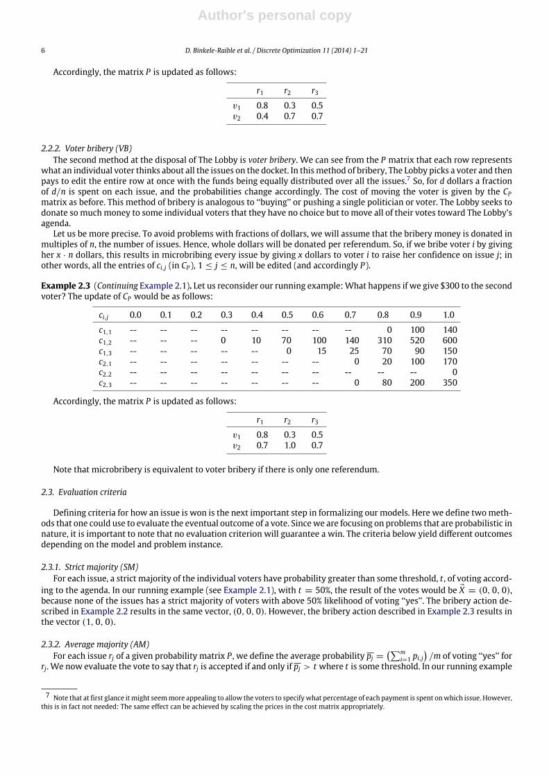
Accordingly, the matrix P is updated as follows:

r1 r2 r3v1 0.8 0.3 0.5v2 0.4 0.7 0.7

2.2.2. Voter bribery (VB)The second method at the disposal of The Lobby is voter bribery. We can see from the P matrix that each row represents

what an individual voter thinks about all the issues on the docket. In thismethod of bribery, The Lobby picks a voter and thenpays to edit the entire row at once with the funds being equally distributed over all the issues.7 So, for d dollars a fractionof d/n is spent on each issue, and the probabilities change accordingly. The cost of moving the voter is given by the CPmatrix as before. This method of bribery is analogous to ‘‘buying’’ or pushing a single politician or voter. The Lobby seeks todonate so muchmoney to some individual voters that they have no choice but to move all of their votes toward The Lobby’sagenda.

Let us be more precise. To avoid problems with fractions of dollars, we will assume that the bribery money is donated inmultiples of n, the number of issues. Hence, whole dollars will be donated per referendum. So, if we bribe voter i by givingher x · n dollars, this results in microbribing every issue by giving x dollars to voter i to raise her confidence on issue j; inother words, all the entries of ci,j (in CP ), 1 ≤ j ≤ n, will be edited (and accordingly P).

Example 2.3 (Continuing Example 2.1). Let us reconsider our running example:What happens if we give $300 to the secondvoter? The update of CP would be as follows:

ci,j 0.0 0.1 0.2 0.3 0.4 0.5 0.6 0.7 0.8 0.9 1.0

c1,1 -- -- -- -- -- -- -- -- 0 100 140c1,2 -- -- -- 0 10 70 100 140 310 520 600c1,3 -- -- -- -- -- 0 15 25 70 90 150c2,1 -- -- -- -- -- -- -- 0 20 100 170c2,2 -- -- -- -- -- -- -- -- -- -- 0c2,3 -- -- -- -- -- -- -- 0 80 200 350

Accordingly, the matrix P is updated as follows:

r1 r2 r3v1 0.8 0.3 0.5v2 0.7 1.0 0.7

Note that microbribery is equivalent to voter bribery if there is only one referendum.

2.3. Evaluation criteria

Defining criteria for how an issue is won is the next important step in formalizing our models. Here we define twometh-ods that one could use to evaluate the eventual outcome of a vote. Sincewe are focusing on problems that are probabilistic innature, it is important to note that no evaluation criterion will guarantee a win. The criteria below yield different outcomesdepending on the model and problem instance.

2.3.1. Strict majority (SM)For each issue, a strict majority of the individual voters have probability greater than some threshold, t , of voting accord-

ing to the agenda. In our running example (see Example 2.1), with t = 50%, the result of the votes would be X = (0, 0, 0),because none of the issues has a strict majority of voters with above 50% likelihood of voting ‘‘yes’’. The bribery action de-scribed in Example 2.2 results in the same vector, (0, 0, 0). However, the bribery action described in Example 2.3 results inthe vector (1, 0, 0).

2.3.2. Average majority (AM)For each issue rj of a given probability matrix P , we define the average probability pj =

mi=1 pi,j

/m of voting ‘‘yes’’ for

rj. We now evaluate the vote to say that rj is accepted if and only if pj > t where t is some threshold. In our running example

7 Note that at first glance itmight seemmore appealing to allow the voters to specifywhat percentage of each payment is spent onwhich issue. However,this is in fact not needed: The same effect can be achieved by scaling the prices in the cost matrix appropriately.



with t = 50%, this would give us a result vector of X = (1, 0, 0). However, the bribery action described in Example 2.2results in the vector (1, 0, 1), while the bribery action described in Example 2.3 results in the vector (1, 1, 1).

Note that the first two criteria coincide if there is only one voter or if the discretization level equals zero.A natural evaluation criteria would be to take into account the probabilities of possible scenarios or futures. Each possible

future, where voters commit to ‘‘yes’’ or ‘‘no’’ votes, has a probability of occurring. If we sum the probabilities of the positivefuture scenarios, we would know the exact probability of a successful outcome. This model has been studied in anotherpaper [46] and led to very complex models. In this paper we have chosen to analyze two proxy models instead, to see ifrelaxing the evaluation criteria leads to easy computational problems.

2.4. Basic probabilistic lobbying problems

We now introduce the four basic problems that we will study. Recalling that, without loss of generality, The Lobby’starget vector may be assumed to be all ones, we define the following problem for X ∈ {MB,VB} and Y ∈ {SM,AM}.

X-Y Probabilistic Lobbying Problem

Given: A probability matrix P ∈ Qm×n[0,1] with a cost matrix CP (with

integer entries), a budget B, and some threshold t ∈ Q[0,1].Question: Is there a way for The Lobby to influence CP and hence P (using

bribery method X and evaluation criterion Y , without exceedingbudget B) such that the result of the votes on all issues equals 1n?

We abbreviate this problem name as X-Y-PLP. Recall that CP has (k + 2)mn many entries.

Example 2.4 (Continuing Example 2.1). Consider voter bribery and the averagemajority criterionwith our running exampleand suppose The Lobby has a budget of $75, i.e., our instance of VB-AM-PLP is (P, CP , 75) with P and CP as given inExample 2.1. Giving $75 to the first voter would suffice to lift all issues above the threshold of 50% on average accordingto the wishes of The Lobby. The updated cost matrix C ′

P would be:

ci,j 0.0 0.1 0.2 0.3 0.4 0.5 0.6 0.7 0.8 0.9 1.0

c1,1 -- -- -- -- -- -- -- -- 0 75 115c1,2 -- -- -- -- 0 45 75 115 285 495 575c1,3 -- -- -- -- -- -- -- 0 45 65 125c2,1 -- -- -- -- 0 30 40 70 120 200 270c2,2 -- -- -- -- -- -- -- 0 10 40 90c2,3 -- -- -- -- 0 70 90 100 180 300 450

This leads to the following updated probability matrix P ′, enriched with the average probabilities:

r1 r2 r3v1 0.8 0.4 0.7v2 0.4 0.7 0.4pj 0.6 0.55 0.55

Since each referendum passes the evaluation test, as desired by The Lobby, (P, CP , 75) is in VB-AM-PLP.

Notice that the discretization level is an implicit (unary) parameter of the problem that is indirectly specified throughthe cost matrix CP .

2.5. Probabilistic lobbying with issue weighting

We now augment the model to include the concept of issue weighting. It is reasonable to surmise that certain issues willbe of more importance to The Lobby than others. For this reason we will allow The Lobby to specify higher weights to theissues that they deem more important. These positive integer weights will be defined for each issue.

Wewill specify theseweights as a vector W ∈ Nn>0 with size n equal to the total number of issues in our problem instance.

The higher the weight, the more important that particular issue is to The Lobby. Along with the weights for each issue weare also given an objective value O ∈ N>0, which is the minimum weight The Lobby wants to see passed. Since this is apartial ordering, it is possible for The Lobby to have an ordering such as w1 = w2 = · · · = wn. If this is the case, we see thatwe are left with an instance of X-Y-PLP, where X ∈ {MB,VB} and Y ∈ {SM,AM}.

We now introduce the four probabilistic lobbying problems with issue weighting. For X ∈ {MB,VB} and Y ∈ {SM,AM},we define the following problem.



X-YProbabilistic Lobbying Problem with Issue Weighting

Given: A probability matrix P ∈ Qm×n[0,1] with cost matrix CP , an issue

weight vector W ∈ Nn>0, an objective value O ∈ N>0, a budget B,

and some threshold t ∈ Q[0,1[.Question: Is there a way for The Lobby to influence CP and hence P (using

bribery method X and evaluation criterion Y , without exceedingbudget B) such that the total weight of all issues for which theresult coincides with The Lobby’s target vector 1n is at least O?

We abbreviate this problem name as X-Y-PLP-WIW.

3. Complexity-theoretic notions

We assume the reader is familiar with standard notions of (classical) complexity theory, such as P , NP, and NP-completeness. Since we analyze the problems stated in Section 2 not only in terms of their classical complexity, but alsowith regard to their parameterized complexity, we provide some basic notions here (see, e.g., the text books by Downey andFellows [47], Flum and Grohe [48], and Niedermeier [49] for more background). As we derive our results in a rather specificfashion, wewill employ the ‘‘Turingway’’ as proposed by Cesati [50]. The reader familiarwith these notions can immediatelyproceed to the next section.

A parameterized problem P is a subset of Σ∗× N, where Σ is a fixed alphabet and Σ∗ is the set of strings over Σ .

Each instance of the parameterized problem P is a pair (I, p), where the second component p is called the parameter. Thelanguage L(P) is the set of all YES instances of P . The parameterized problem P is fixed-parameter tractable if there is analgorithm (realizable by a deterministic Turing machine) that decides whether an input (I, p) is a member of L(P) in timef (p)|I|c , where c is a fixed constant and f is a function of the parameter p, but is independent of the overall input length, |I|.The class of all fixed-parameter tractable problems is denoted by FPT.

Sometimes, more than one parameter (e.g., two parameters (p1, p2)) are associated with a (classical) problem. This isformally captured in the definition above by coding those parameters into one number p via a so-called pairing functionthrough diagonalization. As is standard, we assume our pairing function to be a polynomial-time computable bijection fromN × N onto N that has polynomial-time computable inverses.

For a given classical decision or optimization problem, there are various ways to define parameters. With minimizationproblems, the standard parameterization is a bound on the entity to be minimized. For instance, the problems studied inthis paper have, as a natural minimization objective, the goal to minimize costs (i.e., to use a budget B as small as possible).If one can assume that the parameter p is small in practice, or in practical situations involving humans, we can argue thatan algorithm offering a running time of O(2p

|x|) for an instance x with parameter p behaves reasonably well in practice.Admittedly, this might not be the case with B itself, in particular in view of the fact that only log(B) bits affect the overallsize of the instance. However, this is still the parameter one should start from when considering minimization problems inorder to classify them from the perspective of parameterized complexity.

Are there (more) reasonable, i.e., smaller parameters worth investigating? A related natural parameter choice would bethe budget that can be spent per issue, i.e., the entity B/n. If the voters are actual human beings, one can also argue that thediscretization level k would not be too large.

One of the current trends in parameterized complexity analysis is to studymultiple parameterizations for each problem,including combining multiple parameters for a problem instance. This trend is highlighted by two recent invited talks givenby Fellows [51] and Niedermeier [52]. Notice that the study of different and multiple parameterizations can also be seenfrom another angle: Apart from identifying the hard parts of the problem instance, such research represents a naturalmathematical counterpart of themore practically oriented quest for good parameters thatmay lead to themost competitivealgorithm frameworks for hard problems, as exemplified most notably by SATzilla and ParamILS in the areas of algorithmsfor Satisfiability and Integer Linear Programming, respectively, see [53,54].

There is also a theory of parameterized complexity, as exhibited in [47–49],where parameterized complexity is expressedvia hardness for or completeness in the levelsW [t], t ≥ 1, of theW -hierarchy, which includes fixed-parameter tractabilityat its lower end and is built on top of it to characterize, level by level, higher degrees of parameterized intractability:

FPT = W [0] ⊆ W [1] ⊆ W [2] ⊆ · · · .

It is commonly believed that this hierarchy is strict. Since only the second level,W [2], will be of interest to us in this paper,we will define only this class below.

Definition 3.1. Let P and P ′ be two parameterized problems. A parameterized reduction from P to P ′ is a function r that,for some polynomial q and some function g , is computable in time O(g(p)q(|I|)) and maps an instance (I, p) of P to aninstance r(I, p) = (I ′, p′) of P ′ such that

1. (I, p) is a YES instance of P if and only if (I ′, p′) is a YES instance of P ′, and2. p′

≤ g(p).



We then say that P parameterized reduces to P ′ (via r). Parameterized hardness for and completeness in a parameterizedcomplexity class is defined via parameterized reductions. We will show only W [2]-completeness results. A parameterizedproblem P ′ is said to be W [2]-hard if every parameterized problem P in W [2] parameterized reduces to P ′. P ′ is said tobeW [2]-complete if P ′ is inW [2] and isW [2]-hard.

Notice that one can find at least two other competing definitions of parameterized reduction in the literature: the secondcondition, p′

≤ g(p), is sometimes restricted to p′≤ p and sometimes only requires p′

≤ f (p) for some function f that neednot coincide with the function g occurring in the running time bound. In particular, the second variant is easily seen to beequivalent to our formulation, as g ′(x) = max{g(x), f (x)} shows that a reduction being computable in time O(g(p)q(|I|))and also satisfying p′

≤ f (p) is clearly computable in time O(g ′(p)q(|I|)) and verifies p′≤ g ′(p).

W [2] can be characterized by the following problem on Turing machines:

Short Multi-tape Nondeterministic Turing Machine Computation

Given: A multi-tape nondeterministic Turing machineM (with two-way infinite tapes) andan input string x (bothM and x are given in some standard encoding).

Parameter: A positive integer k.Question: Is there an accepting computation of M on input x that reaches a final accepting

state in at most k steps?

Note that the complexity of Short Multi-tape Nondeterministic Turing Machine Computation crucially depends onthe choice of parameters [47]. It is also important that the machine accesses its tapes in parallel.

More specifically, a parameterized problem P is inW [2] if and only if it can be reduced to Short Multi-tape Nondeter-ministic TuringMachine Computation via a parameterized reduction [50]. This can be accomplished by giving an appropri-ate multi-tape nondeterministic Turing machine for solving P . Hardness forW [2] can be shown by giving a parameterizedreduction in the opposite direction, from Short Multi-tape Nondeterministic Turing Machine Computation to P .

For other applications of fixed-parameter tractability and parameterized complexity to problems from computationalsocial choice, see, e.g., [55].

4. Classical complexity results

We now provide a formal complexity analysis of the probabilistic lobbying problems for all combinations of briberymethods X ∈ {MB,VB} and evaluation criteria Y ∈ {SM,AM}. Table 1 summarizes some of our (classical and parameterized)complexity results for the problems X-Y-PLP; note that Table 1 does not cover Theorem 5.5 (which considers a combinationof two parameters, namely of budget per issue and discretization level).

Some of these results are known from previous work by Christian et al. [2], as will be mentioned below. Our resultsgeneralize theirs by extending the model to probabilistic settings. The listed FPT results might look peculiar at first glance,since Christian et al. [2] derivedW [2]-hardness results, but this is due to the chosen parameterization, as will be discussedlater in more detail. We put parentheses around some classes in Table 1 to indicate that these results are trivially inheritedfrom others. For example, if some problem is solvable in polynomial time, then it is in FPT for any parameterization. Thetable mainly provides results on the containment of problems in certain complexity classes; if known, additional hardnessresults are also listed.

In Section 4.1 we present our results on microbribery (i.e., we study the problems MB-Y-PLP for Y ∈ {SM,AM}), and inSection 4.2 we are concerned with voter bribery (i.e., we study the problems VB-Y-PLP for Y ∈ {SM,AM}). In addition, inSection 4.3 we study probabilistic lobbying with issue weighting.

4.1. Microbribery

Theorem 4.1. MB-SM-PLP is in P.

Proof. The aim is to win all referenda. For each voter vi and referendum rj, 1 ≤ i ≤ m and 1 ≤ j ≤ n, we compute inpolynomial time the amount b(vi, rj) The Lobby has to spend to turn the favor of vi in the direction of The Lobby (beyondthe given threshold t). In particular, set b(vi, rj) = 0 if voter vi would already vote according to the agenda of The Lobby. Foreach issue rj, sort {b(vi, rj) | 1 ≤ i ≤ m} nondecreasingly, yielding a sequence b1(rj), . . . , bm(rj) such that bk(rj) ≤ bℓ(rj) fork < ℓ. To win referendum rj, The Lobby must spend at least B(rj) =

⌈(m+1)/2⌉i=1 bi(rj) dollars. Hence, all referenda are won if

and only ifn

j=1 B(rj) is at most the given bribery budget B. �

Note that the time needed to implement the algorithm given in the previous proof can be bounded by a polynomial oflow order. More precisely, if the input consists of m voters, n referenda, and discretization level k, then O(n · m · k) time isneeded to compute the b(vi, rj). Having these values, O(n · m · logm) time is needed for the sorting phase. The sums can becomputed in timeO(n ·m). (Note that the time analysis can still be improved; however, a rough estimate of the computationtime needed is enough to establish Theorem 4.1.)



Similarly, the other problems that we show to belong to P admit solution algorithms bounded by polynomials of loworder.

Theorem 4.2. MB-AM-PLP is in P.

Proof. Let (P, CP , B, t) be a given MB-AM-PLP instance, where P ∈ Qm×n[0,1] , CP is a cost matrix, B is The Lobby’s budget, and t

is a given threshold. Let k be the discretization level of P , i.e., the interval is divided into k + 1 steps of size 1/(k + 1) each.For j ∈ {1, 2, . . . , n}, let dj be theminimum cost for The Lobby to bring referendum rj into line with the jth entry of its targetvector 1n. If

nj=1 dj ≤ B, then The Lobby can achieve its goal that the votes on all issues pass.

We show that for a fixed j we can compute dj in polynomial time. Therefore, the decision problem of whether TheLobby can afford to bring all referenda into line with its target vector is also in P . We compute dj by dynamic program-ming. The aim is to have

mi=1 pi,j/m > t , i.e.,

mi=1 pi,j > mt . Recall that pi,j · (k + 1) always gives an integer. Define

cj = (k+1)(mt−m

i=1 pi,j)+1. This is the overall number of confidence steps The Lobbyhas to buy towin referendum rj. Notethat cj is polynomial in the size of the input, as ismtk. We define T [l, s] to be the minimum cost of raising (k+ 1)(

mi=1 pi,j)

by value s ≤ cj using only microbribes to the first l voters. Notice that T [l, 0] = 0. Let qi,j be the integer with ci,j[qi,j] = 0.Hence, for κ with 0 ≤ κ < qi,j, we find ci,j[κ] = ––, and for κ with qi,j < κ ≤ k + 1, we have ci,j[κ] > 0. This means thatqi,j/(k + 1) = pi,j. As the maximum number of confidence steps we can gain by bribing voter i is k + 1 − qi,j, we obtain

T [1, s] =

∞ if s > k + 1 − q1,j,c1,j[q1,j + s] otherwise.

Based on this initialization, we can compute:

T [l, s] = minT [l − 1, s − q] + cl,j[ql,j + q] | 0 ≤ q ≤ min{s, k + 1 − ql,j}

.

In particular, q = 0 covers the case when no money is spent on voter l, as cl,j[ql,j] = 0. Thus, each of the polynomially manyentries, T [l, s], can be computed in polynomial time. In particular, T [m, cj] = dj can be computed in polynomial time. �

4.2. Voter bribery

Recall the Optimal Lobbying problem (OL) defined in Section 1.1. Again, The Lobby’s target vector Z may be assumed tobe all ones, without loss of generality, so Z may be dropped from the input.

Christian et al. [2] proved that this problem is W [2]-complete by reducing from the W [2]-complete problem k-Dominating Set to OL (showing the lower bound) and from OL to theW [2]-complete problem Independent-k-DominatingSet (showing the upper bound). In particular, this implies NP-hardness of OL.

The following result focuses on the classical complexity of VB-SM-PLP and VB-AM-PLP; the parameterized complexity ofthese problems will be studied in Section 5 and will make use of the proof of Theorem 4.3 below.

To employ the W [2]-hardness result of Christian et al. [2], we show that OL is a special case of VB-SM-PLP and thus(parameterized) polynomial-time reduces to VB-SM-PLP. Analogous arguments apply to VB-AM-PLP.

Theorem 4.3. VB-SM-PLP and VB-AM-PLP are NP-complete.

Proof. Membership in NP is obtained through a ‘‘guess-and-check’’ algorithm for VB-SM-PLP and VB-AM-PLP.We now prove that VB-SM-PLP is NP-hard by reducing OL to VB-SM-PLP. We are given an instance (E, b) of OL, where E

is am × n 0/1 matrix and b is the number of votes to be edited. Recall that The Lobby’s target vector is 1n. We construct aninstance of VB-SM-PLP consisting of the given matrix P = E (a ‘‘degenerate’’ probability matrix with only the probabilities0 and 1), a corresponding cost matrix CP , and a budget B. CP has two columns (we have k = 0, since the problem instanceis deterministic, see Section 2.1), one column for probability 0 and one for probability 1. All entries of CP corresponding topi,j = 1 are set to unit cost: ci,j[1] = 1 if pi,j = 1. The threshold t is set to 1/2.

The cost of increasing any value in P is n, since donations are distributed evenly across issues for a given voter. We wantto knowwhether there is a set of bribes of cost at most b · n = B such that The Lobby’s agenda passes. This holds if and onlyif there are b voters that can be bribed so that they vote uniformly according to The Lobby’s agenda and that is sufficient topass all the issues. Thus, the given instance (E, b) is inOL if and only if the constructed instance (P, CP , B, t) is in VB-SM-PLP,which shows that OL is a polynomial-time recognizable special case of VB-SM-PLP, and thus VB-SM-PLP is NP-hard.

Note that for the construction above it does not matter whether we use the strict-majority criterion (SM) or the average-majority criterion (AM). Since the entries of P are 0 or 1, we have pj > 0.5 if and only if we have a strict majority of ones inthe jth column. Thus, VB-AM-PLP is NP-hard, too. �


Table 2 summarizes some of our results for X-Y-PLP-WIW, where X ∈ {MB,VB} and Y ∈ {SM,AM}; again, note thatTable 2 does not cover all our results. The most interesting observation from the table is that introducing issue weights



raises the complexity from P to NP-completeness for all cases ofmicrobribery (though it remains the same for voter bribery).Nonetheless, we show (Theorem 5.6) that these NP-complete problems are fixed-parameter tractable. Another interestingobservation concerns the question of membership in W [2]. In the case indicated by the ∗ annotation, we can show thismembership only when we take the lower bound O quantifying the objective of the bribery (in terms of issue weights) as afurther parameter. Question marks indicate open problems.

Theorem 4.4. MB-SM-PLP-WIW and MB-AM-PLP-WIW are each NP-complete.

Proof. Membership in NP can be shown with a ‘‘guess-and-check’’ algorithm for both problems. To prove thatMB-SM-PLP-WIW is NP-hard, we give a reduction from the well-known NP-complete problem Knapsack (see, e.g., [56])to the problem MB-SM-PLP-WIW. In Knapsack, we are given a set of objects U = {o1, . . . , on} with weights w : U → Nand profits p : U → N, and W , P ∈ N. The question is whether there is a subset J ⊆ {1, . . . , n} such that

i∈J w(oi) ≤ W

and

i∈J p(oi) ≥ P . Given a Knapsack instance (U, w, p,W , P), create an MB-SM-PLP-WIW instance with k = 0 and onlyone voter, v1, where for each issue, v1’s acceptance probability is either zero or one. For each object oj ∈ U , create an issuerj such that the acceptance probability of v1 is zero. Let the cost of raising this probability on rj be c1,j(1) = w(oj) and let theweight of issue rj be wj = p(oj). Let The Lobby’s budget be W and its objective value be O = P . Set the threshold t to 1/2.By construction, there is a subset J ⊆ {1, . . . , n} with

i∈J w(oi) ≤ W and

i∈J p(oi) ≥ P if and only if there is a subset

J ⊆ {1, . . . , n} with

i∈J c1,i(1) ≤ W and

i∈J wi ≥ O.As the reduction introduces only one voter, there is no difference between the evaluation criteria SM and AM. Hence, the

above reduction works for both problems. �

Turning now to voter bribery with issue weighting, note that an immediate consequence of Theorem 4.3 is thatVB-SM-PLP-WIW and VB-AM-PLP-WIW are NP-hard, since they are generalizations of VB-SM-PLP and VB-AM-PLP, respec-tively. Again,membership inNP can be seen using appropriate ‘‘guess-and-check’’ algorithms for themore general problems.

Corollary 4.5. VB-SM-PLP-WIW and VB-AM-PLP-WIW each are NP-complete.

NP-completeness of our problems with issue weighting implies that bribery/lobbying is hard in these settings, at leastin the classical sense of worst-case complexity. However, in Section 5 we will provide some positive worst-case results forthese problems in terms of their fixed-parameter tractability, and in Section 6 we will show that many of these problemsadmit good approximation schemes and may therefore be easy to solve in practice.

5. Parameterized complexity results

In this section, we study the parameterized complexity of our probabilistic lobbying problems. Parameterized hardnessis usually shown by proving hardness for the levels of theW -hierarchy (with respect to parameterized reductions). Indeed,this hierarchy may be viewed as a ‘‘barometer of parametric intractability’’ [47, p. 14]. The lowest two levels of theW -hierarchy, W [0] = FPT and W [1], are the parameterized analogs of the classical complexity classes P and NP. We willshow completeness results for theW [2] level of this hierarchy.

In parameterized complexity, the standard parameterization for minimization problems is an upper bound on the entityto be minimized. In our case, this is the budget B. Since in the voter bribery model, the money is equally distributed overall referenda, it also makes sense to consider the upper bound B/n, i.e., the budget per referendum, as a natural, derivedparameter for that scenario. A different, moremathematical reason for considering this parameter is the fact that, first of all,with the parameter B alone, most problems will find their home in the lowest complexity class, FPT, so it is reasonable toconsider parameters that are distinctively smaller than B, which clearly applies to B/n. In particular, while Bmight be quite abig number, B/n can be assumed to be small in practical circumstances. Another natural way of parameterization is derivedfrom certain properties of the input, be they implicit or explicit. In our case, the discretization level can be considered assuch a parameter, in particular, since the smallest discretization level has been already considered beforewithin the optimallobbyingproblem [2]. Therefore,we examine all three of these parameterizations in order to understand the effect the choiceof parameterizations has on the complexity of the problems.

5.1. Voter bribery

Theorem 5.1. VB-SM-PLP and VB-AM-PLP parameterized by the budget and by the discretization level are in FPT.

Proof. Consider an instance of VB-Y-PLP, Y ∈ {SM,AM}, i.e., we are given n referenda andm voters, as well as a cost matrixCP (with either –– or integer entries), a discretization level k, a budget B, and a threshold t . Recall that the target vectorZ of The Lobby is assumed to be 1n. By the definition of our staircase price functions, the rows of CP are monotonicallynondecreasing (after possibly some –– entries). Observe that any successful bribe of any voter needs at least n dollars, sincethe money is evenly distributed among all referenda, and at least one dollar is needed to influence the chosen voter’s votesfor all referenda. Hence, B ≥ n. We can assume that any entry in CP is limited by B + 1, after replacing every entry biggerthan B by B + 1. Notice that the entry B + 1 reflects that the intended bribery cannot be afforded.



Although k could be bigger than B, the interesting area of each row in CP (containing integer entries) cannot have morethan B strict increases in the sequence. We therefore encode each row in CP by a sequence (k1, b1, k2, b2, . . . , kℓ, bℓ), ℓ ≤ B,which reads as follows: By investing bj dollars, we proceed to column number

i≤j ki. Note that k is given in unary in the

original instance (implicitly by giving the cost matrix CP ), and that each kj can be encoded with log k bits. Hence, we extractfromCP for each voter v a submatrix SP(v)withn ≤ B rows (for the referenda) and atmost 2B columns (encoding the ‘‘jumps’’in the integer sequence as described above). This matrix with at most B rows and at most 2B columns can be alternativelyviewed as a matrix with at most B rows and at most B columns, where each matrix entry consists of a pair of numbers, onebetween 1 and B + 1 and one being at most k. Therefore, we can associate with each voter at most ((B + 1) · k)B

2distinct

submatrices SP(v) of this kind, called voter profiles. It makes no sense to store more than B voters with the same profile.Hence, we can assume that m ≤ B · ((B + 1) · k)B

2. Therefore, all relevant parts of the input are bounded by a function in

the parameters B and k,8 so that a brute-force algorithm can be used to solve the instance. This shows that the problem isin FPT. �

If we assume that the discretization level is a rather small number, the preceding theorem says that the problemsVB-SM-PLP and VB-AM-PLP can be solved efficiently in practice. Although we were not able to establish an FPT result forVB-AM-PLPwhen the discretization level is not part of the parameter (but only the budget is), we can overcome this formalobstacle for VB-SM-PLP, as the following result shows.

Theorem 5.2. VB-SM-PLP parameterized by the budget is in FPT.

Proof. Let an instance of VB-SM-PLP be given. From the given cost matrix CP , we extract the information W (i, j) that givesthe minimum amount of money The Lobby must spend on voter vi to turn his or her voting behavior on issue rj in favorof The Lobby’s agenda, eventually raising the corresponding voting probability beyond the given threshold t . Each entry inW (i, j) is between 0 and B. Moreover, as argued in the previous proof, there are no more than B issues and we again definea voter profile (this time the ith row of the table W (i, j) gives such a profile) for each voter, and we need to keep at most Bvoters with the same profile. Hence, no more than B(B+ 1)B voters are present in the instance. Therefore, some brute-forceapproach can be used to show membership in FPT. �

The area of parameterized complexity leaves some freedom regarding the choice of parameterization. The main reasonthat the standard parameterization (referring to the entity to be minimized, in this case the budget) yields an FPT resultis the fact that the parameter is already very big compared to the overall input (e.g., the number of issues n) by the verydefinition of the problem: Since the money given to one voter will be evenly distributed among the issues and since thecost matrix contains only integer entries, it makes no sense at all to spend less than n dollars on a voter. Hence, the budgetshould be at least n dollars (assuming that some of the votersmust be influenced by The Lobby to achieve their agenda). Thisobstacle can be sidestepped by changing the parameterization to B/n, i.e., to the ‘‘budget per issue’’ (see, e.g., Theorem 5.3).Note that another way would be allowing rational numbers as entries in the cost matrix but we will not consider this in thispaper but rather focus on the ‘‘budget per issue’’.

Theorem 5.3. VB-SM-PLP parameterized by the budget per issue is W [2]-complete.

Proof. W [2]-hardness can be derived from the proof of Theorem 4.3. Recall that in the proof of this theorem an instance(E, b) of OL was reduced to an instance of VB-SM-PLP, with budget B = n · b. Hence, the parameter ‘‘budget per issue’’ ofthat VB-SM-PLP instance equals b. Therefore, the reduction in the proof of Theorem 4.3 preserves the parameter and henceW [2]-hardness follows from the W [2]-hardness of OL, see [2]. Moreover, the instance of VB-SM-PLP produced by thereduction has discretization level zero.

To show membership in W [2], we reduce VB-SM-PLP to Short Multi-tape Nondeterministic Turing MachineComputation, which was defined in Section 3. To this end, it suffices to describe how a nondeterministic multi-tape Turingmachine can solve such a lobbying problem.

Consider an instance ofVB-SM-PLP: a probabilitymatrix P ∈ Qm×n[0,1] with a costmatrix CP , a budget B, and a fixed threshold

t . We may identify t with a certain step level for the price functions.The reducing machine works as follows. From P , CP , and t , the machine extracts the information Hi,j(d), 1 ≤ d ≤ B,

where Hi,j(d) is true if pi,j ≥ t or if ci,j(t) ≤ d/n. Note that the bribery money is evenly distributed across all issues, alsonote that Hi,j(d) captures whether paying d dollars to voter vi helps to raise the acceptance probability of vi on referendumrj above the threshold t . Moreover, for each referendum rj, the reducing machine computes the minimum number of votersthat need to switch their opinion so that majority is reached for that specific referendum; let s(j) denote this threshold forrj. Since the cost matrix contains integer entries, meaningfully bribing s voters costs at least s · n dollars; only then eachreferendum will receive at least one dollar per voter. Hence, a referendum with s(j) > B/n yields a NO instance. We cantherefore replace any value s(j) > B/n by the value ⌊B/n⌋ + 1.

FromHi,j(d), the reducingmachine produces (basically by sorting) anotherwinning tableWi(ℓ) that lists for voter vi thosereferenda where the acceptance probability of vi on referendum rj is raised above the threshold t by paying to vi the amount

8 In technical terms, this means that we have derived a so-called problem kernel for this problem.



of ℓ · n dollars but not by paying (ℓ − 1) · n dollars. Note that we can assume that the bribery money is spent in multiplesof n, the number of referenda, since spending n dollars on some voter means spending one dollar per issue for that voter.This table is initialized byWi(0) listing those referenda already won at the very beginning, although this is not an importantissue due to the information contained in s(j).

The nondeterministic multi-tape TuringmachineM we describe next has, in particular, access toWi(ℓ) and to s(j).M hasn + 1 working tapes Tj, 0 ≤ j ≤ n, all except one of which correspond to issues rj, 1 ≤ j ≤ n. We will use the set of voters,V = {v1, . . . , vm}, as part of the work alphabet. The (formal) input tape ofM is ignored.

M starts by writing s(j) symbols # onto tape j for each j, 1 ≤ j ≤ n. By using simultaneous writing steps, this needs atmost ⌊B/n⌋ + 1 steps, since s(j) ≤ ⌊B/n⌋ + 1 as argued above. We also need an ‘‘information hiding’’ trick here: Every timethe machine writes a # symbol, it simultaneously moves the writing head one field to the right, so that in the next step thehead will read a blank symbol. The trick is required in order to keep the transition table small: basically, we cannot insert inthe transition table 2n different instructions to take into account all different configurations of blank and # symbols on then tapes.

Second, for each i ∈ {1, . . . ,m}, M writes ki symbols vi from the alphabet V on the zeroth tape, T0, such thatm

i=1 ki ≤

B/n. This is the nondeterministic guessing phase where the amount of bribery money spent on each voter, namely ki · n forvoter vi, is determined. The finite control is used to ensure that a word from the language {v1}

∗· {v2}

∗· · · {vm}

∗ is writtenon tape T0.

In the third phase, M reads tape T0. In its finite control, M stores the ‘‘current voter’’ whose bribery money is read. Foreach voter vi, a counter ci is provided (within the finite memory of M). If a symbol vi is read, ci is incremented, and then Msimultaneouslymoves all heads on the tapes Tj, where j is contained inWi(ci). Hence, the string on tape T0 is being processedin at most B/n (simultaneous) steps.

Finally, it is checked if the left border is reached (again) for all tapes Tj, j > 0. This is the case if and only if the guessedbribery was successful. �

TheW [2]-hardness proof for VB-AM-PLP is analogous.Recall that VB-SM-PLP is the same as VB-AM-PLP if the discretization level is zero. So, we conclude:

Corollary 5.4. VB-AM-PLP parameterized by the budget per issue is W [2]-hard.

Membership in W [2] is an open problem for VB-AM-PLP when parameterized by the budget per issue. In contrast, weshow definitive parameterized complexity results for different parameterizations. Refining and re-analyzing the proof ofTheorem 5.3, we can prove:

Theorem 5.5. VB-SM-PLP and VB-AM-PLP parameterized by the budget per issue and by the discretization level areW [2]-complete.


Recall fromTheorem4.4 thatMB-SM-PLP-WIW andMB-AM-PLP-WIW areNP-complete.We now show that each of theseproblems is fixed-parameter tractablewhen parameterized by the budget. To this end, recall theKnapsack problem thatwasdefined in the proof of Theorem 4.4: Given two finite lists of binary encoded integers, (ci)ni=1 (a list of costs) and (pi)ni=1 (a listof profits) associated to a list (oi)ni=1 of objects, as well as two further integers, C and P (both encoded in binary), the questionis whether there is a subset J of {1, . . . , n} such that

i∈J ci ≤ C and

i∈J pi ≥ P . Thus, putting all objects from {oj | j ∈ J}

into your knapsack does not violate your cost constraint C but does satisfy your profit demand P . Knapsack is an NP-hardproblem that allows a pseudo-polynomial time algorithm. More precisely, this means that if all cost or all profit values aregiven in unary, a polynomial-time algorithm can be provided by using dynamic programming (see [57] for details). Thisyields FPTAS results both for the minimization version Min-Knapsack (where the goal is to minimize the costs, subject tothe profit lower bound) and for themaximization versionMax-Knapsack (where the goal is to maximize the profits, subjectto the cost upper bound).

Theorem 5.6. MB-SM-PLP-WIW and MB-AM-PLP-WIW parameterized by the budget or by the objective are in FPT.

Proof. Since the unweighted variants of both problems are in P , we can compute the amount dj of dollars to be spent to winreferendum rj in polynomial time in both cases. Namely, dj is the smallest budget that is necessary to win in the instancethat is derived from the given one by deleting everything that is independent of referendum rj. Hence, the interesting casesare the weighted ones. We re-interpret the givenMB-Y-PLP-WIW instance, where Y ∈ {SM,AM}, as a Knapsack instance.

In the MB-Y-PLP-WIW instance, every issue rj has an associated cost dj and weight wj. The aim is to find a set of issues,i.e., a set J ⊆ {1, . . . , n}, such that

j∈J dj ≤ B and

j∈J wj ≥ O. Consider rj as an object oj in a Knapsack instance

with cost cj = dj and profit pj = wj, with the bounds C = B and P = O. Then the J ⊆ {1, . . . , n} that is a solutionto the MB-Y-PLP-WIW instance is also a solution to the Knapsack instance, and vice-versa. Furthermore, the pseudo-polynomial algorithm that solves Knapsack in time O(n2|B|), where |B| denotes the length of the encoding of B, also solvesMB-Y-PLP-WIW. Alternatively,we canuse thewell-knownpseudo-polynomial algorithm to solveKnapsack in timeO(n2|O|),where |O| denotes the length of the encoding of O. �



Voter bribery with issue weighting keeps its complexity status for both evaluation criteria.Since we can incorporate issue weights into brute-force computations, we have the following corollary to Theorems 5.1

and 5.2.

Corollary 5.7. 1. VB-SM-PLP-WIW and VB-AM-PLP-WIW parameterized by the budget and by the discretization level are inFPT.

2. VB-SM-PLP-WIW parameterized by the budget is in FPT.

It is not hard to transfer the W [2]-hardness results from the unweighted to the weighted case. However, it is unclearto us if or how the membership proofs of the preceding section transfer. The difficulty appears to lie in the weights thatthe reducing machine or the produced Turing machine would have to handle. Since it is not known in advance which itemswill be bribed to meet the objective requirement O, the summation of item weights cannot be performed by the reducingmachine, but must be done by the produced nondeterministic multi-tape Turing machine. However, this Turing machinemay only use time that can be measured in the parameter, which has been budget per issue in the unweighted case. We donot see how to do this. Therefore, we can state only the following.

Corollary 5.8. VB-SM-PLP-WIW and VB-AM-PLP-WIW parameterized by the budget per issue are W [2]-hard.

The proof of the following theorem is similar to the one of Theorem 5.3, although being a bit more technical. Details canbe found in the Appendix.

Theorem 5.9. VB-SM-PLP-WIW parameterized by the budget per issue and by the objective is in W [2].

It might be that W [2] is not the smallest class in the W -hierarchy where the problem discussed in the preceding theoremcould be placed. However, we do not know how to find an FPT or W [1] algorithm for it, even in the case when all weightsequal one. This is in contrast to the possibly related problem Partial t-Domination, which asks whether there is a set ofat most k vertices in a graph that dominates at least t vertices. Our belief that these two problems are related is motivatedby the fact that the classical dominating set problem was the starting point of the reduction showing hardness for OptimalLobbying. Kneis, Mölle, and Rossmanith showed that the problem Partial t-Domination is in FPT evenwhen parameterizedby the threshold parameter t alone [58].

6. Approximability

As seen in Tables 1 and 2, many problem variants of probabilistic lobbying are NP-complete. Hence, it is interesting tostudy them not only from the viewpoint of parameterized complexity, but also from the viewpoint of approximability.

The budget constraint on the bribery problems studied so far gives rise to naturalminimizationproblems: Try tominimizethe amount spent on bribing. For clarity, let us denote these minimization problems by prefixing the problem name withMin, leading to, e.g., Min-OL.

6.1. Voter bribery is hard to approximate

The already-mentioned reduction of Christian et al. [2] (that proved that OL is W [2]-hard) is parameter-preserving(regarding the budget). The reduction also has the property that a possible solution found in the OL instance can be re-interpreted as a solution to the Dominating Set instance that the reduction started with, and the OL solution and theDominating Set solution are of the same size. This in particular means that inapproximability results for Dominating Settransfer to inapproximability results for OL. Similar observations are true for the interrelation of Set Cover and DominatingSet, as well as for OL and VB-SM-PLP-WIW (or VB-AM-PLP-WIW).

The known inapproximability results [59,60] (see also [61] for a survey) for Set Cover hence give the following result(see also Footnote 4 in [3]).

Theorem 6.1. There is a constant c > 0 such that Min-OL is not approximable within factor c · log n (where n denotes thenumber of issues) unless NP ⊂ DTIME(nlog log n).

Since OL can be viewed as a special case of both problem VB-Y-PLP and of problem VB-Y-PLP-WIW for Y ∈ {SM,AM},we have the following corollary.

Corollary 6.2. For Y ∈ {SM,AM}, there is a constant cY > 0 such that both Min-VB-Y-PLP and Min-VB-Y-PLP-WIW are notapproximable within factor cY · log n unless NP is contained in DTIME(nlog log n), where n denotes the number of issues.

Proof. The proof of Theorem 4.3 explains in detail how to interpret an instance ofOL as a VB-Y-PLP instance, Y ∈ {SM,AM}.The relation B = n · b between the budget B and the number of voters b holds for both optimum and approximate solutions.Hence, the n is canceled out when looking at the approximation ratio. �



Conversely, a logarithmic-factor approximation can be given for the minimum-budget versions of all our problems, aswe will show now. We first discuss the relation to the well-known Set Cover problem, sketching a tempting, yet flawedreduction and pointing out its pitfalls. Avoiding these pitfalls, we then give an approximation algorithm forMin-VB-AM-PLP.Moreover, we define the notion of cover number, which allows us to state inapproximability results for Min-VB-AM-PLP.Similar results hold forMin-VB-SM-PLP, the constructions are sketched at the end of the section.

Voter bribery problems are closely related to set cover problems,9 in particular in the average-majority scenario, so thatwe should be able to carry over approximability ideas from that area. The intuitive translation of aMin-VB-AM-PLP instanceinto a Set Cover instance is as follows: The universe of the derived Set Cover instance should be the set of issues, and thesets (in the Set Cover instance) are formed by considering the sets of issues that could be influenced (by changing a voter’sopinion) through bribery of a specific voter. Namely, when we pay voter v a specific amount of money, say d dollars, he orshe will credit d/n dollars to each issue and possibly change v’s opinion (or at least raise v’s acceptance probability to some‘‘higher level’’). The weights associated with the sets of issues correspond to the bribery costs that are (minimally) incurredto lift the issues in the set to some ‘‘higher level’’. There are four differences to classical set covering problems:

1. Multiple voters may cover the same set of issues (with different bribing costs).2. The sets associatedwith one voter are not independent. For each voter, the sets of issues that can be influenced by bribing

that voter are linearly ordered by set inclusion. Moreover, when bribing a specific voter, we have to first influence the‘‘smaller sets’’ (which might be expensive) before possibly influencing the ‘‘larger ones’’; so, weights are attached to setdifferences, rather than to sets.

3. A cover number c(rj) is associated with each issue rj, indicating by how many levels voters must raise their acceptanceprobabilities in order to arrive at average majority for rj. The cover numbers can be computed beforehand for a giveninstance. Then, we can also associate cover numbers with sets of issues (by summation), which finally leads to the covernumber N =

nj=1 c(rj) of the whole instance.

4. Themoney paid ‘‘per issue’’ might not have been sufficient for influencing a certain issue up to a certain level, but it is not‘‘lost’’; rather, itwouldmake thenext bribery step cheaper, hence (again) changingweights in the set cover interpretation.

To understand these connections better, let us have another look at our running example (under voter bribery withaverage-majority evaluation, i.e., Min-VB-AM-PLP), assuming an all-ones target vector. If we paid 30 dollars to voter v1, heor she would credit 10 dollars to each issue, which would raise his or her acceptance probability for the second issue from0.3 to 0.4; no other issue level is changed. Hence, this would correspond to a set containing only r2 withweight 30. Note thatby this bribery, the costs for raising the acceptance probability of voter v1 to the next level would be lowered for the othertwo issues. For example, spending 15 more dollars on v1 would raise r3 from 0.5 to 0.6, since all in all 45 dollars have beenspent on voter v1, which means 15 dollars per issue. If the threshold is 60% in that example, then the first issue is alreadyaccepted (as desired by The Lobby), but the second issue has gone up from 0.5 to only 0.55 on average, which means thatwe have to raise either the acceptance probability of one voter by two levels (for example, by paying 210 dollars to voterv1), or we have to raise the acceptance probability of each voter by one level (by paying 30 dollars to voter v1 and another30 dollars to voter v2). This can be expressed by saying that the first issue has a cover number of zero, and the second has acover number of two.

Whenwe interpret anOL instance as aVB-AM-PLP instance, the cover number of the resulting instance equals the numberof issues, assuming that the votes for all issues need amendment. Thus we have the following corollary:

Corollary 6.3. There is a constant c > 0 such that Min-VB- AM-PLP is not approximable within factor c · logN unlessNP ⊂ DTIME(N log logN), where N is the cover number of the given instance. A fortiori, the same statement holds for the problemMin-VB-AM-PLP-WIW.

Let H denote the harmonic sum function, i.e., H(r) =r

i=1 1/i. It is well known that H(r) = O(log r). More precisely, itis known that

ln r ≤ H(r) ≤ ln r + 1.

We now show the following theorem.

Theorem 6.4. Min-VB-AM-PLP can be approximated within a factor of ln(N) + 1, where N is the cover number of the giveninstance.

Proof. Consider the greedy algorithm shown in Fig. 1, where t is the given threshold and we assume that The Lobby hasthe all-ones target vector. Note that the cover numbers (per referendum) can be computed from the cost matrix CP and thethreshold t before calling the algorithm the very first time.

Observe that our greedy algorithm influences voters by raising their acceptance probabilities by only one level, so thatthe amount dv possibly spent on voter v in Step 3 of the algorithm actually corresponds to a set of referenda; we do not haveto consider multiplicities of issues (raised over several levels) here.

9 As pointed out by a reviewer, our lobbying problems are also closely related to the problem of approximating winners in the Dodgson voting systems,as they too can be seen as extensions of the Set Cover problem. Indeed, our approximation algorithm in Fig. 1 is similar to that due to Caragiannis et al. [62].



Fig. 1. Greedy approximation algorithm forMin-VB-AM-PLP in Theorem 6.4.

Let ℓ be the number of times Step 3 of the greedy bribery algorithm is executed. Let S1, . . . , Sℓ be the sequence of setsof referenda influenced by the greedy bribery algorithm, along with the sequence v1, . . . , vℓ of voters and the sequenced1, . . . , dℓ of bribery dollars spent this way. Let R1 = R, . . . , Rℓ, Rℓ+1 = ∅ be the corresponding decreasing sequence ofcurrent sets of referenda yet to be won, with the accordingly modified cover numbers ci. Let j(r, k) denote the index of theset in the sequence influencing referendum r the kth time with k ≤ c(r), i.e., r ∈ Sj(r,k) and |{i < j(r, k) | r ∈ Si}| = k − 1.To cover r the kth time, we have to pay χ(r, k) = dj(r,k)/|Sj(r,k)| dollars. The greedy algorithm will incur a cost ofχgreedy =

r∈R

c(r)k=1 χ(r, k) in total.

An alternative view of the greedy algorithm is from the perspective of the referenda: By running the algorithm, weimplicitly define a sequence s1, . . . , sN of referenda, where N = c(R) =

r∈R c(r) is the cover number of the original

instance, such that S1 = {sλ(1), . . . , sρ(1)}, S2 = {sλ(2), . . . , sρ(2)}, . . . , Sℓ = {sλ(ℓ), . . . , sρ(ℓ)}, where λ, ρ : {1, . . . , ℓ} →

{1, . . . ,N} are functions such that λ(i) gives the element of Si with the smallest subscript and ρ(i) gives the element of Siwith the greatest subscript for each i, 1 ≤ i ≤ ℓ:

λ(i) = 1 +

j<i

|Sj| and ρ(i) =

j≤i

|Sj|.

Ties (how to list elements within any Si) are broken arbitrarily.Consider sj with λ(i) ≤ j ≤ ρ(i). Slightly abusing notation, we associate a cost χ ′(sj) = di/|Si| with Si for each i (keeping

in mind the multiplicities of covering implied by the sequence ⟨Si⟩i), so that di =

λ(i)≤j≤ρ(i) χ ′(sj) and hence

χgreedy =

ℓk=1

dk =

Nj=1

χ ′(sj). (1)

The current referendum set Ri has cover number

c(Ri) = ci(Ri) = N − λ(i) + 1 ≤ N − j + 1, (2)

as λ(i) ≤ j.Let χopt be the cost of an optimum bribery strategy B∗ of the original universe. B∗ also yields a cover of any referendum

set Ri, 1 ≤ i ≤ ℓ, with cost at most χopt . The average cost per element (taking into account multiplicities as given by thecover numbers) is at most χopt/c(Ri). (So, whether or not some new levels are obtained through bribery does not reallymatter here.)

The strategyB∗ can also be described by a sequence of sets of referenda S∗

1 , . . . , S∗q , with corresponding voters v∗

1 , . . . , v∗q

and dollars d∗

1, . . . , d∗q spent. Hence, χopt =

qκ=1 d

∗κ . With each bribery step we associate the cost factor χ ′

opt(r) = d∗κ/|S

∗κ |

for each issue r contained in S∗κ .



Recall that B∗ could be also viewed as a bribery strategy for Ri. By the pigeon hole principle, there is a referendum r inRi (to be influenced the kth time in B∗) with cost factor of

χ ′

opt(r) =d∗

κ

|S∗κ |

≤d∗

κ

|S∗κ ∩ Ri|

≤χopt

c(Ri), (3)

where κ is the index such that S∗κ contains r for the kth time in B∗ (usually, the cost would be smaller, since part of the

bribery has already been paid before).Since (Si, vi) was picked by our greedy algorithm in the situation described by Ri so as to minimize di/|Si|, we find with

Eq. (3) for any sj with λ(i) ≤ j ≤ ρ(i):

χ ′(sj) =di|Si|

≤d∗

κ

|S∗κ ∩ Ri|

≤χopt

c(Ri). (4)

We conclude from Eq. (4) together with Eq. (2) that

χ ′(sj) ≤χopt

c(Ri)=

χopt

N − λ(i) + 1≤

χopt

N − j + 1.

Hence, due to Eq. (1),

χgreedy =

Nj=1

χ ′(sj) ≤

Nj=1

χopt

N − j + 1= H(N)χopt ≤ (ln(N) + 1)χopt ,

which completes the proof. �

In the strict-majority scenario (SM), cover numbers would have a different meaning—we thus call them strict covernumbers: For each referendum, the corresponding strict cover number tells in advance how many voters have to changetheir opinions (bringing them individually over the given threshold t) to accept this referendum. Again, the strict covernumber of a problem instance is the sum of the strict cover numbers of all given referenda.

The corresponding greedy algorithm would therefore choose to influence voter vi (with di dollars) in the ith loop so thatvi changes his or her opinion on some referendum rj such that di/|ρj| is minimized.10

We can now read the approximation bound proof given for the average-majority scenario nearly literally as before, byre-interpreting the formulation ‘‘influencing referendum r ’’ meaning now a complete change of opinion for a certain voter(not just gaining one level somehow). This establishes the following result.

Theorem 6.5. Min-VB-SM-PLP can be approximated within a factor of ln(N) + 1, where N is the strict cover number of thegiven instance.

Note that this result is in some sense stronger than Theorem 6.4 (which refers to the average-majority scenario), sincethe cover number of an instance could be larger than the strict cover number.

This approximation result is complemented by a corresponding hardness result.

Theorem 6.6. There is a constant c > 0 such that Min-VB-SM-PLP is not approximable within factor c · logN unlessNP ⊂ DTIME(N log logN), where N is the strict cover number of the given instance. A fortiori, the same statement holds forMin-VB-SM-PLP-WIW.

Unfortunately, those greedy algorithms do not (immediately) transfer to the case when issue weights are allowed. Theseweights might also influence the quality of approximation, but a simplistic greedy algorithm might result in covering the‘‘wrong’’ issues. Also, the proof of the approximation factor given above will not carry over, since we need as one of theproof’s basic ingredients that an optimum solution can be interpreted as a partial one at some point. Those problems tendto have a different flavor.

6.2. Polynomial-time approximation schemes

Those problems for which we obtained FPT results in the case of issue weights actually enjoy a fully polynomial-timeapproximation scheme (FPTAS) when viewed as minimization problems.11 The proof of Theorem 5.6 yields an FPTAS. Thatresult was obtained by transferring pseudo-polynomial time algorithms: For each fixed value of the parameter (the budgetB or the objective O), we obtain a polynomial-time algorithm for the decision problem, which can be used to approximatethe minimization problem.

10 Possibly, there is a whole set ρj of referenda influenced this way.11 A fully polynomial-time approximation scheme is an algorithm that for each pair (x, ε), where x is an instance of an optimization problem and ε > 0is a rational constant, runs in time polynomial in |x| and in 1/ε and outputs an approximate solution for xwithin a factor of 1 + ε.



Theorem 6.7. BothMin-MB-SM-PLP-WIW and Min-MB-AM-PLP-WIW admit an FPTAS.

Proof. We provide some of the details for Min-MB-SM-PLP-WIW only. As in the proof of Theorem 5.6, we first com-pute the amount, dj, to be spent to win referendum rj in polynomial time. We then re-interpret the given instance ofMin-MB-SM-PLP-WIW as a Min-Knapsack instance. Then the J ⊆ {1, . . . , n} that is a solution to the MB-SM-PLP-WIWinstance is also a solution to the Knapsack instance, and vice-versa. Furthermore, the FPTAS algorithm that approximatesMin-Knapsack also gives an FPTAS forMB-SM-PLP-WIW. �

Let us mention here that the issue-weighted problem variants are actually bicriteria problems: We want to achieve asmuch as possible (expressed by the objective O) and pay as little as possible (expressed by the budget B). So, we could alsoconsider this as a maximization problem (where now B becomes again part of the input). By the close relation to Knapsackmentioned above, the pseudo-polynomial time algorithms again result in PTAS results for this model:

Theorem 6.8. BothMax-MB-SM-PLP-WIW andMax-MB-AM-PLP-WIW admit an FPTAS.

It would be interesting to study this optimization criterion in the light of other bribery scenarios.

7. Conclusions

This paper lies at the intersection of three research streams: computational social choice, reasoning under uncertainty,and computational complexity. It extends the study of lobbying initiated by Christian et al. [2] to probabilistic settings. Wehave shown that uncertainty complicates the picture; the choice of model strongly affects computational complexity.

We have studied four lobbying scenarios in a probabilistic setting, bothwith andwithout issueweights. Among these, weidentified problems that can be solved in polynomial time, problems that are NP-complete yet fixed-parameter tractable,and problems that are hard (namely,W [2]-complete orW [2]-hard) in terms of their parameterized complexitywith suitableparameters. We also investigated the approximability of hard probabilistic lobbying problems (without issue weights) andobtained both approximation and inapproximability results.

Our research in computational complexity of thementioned problems falls into three categories: (1) classical complexity(i.e., mainly NP-completeness results), (2) approximability and (3) parameterized complexity.

An interesting direction for future work would be to study the parameterized complexity of such problems underdifferent parameterizations. Wewould also like to investigate the open question of whether one can find logarithmic-factorapproximations for voter bribery with issue weights. It would be also interesting to design parameterized approximationalgorithms (a new trend bridging the areas of parameterized and of approximation algorithms) in particular for thoseproblems where we cannot expect FPT results and (at the same time) APX results. We refer the interested reader to thesurvey paper by Marx [63].

From the viewpoint of parameterized complexity, it would be interesting to solve the questions left open in this paper(see the question marks in Tables 1 and 2), in particular regarding voter bribery under average majority, with and withoutissue weighting, parameterized by the budget or by the budget per issue. The parameterized complexity of the problemsinvolving microbribery with issue weighting, under either strict majority or average majority, parameterized by the budgetper issue, is an open issue as well (again, see Table 2). In fact, we did not see how to put these problems in any level of theW -hierarchy. Problems that involve numbers seem to have a particular flavor that makes them hard to tackle with thesetechniques [64], but we suggest this as the subject of further studies. Note that all probabilistic lobbying problems thathave been connected with W [2] somehow in this paper are in fact strongly NP-hard, i.e., their hardness does not dependon whether the numbers in their inputs are encoded in unary or in binary. We suspect that this adds to the difficulty whendealing with these problems from a parameterized perspective.

From the viewpoint of Social Choice, it would be interesting to introduce and discuss other scenarios that involverandomness in someway. Our approach is only one amongmany different possible venues, inspired by themodel underlyingOptimal Lobbying.

Acknowledgments

The second and sixth authors were supported in part by DFG grants RO 1202/11-1, RO 1202/12-1 (within the EuropeanScience Foundation’s EUROCORES program LogICCC), and RO 1202/15-1, and the Alexander von Humboldt Foundation’sTransCoop program. The fourth and fifth authors were supported in part by NSF grants CCF-1049360 and ITR-0325063. Thesecond author was supported in part by National Research Foundation (Singapore) under grant NRF-RF 2009-08 and DFGgrant ER 738/1-1.

Appendix. Two proofs of membership inW [2]

We collect here two proofs that are similar to the one of Theorem 5.3 and that might be of less interest, although severaldetails have to be taken care of.



A.1. A detailed proof of Theorem 5.5

Proof. As mentioned above, we already have hardness for a discretization level of zero, i.e., when the second parameter isfixed to the lowest possible value.We implicitly showmembership inW [2] for VB-SM-PLP in Theorem 5.3 when the secondparameter only plays a role in the polynomial part of the run time estimate. Hence, the claim is a simple corollary of whatwe have already shown above.

It remains to prove membership in W [2] for VB- AM-PLP. This can be seen by modifying the proof of Theorem 5.3. Toshowmembership inW [2], we reduce VB-AM-PLP to ShortMulti-tape Nondeterministic TuringMachine Computation.So, it suffices to describe how a nondeterministic multi-tape Turing machine can solve such a lobbying problem.

Consider an instance ofVB-SM-PLP: a probabilitymatrix P ∈ Qm×n[0,1] with a costmatrix CP , a budget B, and a fixed threshold

t . Again, we may identify t with a certain step level for the price functions.From this input, the reducing machine computes the following:

• It does some preprocessing, so that it is guaranteed that the overall money that could bemeaningfully spent on any voteris bounded by ⌈B/n⌉, which is the first parameter. No larger amount of money is available, anyhow. Confidence stepsthat cannot be reached at all are modeled by requiring an investment of (all in all) ⌊B/n⌋ + 1 dollars on that voter foreach issue.

• It computes the entity s(j) that now denotes the number of confidence steps issue rj has to be raised in total to ensurea win of that referendum. Notice that s(j) can be assumed to be bounded by the product of the first parameter, moreprecisely, by ⌊B/n⌋ + 1 (as argued before), and the second parameter, more precisely, by k + 1: Each bribe (to whatevervoter v) of n dollars (recall that we can again rely on bribery money being used in multiples of n, the number of issues)will raise v’s confidence in voting according to the agenda of The Lobby by at most k + 1 steps.

• It finally computesWi(ℓ) which now gives the list of issues whose confidence is raised when investing ℓ · n dollars on vi(compared to (ℓ − 1) · n dollars), plus the number of confidence steps by which the corresponding issue is raised.

The nondeterministic multi-tape TuringmachineM we describe next has, in particular, access toWi(ℓ) and to s(j).M hasn + 1 working tapes Tj, 0 ≤ j ≤ n, all except one of which correspond to issues rj, 1 ≤ j ≤ n. We will use the set of voters,V = {v1, . . . , vm}, as part of the work alphabet. The (formal) input tape ofM is ignored.

M starts by writing s(j) symbols # onto tape j for each j, 1 ≤ j ≤ n. By using simultaneous writing steps, this needs atmost f (B/n, k) := (⌊B/n⌋ + 1) (k + 1) steps, since s(j) ≤ f (B/n, k) as argued above. The ‘‘information hiding’’ trick worksas before.

Second, for each i ∈ {1, . . . ,m}, M writes ki symbols vi from the alphabet V on the zeroth tape, T0, such thatm

i=1 ki ≤

B/n. This is the nondeterministic guessing phase where the amount of bribery money spent on each voter, namely ki · n forvoter vi, is determined. The finite control is used to ensure that a word from the language {v1}

∗· {v2}

∗· · · {vm}

∗ is writtenon tape T0.

In the third phase, M reads tape T0. In its finite control, M stores the ‘‘current voter’’ whose bribery money is read. Foreach voter vi, a counter ci is provided (within the finite memory of M). If a symbol vi is read, ci is incremented, and then Msimultaneously moves all heads on the tapes Tj, where j is contained in Wi(ci); notice that the number of steps each headhas to move is now also stored inWi(ci). Hence, the string on tape T0 is being processed in at most f (B/n, k) (simultaneous)steps.

Finally, it is checked if the left border is reached (again) for all tapes Tj, j > 0. This is the case if and only if the guessedbribery was successful. �

A.2. Proof of Theorem 5.9

Proof. Membership in W [2] is a bit more tricky than in the unweighted case from Theorem 5.3. To show membership inW [2], we reduce VB-SM-PLP-WIW to Short Multi-tape Nondeterministic Turing Machine Computation. We describehow a nondeterministic multi-tape Turing machineM can solve such a lobbying problem.

Consider an instance of VB-SM-PLP-WIW: a probability matrix P ∈ Qm×n[0,1] with a cost matrix CP , a budget B, and a fixed

threshold t , as well as an objective O. We may again identify t with a certain step level for the price functions.We describe the work of the reducing machine in the following.

• The reducingmachine calculates the difference O′ between the target weight and the sum of theweights of the referendathat are already won.

• The reducing machine replaces issue weights bigger than O′ with O′+ 1.

• The reducing machine eliminates all referenda that are already won.• For each referendum that is not already won, the reducing machine introduces a special letter ri to be used on tape T0 of

the Turing machine to be constructed.

For simplicity, we assume in the following that O′= O, i.e., the reduction steps described above have not changed the

instance.After these steps, all the weights are bounded by the second parameter. Moreover, recall that by the problem definition,

the weight associated to each issue is at least one.



Otherwise, the reducing machine works as described in the proof of Theorem 5.3. In particular, from P , CP , and t , themachine extracts the information Hi,j(d), 1 ≤ d ≤ B, and then s(j) (per rj) and finally the winning table Wi(ℓ).

We now describe how the Turing machineM works.

• M begins by guessing ν ≤ O referenda that should also be won. (Recall that the weight associated to each issue is at leastone, so guessing more than O referenda is not necessary.) Then, M spends O(f (O)) time calculating whether winningthose guessed referenda rγ (1), . . . , rγ (ν), ν ≤ O, would be sufficient to exceed the threshold O. If not,M halts and rejects,otherwise it continues working.

• Thementioned threshold test can be implemented as follows:M guesses at most O referenda andwrites the correspond-ing symbols on tape T0. It first checks if all guessed referenda are pairwise different. If not,M stops and rejects. Otherwise,M writes a special symbol O−1 times on the second tape, T1, and moves its head on this tape to the right. Then, it movesits head wj steps to the left on tape T1 (replacing the special symbol by the blank symbol again) upon reading symbol rjon tape T0. The threshold O is passed if and only if the blank symbol is read on T1 after processing rγ (ν) on tape T0. Noticethat tape T1 will be empty again after this phase, while tape T0 will still contain the guessed referenda. Observe that thetime needed by the Turing machineM depends only on O.

• M will then continue to work as described in the proof of Theorem 5.3. During this phase, the weights will be completelyignored. In particular, this part ofM can be produced in polynomial time by the reducing machine. As can be seen in theproof of Theorem 5.3, the time needed byM in this phase depends only on B/n.

• Finally,M will verify if all (at most O) referenda guessed initially have been won. In contrast to the proof of Theorem 5.3,this test can now be implemented in a sequential fashion (upon reading rj on tape T0, the corresponding test is performedon tape Tj), needing time dependent on O.

This concludes the proof. �

References

[1] G. Erdélyi, H. Fernau, J. Goldsmith, N. Mattei, D. Raible, J. Rothe, The complexity of probabilistic lobbying, in: Proceedings of the 1st InternationalConference on Algorithmic Decision Theory, in: Lecture Notes in Artificial Intelligence #5783, Springer-Verlag, 2009, pp. 86–97.

[2] R. Christian, M. Fellows, F. Rosamond, A. Slinko, On complexity of lobbying in multiple referenda, Review of Economic Design 11 (3) (2007) 217–224.[3] T. Sandholm, S. Suri, A. Gilpin, D. Levine, Winner determination in combinatorial auction generalizations, in: Proceedings of the 1st International Joint

Conference on Autonomous Agents and Multiagent Systems, ACM Press, 2002, pp. 69–76.[4] P. Faliszewski, E. Hemaspaandra, L. Hemaspaandra, J. Rothe, Llull and Copeland voting computationally resist bribery and constructive control, Journal

of Artificial Intelligence Research 35 (2009) 275–341.[5] P. Faliszewski, E. Hemaspaandra, L. Hemaspaandra, How hard is bribery in elections?, Journal of Artificial Intelligence Research 35 (2009) 485–532.[6] J. Reinganum, A formal theory of lobbying behaviour, Optimal Control Applications and Methods 4 (4) (1983) 71–84.[7] J. von Neumann, O. Morgenstern, Theory of Games and Economic Behavior, Princeton University Press, 1944.[8] M. Baye, D. Kovenock, C. de Vries, Rigging the lobbying process: an application of the all-pay auction, The American Economic Review 83 (1) (1993)

289–294.[9] M. Baye, D. Kovenock, C. de Vries, The all-pay auction with complete information, Economic Theory 8 (2) (1996) 291–305.

[10] C. Crombez, Information, lobbying and the legislative process in the European union, European Union Politics 3 (1) (2002) 7–32.[11] E. Ephrati, J. Rosenschein, A heuristic technique for multi-agent planning, Annals of Mathematics and Artificial Intelligence 20 (1–4) (1997) 13–67.[12] S. Ghosh, M. Mundhe, K. Hernandez, S. Sen, Voting for movies: the anatomy of recommender systems, in: Proceedings of the 3rd Annual Conference

on Autonomous Agents, ACM Press, 1999, pp. 434–435.[13] C. Dwork, R. Kumar, M. Naor, D. Sivakumar, Rank aggregation methods for the web, in: Proceedings of the 10th International World Wide Web

Conference, ACM Press, 2001, pp. 613–622.[14] J. Bartholdi III, C. Tovey, M. Trick, Voting schemes for which it can be difficult to tell who won the election, Social Choice and Welfare 6 (2) (1989)

157–165.[15] E. Hemaspaandra, L. Hemaspaandra, J. Rothe, Exact analysis of Dodgson elections: Lewis Carroll’s 1876 voting system is complete for parallel access

to NP, Journal of the ACM 44 (6) (1997) 806–825.[16] J. Rothe, H. Spakowski, J. Vogel, Exact complexity of the winner problem for Young elections, Theory of Computing Systems 36 (4) (2003) 375–386.[17] E. Hemaspaandra, H. Spakowski, J. Vogel, The complexity of Kemeny elections, Theoretical Computer Science 349 (3) (2005) 382–391.[18] M. Brill, F. Fischer, The price of neutrality for the ranked pairs method, in: Proceedings of the 26th AAAI Conference on Artificial Intelligence, AAAI

Press, 2012, pp. 1299–1305.[19] J. Bartholdi III, C. Tovey, M. Trick, The computational difficulty of manipulating an election, Social Choice and Welfare 6 (3) (1989) 227–241.[20] J. Bartholdi III, J. Orlin, Single transferable vote resists strategic voting, Social Choice and Welfare 8 (4) (1991) 341–354.[21] V. Conitzer, T. Sandholm, Universal voting protocol tweaks to make manipulation hard, in: Proceedings of the 18th International Joint Conference on

Artificial Intelligence, Morgan Kaufmann, 2003, pp. 781–788.[22] E. Elkind, H. Lipmaa, Small coalitions cannot manipulate voting, in: Proceedings of the 9th International Conference on Financial Cryptography and

Data Security, in: Lecture Notes in Computer Science #3570, Springer-Verlag, 2005, pp. 285–297.[23] V. Conitzer, T. Sandholm, J. Lang, When are elections with few candidates hard to manipulate?, Journal of the ACM 54 (3) (2007) Article 14.[24] E. Hemaspaandra, L. Hemaspaandra, Dichotomy for voting systems, Journal of Computer and System Sciences 73 (1) (2007) 73–83.[25] A. Procaccia, J. Rosenschein, Junta distributions and the average-case complexity of manipulating elections, Journal of Artificial Intelligence Research

28 (2007) 157–181.[26] E. Brelsford, P. Faliszewski, E. Hemaspaandra, H. Schnoor, I. Schnoor, Approximability of manipulating elections, in: Proceedings of the 23rd AAAI

Conference on Artificial Intelligence, AAAI Press, 2008, pp. 44–49.[27] R. Meir, A. Procaccia, J. Rosenschein, A. Zohar, Complexity of strategic behavior in multi-winner elections, Journal of Artificial Intelligence Research

33 (2008) 149–178.[28] M. Zuckerman, A.D. Procaccia, J.S. Rosenschein, Algorithms for the coalitional manipulation problem, Artificial Intelligence 173 (2) (2009) 392–412.[29] P. Faliszewski, E. Hemaspaandra, L. Hemaspaandra, J. Rothe, The shield that never was: societies with single-peaked preferences are more open to

manipulation and control, in: Proceedings of the 12th Conference on Theoretical Aspects of Rationality and Knowledge, ACMPress, 2009, pp. 118–127.[30] J. Davies, G. Katsirelos, N. Narodytska, T. Walsh, Complexity of and algorithms for Borda manipulation, in: Proceedings of the 25th AAAI Conference

on Artificial Intelligence, AAAI Press, 2011, pp. 657–662.[31] N. Narodytska, T. Walsh, L. Xia, Manipulation of Nanson’s and Baldwin’s rules, in: Proceedings of the 25th AAAI Conference on Artificial Intelligence,

AAAI Press, 2011, pp. 713–718.



[32] N. Mattei, J. Forshee, J. Goldsmith, An empirical study of voting rules and manipulation with large datasets, in: F. Brandt, P. Faliszewski (Eds.),Proceedings of the 4th International Workshop on Computational Social Choice, AGH University of Science and Technology, Kraków, Poland, 2012,pp. 299–310.

[33] J. Bartholdi III, C. Tovey, M. Trick, How hard is it to control an election?, Mathematical and Computer Modelling 16 (8–9) (1992) 27–40.[34] E. Hemaspaandra, L. Hemaspaandra, J. Rothe, Anyone but him: the complexity of precluding an alternative, Artificial Intelligence 171 (5–6) (2007)

255–285.[35] E. Hemaspaandra, L. Hemaspaandra, J. Rothe, Hybrid elections broaden complexity-theoretic resistance to control, Mathematical Logic Quarterly 55

(4) (2009) 397–424.[36] G. Erdélyi, M. Nowak, J. Rothe, Sincere-strategy preference-based approval voting fully resists constructive control and broadly resists destructive

control, Mathematical Logic Quarterly 55 (4) (2009) 425–443.[37] G. Erdélyi, J. Rothe, Control complexity in fallback voting, in: Proceedings of Computing: the 16th Australasian Theory Symposium, in: Conferences in

Research and Practice in Information Technology Series, Australian Computer Society, 2010, pp. 39–48.[38] G. Erdélyi, L. Piras, J. Rothe, The complexity of voter partition in Bucklin and fallback voting: solving three open problems, in: Proceedings of the 10th

International Joint Conference on Autonomous Agents and Multiagent Systems, IFAAMAS, 2011, pp. 837–844.[39] P. Faliszewski, E. Hemaspaandra, L. Hemaspaandra, J. Rothe, A richer understanding of the complexity of election systems, in: S. Ravi, S. Shukla (Eds.),

Fundamental Problems in Computing: Essays in Honor of Professor Daniel J. Rosenkrantz, Springer, 2009, pp. 375–406 (Chapter 14).[40] P. Faliszewski, E. Hemaspaandra, L. Hemaspaandra, Using complexity to protect elections, Communications of the ACM 53 (11) (2010) 74–82.[41] P. Faliszewski, A. Procaccia, AI’s war on manipulation: are we winning?, AI Magazine 31 (4) (2010) 53–64.[42] V. Conitzer, Making decisions based on the preferences of multiple agents, Communications of the ACM 53 (3) (2010) 84–94.[43] D. Baumeister, G. Erdélyi, E. Hemaspaandra, L. Hemaspaandra, J. Rothe, Computational aspects of approval voting, in: J. Laslier, R. Sanver (Eds.),

Handbook on Approval Voting, Springer, 2010, pp. 199–251 (Chapter 10).[44] P. Faliszewski, E. Hemaspaandra, L. Hemaspaandra, J. Rothe, Llull and Copeland voting broadly resist bribery and control, in: Proceedings of the 22nd

AAAI Conference on Artificial Intelligence, AAAI Press, 2007, pp. 724–730.[45] P. Faliszewski, E. Hemaspaandra, L. Hemaspaandra, J. Rothe, Copeland voting fully resists constructive control, in: Proceedings of the 4th International

Conference on Algorithmic Aspects in Information and Management, in: Lecture Notes in Computer Science #5034, Springer-Verlag, 2008,pp. 165–176.

[46] N. Mattei, J. Goldsmith, A. Klapper, On the complexity of bribery and manipulation in tournaments with uncertain information, in: Proceedings of the25th International Florida Artificial Intelligence Research Society Conference, 2012, pp. 549–554.

[47] R. Downey, M. Fellows, Parameterized Complexity, Springer-Verlag, Berlin, Heidelberg, New York, 1999.[48] J. Flum, M. Grohe, Parameterized Complexity Theory, in: EATCS Texts in Theoretical Computer Science, Springer-Verlag, 2006.[49] R. Niedermeier, Invitation to Fixed-Parameter Algorithms, Oxford University Press, 2006.[50] M. Cesati, The Turing way to parameterized complexity, Journal of Computer and System Sciences 67 (2003) 654–685.[51] M. Fellows, Towards fully multivariate algorithmics: some new results and directions in parameter ecology, in: J. Fiala, J. Kratochvíl, M. Miller (Eds.),

Proceedings of the 20th International Workshop on Combinatorial Algorithms, in: Lecture Notes in Computer Science #5874, Springer-Verlag, 2009,pp. 2–10.

[52] R. Niedermeier, Reflections onmultivariate algorithmics and problem parameterization, in: J.-Y. Marion, T. Schwentick (Eds.), Proceedings of the 27thInternational Symposium on Theoretical Aspects of Computer Science, in: Leibniz International Proceedings in Informatics (LIPIcs), vol. 5, SchlossDagstuhl—Leibniz-Zentrum für Informatik, 2010, pp. 17–32.

[53] L. Xu, F. Hutter, H. Hoos, K. Leyton-Brown, SATzilla: portfolio-based algorithm selection for SAT, Journal of Artificial Intelligence Research 32 (2008)565–606.

[54] F. Hutter, H. Hoos, K. Leyton-Brown, T. Stützle, ParamILS: an automatic algorithm configuration framework, Journal of Artificial Intelligence Research36 (2009) 267–306.

[55] C. Lindner, J. Rothe, Fixed-parameter tractability and parameterized complexity, applied to problems from computational social choice, in: A. Holder(Ed.), Mathematical Programming Glossary, INFORMS Computing Society, 2008.

[56] M. Garey, D. Johnson, Computers and Intractability: A Guide to the Theory of NP-Completeness, W.H. Freeman and Company, 1979.[57] H. Kellerer, U. Pferschy, D. Pisinger, Knapsack Problems, Springer-Verlag, Berlin, Heidelberg, New York, 2004.[58] J. Kneis, D. Mölle, P. Rossmanith, Partial vs. complete domination: t-dominating set, in: J. van Leeuwen, G. Italiano,W. van der Hoek, C. Meinel, H. Sack,

F. Plasil (Eds.), Proceedings of the 33nd Conference on Current Trends in Theory and Practice of Computer Science, in: Lecture Notes in ComputerScience #4362, Springer-Verlag, 2007, pp. 367–376.

[59] M. Bellare, S. Goldwasser, C. Lund, A. Russell, Efficient probabilistically checkable proofs and applications to approximations, in: Proceedings of the25th ACM Symposium on Theory of Computing, ACM Press, 1993, pp. 294–304.

[60] R. Raz, S. Safra, A sub-constant error-probability low-degree test, and a sub-constant error-probability PCP characterization of NP, in: Proceedings ofthe 29th ACM Symposium on Theory of Computing, ACM Press, 1997, pp. 475–484.

[61] S. Arora, C. Lund, Hardness of approximations, in: D. Hochbaum (Ed.), Approximation Algorithms for NP-Hard Problems, PWS Publishing Company,1996, pp. 399–446 (Chapter 10).

[62] I. Caragiannis, J. Covey, M. Feldman, C. Homan, C. Kaklamanis, N. Karanikolas, A. Procaccia, J. Rosenschein, On the approximability of Dodgson andYoung elections, Artificial Intelligence 187–188 (2012) 31–51.

[63] D. Marx, Parameterized complexity and approximation algorithms, The Computer Journal 51 (1) (2008) 60–78.[64] M. Fellows, S. Gaspers, F. Rosamond, Parameterizing by the number of numbers, in: V. Raman, S. Saurabh (Eds.), Proceedings of the 5th International

Symposium on Parameterized and Exact Computation, in: Lecture Notes in Computer Science #6478, Springer-Verlag, 2010, pp. 123–134.

author's personal copy - computer science

Documents